Noncooperative dynamics in election interference

Abstract

Foreign power interference in domestic elections is an existential threat to societies. Manifested through myriad methods from war to words, such interference is a timely example of strategic interaction between economic and political agents. We model this interaction between rational game players as a continuous-time differential game, constructing an analytical model of this competition with a variety of payoff structures. All-or-nothing attitudes by only one player regarding the outcome of the game lead to an arms race in which both countries spend increasing amounts on interference and counter-interference operations. We then confront our model with data pertaining to the Russian interference in the 2016 United States presidential election contest. We introduce and estimate a Bayesian structural time series model of election polls and social media posts by Russian Twitter troll accounts. Our analytical model, while purposefully abstract and simple, adequately captures many temporal characteristics of the election and social media activity. We close with a discussion of our model’s shortcomings and suggestions for future research.

I Introduction

In democratic and nominally-democratic countries, elections are societally and politically crucial events in which power is allocated renaud1987importance . In fully-democratic countries elections are the method of legitimate governmental change elklit1997makes . One country, labeled “Red”, wishes to influence the outcome of an election in another country, labeled “Blue’, because of the impact that elections in Blue have on Red’s national interest. Such attacks on democracies are not new. It is estimated that the United States (U.S.) and Russia (and its predecessor, the Soviet Union) often interfere in the elections of other nations and have consistently done this since 1946 levin2016great . Though academic study of this area has increased shulman2012legitimacy , we are unaware of any formal modeling of noncooperative dynamics in an election interference game. Recent approaches to the study of this phenomenon have focused mainly on the compilation of coarse-grained (e.g., yearly frequency) panels of election interference events and qualitative analysis of this data corstange2012taking ; levin2019partisan , and data-driven studies of the aftereffects and second-order effects of interference operations borghard2018confidence ; levin2018voting . Attempts to create theoretical models of interference operations are less common. These attempts include qualitative causal models of cyberoperation influence on voter preferences hansen2019doxing and models of the underlying reasons that a state may wish to interfere in the elections of another bubeck2019states .

We consider a two-player game in which one country wants to influence a two-candidate, zero-sum election taking place in another country. We think of Red as the foriegn intelligence service of the influencing country and Blue as the domestic intelligence service of the country in which the election is held. Red wants a particular candidate, which we will set to be candidate A without loss of generality, to win the election, while Blue wants the effect of Red’s interference to be minimized. We derive a noncooperative, non-zero-sum differential game to describe this problem, and then explore the game numerically. We find that all-or-nothing attitudes by either Red or Blue can lead to arms-race conditions in interference operations. In the event that one party credibly commits to playing a fixed, deterministic strategy, we derive further analytical results.

We then confront our model with data pertaining to the 2016 U.S. presidential election contest, in which Russia interfered nyt2019 . We fit a Bayesian structural time series model to election polls and social media posts authored by Russian military intelligence-associated troll accounts. We demonstrate that our model, though simple, captures many of the observed and inferred parameters’ dynamics. We close by proposing some theoretical and empirical extensions to our work.

II Theory

II.1 Election interference model

We consider an election between two candidates with no electoral institutions such as an Electoral College) We assume that the election process at any time $t\in[0,T]$ is represented by a public poll $Z_{t}\in[0,1]$. The model is set in continuous time, though when we estimate parameters statistically in Sec. III we move to a discrete-time analogue. We hypothesize that the election dynamics take place in a latent space where dynamics are represented by $X_{t}\in\mathbb{R}$. We will set $X_{t}<0$ to be values of the latent poll that favor candidate A and $X_{t}>0$ that favor candidate B. The latent and observable space are related by $Z_{t}=\phi(X_{t})$, where $\phi$ is a sigmoidal function which we choose to be $\phi(x)=\frac{1}{1+e^{-x}}$. (Any sigmoidal function that is bounded between zero and one will suffice and lead only to different parameter estimates in the context of statistical estimation.) The actual result of the election—the number of votes that are earned by candidate B—is given by $\phi(X_{T})$. The election takes place in a population of $N$ voting agents. Each voting agent updates their preferences over the candidates at each time step $t_{n}$ by a random variable $\xi_{n,t_{n}}$. These random variables satisfy $E_{n}\left[\xi_{n,t_{k}}\right]=0$ and $E_{n}[\xi_{n,t_{k}}^{2}]<\infty$ for all $t$. The increments of the election process are the sample means of the voting agents’ preferences at time $t$. In the absence of interference, the stochastic election model is an unbiased random walk:

$$X_{t_{k+1}}=X_{t_{k}}+\frac{1}{N}\sum_{1\leq n\leq N}\xi_{n,t_{k}}\Delta t_{k}.$$ (1)

where we have put $\Delta t_{k}=t_{k+1}-t_{k}$.

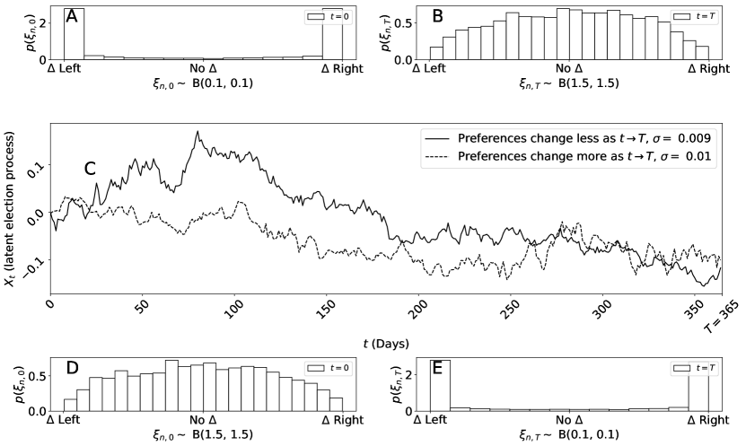
Figure 1: The random walk latent space election model is an accurate approximation to multiple different population candidate preference updates. The latent election process evolves according to $X_{k+1}=X_{k}+\frac{1}{N}\sum_{1\leq n\leq N}\xi_{n,k}$. The random variable $\xi_{n,k}$ is voting agent $n$’s shift toward the left or right. of the political spectrum at time $k$. In the center panel, the solid curve is a draw from the latent election process resulting from the preference updates $\xi_{n,t}\sim B\left(0.1\frac{T-t}{T}+1.5\frac{t}{T},0.1\frac{T-t}{T}+1.5\frac{t}{T}\right)$, where $B(\alpha,\beta)$ is the Beta distribution and we have set $T=365$. As $t\rightarrow T$, the electorate exhibits increasing resistance to change in their political viewpoints. We display the preference shift distributions at $t=0$ in Panel A and at $t=T$ in Panel B. For contrast, the dashed curve is a draw from the latent election process resulting from $\xi_{n,t}\sim B\left(1.5\frac{T-k}{T}+0.1\frac{k}{T},1.5\frac{T-k}{T}+0.1\frac{k}{T}\right)$, which describes an electorate in which agents more often have changing political preferences as $t\rightarrow T$. We show the corresponding preference shift distributions at $t=0$ in Panel D and at $t=T$ in Panel E. Despite these preference updates that are, in some sense, opposites of each other, the latent processes $X_{t}$ are statistically very similar and are both well-modeled by the continuum approximation $\textnormal{d}X_{t}=\sigma\textnormal{d}\mathcal{W}_{t}$.

We display sample realizations of this process for different distributions of $\xi_{n,t_{k}}$ in Fig. 1. Though one distribution of preference changes has a larger variance than the other, the sample paths of $X_{t_{k}}$ are statistically similar for each since $\frac{1}{N}\sum_{n}\xi_{n,t_{k}}$ does not vary much between the distributions. When $N$ is large we can reasonably approximate this discrete agent electoral process by a Wiener process, $\textnormal{d}X_{t}=\sigma\textnormal{d}\mathcal{W}_{t}$, where $\sigma^{2}\approx\text{Var}\left(\frac{1}{N}\sum_{1\leq n\leq N}\xi_{n,t}\right)$, This limit is valid in the limit of large $N$.

If the preference change random variables $\xi_{n,k}$ did not satisfy $E_{n}[\xi_{n,k}]=0$ then the random walk approximation to Eq. 1 would not necessarily be valid. For example, if $\{\xi_{n,k}\}_{k\geq 0}$ were a random walk or were trend-stationary for each $n$, then $\{E_{n}[\xi_{n,k}]\}_{k\geq 0}$ would also respectively be a random walk or trend-stationary. A trend-stationary univariate time series is a stochastic process $x_{t}=f(t)+\varepsilon_{t}$, where $\varepsilon_{t}$ is a stationary process and $f(\cdot)$ is a deterministic function of time nelson1982trends ; dejong1992integration . A univariate time series with a unit root is a time series that can be written as an autoregressive process of order $p$ ($AR(p)$), $x_{t}-\sum_{p^{\prime}=1}^{p}\beta_{p^{\prime}}x_{t-p^{\prime}}=\varepsilon_{t}$, such that the polynomial $z^{p}-\sum_{p^{\prime}=1}^{p}\beta_{p^{\prime}}z^{t-p^{\prime}}=0$ has a root on the unit circle when solved over the complex numbers. A random walk is a special case of the $AR(p)$ process with characteristic polynomial given by $z-1=0$, which has the unit root $z=1$. Trend-stationary and unit-root time series differ fundamentally in that a trend-stationary process subjected to an exogenous shock will eventually revert to its mean function $f(t)$. This is not the case for a stochastic process with a unit root. A unit root or trend-stationary $\xi_{n,k}$ would model a population in which political preferences were undergoing a shift in population mean rather than just in individual preferences.

However, there do exist cases where the random walk approximation is valid even when $E_{n}[\xi_{n,k}]\neq 0$. If the stochastic evolution equation for $E_{n}[\xi_{n,k}]$ has a stationary colored noise with exponentially-decaying covariance function as its solution, then the integral of this noise satisfies a Stratonovich-type equation gardiner1985handbook ; jung1987dynamical ; hanggi1995colored . This equation would be a generalized version of the basic random walk model considered here, but we will not consider this scenario in the remainder of this work.

We denote the control policies of Red and Blue (the functions by which Red and Blue attempt to influence (or prevent influence on) the election) by $u_{\mathrm{R}}(t)$ and $u_{\mathrm{B}}(t)$. These functions are one-dimensional continuous-time stochastic processes (time series). The term “policy” originates from the fields of economics and reinforcement learning bellman1954dynamic ; bellman1966dynamic ; sutton2018reinforcement . These control policies are abstract variables in the context of our model, but we interpret them as expenditures on interference operations. We assume that Red and Blue can affect the mean trajectory of the election but not its volatility (standard deviation of its increments). We make this assumption because $X_{t}$ is an approximation to the process described by Eq. 1. As we show in Fig. 1, the variance of the electoral process does not change much even when the voting population’s underlying preference change distributions have differing variance and kurtosis. Under the influence of Red’s and Blue’s control policies, the election dynamics become

$$\textnormal{d}X_{t}=F(u_{\mathrm{R}}(t),u_{\mathrm{B}}(t))\ \textnormal{d}t+\sigma\ \textnormal{d}\mathcal{W}_{t},\ X_{0}=y.$$ (2)

The function $F$ captures the mechanism by which Red and Blue affect the mean dynamics of the latent electoral process. We assume that $F$ is at least twice continuously-differentiable for connvenience. To first order expansion we have $F(u_{\mathrm{R}}(t),u_{\mathrm{B}}(t))=a_{0}+a_{\mathrm{R}}u_{\mathrm{R}}(t)+a_{\mathrm{B}}u_{\mathrm{B}}(t)+\mathcal{O}(u^{2})$, which is most accurate near $u=0$. We approximate the state equation by

$$\textnormal{d}X_{t}=[u_{\mathrm{R}}(t)+u_{\mathrm{B}}(t)]\ \textnormal{d}t+\sigma\ \textnormal{d}\mathcal{W}_{t},\ X_{0}=y,$$ (3)

since we have assumed zero endogenous drift and can absorb constants into the definition of the control policies. We will use Eq. 3 as the state equation for the remainder of the paper.

II.2 Subgame-perfect Nash equilibria

Red and Blue each seek to minimize separate scalar cost functionals of their own control policy and the other agent’s control policy. We will assume that the agents do not incur a running cost from the value of the state variable, although we will revisit this assumption in Sec. IV. The cost functionals are therefore

$$E_{u_{\mathrm{R}},u_{\mathrm{B}},X}\left\{\Phi_{\mathrm{R}}(X_{T})+\int_{0}^{T}C_{\mathrm{R}}(u_{\mathrm{R}}(t),u_{\mathrm{B}}(t))\ \textnormal{d}t\right\},$$ (4)

and

$$E_{u_{\mathrm{R}},u_{\mathrm{B}},X}\left\{\Phi_{\mathrm{B}}(X_{T})+\int_{0}^{T}C_{\mathrm{B}}(u_{\mathrm{R}}(t),u_{\mathrm{B}}(t))\ \textnormal{d}t\right\}.$$ (5)

The functions $C_{\mathrm{R}}$ and $C_{\mathrm{B}}$ represent the running cost or benefit of conducting election interference operations. We assume the cost functions have the form

$$C_{i}(u_{\mathrm{R}},u_{\mathrm{B}})=u_{i}^{2}-\lambda_{i}u_{\lnot i}^{2}$$ (6)

for $i\in\{\mathrm{R},\mathrm{B}\}$. The notation $\lnot i$ indicates the set of all other players. For example, if $i=\mathrm{R}$, $\lnot i=\mathrm{B}$. This notation originates in the study of noncooperative economic games. The non-negative scalar $\lambda_{i}$ parameterizes the utility gained by player $i$ from observing player $\lnot i$’s effort. If $\lambda_{i}>0$, player $i$ gains utility from player $\lnot i$’s expending resources, while if $\lambda_{i}=0$, player $i$ has no regard for $\lnot i$’s level of effort but only for their own running cost and the final cost. Our assumption that cost accumulates quadratically with magnitude of the control policy is common in optimal control theory kappen2007introduction ; aastrom2012introduction ; georgiou2013separation . We can justify the functional form of Eq. 6 as follows. Suppose that an arbitrary analytic cost function for player $i$ as $\mathcal{C}_{i}(u_{\mathrm{R}},u_{\mathrm{B}})=\mathcal{C}^{(i)}(u_{i})-\lambda_{i}\mathcal{C}^{(\lnot i)}(u_{\lnot i})$. We make the following assumptions:

• It is equally costly to for player $i$ to conduct operations that favor candidate A or candidate B. This imposes the constraint that $\mathcal{C}^{(i)}$ and $\mathcal{C}^{(\lnot i)}$ are even functions.

• Player $i$ conducting no interference operations results in player $i$’s incurring no direct cost from this choice. In other words, if $u_{i}(t)=0$ at some $t$, player $i$ does not incur any cost from this.

With these assumptions, the first non-zero term in the Taylor expansion of $\mathcal{C}_{i}$ is given by Eq. 6.

II.2.1 Choice of final conditions

Finding optimal play in noncooperative games often requires solving the game backward through time zermelo1913anwendung ; nash1951non ; fudenberg1989noncooperative ; mas1995microeconomic . Therefore, we must define final conditions that specify the cost that Red and Blue incur from the actual election result $\phi(X_{T})$. Red and Blue might have different final conditions because of their qualitatively distinct objectives. Since Red wants to influence the outcome of the election in Blue’s country in favor of candidate A, their final cost function $\Phi_{\mathrm{R}}$ must satisfy $\Phi_{\mathrm{R}}(x)<\Phi_{\mathrm{R}}(y)$ for all $x<0$ and $y>0$. In the final conditions that we are about to present, we also assume that $\Phi_{\mathrm{R}}$ is monotonically non-decreasing everywhere. We relax these assumption in Sec. III when we confront this model with election interference-related data. To the extent that this model describes reality, it is probably not true that these restrictive assumptions on the final condition are always satisfied. However, one simple final condition that satisfies these requirements is $\Phi_{\mathrm{R}}(x)=c_{0}+c_{1}x$, but this allows the unrealistic limiting condition of infinite benefit if candidate A gets 100% of the vote in the election and infinite cost if candidate A gets 0% of the vote. We will also consider two Red final conditions with cost that remains bounded as $x\rightarrow\pm\infty$: one smooth, $\Phi_{\mathrm{R}}(x)=\tanh(x)$; and one discontinuous, $\Phi_{\mathrm{R}}(x)=\Theta(x)-\Theta(-x)$. By $\Theta(\cdot)$ we mean the Heaviside step function.

Blue wants to reduce the overall impact of Red’s interference operations on the electoral process. Since Blue is a priori indifferent between the outcomes of the election, it initially seems that $\Phi_{\mathrm{B}}(x)=0$. However, if $\lambda_{\mathrm{B}}=0$, this results in Blue taking no action due to the functional form of Eq. 6. In other words, if Blue does not gain utility from Red expending resources, then Blue will not try to stop Red from interfering in an election in Blue’s country. Hence we believe that Blue cannot be indifferent about the election outcome.

We present three possible final conditions representing Blue’s preferences over the election result. Blue might believe that a result was due to Red’s interference if $X_{T}$ is too far from $E_{0}[X_{T}]=0$. An example of a smooth function that represents this belief is $\Phi_{\mathrm{B}}(x)=\frac{1}{2}x^{2}$. However, this neglects the reality that Red’s objective is not to have either candidate A or candidate B win by a large margin, but rather to have candidate A win, i.e., have $X_{T}<0$. Thus Blue might be unconcerned about larger positive values of the state variable and, modifying the previous function suitably, have $\Phi_{\mathrm{B}}(x)=\frac{1}{2}x^{2}\Theta(-x)$. Alternatively, Blue may accept the result of the election if it does not deviate “too far” from the initial expected value. An example of a discontinuous final condition that represents these preferences is $\Phi_{\mathrm{B}}(x)=\Theta(|x|-\Delta)-\Theta(\Delta-|x|)$, where $\Delta>0$ is Blue’s accepted margin of error.

Though we could propose many other possible final conditions, these example functions demonstrate some possible payoff structures. We include:

• “First-order” functions that could result from the Taylor expansion about zero of an arbitrary analytic final condition. These functions are linear, in the case of Red’s antisymmetric final condition, and quadratic in the case of Blue’s smooth symmetric final condition (which is the first non-constant term in the Taylor expansion of an even analytic function);

• Smooth functions that represent bounded preferences over the result of the electoral process and the recognition that Red favors one candidate in particular; and

• Discontinuous final conditions that model “all-or-nothing” preferences over the outcome (either candidate A wins or they do not; either Red interferes less than a certain amount or they interfere more).

These functions do not capture some behavior that might exist in real election interference operations. For example, Red’s preferences could be as follows: “we would prefer that candidate A wins the election, but if they cannot, then we would like candidate B to win by a landslide so that we can claim the electoral system in Blue’s country was rigged against candidate A”. These preferences correspond to a final condition with a global minimum at some $x<0$ but a secondary local minimum at $x\gg 0$. This situation is not modeled by any of the final conditions that we have stated. In Sec. III we relax the assumption that the final conditions are parameterized according to any of the functional forms considered in thise section and instead infer them from observed election and election interference proxy data using the method described in Sec. II.2.3.

II.2.2 Value functions

Applying the dynamic programming principle bellman1954dynamic ; bellman1966dynamic to Eqs. 3, 4, and 5 leads to a system of coupled Hamilton-Jacobi-Bellman equations for the Red and Blue value functions,

$$-\frac{\partial V_{\mathrm{R}}}{\partial t}=\min_{u_{\mathrm{R}}}\left\{\frac{\partial V_{\mathrm{R}}}{\partial x}[u_{\mathrm{R}}+u_{\mathrm{B}}]+u_{\mathrm{R}}^{2}-\lambda_{\mathrm{R}}u_{\mathrm{B}}^{2}+\frac{\sigma^{2}}{2}\frac{\partial^{2}V_{\mathrm{R}}}{\partial x^{2}}\right\},$$ (7)

and

$$-\frac{\partial V_{\mathrm{B}}}{\partial t}=\min_{u_{\mathrm{B}}}\left\{\frac{\partial V_{\mathrm{B}}}{\partial x}[u_{\mathrm{R}}+u_{\mathrm{B}}]+u_{\mathrm{B}}^{2}-\lambda_{\mathrm{B}}u_{\mathrm{R}}^{2}+\frac{\sigma^{2}}{2}\frac{\partial^{2}V_{\mathrm{B}}}{\partial x^{2}}\right\}.$$ (8)

The dynamic programming principle does not result in an Isaacs equation because the game is not zero-sum and the cost functionals for Red and Blue can have different functional forms. (The Isaacs equation is a nonlinear elliptic or parabolic equation that arises in the study of two-player, zero-sum games in which one player attempts to maximize a functional and the other player attempts to minimize it buckdahn2008stochastic ; pham2014two .) Performing the minimization with respect to the control variables gives the Nash equilibrium control policies,

$$u_{\mathrm{R}}(t) =-\frac{1}{2}\frac{\partial V_{\mathrm{R}}}{\partial x}\bigg{|}_{(t,X_{t})}$$ (9)

$$u_{\mathrm{B}}(t) =-\frac{1}{2}\frac{\partial V_{\mathrm{B}}}{\partial x}\bigg{|}_{(t,X_{t})},$$ (10)

and the exact functional forms of Eqs. 7 and 8,

$$-\frac{\partial V_{\mathrm{R}}}{\partial t} =-\frac{1}{4}\left(\frac{\partial V_{\mathrm{R}}}{\partial x}\right)^{2}-\frac{1}{2}\frac{\partial V_{\mathrm{R}}}{\partial x}\frac{\partial V_{\mathrm{B}}}{\partial x}-\frac{\lambda_{\mathrm{R}}}{4}\left(\frac{\partial V_{\mathrm{B}}}{\partial x}\right)^{2}+\frac{\sigma^{2}}{2}\frac{\partial^{2}V_{\mathrm{R}}}{\partial x^{2}},\qquad V_{\mathrm{R}}(x,T)=\Phi_{\mathrm{R}}(x);$$ (11)

$$-\frac{\partial V_{\mathrm{B}}}{\partial t} =-\frac{1}{4}\left(\frac{\partial V_{\mathrm{B}}}{\partial x}\right)^{2}-\frac{1}{2}\frac{\partial V_{\mathrm{B}}}{\partial x}\frac{\partial V_{\mathrm{R}}}{\partial x}-\frac{\lambda_{\mathrm{B}}}{4}\left(\frac{\partial V_{\mathrm{R}}}{\partial x}\right)^{2}+\frac{\sigma^{2}}{2}\frac{\partial^{2}V_{\mathrm{B}}}{\partial x^{2}},\qquad V_{\mathrm{B}}(x,T)=\Phi_{\mathrm{B}}(x).$$ (12)

When solved over the entirety of state space, solutions to Eqs. 11 and 12 constitute the strategies of a subgame-perfect Nash equilibrium. No matter the action taken by player $\lnot i$ at time $t$, player $i$ is able to respond with the optimal action at time $t+\textnormal{d}t$. This is the (admittedly-informal) definition of a subgame-perfect Nash equilibrium in a continuous-time differential game mas1995microeconomic . Given the solution pair $V_{\mathrm{R}}(x,t)$ and $V_{\mathrm{B}}(x,t)$, we can write the distribution of $x$, $u_{\mathrm{R}}$, and $u_{\mathrm{B}}$ analytically. Substitution of Eqs. 9 and 10 into Eq. 3 gives $\textnormal{d}x=-\frac{1}{2}\left\{\frac{\partial V_{\mathrm{R}}}{\partial x}|_{(t,x)}+\frac{\partial V_{\mathrm{B}}}{\partial x}|_{(t,x)}\ \right\}\textnormal{d}t+\sigma\textnormal{d}\mathcal{W}$. We discretize this equation over $N$ timepoints to obtain

$$x_{n+1}-x_{n}+\frac{\Delta t}{2}\left[V_{\mathrm{R}n}^{\prime}+V_{\mathrm{B}n}^{\prime}\right]$$ (13)

$$\qquad-(\Delta t)^{1/2}\sigma w_{n}-y\delta_{n,0}=0,$$

with $w_{n}\sim\mathcal{N}(0,1)$, $\Delta t=t_{n+1}-t_{n}$, and $n=0,...,N-1$ and where we have put $V^{\prime}_{in}\equiv V_{i}^{\prime}(x_{n},t_{n})$. Thus the distribution of an increment of the latent electoral process is

$$p(x_{n+1}|x_{n})=\frac{1}{\sqrt{2\pi\sigma^{2}\Delta t}}e^{-\frac{\Delta t}{2\sigma^{2}}(\frac{x_{n+1}-x_{n}}{\Delta t}+\frac{1}{2}[V^{\prime}_{\mathrm{R}n}+V^{\prime}_{\mathrm{B}n}]-y\frac{\delta_{n0}}{\Delta t})^{2}}.$$ (14)

Now, using the Markov property of $X_{t}$, we have

$$p(x_{1},...,x_{N}|x_{0}) =\prod_{n=0}^{N-1}p(x_{n+1}|x_{n})$$ (15)

$$=\frac{1}{(2\pi\sigma^{2}\Delta t)^{N/2}}\exp\left\{-\frac{1}{2\sigma^{2}}S(x_{1},...,x_{N})\right\},$$ (16)

where

$$S(x_{1},...,x_{N}) =\sum_{n=0}^{N-1}\Delta t\Big{[}\frac{x_{n+1}-x_{n}}{\Delta t}$$ (17)

$$\quad+\frac{1}{2}[V_{\mathrm{R}n}^{\prime}+V_{\mathrm{B}n}^{\prime}]-\frac{y\delta_{n,0}}{\Delta t}\Big{]}^{2}.$$

Taking $N\rightarrow\infty$ as $N\Delta t=T$ remains constant gives a functional Gaussian distribution,

$$p(x(0\rightarrow T)|x_{0})=\frac{1}{\mathcal{Z}}\exp\left\{-\frac{1}{2\sigma^{2}}S[x(0\rightarrow T)]\right\},$$ (18)

with action

$$S[x(0\rightarrow T)] =\int_{0}^{T}\Big{[}\frac{\textnormal{d}x}{\textnormal{d}t}+\frac{1}{2}\Big{(}\frac{\partial V_{\mathrm{R}}}{\partial x}\Big{|}_{x=x(t)}\frac{\partial V_{\mathrm{B}}}{\partial x}\Big{|}_{x=x(t)}\Big{)}$$ (19)

$$\quad-y\delta(t-t_{0})\Big{]}^{2}\ \textnormal{d}t$$

and partition function

$$\mathcal{Z}=\int_{x(0)}^{x(T)}\mathcal{D}x(0\rightarrow T)\exp\left\{-\frac{1}{2\sigma^{2}}S[x(0\rightarrow T)]\right\}.$$ (20)

We have denoted by $x(s\rightarrow t)$ the actual path followed by the latent state from time $s$ to time $t$. The measure $\mathcal{D}x(0\rightarrow T)$ is classical Wiener measure. Since $u_{\mathrm{R}}(0\rightarrow T)$ and $u_{\mathrm{B}}(0\rightarrow T)$ are deterministic time-dependent functions of $x(0\rightarrow T)$, we can find their distributions explicitly using the probability distribution Eq. 16 and the appropriate time-dependent Jacobian transformation. These analytical results are of limited utility because we are unaware of analytical solutions to the system given in Eqs. 11 and 12, and hence $V_{\mathrm{R}}^{\prime}(x,t)$ and $V_{\mathrm{B}}^{\prime}(x,t)$ must be approximated. In Sec. II.3 we will derive analytical results that are valid when player $i$ announces a credible commitment to a particular control path.

We find the value functions $V_{\mathrm{R}}(x,t)$ and $V_{\mathrm{B}}(x,t)$ numerically through backward iteration, enforcing a Neumann boundary condition at $x=\pm 3$, which corresponds to bounding polling popularity of candidate B from below by $100\times\phi(-3)=4.7\%$ and from above by $100\times\phi(3)=95.3\%$ . We display example realizations of the value functions for different $\lambda_{i}$ and final conditions in Fig. 2.

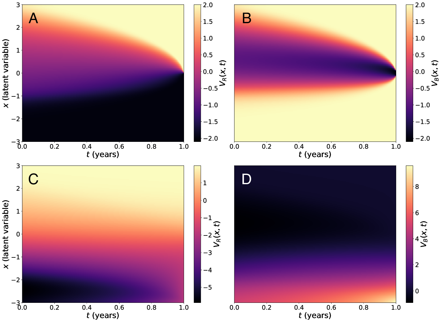
Figure 2: Example value functions corresponding to the system Eqs. 11 and 12. Panels A and B display $V_{\mathrm{R}}(x,t)$ and $V_{\mathrm{B}}(x,t)$ respectively for $\lambda_{\mathrm{R}}=\lambda_{\mathrm{B}}=0$, $\Phi_{\mathrm{R}}(x)=2[\Theta(x)-\Theta(-x)]$, and $\Phi_{\mathrm{B}}(x)=2[\Theta(|x|-0.1)-\Theta(0.1-|x|)]$ with $\Delta=0.1$, while panels C and D display $V_{\mathrm{R}}(x,t)$ and $V_{\mathrm{B}}(x,t)$ respectively for $\lambda_{\mathrm{R}}=\lambda_{\mathrm{B}}=2$, $\Phi_{\mathrm{R}}(x)=2\tanh(x)$, and $\Phi_{\mathrm{B}}(x)=\frac{1}{2}x^{2}\Theta(-x)$. For each solution we enforce Neumann no-flux boundary conditions and set $\sigma=0.6$. The solution is computed on a grid with $x\in[-3,3]$, setting $\textnormal{d}x=0.025$, and integrating for $N_{t}=$ 8,000 timesteps.

The value functions display diffusive dynamics because the state equation is driven by Gaussian white noise. The value functions also depend crucially on the final condition. When the final conditions are discontinuous (as in the top panels of Fig. 2) the derivatives of the value function reach larger magnitudes and vary more rapidly than when the final conditions are continuous. This has consequences for the game-theoretic interpretation of these results, as we discuss in Sec. II.2.4. Fig. 2 also demonstrates that the extrema of the value functions are not as large in magnitude when $\lambda_{\mathrm{R}}=\lambda_{\mathrm{B}}=0$ as when $\lambda_{\mathrm{R}}=\lambda_{\mathrm{B}}=2$; this is because higher values of $\lambda_{i}$ mean that player $i$ derives utility not only from the final outcome of the game but also from causing player $\lnot i$ to expend resources in the game.

Eqs. 7 and 8 give the closed-loop control policies given the current state $X_{t}$ and time $t$, $u_{\mathrm{R}}$ and $u_{\mathrm{B}}$. We display examples of $u_{\mathrm{R}}$, $u_{\mathrm{B}}$ and the electoral process $Z_{t}$ in Fig. 3.

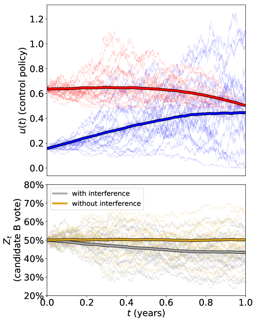
Figure 3: We display realizations of $u_{\mathrm{R}}$ and $u_{\mathrm{B}}$ in the top panel and paths of the electoral process in the bottom panel. We draw these realizations from the game simulated with parameters $\lambda_{\mathrm{R}}=\lambda_{\mathrm{B}}=2$, $\Phi_{\mathrm{R}}(x)=x$, and $\Phi_{\mathrm{B}}(x)=\frac{1}{2}x^{2}\Theta(-x)$. For this parameter set, Blue is fighting a losing battle since optimal play by both players results in lower $E[Z_{t}]$ than for the electoral process without any interference.

For this example, we simulate the game with parameters $\lambda_{\mathrm{R}}=\lambda_{\mathrm{B}}=2$, $\Phi_{\mathrm{R}}(x)=x$, and $\Phi_{\mathrm{B}}(x)=\frac{1}{2}x^{2}\Theta(-x)$. We plot the control policies in the top panel. The mean control policies $E[u_{\mathrm{R}}]$ and $E[u_{\mathrm{B}}]$ are displayed in thicker curves. For this parameter set, it is optimal for Red to begin play with a larger amount of interference than Blue does and on average decrease the level of interference over time. Throughout the game Blue increases their resistance to Red’s interference. Even though Blue resists Red’s interference, Red is able to accomplish their objective of causing candidate A to win.

II.2.3 Inference and prediction

The solutions to Eqs. 11 and 12 are functions of the final conditions $V_{\mathrm{R}}(x,T)=\Phi_{\mathrm{R}}(x)$ and $V_{\mathrm{B}}(x,T)=\Phi_{\mathrm{B}}(x)$. It is possible to perform both inference and prediction at times $t<T$ even when $\Phi_{\mathrm{R}}(x)$ and $\Phi_{\mathrm{B}}(x)$ are not known. To do this, we assume that the system given by Eqs. 11 and 12 has a unique solution given particular final conditions $\Phi_{\mathrm{R}}$ and $\Phi_{\mathrm{B}}$. Though we have numerical evidence to suggest that such solutions do exist and are unique, we have not proved that this is the case. In inference, we want to find the distributions of values of some unobserved parameters of the system. We will suppose that we want to infer $\Phi_{\mathrm{R}}$ and $\Phi_{\mathrm{B}}$ given the observed paths $x(0\rightarrow t),u_{\mathrm{R}}(0\rightarrow t),u_{\mathrm{B}}(0\rightarrow t)$ with $t<T$. For simplicity we assume that we know all other parameters of Eqs. 11 and 12 with certainty. Then the posterior distribution of $\Phi_{\mathrm{R}}$ and $\Phi_{\mathrm{B}}$ reads

$$p(\Phi_{\mathrm{R}},\Phi_{\mathrm{B}}|X_{s})\propto p(x(0\rightarrow t)|\Phi_{\mathrm{R}},\Phi_{\mathrm{B}})\ p(\Phi_{\mathrm{R}},\Phi_{\mathrm{B}}).$$ (21)

The likelihood $p(x(0\rightarrow t)|\Phi_{\mathrm{R}},\Phi_{\mathrm{B}})$ is Gaussian, as shown in Eq. 18, and depends on the time-dependent Jacobian transformtions defined implicitly by the solutions of Eqs. 11 and 12. The prior over final conditions $p(\Phi_{\mathrm{R}},\Phi_{\mathrm{B}})$ can be set proportional to unity if we want to use a maximum-likelihood approach and not account for our prior beliefs about the form of $\Phi_{\mathrm{R}}$ and $\Phi_{\mathrm{B}}$. We can approximate $\Phi_{\mathrm{R}}$ and $\Phi_{\mathrm{B}}$ with functions parameterized by a finite set of parameters $a_{i,k}$, where $i\in\{\mathrm{R},\mathrm{B}\}$ and $k=0,...,K$. The functional prior $p(\Phi_{\mathrm{R}},\Phi_{\mathrm{B}})$ is then approximated by the multivariate distribution $p(k_{\mathrm{R},0},...,k_{\mathrm{R},K},k_{\mathrm{B},0},...,k_{\mathrm{B},K})$. We will take this approach when performing inference in Sec. III.

We can predict future values of $x(t)$, and hence $u_{\mathrm{R}}(t)$ and $u_{\mathrm{B}}(t)$, similarly. Now we want to find the probability of observing $x(t\rightarrow T)$ given observed $x(0\rightarrow t)$. To do this, we integrate out all possible choices of $\Phi_{\mathrm{R}}$ and $\Phi_{\mathrm{B}}$ weighted by their posterior likelihood given the observed path $x(0\rightarrow t)$. The integration is taken with respect to a functional measure, $\mathcal{D}(\Phi_{\mathrm{R}}(x),\Phi_{\mathrm{B}}(x))$. This means that the integration is taken over all possible choices of $\Phi_{\mathrm{R}}$ and $\Phi_{\mathrm{B}}$ that lie in some particular class of functions . As in the case of inference, we can approximate $\Phi_{\mathrm{R}}$ and $\Phi_{\mathrm{B}}$ by functions parameterized by a finite set of parameters $a_{i,k}$ and integrate over the $2K$-dimensional domain of these parameters. In the present work we do not predict any future values of the latent electoral process or control policies.

II.2.4 Dependence of value functions on parameters

We conducted a coarse parameter sweep over $\lambda_{\mathrm{R}}$, $\lambda_{\mathrm{B}}$, $\Phi_{\mathrm{R}}$, and $\Phi_{\mathrm{B}}$ to explore qualitative behavior of this game. We display the results of this parameter sweep for two combinations of final conditions in Figs. 4 and 5. The upper right-hand corner of each panel of the figures displays the final condition of each player. Holding Blue’s final condition of $\Phi_{\mathrm{B}}(x)=\frac{1}{2}x^{2}\Theta(-x)$ constant, we compare the means and standard deviations of the Nash equilibrium strategies $u_{\mathrm{R}}(t)$ and $u_{\mathrm{B}}(t)$ across values of the coupling parameters $\lambda_{\mathrm{R}},\lambda_{\mathrm{B}}\in[0,3]$ as Red’s final condition changes from $\Phi_{\mathrm{R}}(x)=\tanh(x)$ to $\Phi_{\mathrm{R}}(x)=\Theta(x)-\Theta(-x)$.

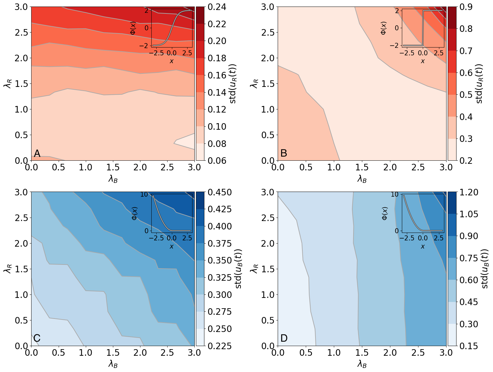
Figure 4: Example sweeps over the coupling parameters $\lambda_{\mathrm{R}}$ and $\lambda_{\mathrm{B}}$ when Blue’s final condition is set to $\Phi_{\mathrm{B}}(x)=\frac{1}{2}x^{2}\Theta(-x)$. We vary the coupling parameters over $[0,3]$ and display the resulting standard deviation of the control policies $u_{\mathrm{R}}(x)$ and $u_{\mathrm{B}}(x)$. Panels A and B represent one coupled system of equations, while panels C and D represent a coupled system of equations with a different set of final conditions. In panel A, Red’s value function is set to $\Phi_{\mathrm{R}}(x)=\tanh(x)$, while in panel B it is given by $\Phi_{\mathrm{R}}(x)=\Theta(x)-\Theta(-x)$, where $\Theta(\cdot)$ is the Heaviside function. We display a glyph of the corresponding final condition in the upper right corner of each panel. Changing Red’s continuous final condition $\tanh(x)$ to the discontinuous $\Theta(x)-\Theta(-x)$ results in substantially increased variation in the control policies of both players.

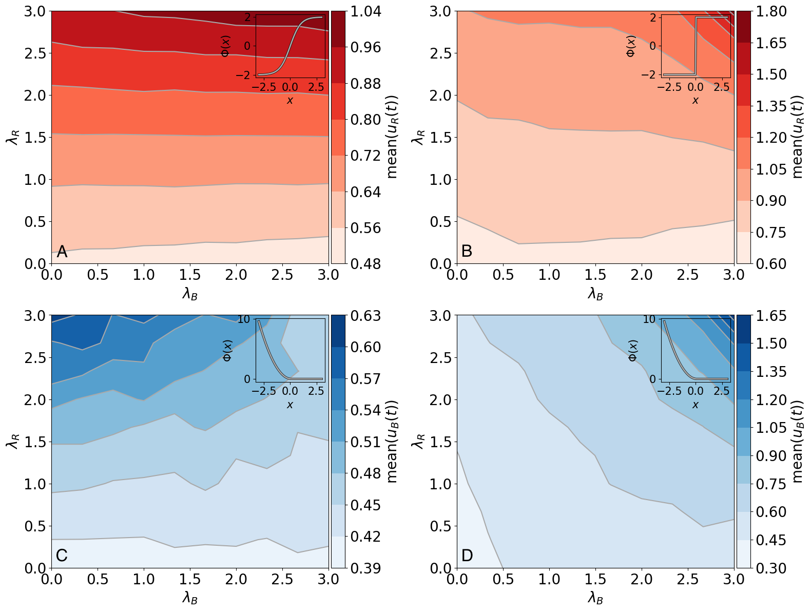
Figure 5: Example sweeps over the coupling parameters $\lambda_{\mathrm{R}}$ and $\lambda_{\mathrm{B}}$ when Blue’s final condition is set to $\Phi_{\mathrm{B}}(x)=\frac{1}{2}x^{2}\Theta(-x)$. We vary the coupling parameters over $[0,3]$ and display the resulting means of the control policies $u_{\mathrm{R}}(x)$ and $u_{\mathrm{B}}(x)$. Panels A and B represent one coupled system of equations, while panels C and D represent a coupled system of equations with a different set of final conditions. In panel A, Red’s value function is set to $\Phi_{\mathrm{R}}(x)=\tanh(x)$, while in panel B it is given by $\Phi_{\mathrm{R}}(x)=\Theta(x)-\Theta(-x)$. Altering Red’s final condition from continuous to discontinuous causes a greater than 100% increase in the maximum value of the mean of Blue’s control policy.

For these combinations of final conditions, higher values of the coupling parameters $\lambda_{i}$ cause the control policies to have higher variance. This increase in variance is more pronounced when Red’s final condition is discontinuous, which is sensible since in this case $\lim_{t\rightarrow T^{-}}u_{\mathrm{R}}(x,t)=-\frac{1}{2}\delta(x)$. Appendix A contains similar figures for each $3^{2}=9$ combinations of Red example final conditions, $\Phi_{\mathrm{R}}(x)\in\left\{\tanh(x),\Theta(x)-\Theta(-x),x\right\}$ and Blue example final conditions, $\Phi_{\mathrm{B}}(x)\in\left\{\frac{1}{x}x^{2},\frac{1}{2}x^{2}\Theta(-x),\Theta(|x|-\Delta)-\Theta(\Delta-|x|)\right\}$. We also find that certain combinations of parameters lead to an “arms-race” effect in both players’ control policies. For these parameter combinations, Nash equilibrium strategies entail superexponential growth in the magnitude of each player’s control policy near the end of the game. Figure 6 displays $E[u_{\mathrm{R}}]$ and $E[u_{\mathrm{B}}]$ for some of these parameter combinations, along with the middle 80% credible interval (10th to 90th percentile) of $u_{\mathrm{R}}(t)$ and $u_{\mathrm{B}}(t)$ for each $t$.

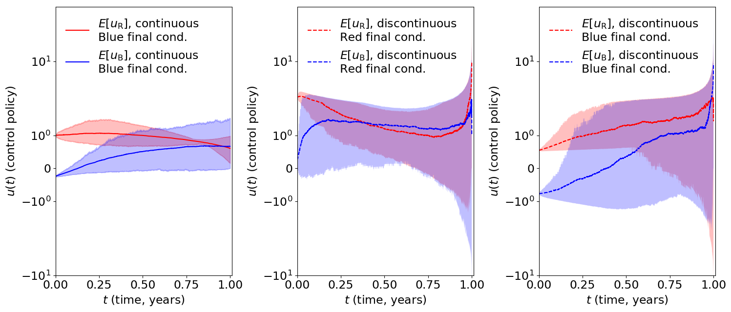
Figure 6: In the case of strong coupling ($\lambda_{\mathrm{R}}$ and $\lambda_{\mathrm{B}}\gg 0$), discontinuous final solutions by either player cause superexponential growth in the magnitude of each player’s control policy. Here we set $\lambda_{\mathrm{R}}=\lambda_{\mathrm{B}}=3$ and integrate three systems, varying only one final condition in each. Panel A displays a system with two continuous final conditions: $\Phi_{\mathrm{R}}(x)=\tanh(x)$ and $\Phi_{\mathrm{B}}(x)=\frac{1}{2}x^{2}\Theta(-x)$. Panel B displays the mean Red and Blue control policies when the Red final condition is changed to $\Phi_{\mathrm{R}}(x)=\Theta(x)-\Theta(-x)$ as the Blue final condition remains equal to $\frac{1}{2}x^{2}\Theta(-x)$, while panel C shows the control policies when $\Phi_{\mathrm{B}}(x)=\Theta(|x|>1)-\Theta(|x|<1)$ and $\Phi_{\mathrm{R}}(x)=\tanh(x)$. The shaded regions correspond to the middle 80 percentiles (10th to 90th percentiles) of $u_{\mathrm{R}}(t)$ and $u_{\mathrm{B}}(t)$ for each $t$. When either player has a discontinuous final condition, the inter-percentile range is substantially wider for both players than when both players have continuous final conditions.

A credible interval for the random variable $Y\sim p(y)$ is an interval into which $Y$ falls with a particular probability chen1999monte . For example, the middle 80% credible interval for $Y\sim p(y)$ is the interval $(a,b)$ for which $\int_{a}^{b}p(y)\ \textnormal{d}y=0.8$ and $\int_{-\infty}^{a}p(y)\ \textnormal{d}y=\int_{b}^{\infty}p(y)\ \textnormal{d}y=0.1$.

This growth in the magnitude of each player’s control policy occurs when either player has a discontinuous final condition. Although a discontinuous final condition by player $i$ leads to a greater increase in mean magnitude of player $i$’s control policy than in player $\lnot i$’s, the standard deviation of each player’s policy exhibits similar superexponential growth. To the extent that this model reflects reality, this points to a general statement about election interference operations: an all-or-nothing mindset by either Red or Blue about the final outcome of the election leads to an arms race that negatively affects both players. This is a general feature of any strategic interaction to which the model described by Eqs. 3 - 5 applies.

II.3 Credible commitment

If player $\lnot i$ credibly commits to playing a particular strategy $v(t)$ on all of $[0,T]$, then the problem of player $i$’s finding a subgame-perfect Nash equilibrium strategy profile becomes an easier problem of optimal control. A credible commitment by player $\lnot i$ to the strategy $v(t)$ means that

• player $\lnot i$ tells player $i$, either directly or indirectly, that player $\lnot i$ will follow $v(t)$; and

• player $i$ should rationally believe that player $\lnot i$ will actually follow $v(t)$.

An example of a mechanism that makes commitment to a strategy credible is the Soviet Union’s “Dead Hand” automated second-strike nuclear response system. This mechanism would launch a full-scale nuclear attack on the United States if it detected a nuclear strike on the Soviet Union yarynich2003c3 ; barrett2016false . The existence of this mechanism made the commitment to the strategy “launch a full-scale nuclear attack on the United States given that any nuclear attack on my country has occurred” credible even though the potential cost to both parties of executing the strategy was high.

When player $\lnot i$ credibly commits to playing $v(t)$, player $i$’s problem reduces to finding the policy $u(t)$ that minimizes the functional

$$E_{u,X}\left\{\Phi(X_{T})+\int_{0}^{T}(u(t)^{2}+\lambda v(t)^{2})\ \textnormal{d}t\right\},$$ (22)

subject to the modified state equation

$$\textnormal{d}x=[u(t)+v(t)]\textnormal{d}t+\sigma\textnormal{d}\mathcal{W}.$$ (23)

Player $i$’s value function is now given by the solution to the HJB equation

$$-\frac{\partial V}{\partial t}=\min_{u}\left\{\frac{\partial V}{\partial x}[u+v]+u^{2}-\lambda v^{2}+\frac{\sigma^{2}}{2}\frac{\partial^{2}V}{\partial x^{2}}\right\}.$$ (24)

Performing the minimization gives the control policy $u(t)=-\frac{1}{2}\frac{\partial V}{\partial x}\Big{|}_{x=x(t)}$ and the explicit functional form of the HJB equation,

$$-\frac{\partial V}{\partial t} =-\frac{1}{4}\left(\frac{\partial V}{\partial x}\right)^{2}+v(t)\frac{\partial V}{\partial x}+\lambda v(t)^{2}+\frac{\sigma^{2}}{2}\frac{\partial^{2}V}{\partial x^{2}},$$ (25)

$$V(x,T) =\Phi(x).$$

II.3.1 Path integral control

Though nonlinear, this HJB equation can be transformed into a backward Kolmogorov equation (BKE) through a change of variables. The BKE can be solved using path integral methods kappen2005path . Setting $V(x,t)=-\eta\log\varphi(x,t)$, substituting in Eq. 25, and performing the differentiation, we are able to remove the nonlinearity if and only if $\frac{\eta^{2}}{4}\frac{1}{\varphi^{2}}\left(\frac{\partial\varphi}{\partial x}\right)^{2}=\frac{\sigma^{2}\eta}{2}\frac{1}{\varphi^{2}}\left(\frac{\partial\varphi}{\partial x}\right)^{2}$. Setting $\eta=2\sigma^{2}$ satisfies this condition. Performing the change of variables, Eq. 25 is now linear and has a time-dependent drift and sink term,

$$\frac{\partial\varphi}{\partial t} =\frac{\lambda}{2\sigma^{2}}v(t)^{2}\varphi(x,t)-v(t)\frac{\partial\varphi}{\partial x}-\frac{\sigma^{2}}{2}\frac{\partial^{2}\varphi}{\partial x},$$ (26)

$$\varphi(x,T) =\exp\left\{-\frac{1}{2\sigma^{2}}\Phi(x)\right\}.$$

Application of the Feynman-Kac formula gives the solution to Eq. 26 as kac1949distributions

$$\varphi(x,t) =\exp\left\{-\frac{\lambda}{2\sigma^{2}}\int_{t}^{T}v(t^{\prime})^{2}\ \textnormal{d}t^{\prime}\right\}\times$$ (27)

$$\quad E_{Y_{t}}\left\{\exp\left[-\frac{1}{2\sigma^{2}}\Phi(Y_{T})\right]\bigg{|}Y_{t}=x\right\},$$

where $Y_{t}$ is defined by

$$\textnormal{d}Y_{t}=v(t)\ \textnormal{d}t+\sigma\textnormal{d}\mathcal{W}_{t},\ Y_{0}=x.$$ (28)

Using this formalism, we apply path integral control to estimate the value function for arbitrary $v(t)$. Fig.  7 displays example path integral solutions to Eq. 25 when player $\lnot i$ credibly commits to playing $v(t)=t^{2}$ for the duration of the game and player $i$’s final cost function takes the form $\Phi(x)=\Theta(|x|-1)-\Theta(1-|x|)$.

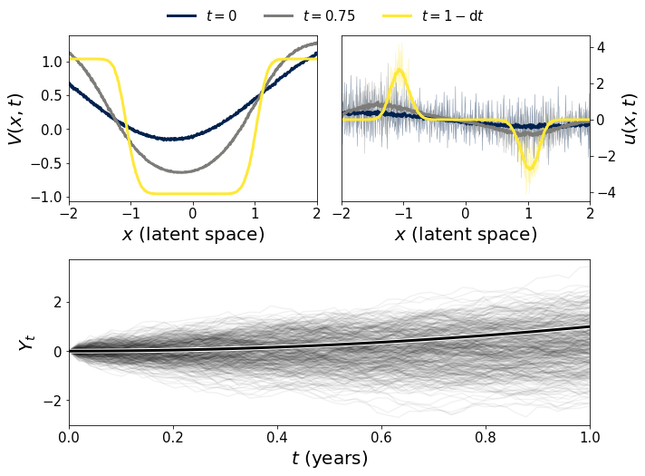
Figure 7: Result of the path integral Monte Carlo solution method applied to Eq. 25 with the final condition $\Phi(x)=\Theta(|x|>1)-\Theta(|x|\leq 1)$ and $v(t)=t^{2}$. Approximate value functions are computed using $N=10000$ trajectories sampled from Eq. 28 for each point $(x,t)$. We display approximate value functions in Panel A for $t\in\{0,0.75,1-\textnormal{d}t\}$ and the corresponding approximate control policies $u(x,t)$ in Panel B, along with smoothed versions of $u(x,t)$, which we denote by $u_{s}(x,t)$, plotted in dashed curves. Panel C displays realizations of $Y_{t}$, the process generating the measure under which the solution is calculated. The analytical control policy at $t=T$ is given by $u(t)=-\frac{1}{2}[\delta(x-1)-\delta(x+1)]$.

In this figure we display the approximate value functions $V(x,t)$ along with their corresponding approximate control policies $u(x,t)=-\frac{1}{2}\frac{\partial V(x,t)}{\partial x}$. We calculated these approximations on a grid of $N_{x}=500$ linearly spaced $x_{n}\in[-2,2]$. Since the approximated $u(x_{n},t)$ are noisy stochastic functions we also plot smoothed versions of them in Fig. 7. These smoothed versions are defined by

$$u_{s}(x_{n},t)=\sum_{n^{\prime}=-k}^{k}u(x_{n+n^{\prime}},t).$$ (29)

We set $k=7$ and hence $u_{s}(x_{n},t)$ are $2k+1=15$-step moving averages of the more noisy $u(x_{n},t)$. As $t\rightarrow T$, $u_{s}(x_{n},t)$ approaches the analytical solution of the control problem at $t=T$, which is given by $u(x,T)=-\frac{1}{2}[\delta(x-1)-\delta(x+1)]$.

In the further restricted case where there is a credible commitment by one party to play a constant control policy $v(t)=v$, we can derive further analytical results. Under this assumption, the probability law corresponding with Eq. 28 is given by

$$u(y,t)=\frac{1}{\sqrt{2\pi\sigma^{2}t}}\exp\left\{\frac{1}{2\sigma^{2}t}[(y-x)-vt]^{2}\right\},$$ (30)

so that the (exponentially-transformed) value function reads

$$\varphi(x,t)=E_{u(y,T-t)}\left[\exp\left\{-\frac{\lambda v^{2}}{2\sigma^{2}}(T-t)\Phi(Y_{T})\right\}\right]$$ (31)

$$\quad=\frac{\exp\left\{-\frac{\lambda v^{2}}{2\sigma^{2}}(T-t)\right\}}{\sqrt{2\pi\sigma^{2}(T-t)}}\times$$ (32)

$$\int\displaylimits_{-\infty}^{\infty}\exp\left\{-\frac{1}{2\sigma^{2}}\left[\Phi(y)+\frac{((y-x)-v(T-t))^{2}}{T-t}\right]\right\}\textnormal{d}y.$$

This integral can be evaluated exactly for many $\Phi(y)$ and, for many other final conditions, it can be approximated using the method of Laplace. When $t\rightarrow T$ so that the denominator of the argument of the exponential in Eq. 31 approaches zero, Laplace’s approximation to the integral reads

$$\int\displaylimits_{-\infty}^{\infty}\exp\left\{-\frac{1}{2\sigma^{2}}\left[\Phi(y)+\frac{((y-x)-v(T-t))^{2}}{T-t}\right]\right\}\textnormal{d}y$$ (33)

$$\quad\approx\sqrt{2\pi\sigma^{2}(T-t)}\exp\left\{-\frac{1}{2\sigma^{2}}\Phi(x+(T-t)v)\right\}.$$

Inverting the transformation $\varphi$, the value function is approximated by

$$V(x,t)=\lambda v^{2}(T-t)+\Phi(x+(T-t)v),$$ (34)

and the control policy by

$$u(x,t)=-\frac{1}{2}\Phi^{\prime}(x+(T-t)v).$$ (35)

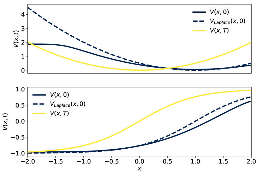
Figure 8: When player $\lnot i$ commits to playing a constant strategy profile $v(t)=v$ for a fixed interval of time, an analytic approximate form for player $i$’s value function $V(x,t)$ is given by $V(x,t)\approx\lambda v^{2}(T-t)+\Phi(x+(T-t)v)$. We show the numerically-determined value functions at time $t=0$ in solid black curves, We display the Laplace approximations at $t=0$ in dashed black curves. The lighter-hue curves are the value functions at the final time $T$, i.e., the respective final conditions. The top panel demonstrates results for the final condition $\Phi(x)=\frac{1}{2}x^{2}$, while the bottom panel has $\Phi(x)=\tanh(x)$.

We display the results of approximating the value function with Eq. 34 at $t=0$ in Fig.  8, along with the actual numerically-determined value function at both $t=0$ and, for reference, $t=T$.

II.3.2 Dependence on a free parameter

The Laplace-approximated value function may depend on a free parameter $a$ that can be used as a “control knob” to adjust the approximation. For example, player $i$ might use $a$ to tune the sensitivity of the approximation to the electoral process’s distance from a dead-heat. Ideally, the approximated control policy should have similar scaling and asymptotic properties as the true control policy. Solving an optimization problem for optimal values of $a$ is be one approach to satisfying this desideratum.

As a case study we consider the behavior of the Laplace-approximated value function $V^{(a)}(x,t)$ and its corresponding control policy $u^{(a)}(x,t)$ when we set $\Phi^{(a)}(x)=\tanh(ax)$. We consider this specific example because $\Phi^{(a)}(x)\rightarrow\Theta(x)-\Theta(-x)$ as $a\rightarrow+\infty$. This limit can be the source of complicated behavior in a variety of fields such as piecewise-smooth dynamical systems (both deterministic and stochastic) chen2013weak ; leifeld2015persistence , Coulombic friction kanazawa2015asymptotic , and evolutionary biology piltz2018inferring .

Fig. 9 displays player $i$’s exponentially-transformed value function Eq. 31 with final condition $\Phi_{i}(x)=\tanh(ax)$. Here player $\lnot i$ credibly commits to playing a constant strategy of $v=0.01$. As $t\rightarrow T$, larger values of $a$ lead to a sharp boundary betweeen regions of the state space that are costly for player $i$ (positive values of $x$) and those that are less costly (negative values of $x$). This behavior is qualitatively similar to behavior arising from the final condition $\Phi_{i}(x)=\Theta(x)-\Theta(-x)$. However, we will show that that there are significant scaling differences in the control policies resulting from using $\Phi(x)$ versus $\Phi^{(a)}(x)$.

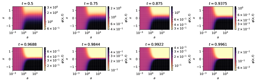
Figure 9: If player $\lnot i$ credibly commits to a strategy of playing a constant strategy with value equal to $v$ for the entire duration of the game, player $i$’s (exponentially-transformed) value function $\varphi(x,t)$ has an integral representation given by Eq. 31. We display dynamics of $\varphi(x,t)$ with the final condition set to $\Phi(x)=\tanh(ax)$. We calculated this value function for $x\in\left(-\frac{3}{2},\frac{3}{2}\right)$ and logarithmically equally-spaced values of $a\in[10^{-3},10^{5}]$. For $a<10^{-1}$, the value function is nearly constant. When $a>10^{1}$, $\frac{\partial}{\partial x}\varphi(x,t)$ increases in magnitude near $x=0$ as $t\rightarrow T$.

From Eqs. 33 and 34, we approximate the value function by

$$V^{(a)}(x,t)\approx\lambda v^{2}(T-t)+\tanh\left\{a[x+v(T-t)]\right\},$$ (36)

and hence the control policy is approximately

$$u^{(a)}(x,t)\approx-\frac{a}{2}\mathrm{sech}^{2}\left\{a[x+v(T-t)]\right\},$$ (37)

with both expansions increasingly accurate as $t\rightarrow T$. When $\Phi(x)=\Theta(x)-\Theta(-x)$, we can compute the value function analytically:

$$\frac{1}{\sqrt{2\sigma^{2}(T-t)}}\int\displaylimits_{-\infty}^{\infty}\exp\left\{-\frac{1}{2\sigma^{2}}\left[\Theta(y)-\Theta(-y)+\frac{((y-x)-v(T-t))^{2}}{T-t}\right]\right\}\textnormal{d}y$$ (38)

$$\qquad=\cosh\left(\frac{1}{2\sigma^{2}}\right)+\sinh\left(\frac{1}{2\sigma^{2}}\right)\mathrm{erf}\left(-\frac{x+v(T-t)}{\sqrt{2\sigma^{2}(T-t)}}\right),$$

whereupon we find that

$$V(x,t)=\lambda v^{2}(T-t)-2\sigma^{2}\log\left[\cosh\left(\frac{1}{2\sigma^{2}}\right)+\sinh\left(\frac{1}{2\sigma^{2}}\right)\mathrm{erf}\left(-\frac{x+v(T-t)}{\sqrt{2\sigma^{2}(T-t)}}\right)\right]$$ (39)

and

$$u(x,t)=-\sqrt{\frac{2\sigma^{2}}{\pi(T-t)}}\frac{\exp\left(\frac{-(x+v(T-t))^{2}}{2\sigma^{2}(T-t)}\right)}{\coth\left(\frac{1}{2\sigma^{2}}\right)+\mathrm{erf}\left(-\frac{x+v(T-t)}{\sqrt{2\sigma^{2}(T-t)}}\right)}.$$ (40)

The approximate control policy $u^{(a)}(x,t)$ and the limiting control policy have similar negative “bell-like” shapes but also differ in important ways. The true control policy decays as a Gaussian modulated by the asymmetric function $\mathrm{erf}(\cdot)$. The approximate policy decays logistically and hence more slowly than the true control policy. While the approximate policy is symmetric, the true policy is asymmetric due to the error function term. Using the Laplace approximation results in more control being applied to the electoral process than is optimal. This is because the tails of $u^{(a)}(x,t)$ are heavier than those of $u(x,t)$.

We can maximize the similarity between $u^{(a)}(x,t)$ and $u(x,t)$ by letting the free parameter $a$ be a function of $t$ and solving the functional minimization problem

$$\min_{a(t)}\int\displaylimits_{t}^{T}\int\displaylimits_{-\infty}^{\infty}[u^{(a(t))}(x,t)-u(x,t)]^{2}\ \textnormal{d}x\ \textnormal{d}t.$$ (41)

A stationary point of this problem is given by an $a(t)$ that solves

$$\int\displaylimits_{-\infty}^{\infty}[u^{(a(t))}(x,t)-u(x,t)]\frac{\partial u^{(a(t))}(x,t)}{\partial a(t)}\ \textnormal{d}x=0.$$ (42)

We are unable to compute this integral analytically upon substituting Eqs. 37 and 40. We find the solution to this problem by numerically solving Eq. 42 using the secant method for each of 100 linearly-spaced $t\in\left[0.5,0.9975\right]$. We display the optimal $a(t)$, along with the corresponding $u^{(a(t))}(x,t)$ and true $u(x,t)$ in Fig. 10.

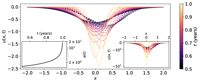
Figure 10: The solution to Eq. 41 is a superexponentially-increasing $a(t)$ parameter in the Laplace method-derived value function $V^{(a)}(x,t)=\tanh(ax)$. We use this value function as an approximation to the exact value function given in Eq. 39. Dashed curves indicate $u(x,t)$, while solid curves indicate $u^{(a)}(x,t)$. The lower-right inset axis displays the same data as the main axis and also includes $u(x,t)$ and $u^{(a)}(x,t)$ at the last simulation timestep, $t=0.9975$, to demonstrate the increasing accuracy of the approximation as $t\rightarrow T$. The lower-left inset displays the optimal $a(t)$.

We find that the optimal $a(t)$ grows superexponentially as $t\rightarrow T$ and that the accuracy of the approximation increases in this limit. This is expected given that $u^{(a)}(x,t)$ is derived using the Laplace approximation and it is in this limit that the Laplace approximation is valid.

Even with the assumption of credible committment to a constant control policy $v$, we can use this theory to approximate the value function in a noncooperative scenario. For arbitrary $v(t)$, expansion about $t+\Delta t$ gives $v(t+\Delta t)=v(t)+v^{\prime}(t)\Delta t,$ leading to an approximate value function iteration over a small time increment $\Delta t$,

$$V(x,t+\Delta t)\approx\lambda v(t)^{2}(T-t)+\Phi(x+(T-t)[v(t)+v^{\prime}(t)\Delta t]).$$ (43)

In application, both of $v(t)$ and $v^{\prime}(t)$ can be estimated from possibly-noisy data on $t^{\prime}\in[0,t]$.

III Application

An example of election interference operations is the Russian military foreign intelligence service (Red team) activity in the 2016 U.S. presidential election contest. Red team attempted to harm one candidate’s (Hilary Clinton’s) chances of winning and aid another candidate (Donald Trump) nyt2019 . Though Russian foreign intelligence had conducted election interference operations in the past at least once before, in the Ukrainian elections of 2014 tanchak2017invisible , the 2015 and 2016 operations were notable in that Red team operatives used the microblogging website Twitter in an attempt to influence the election outcome. When this attack vector was discovered, Twitter shut down accounts associated with Red team activity and all data associated with those accounts was collected and analyzed boatwright2018troll ; badawy2018analyzing ; boyd2018characterizing . There has been analysis of the qualitative and statistical effects of these and other election attack vectors (e.g., Facebook advertisement purchases) on election polling and the outcome of the election ruck2019internet and on the detection of election influence campaigns more generally mesnards2018detecting ; im2019still . However, to the best of our knowledge, there exists no publicly-available effort to reverse-engineer the quantitative nature of the control policies used by Russian military intelligence and by U.S. domestic and foreign intelligence agencies.

We first fit a discrete-time formulation of the model described in Sec. II.1. We then compare it to theoretical predictions by finding values of free parameters in the theoretical model that best describe the observed data and inferred latent controls. We are faced with two distinct sources of uncertainty in this procedure. First, we cannot observe either Red’s or Blue’s control policy directly because foreign and domestic intelligence agencies shroud their activities in secrecy. Second, each player’s final time payoff structure is also secret and unknown to us. To partially circumvent these issues, we construct a two-stage model. The first stage is a Bayesian structural time series model, depicted graphically in Fig. 11, through which we are able to infer distributions of discretized analogues of $u_{\mathrm{R}}(t)$, $u_{\mathrm{B}}(t)$, and $x(t)$. Once we have inferred these distributions, we minimize a loss function that compares the means of these distributions to the means of distributions produced by the model described in Sec. II.1.

We make the simplifying assumptions about the format of the election that we stated in Sec. I when constructing the discrete-time election model. Namely, we assume that only two candidates contest the election and that the election process is modeled by a simple “candidate A versus candidate B” poll. Though there are methods for forecasting elections that make fewer and less restrictive assumptions than these, such as compartmental infection models volkening2018forecasting , prediction markets rothschild2009forecasting , and more sophisticated Bayesian models linzer2013dynamic ; wang2015forecasting , we construct our statistical model to mimic the underlying election model of Sec. II.1. We do this to test the ability of this underlying theoretical model to reproduce inferred control and observed election dynamics.

We can observe neither the Red $u_{\mathrm{R}}(t)$ nor Blue $u_{\mathrm{B}}(t)$ control policies. However, we are able to observe a proxy for $u_{\mathrm{R}}$: the number of tweets sent by Russian military intelligence-associated accounts in the year leading up to the 2016 election . This dataset contains a total of 2,973,371 tweets from 2,848 unique Twitter handles. Of these tweets, a total of 1,107,361 occurred in the year immediately preceding the election (08/11/2015 - 08/11/2016). We grouped these tweets by day and used the time series of total number of tweets on each day as an observable from which we could infer $u_{\mathrm{R}}$. We restricted the time range of the model to begin at the later of the end dates of the Republican National Convention (21 July 2016) and Democratic National Convention (28 July 2016). We did this because the later of these dates, 28 July 2016, is the day on which the race was officially between two major party candidates. Of all Russian military intelligence-associated tweets in 2016, 363,131 occurred during the 102 days beginning on 28 July 2016 and ending the day before Election Day. Though the presence of minor party candidates probably played a role in the result of the election, even the most prominent minor parties (Libertarian and Green) received only single-digit support skibba2016pollsters ; neville2017constrained . We do not model these minor parties and instead consider only the electoral contest between the two major party candidates. We used the RealClearPolitics poll aggregation as a proxy for the electoral process itself , averaging polls that were recorded on the same date and using the earliest date in the date range of the poll if it was conducted over multiple days as the timestamp of that observation. We weighted all polls equally when averaging.

Using these two observed random variables, we fit a Bayesian structural time series model barber2011bayesian of the form presented in Fig. 11.

Figure 11: We approximate the time series components of the analytical model defined in Sec. II.1 by a Bayesian structural time series (BSTS) model. We subsequently confront the BSTS model with 2016 U.S. presidential election data. Observed random variables are denoted by gray-shaded nodes, while latent random variables are represented by unshaded nodes or red ($u_{\mathrm{R},t}$) and blue ($u_{\mathrm{B},t}$) nodes. We observe a noisy election poll, denoted by $Z_{t}$, and a time series of tweets associated with Russian military intelligence, denoted by Tweets. Our objective in this modeling stage is to infer the latent electoral process, denoted by $X_{t}$, and the latent control policies.

We now describe the structure of the model and explain our choices of priors and likelihood functions. In the analytical model, we model the latent control policies $u_{\mathrm{R}}(t)$ and $u_{\mathrm{B}}(t)$ by time- and state-dependent Wiener processes. To see this, recall that the state equation evolves according to a Wiener process and apply Ito’s lemma to the deterministic functions of a random variable $-\frac{1}{2}\frac{\partial V_{\mathrm{R}}}{\partial x^{\prime}}\big{|}_{x^{\prime}=x_{t}}$ and $-\frac{1}{2}\frac{\partial V_{\mathrm{B}}}{\partial x^{\prime}}\big{|}_{x^{\prime}=x_{t}}$, which define the control policies. A discretized version of the Wiener process is a simple Gaussian random walk. We thus model the latent Red and Blue control policies by Gaussian random walks:

$$p(u_{R,t}|u_{R,t-1},\mu_{R},\sigma) =\mathcal{N}(u_{R,t-1}+\mu_{R},\sigma^{2})$$ (44)

$$p(u_{B,t}|u_{B,t-1},\mu_{B},\sigma) =\mathcal{N}(u_{B,t-1}+\mu_{B},\sigma^{2})$$ (45)

Similarly, we model the latent election process by a discretized version of the state evolution equation Eq. 3:

$$p(X_{t}|X_{t-1},u_{R},u_{B})$$ (46)

$$\quad=\mathcal{N}(X_{t-1}+u_{B,t-1}-u_{R,t-1},1)$$

We assume that the latent election model is subject to normal observation error in latent space. Since we chose a logistic function as the link between the latent and real (on $(0,1)$) election spaces, the likelihood for the observed election process is thus given by a Logit-Normal distribution. The pdf of this distribution is

$$p(Z_{t}|X_{t},\sigma_{Z})=\sqrt{\frac{1}{2\pi\sigma_{Z}^{2}}}\frac{\exp\left\{-\frac{(\mathrm{logit}(Z_{t})-X_{t})^{2}}{2\sigma_{Z}^{2}}\right\}}{Z_{t}(1-Z_{t})}.$$ (47)

Though the number of Russian military intelligence tweets that occur on any given day is obviously a non-negative integer, we chose not to model it this way. A common and simple model for a “count” random variable, such as the tweet time series, is a Poisson distribution with possibly-time-dependent rate parameter erlang1909sandsynlighedsregning ; rasch1963poisson ; cox1972regression ; cox1980point . This model imposes a strong assumption on the variance of the count distribution (namely, that the variance and mean are equal) which does not seem realistic in the context of the tweet data. Instead of searching for a discrete count distribution that meets some optimality criterion, we instead normalized the tweet time series to have zero mean and unit variance, making it a continuous random variable rather than a discrete one. We then shifted the time series so that the the new time series was equal to zero on the day during our study with the fewest tweets. We then modeled this time series $\text{Tweets}_{t}$ by a normal observation likelihood,

$$p(\text{Tweets}_{t}|u_{R,t},\sigma_{\text{Tweets}})=\mathcal{N}(u_{R,t},\sigma_{\text{Tweets}}^{2}).$$ (48)

We placed a weakly-informative prior, a Log-Normal distribution, on each standard deviation random variable ($\sigma$, $\sigma_{Z}$, $\sigma_{\text{Tweets}}$), and zero-centered Normal priors on each mean random variable ($\mu_{R},\mu_{B}$). This model is high-dimensional, since the latent time series $X$, $u_{\mathrm{R}}$, and $u_{\mathrm{B}}$ are inferred as $T$-dimensional vectors. In total this model has $3T+5=311$ degrees of freedom.

We display a graphical representation of this model in Fig. 11. We fit this model using the No-U-Turn Sampler algorithm hoffman2014no , sampling 2000 draws from the model’s posterior distribution from each of two independent Markov chains, We do not include 1000 draws per chain of burn-in in the samples from the posterior. The sampler appeared to converge well based on graphical consideration (i.e., the “eye test”) of draws from the posterior predictive distribution of $Z_{t}$ and $\text{Tweets}_{t}$, and, more importantly, because maximum values of Gelman-Rubin statistics gelman1992inference for all variables satisfied $R_{\max}<1.01$ except for that of $\sigma_{Z}$, which had $R_{\max}=1.07646$. Each of these values is well below the level $R=1.1$ advocated by Brooks and Gelman brooks1998general . Fig.  12 displays draws from the posterior and posterior predictive distribution of this model. Panel A displays draws of $X_{t}$ from the posterior distribution, along with $E[X_{t}]$ and $\mathrm{logit}(Z_{t})$, while in panel B we show posterior draws of $u_{\mathrm{R}}$ and $u_{\mathrm{B}}$, along with $E[u_{\mathrm{R}}]$ and $E[u_{\mathrm{B}}]$ in thick red and blue curves respectively. In panel C, we display $\text{Tweets}_{t}$ and draws from its posterior predictive distribution. On 10/06/2016, $\text{Tweets}_{t}$ exhibited a large spike that is very unlikely under the posterior predictive distribution. This spike likely corresponds with a statement made by the U.S. federal government on this date that officially recognized the Russian government as culpable for hacking the Democratic National Committee computers.

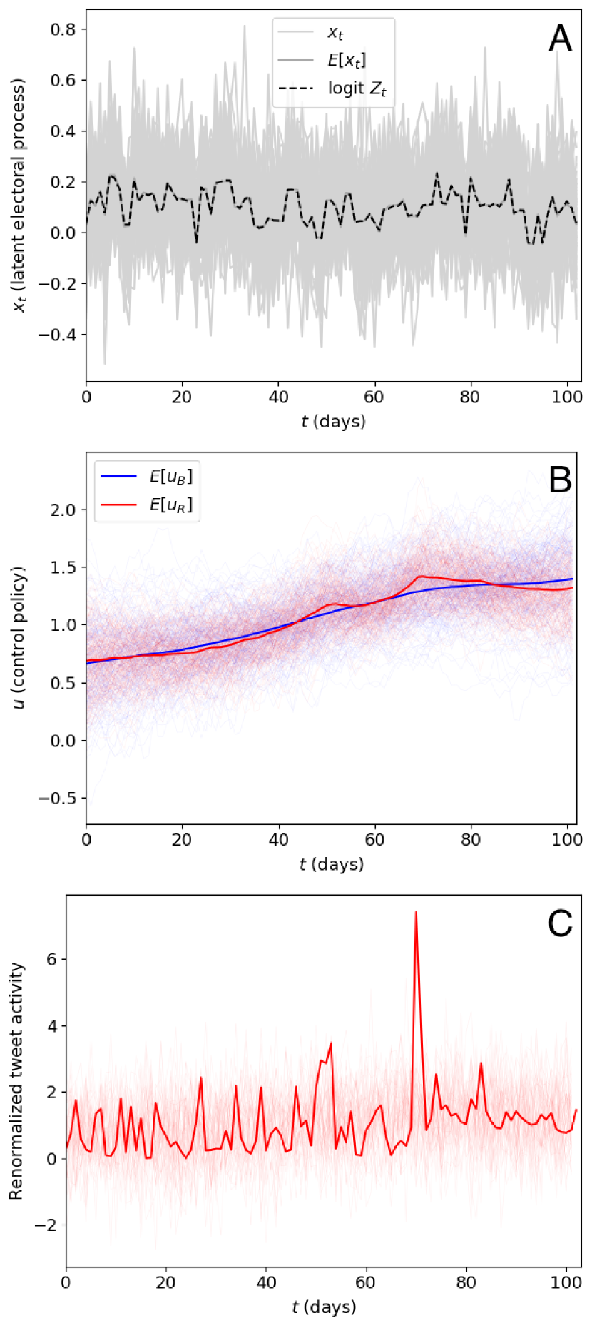
Figure 12: Panel A displays the logit of the observed election time series (black curve) $\mathrm{logit}(Z_{t})$, along with the posterior distribution of the latent electoral process $X_{t}$. Panel B displays the mean latent control policies in thick red and blue curves, along with their posterior distributions. Panel C shows the true tweet time series (subject to the normalization described in the main body) along with draws from its posterior predictive distribution. The large spike in the tweet time series that is very unlikely under the posterior predictive distribution corresponds to the day (10/06/2016) on which the U.S. federal government officially accused Russia of hacking the Democratic National Committee computers.

After inferring the latent control policies and electoral process, we searched for the parameter values $\theta=(\lambda_{\mathrm{R}},\lambda_{\mathrm{B}},\sigma,\Phi_{\mathrm{R}},\Phi_{\mathrm{B}})$ of the theoretical model that best explain the observed data and inferred latent variables. For clarity in reference, we will refer to the theoretical model as $\mathcal{Q}$ and the Bayesian structural time series model as $\mathcal{M}$. We use Legendre polynomials to approximate the final conditions $\Phi_{\mathrm{R}}$ and $\Phi_{\mathrm{B}}$, as discussed in Sec. II.2.3. Setting $\Phi_{i}(x)\approx\sum_{k=0}^{K}a_{ik}P_{k}(x)$, $\mathcal{Q}$’s parameter vector is $\theta=(\lambda_{\mathrm{R}},\lambda_{\mathrm{B}},\sigma,a_{0,r},...,a_{K,r},a_{0,b},...,a_{K,b})$. In contrast with $\mathcal{M}$, $\mathcal{Q}$ has relatively few degrees of freedom since the assumption of state and policy co-evolution via solution of coupled partial differential equations substantially restricts the system’s dynamics. In total, $\mathcal{Q}$ has $2K+3$ free parameters. The smaller the value of $K$, the less accurate the approximation to the true final conditions will be. Conversely, large $K$ could lead to overparameterization of the model and increases the size of the search space. We thus chose $K=10$ as a compromise betweeen these two extremes. With $K=10$, the model has $2K+3=23$ degrees of freedom.

The theoretical model $\mathcal{Q}$ can be viewed as a generative probabilitistic function. To find optimal parameter values, we generate $(\hat{u}_{\mathrm{R}},\hat{u}_{\mathrm{B}},\hat{X})$ from $\mathcal{Q}$ and minimize a loss function of these generated values and the values inferred by $\mathcal{M}$. We defined this loss function as

$$L(\theta|\mathcal{Q}) =\sum_{(y,\hat{y})}\left[\left\lVert\mu_{y}-\mu_{\hat{y}}\right\rVert_{2}^{2}+\eta\sigma_{\hat{y}}\right],$$ (49)

where $y\in\{u_{\mathrm{R}},u_{\mathrm{B}},X\}$ and $\hat{y}\in\{\hat{u}_{\mathrm{R}},\hat{u}_{\mathrm{B}},\hat{X}\}$. We have defined the mean and standard deviation under the corresponding distribution by $\mu$ and $\sigma$ respectively. The $\ell_{2}$ terms in Eq. 49 penalize deviation by $\mathcal{Q}$ from the mean of $\mathcal{M}$’s inferred posterior distribution. The standard deviation term in Eq. 49 imposes a penalty on dispersion. We minimized $L(\theta|\mathcal{Q})$ using a Gaussian-process Bayesian optimization algorithm. The details of this algorithm are beyond the scope of this work but are readily found in any review paper on the subject brochu2010tutorial ; shahriari2015taking ; frazier2018tutorial . Fig. 13 displays the result of this optimization procedure for $K=10$ and $\eta=0.002$.

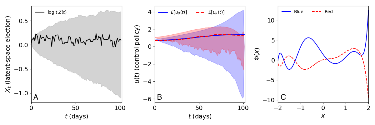
Figure 13: We display credible intervals of latent election process $X$ and Red and Blue control policies, $u_{\mathrm{R}}$ and $u_{\mathrm{B}}$ generated using optimal $\theta=(\lambda_{\mathrm{R}},\lambda_{\mathrm{B}},\sigma,a_{0,r},...,a_{K,r},a_{0,b},...,a_{K,b})$ values. We ran the optimization algorithm with the number of terms of the Legendre expansion of $\Phi_{\mathrm{R}}$ and $\Phi_{\mathrm{B}}$ set to $K=10$ and set the variance regularization in the algorithm to $\eta=0.002$. This resulted in fit parameters of $\lambda_{\mathrm{R}}=0.849$, $\lambda_{\mathrm{B}}=0.727$, and $\sigma=1.509$. Panel A displays draws from the latent electoral process under $\mathcal{Q}$, along with $\mathrm{logit}(Z_{t})$, the logit-transformed real polling popularity process. Panel B displays draws from the distributions of $\hat{u}_{\mathrm{R}}$ and $\hat{u}_{\mathrm{B}}$ under $\mathcal{Q}$, while panel C displays the inferred final conditions $\Phi_{\mathrm{R}}(x)$ and $\Phi_{\mathrm{B}}(x)$.

For this set of hyperparameters, we found coupling parameter values of $\lambda_{\mathrm{R}}=0.1432$ and $\lambda_{\mathrm{B}}=1.7847$ and a latent space volatility of $\sigma=0.7510$. In Fig. 13, we use credible intervals to denote ranges into which our estimates of model parameters fall.

Panel A of Fig. 13 displays $\mathrm{logit}(Z_{t})$ in a thick black curve and a middle 80% (10% to 90%) credible interval of $\hat{X}$ from $\mathcal{Q}$ in grey shading. The observed $\mathrm{logit}(Z_{t})$ is centered in the credible interval of $\hat{X}$ and hence has a high probability under $\mathcal{Q}$. In panel B, we show $E[u_{\mathrm{R}}]$ and $E[u_{\mathrm{B}}]$ in thick red and blue curves respectively along with middle 80% credible intervals of $\hat{u}_{\mathrm{R}}$ and $\hat{u}_{\mathrm{R}}$. The mean paths of the latent red and blue control policies do not lie in the middle 80% credible intervals for approximately the first two weeks after the end of the Democratic National Convention, but do lie in these credible intervals for the remainder of the time until the election. Our model is able to capture the election interference dynamics in the middle range of this timespan but is not able to capture the dynamics immediately after the race becomes a two-candidate election. Though the election does officially become a two-candidate contest at that time (notwithstanding our previous comments about third-party candidates), the effects of the Republican and Democratic primaries may take time to dissipate. Our model does not capture the dynamics of noncooperative games in the presence of many candidates. We comment on this finding more in Sec. IV. Finally, we display the inferred final conditions $\Phi_{\mathrm{R}}(x)$ and $\Phi_{\mathrm{B}}(x)$ in panel C of Fig. 13.

IV Discussion and conclusion

We introduce, analyze, and numerically (analytically in simplified cases) solve a simple model of noncooperative strategic election interference. This interference is undertaken by a foreign intelligence service from one country (Red) in an election occurring in another country (Blue). Blue’s domestic intelligence service attempts to counter this interference. Though simple, our model is able to provide qualitative insight into the dynamics of such strategic interactions and performs well when fitted to polling and social media data surrounding the 2016 U.S. presidential election contest. We find that all-or-nothing attitudes regarding the outcome of the election interference, even if these attitudes are held by only one player, result in an arms race of spending on interference and counter-interference operations by both players. We then find analytical solutions to player $i$’s optimal control problem when player $\lnot i$ credibly commits to a strategy $v(t)$. We detail an analytical value function approximation that can be used by player $i$ even when player $\lnot i$ does not commit to a particular strategy as long as player $\lnot i$’s current strategy and its time derivative can be estimated. We demonstrate the applicability of our model to real election interference scenarios by analyzing the Russian effort to interfere in the 2016 U.S. presidential election through observation of Russian troll account posts on the website Twitter. Using this data, along with aggregate presidential election polling data, we infer the time series of Russian and U.S. control policies and find parameters of our model that best explain these inferred control policies. We show that, for most of the time under consideration (after the Democratic National Convention and before Election Day), our model provides a good explanation for the inferred variables. However, our model does not accurately or precisely capture the interference dynamics immediately after the race becomes a two-candidate race.

There are several areas in which our work could be improved. While our model is justifiable on the grounds of parsimony and acceptable empirical performance on at least one election contest, the kind of assumptions that we make in constructing our modeling framework are unrealistic. Though a pure random walk model for am election is not without serious precedent taleb2018election , anextension of this work could incorporate non-interference-related state dynamics as a generalization of Eq. 3. For example, the state equation could read

$$\textnormal{d}x=[\mu_{0}+\mu_{1}x+u_{\mathrm{R}}(t)+u_{\mathrm{B}}(t)]\textnormal{d}t+\sigma\textnormal{d}\mathcal{W}.$$ (50)

This state equation accounts for simple drift in the election results as a candidate endogenously becomes more or less popular. It can also account for possible mean-reverting behavior in a hotly-contested race. Another extension could introduce state-dependent running costs, particularly in the case of the Red player. Though the action of election interference is nominally intended to cause a particular candidate to win or lose, Red could have other objectives as well, such as undermining the Blue citizens’ trust in their electoral process. Red might gain utility from having a candidate lead in polls multiple times when that candidate would not have otherwise done so, even if the candidate does not actually win the election. In the context of our model, this is represented by setting Red’s cost functional to be

$$E_{u_{\mathrm{R}},u_{\mathrm{B}},X}\Big{\{}\Phi_{\mathrm{R}}(X_{T})+\int_{0}^{T}[-\Theta(-X_{t})$$ (51)

$$\qquad+u_{\mathrm{R}}^{2}(t)-\lambda_{\mathrm{R}}u_{\mathrm{B}}^{2}(t)]\ \textnormal{d}t\Big{\}}.$$

Both of these modifications are easy to incorporate into the model and do not change the qualitative nature of Red and Blue’s HJB equations since their effects will simply be to introduce an additional drift term (Eq. 50) or a continuous, non-differentiable source term (Eq. 51) into the HJB equations (Eqs. 11 and 12). That is, the fundamental nature of these equations as nonlinear parabolic equations coupled through quadratic terms of self and other-player first spatial derivatives remains unchanged as these modifications to the theory do not introduce any new coupling terms. The solutions to these equations do not demonstrate shock or travelling wave behavior with the addition of the drift or source terms, as we show in Figs. 14 and 15. With the modification of Eq. 50, the HJB equations become

$$-\frac{\partial V_{\mathrm{R}}}{\partial t}=(\mu_{0}+\mu_{1}x)\frac{\partial V_{\mathrm{R}}}{\partial x}-\frac{1}{4}\left(\frac{\partial V_{\mathrm{R}}}{\partial x}\right)^{2}$$ (52)

$$\quad-\frac{1}{2}\frac{\partial V_{\mathrm{R}}}{\partial x}\frac{\partial V_{\mathrm{B}}}{\partial x}-\frac{\lambda_{\mathrm{R}}}{4}\left(\frac{\partial V_{\mathrm{B}}}{\partial x}\right)^{2}+\frac{\sigma^{2}}{2}\frac{\partial^{2}V_{\mathrm{R}}}{\partial x^{2}},$$

$$\qquad V_{\mathrm{R}}(x,T)=\Phi_{\mathrm{R}}(x)$$

and

$$-\frac{\partial V_{\mathrm{B}}}{\partial t}=(\mu_{0}+\mu_{1}x)\frac{\partial V_{\mathrm{B}}}{\partial x}-\frac{1}{4}\left(\frac{\partial V_{\mathrm{B}}}{\partial x}\right)^{2}$$ (53)

$$\quad-\frac{1}{2}\frac{\partial V_{\mathrm{B}}}{\partial x}\frac{\partial V_{\mathrm{R}}}{\partial x}-\frac{\lambda_{\mathrm{B}}}{4}\left(\frac{\partial V_{\mathrm{R}}}{\partial x}\right)^{2}+\frac{\sigma^{2}}{2}\frac{\partial^{2}V_{\mathrm{B}}}{\partial x^{2}},$$

$$\qquad V_{\mathrm{B}}(x,T)=\Phi_{\mathrm{B}}(x).$$

In Fig. 14 we give examples of solutions of Eqs. 52 and 53 at $t=0$ and $t=T$. These solutions do not display qualitative changes, such as the formation of shock or travelling waves, with the inclusion of nonzero drift terms of the form $\mu_{0}+\mu_{1}\frac{\partial V_{i}}{\partial x}$, $i\in\{\mathrm{R},\mathrm{B}\}$.

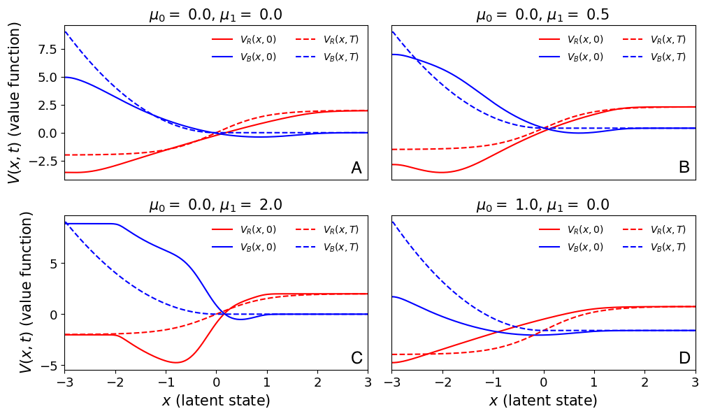
Figure 14: We demonstrate the lack of qualitative changes in the value functions given by solutions to Eqs. 52 and 53 when compared to the solutions of Eqs. 11 and 12. We plot $V_{i}(x,0)$ in solid curves and $V_{i}(x,T)$ in dashed curves, $i\in\{\mathrm{R},\mathrm{B}\}$. We set final conditions here to $\Phi_{\mathrm{R}}(x)=\tanh x$ and $\Phi_{\mathrm{B}}(x)=\frac{1}{2}x^{2}\Theta(-x)$.

With the modification of Eq. 51, Red’s HJB equation reads

$$-\frac{\partial V_{\mathrm{R}}}{\partial t}=-\frac{1}{4}\left(\frac{\partial V_{\mathrm{R}}}{\partial x}\right)^{2}-\frac{1}{2}\frac{\partial V_{\mathrm{R}}}{\partial x}\frac{\partial V_{\mathrm{B}}}{\partial x}$$ (54)

$$-\frac{\lambda_{\mathrm{R}}}{4}\left(\frac{\partial V_{\mathrm{B}}}{\partial x}\right)^{2}-\Theta(-x)+\frac{\sigma^{2}}{2}\frac{\partial^{2}V_{\mathrm{R}}}{\partial x^{2}},$$

$$\qquad V_{\mathrm{R}}(x,T)=\Phi_{\mathrm{R}}(x).$$

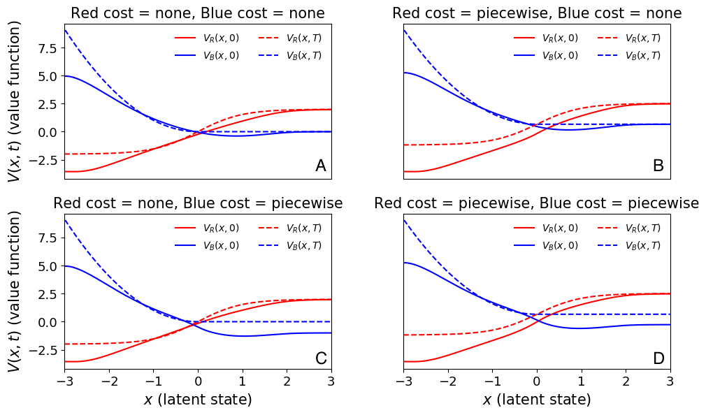
Figure 15: We demonstrate the lack of qualitative changes in the value functions given by the solution to Eqs. 54 when compared to the solutions of Eqs. 11 and 12. We plot $V_{i}(x,0)$ in solid curves and $V_{i}(x,T)$ in dashed curves, $i\in\{\mathrm{R},\mathrm{B}\}$. We set final conditions here to $\Phi_{\mathrm{R}}(x)=\tanh x$ and $\Phi_{\mathrm{B}}(x)=\frac{1}{2}x^{2}\Theta(-x)$. We also plot solutions for an augmented HJB equation for Blue in panels C and D. This HJB equation is identical to Eq. 54 except with $\mathrm{R}\mapsto\mathrm{B}$ and the sign of argument of the discontinuous running cost function reversed.

We plot solutions of Eq. 54 in Fig. 15. These solutions also do not change qualitatively from the solutions to Eqs. 11 and 12 in that there is no shock or travelling wave formation . A more fundamental qualitative change would be to expand the scope of Red’s interference to alter the latent volatility of the election process. Red’s additional objective might be to increase the uncertainty in polling results.

In addition to theoretical modifications, other work could extend these results to other elections using similarly fine-grained or more granular data. This approach is difficult because there is very little granular public data on election interference levin2019partisan . We are able to confront our model to data only because the Russian interference in the 2016 U.S. presidential election was well-publicized and because the interference took place at least partially through the mechanism of Twitter, which is a public data source. We were unable to find any other publicly-available data at daily (or finer) temporal resolution for any other publicly-acknowledged election interference episode.

In the case study of the 2016 U.S. presidential election, our theoretical model accurately captured election interference dynamics from approximately two weeks after the Democratic National Convention until Election Day. However, it did not capture the dynamics of election interference accurately or precisely during the first fortnight of time under study. We believe this is because, even though the election was then a two-candidate contest, there were additional election state and interference dynamics that we did not model. We believe that these dynamics arise because the transition from interfering in many candidates’ primary campaigns to interfering in only one electoral contest is not immediate. It likely takes time for the foreign intelligence agency to recalibrate their interference strategy. In addition, the foreign intelligence agency may still expend reseources on influencing other candidates’ supporters, even though those other candidates had been unsuccessful in their quest for inclusion in the general election. Suppose that there are initially $N_{\mathrm{R}}$ “red candidates” (candidates that the foreign intelligence service would like to win the election) and $N_{\mathrm{B}}$ “blue candidates” (candidates that the foreign intelligence service would not like to win the election). Then modeling the transition between the conventions and the general election requires collapsing the state equation from a $N_{\mathrm{R}}+N_{\mathrm{B}}-2$-dimensional stochastic differential equation (SDE) to a one-dimensional SDE. The cost functions of Red and Blue would probably also change during this transition, but we are unsure of how to model this change. Because of the dimensionality reduction in the state equation, the coupled HJB equations would change from being PDEs solved in $N_{\mathrm{R}}+N_{\mathrm{B}}-2$ spatial dimensions to ones solved in one spatial dimension, as now. We did not attempt to model these dynamics, but this could be a useful expansion of our model.

We used two models in our analysis of interference in the 2016 U.S. presidential election. We used a Bayesian structural time series model to infer the latent random variables $u_{\mathrm{R}}$, $u_{\mathrm{B}}$, and $X$, and then used these inferred values to fit parameters of the theoretical model described in Sec. II.2. While the theoretical model does not have many free parameters ($2K+3=23$ degrees of freedom), the structural time series model does have many free parameters ($3T+5=311$ degrees of freedom). The large number of free parameters of the structural time series model does not mean that the model is overparameterized. At each $t$, we observe a number of tweets $\text{Tweets}_{t}$ and a popularity rating for the candidates $Z_{t}$. From these we want to infer the distributions of the random variables $u_{\mathrm{R},t}$, $u_{\mathrm{B},t}$, and $X_{t}$. Since we want to infer the distribution of each of these three random variables at each of the $T$ timesteps, this large number of parameters is expressly necessary. If we observe $M$ identical trials of an election process over $T$ timesteps, the ratio of structural time series model parameters to observed datapoints is given by

$$R(T,M)=\frac{3T+5}{2MT}=\frac{3}{2}M^{-1}\left(1+\frac{5}{3}T^{-1}\right).$$ (55)

With $T$ held constant, $R(T,M)\rightarrow 0$ as $M$ grows, while with $M$ held constant, $R(T,M)\rightarrow\frac{3}{2}$ as $T$ grows large. Since we observe only one draw from the election interference model, $M=1$ in our case. However, this approach of inferring each random variable’s distribution is not tractable when $T$ becomes large since the number of parameters to fit still grows linearly with $T$.

One way of partially circumventing this problem is to use a variational inference approach combined with amortization of the random variables. Denote the vector of all observed random variables at time $t$ by $y_{t}$ and the vector of all latent random variables at time $t$ by $w_{t}$. Variational inference replaces the actual posterior distribution with an approximate posterior distribution that has a known normalization constant (thereby eliminating the need for MCMC routines to compute this constant) hoffman2013stochastic ; rezende2015variational ; blei2017variational . The parameters of the approximate posterior are found through optimization, which is generally much faster than Monte Carlo sampling. If the joint distribution of $y=(y_{1},...,y_{T})$ and $w=(w_{1},...,w_{T})$ is given by $p(y,w)=\prod_{t=1}^{T}p(y_{t}|w_{t})p(w_{t})$, then the true posterior is given by $p(w|y)=p(y,w)/p(y)$. The approximate (variational) posterior is given by $q_{\theta}(w)=\prod_{t=1}^{T}q_{\theta_{t}}(w_{t})$, where $\theta=(\theta_{1},...,\theta_{T})$ is the vector of parameters found through optimization and $q_{\theta_{t}}(w_{t})$ are the probability distributions for each timestep. The normalizing constants are known for each $q_{\theta_{t}}(w_{t})$.

Amortization of the random variables means that, instead of finding the optimal value of the entire length-$T$ vector $\theta$, we model the approximate posterior as $q_{\psi}(w)=\prod_{t=1}^{T}q(w_{t}|f_{\psi}(y_{t}))$ rezende2015variational ; zhang2018advances . The vector $\psi$ is the vector of parameters of the (probably nonlinear) function $f_{\psi}(\cdot)$ and does not scale with $T$. The function $f_{\psi}(\cdot)$ models the effect of the time-dependent parameters $\theta_{t}$ of the variational posterior. This amortized variational posterior is also fit using an optimization routine. Since the number of parameters of this model does not scale with time, Eq. 55 for this model becomes

$$R_{\text{amort}}(T,M)=\frac{P}{2MT},$$ (56)

where $P$ is the constant number of parameters (the dimension of $\psi$) in the amortized model. For fixed $M$, $R_{\text{amort}}(M,T)\rightarrow 0$ as $T$ becomes large. Another useful extension of our present work would be to reimplement our Bayesian structural time series model using amortized variational inference. This would also eliminate the problem of choosing the “correct” number of parameters in the Legendre polynomial approximation that we described in Sec. III.

Appendix A Coupling parameter sweeps

We conducted parameter sweeps over different values of the coupling parameters $\lambda_{\mathrm{R}}$ and $\lambda_{\mathrm{B}}$ for multiple combinations of Red and Blue final conditions. To do this, we integrated Eqs. 11 and 12 for $\lambda_{\mathrm{R}},\lambda_{\mathrm{B}}\in[0,3]$ for each of the $3^{2}=9$ combinations of the final conditions

$$\Phi_{\mathrm{R}}(x)\in\left\{x,2\tanh x,\Theta(x)-\Theta(-x)\right\}$$ (57)

and

$$\Phi_{\mathrm{B}}(x)\in\left\{\frac{1}{2}x^{2},\frac{1}{2}x^{2}\Theta(-x),2[\Theta(|x|-\Delta)-\Theta(\Delta-|x|)]\right\}.$$ (58)

We integrated Eqs. 11 and 12 for $N_{t}=8000$ timesteps, setting $t_{0}=0$ and $T=1$ year. We enforced Neumann boundary conditions on the interval $x\in[-3,3]$ and set the spatial step size to be $\textnormal{d}x=0.025$. After integration, we then drew $1000$ paths $u_{\mathrm{R}}^{(n)}$ and $u_{\mathrm{B}}^{(n)}$ from the resulting probability distribution over control policies. (This probability distribution is a time-dependent multivariate Gaussian, since the control policies are deterministic functions of the random variable defined by the Ito stochastic differential equation Eq. 3.) We then calculated the intertemporal means and standard deviations of these control policies, which we denote by

$$\text{mean}(u_{i})=\frac{1}{TN}\sum_{n=1}^{N}\int_{0}^{T}u_{i}^{(n)}(t)\ \textnormal{d}t$$ (59)

and

$$\text{std}(u_{i})=\sqrt{\frac{1}{TN}\sum_{n=1}^{N}\int_{0}^{T}\left[u_{i}^{(n)}(t)-\text{mean}(u_{i})\right]^{2}\ \textnormal{d}t},$$ (60)

for $i\in\{\mathrm{R},\mathrm{B}\}$. We display the mean control policies in Sec. A.1 and the standard deviations of the control policies in Sec. A.2.

A.1 Expected value of $u_{i}(t)$

We display the mean paths of draws from the distributions of control policies generated by solutions to Eqs. 11 and 12.

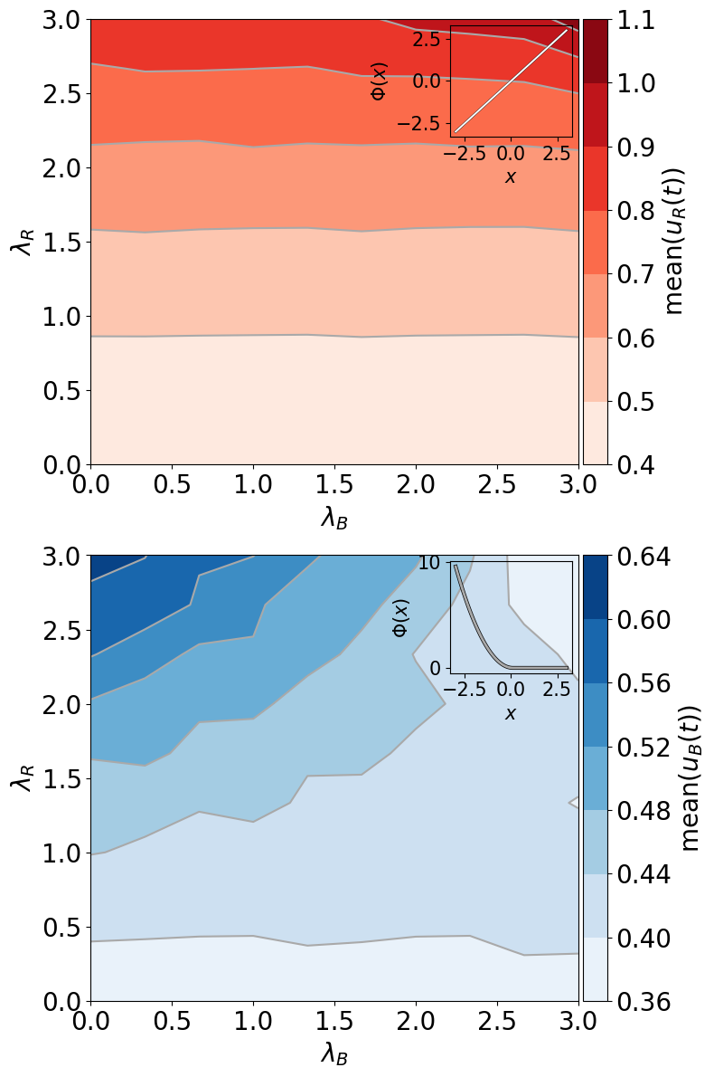
Figure 16: Parameter sweep over coupling parameters $\lambda_{\mathrm{R}},\lambda_{\mathrm{B}}$ with Red final condition $\Phi_{\mathrm{R}}(x)=$ $x$ and Blue final condition $\Phi_{\mathrm{B}}(x)=$ $\frac{1}{2}x^{2}\Theta(-x)$. Intensity of color corresponds to mean of control policy.

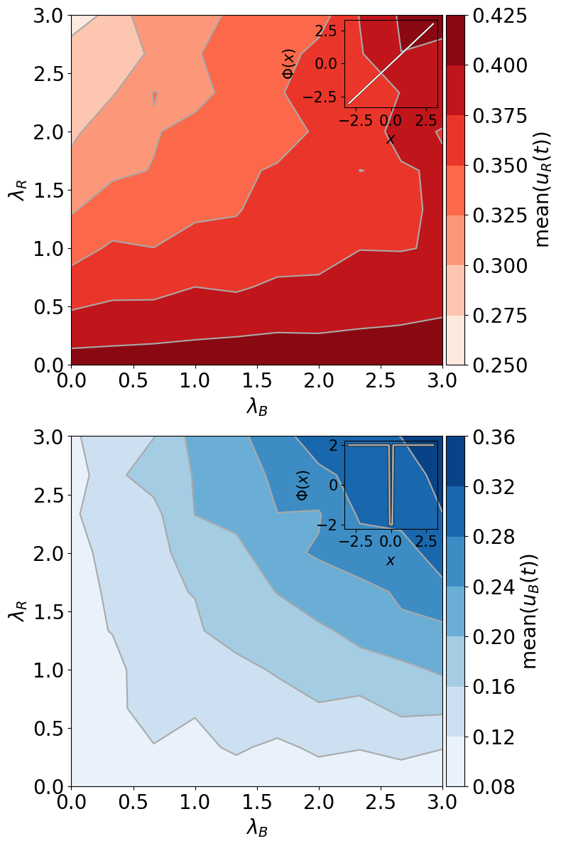
Figure 17: Parameter sweep over coupling parameters $\lambda_{\mathrm{R}},\lambda_{\mathrm{B}}$ with Red final condition $\Phi_{\mathrm{R}}(x)=$ $x$ and Blue final condition $\Phi_{\mathrm{B}}(x)=$ $2[\Theta(|x|-0.1)-\Theta(0.1-|x|)]$. Intensity of color corresponds to mean of control policy.

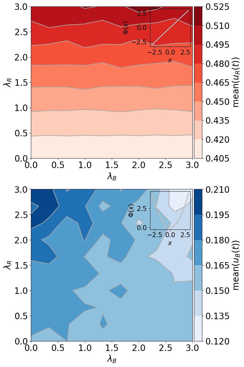
Figure 18: Parameter sweep over coupling parameters $\lambda_{\mathrm{R}},\lambda_{\mathrm{B}}$ with Red final condition $\Phi_{\mathrm{R}}(x)=$ $x$ and Blue final condition $\Phi_{\mathrm{B}}(x)=$ $\frac{1}{2}x^{2}$. Intensity of color corresponds to mean of control policy.

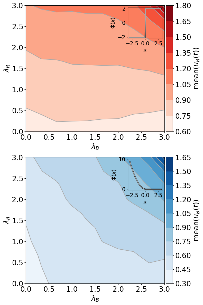
Figure 19: Parameter sweep over coupling parameters $\lambda_{\mathrm{R}},\lambda_{\mathrm{B}}$ with Red final condition $\Phi_{\mathrm{R}}(x)=$ $2[\Theta(x)-\Theta(-x)]$ and Blue final condition $\Phi_{\mathrm{B}}(x)=$ $\frac{1}{2}x^{2}\Theta(-x)$. Intensity of color corresponds to mean of control policy.

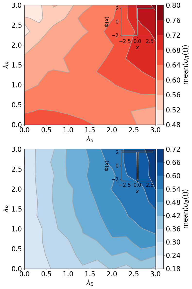
Figure 20: Parameter sweep over coupling parameters $\lambda_{\mathrm{R}},\lambda_{\mathrm{B}}$ with Red final condition $\Phi_{\mathrm{R}}(x)=$ $2[\Theta(x)-\Theta(-x)]$ and Blue final condition $\Phi_{\mathrm{B}}(x)=$ $2[\Theta(|x|-0.1)-\Theta(0.1-|x|)]$. Intensity of color corresponds to mean of control policy.

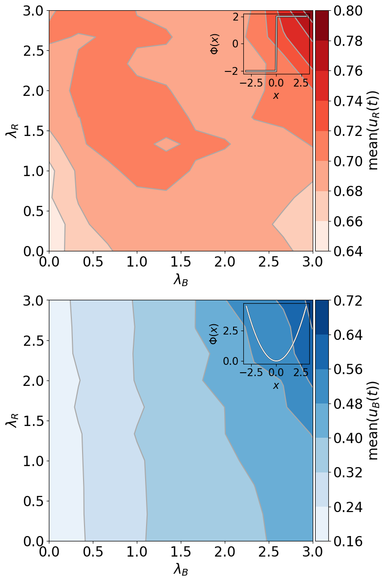
Figure 21: Parameter sweep over coupling parameters $\lambda_{\mathrm{R}},\lambda_{\mathrm{B}}$ with Red final condition $\Phi_{\mathrm{R}}(x)=$ $2[\Theta(x)-\Theta(-x)]$ and Blue final condition $\Phi_{\mathrm{B}}(x)=$ $\frac{1}{2}x^{2}$. Intensity of color corresponds to mean of control policy.

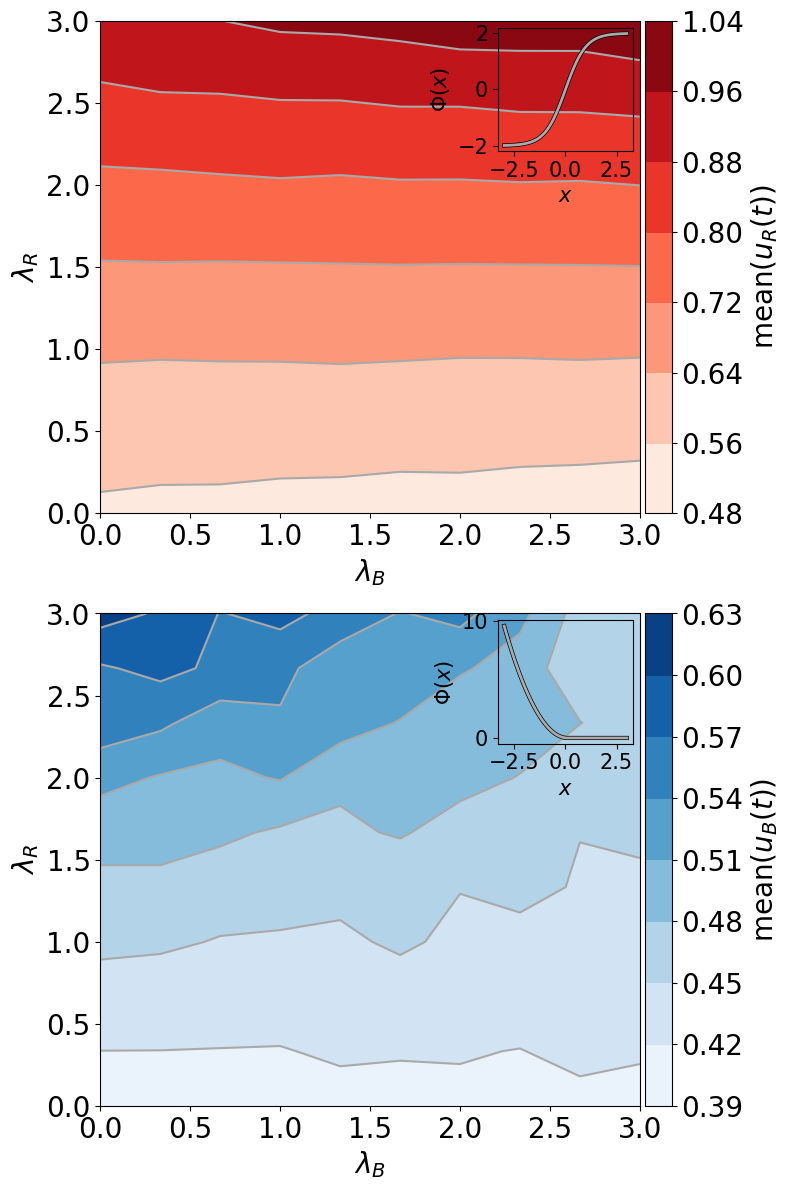
Figure 22: Parameter sweep over coupling parameters $\lambda_{\mathrm{R}},\lambda_{\mathrm{B}}$ with Red final condition $\Phi_{\mathrm{R}}(x)=$ $\tanh(x)$ and Blue final condition $\Phi_{\mathrm{B}}(x)=$ $\frac{1}{2}x^{2}\Theta(-x)$. Intensity of color corresponds to mean of control policy.

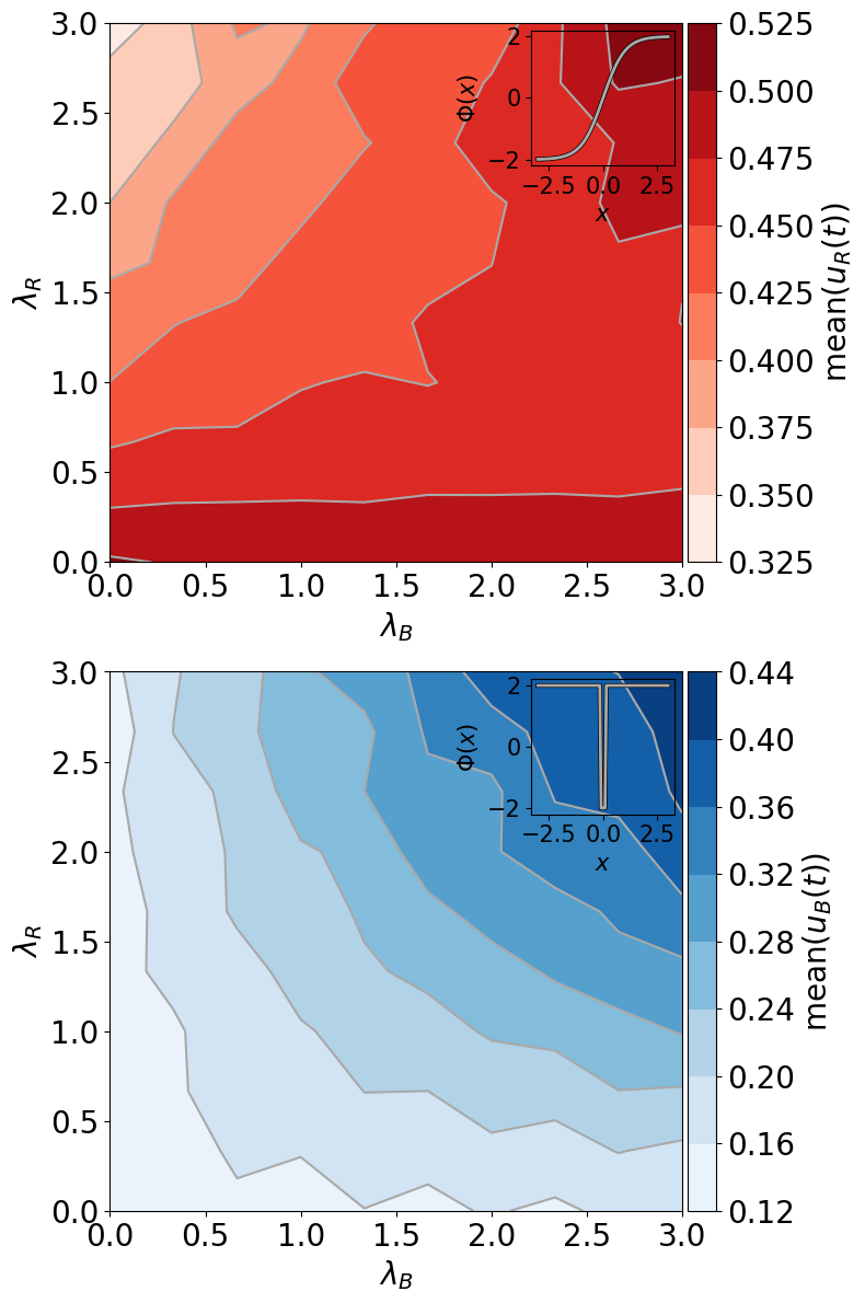
Figure 23: Parameter sweep over coupling parameters $\lambda_{\mathrm{R}},\lambda_{\mathrm{B}}$ with Red final condition $\Phi_{\mathrm{R}}(x)=$ $\tanh(x)$ and Blue final condition $\Phi_{\mathrm{B}}(x)=$ $2[\Theta(|x|-0.1)-\Theta(0.1-|x|)]$. Intensity of color corresponds to mean of control policy.

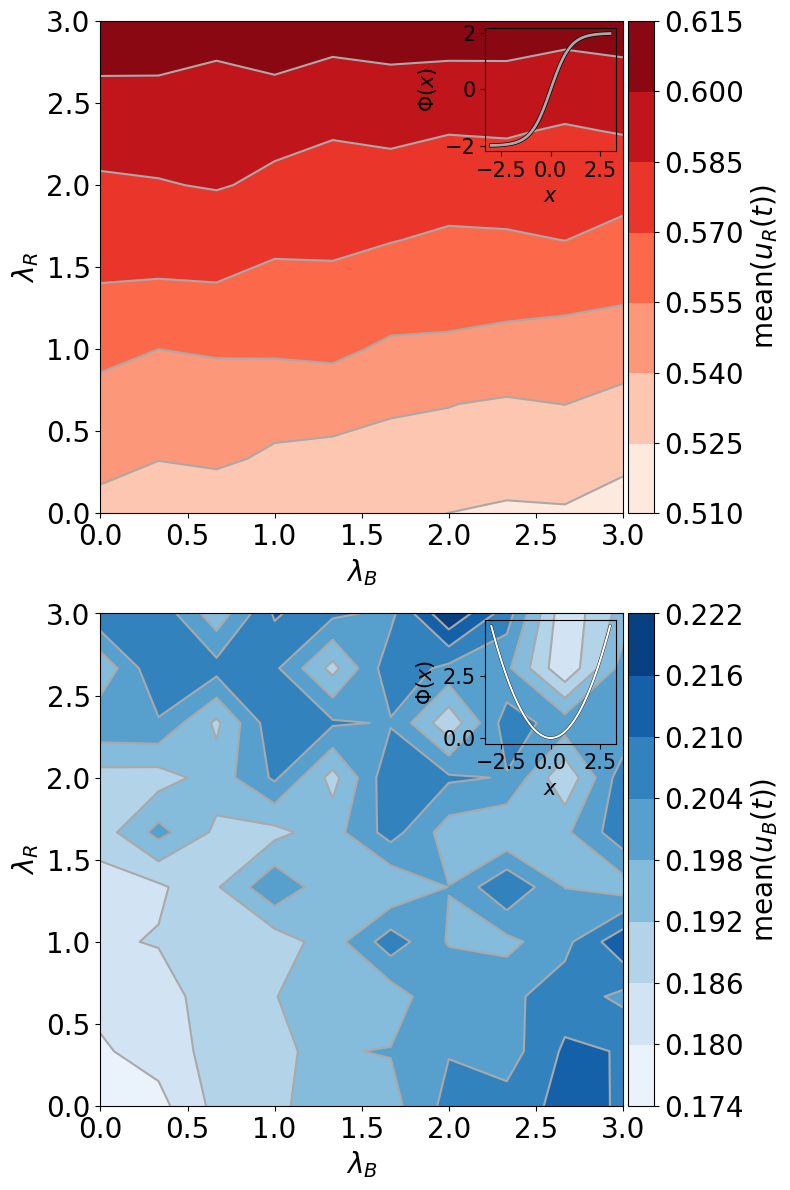
Figure 24: Parameter sweep over coupling parameters $\lambda_{\mathrm{R}},\lambda_{\mathrm{B}}$ with Red final condition $\Phi_{\mathrm{R}}(x)=$ $\tanh(x)$ and Blue final condition $\Phi_{\mathrm{B}}(x)=$ $\frac{1}{2}x^{2}$. Intensity of color corresponds to mean of control policy.

A.2 Standard deviation of $u_{i}(t)$

We display the standard deviation of draws from the distributions of control policies generated by solutions to Eqs. 11 and 12.

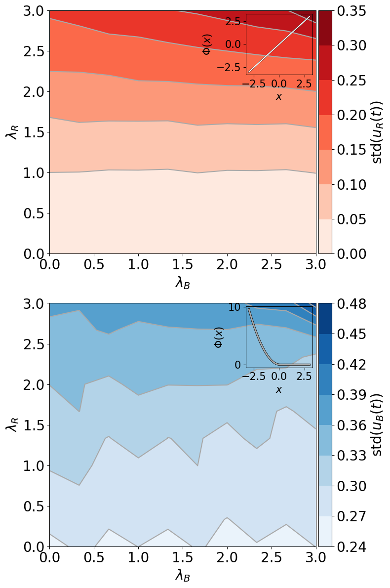
Figure 25: Parameter sweep over coupling parameters $\lambda_{\mathrm{R}},\lambda_{\mathrm{B}}$ with Red final condition $\Phi_{\mathrm{R}}(x)=$ $x$ and Blue final condition $\Phi_{\mathrm{B}}(x)=$ $\frac{1}{2}x^{2}\Theta(-x)$. Intensity of color corresponds to std of control policy.

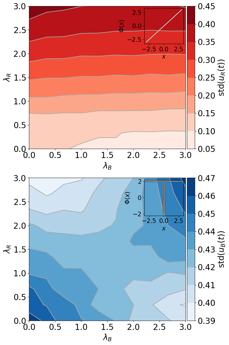
Figure 26: Parameter sweep over coupling parameters $\lambda_{\mathrm{R}},\lambda_{\mathrm{B}}$ with Red final condition $\Phi_{\mathrm{R}}(x)=$ $x$ and Blue final condition $\Phi_{\mathrm{B}}(x)=$ $2[\Theta(|x|-0.1)-\Theta(0.1-|x|)]$. Intensity of color corresponds to std of control policy.

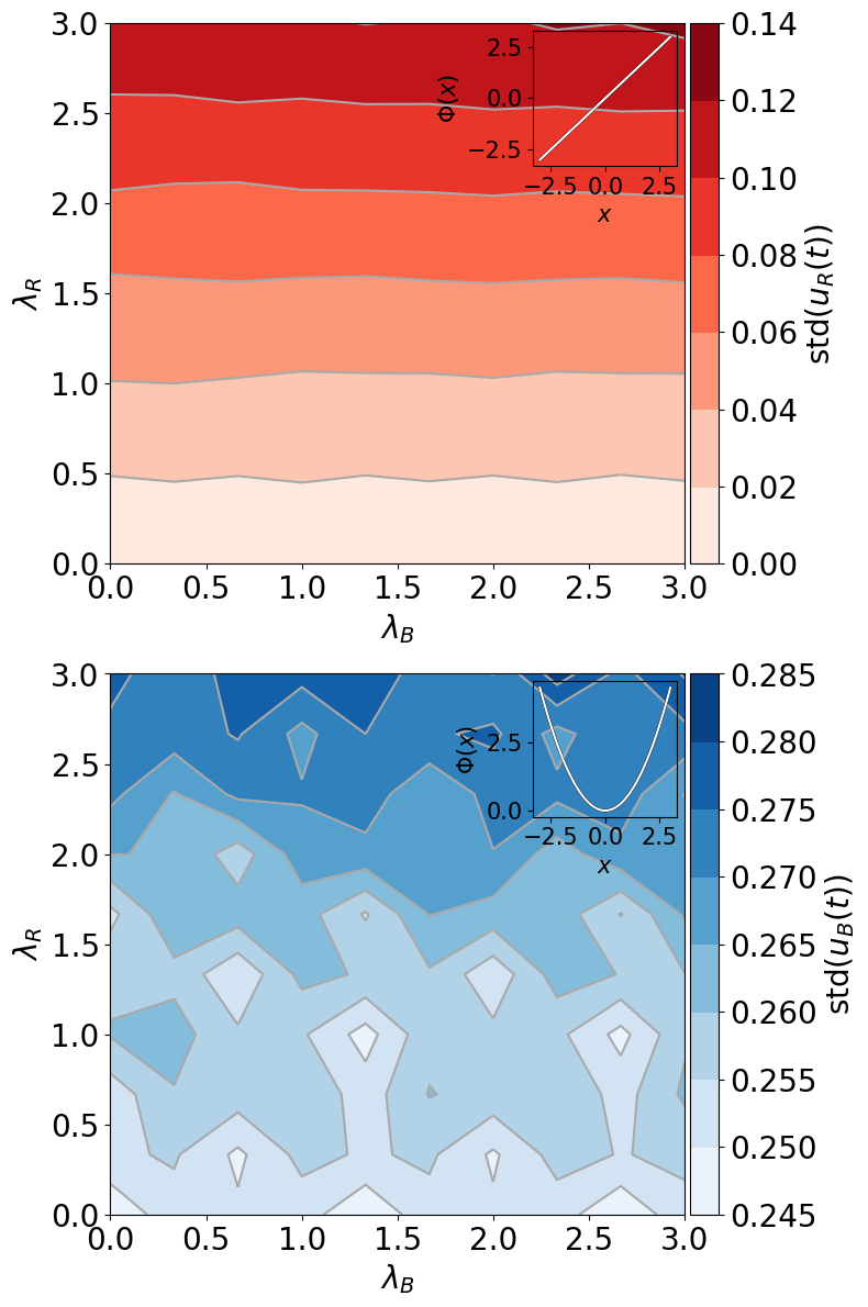
Figure 27: Parameter sweep over coupling parameters $\lambda_{\mathrm{R}},\lambda_{\mathrm{B}}$ with Red final condition $\Phi_{\mathrm{R}}(x)=$ $x$ and Blue final condition $\Phi_{\mathrm{B}}(x)=$ $\frac{1}{2}x^{2}$. Intensity of color corresponds to std of control policy.

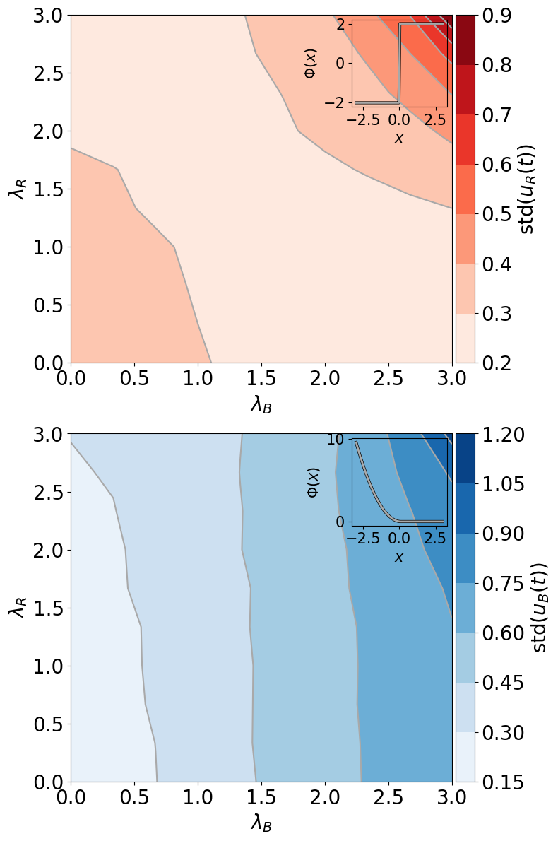
Figure 28: Parameter sweep over coupling parameters $\lambda_{\mathrm{R}},\lambda_{\mathrm{B}}$ with Red final condition $\Phi_{\mathrm{R}}(x)=$ $2[\Theta(x)-\Theta(-x)]$ and Blue final condition $\Phi_{\mathrm{B}}(x)=$ $\frac{1}{2}x^{2}\Theta(-x)$. Intensity of color corresponds to std of control policy.

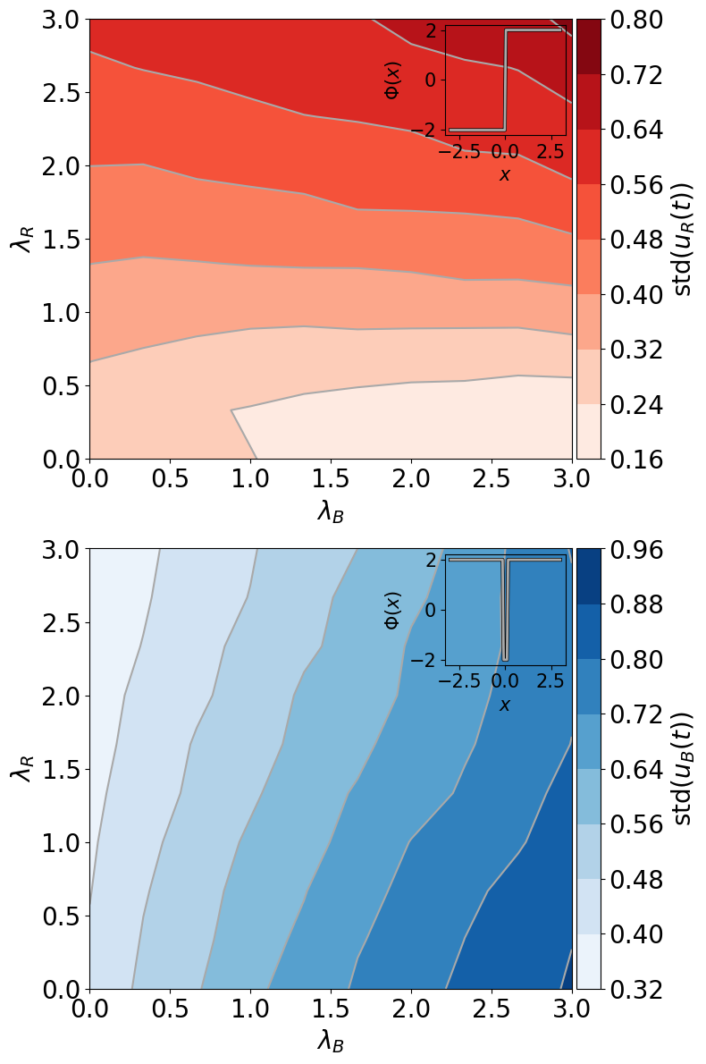
Figure 29: Parameter sweep over coupling parameters $\lambda_{\mathrm{R}},\lambda_{\mathrm{B}}$ with Red final condition $\Phi_{\mathrm{R}}(x)=$ $2[\Theta(x)-\Theta(-x)]$ and Blue final condition $\Phi_{\mathrm{B}}(x)=$ $2[\Theta(|x|-0.1)-\Theta(0.1-|x|)]$. Intensity of color corresponds to std of control policy.

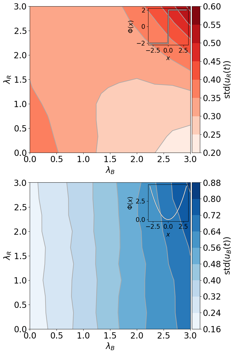
Figure 30: Parameter sweep over coupling parameters $\lambda_{\mathrm{R}},\lambda_{\mathrm{B}}$ with Red final condition $\Phi_{\mathrm{R}}(x)=$ $2[\Theta(x)-\Theta(-x)]$ and Blue final condition $\Phi_{\mathrm{B}}(x)=$ $\frac{1}{2}x^{2}$. Intensity of color corresponds to std of control policy.

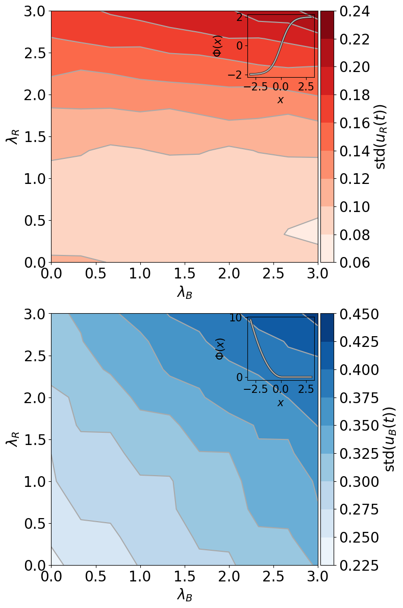
Figure 31: Parameter sweep over coupling parameters $\lambda_{\mathrm{R}},\lambda_{\mathrm{B}}$ with Red final condition $\Phi_{\mathrm{R}}(x)=$ $\tanh(x)$ and Blue final condition $\Phi_{\mathrm{B}}(x)=$ $\frac{1}{2}x^{2}\Theta(-x)$. Intensity of color corresponds to std of control policy.

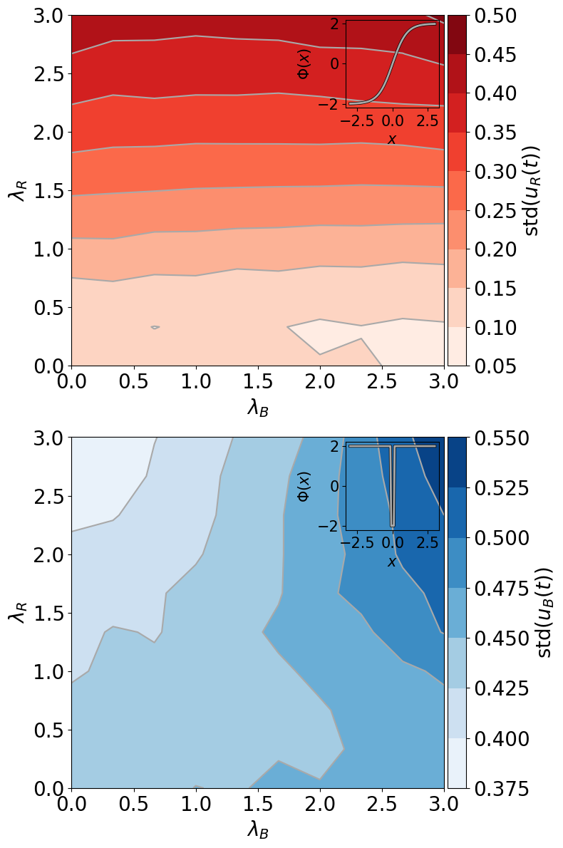
Figure 32: Parameter sweep over coupling parameters $\lambda_{\mathrm{R}},\lambda_{\mathrm{B}}$ with Red final condition $\Phi_{\mathrm{R}}(x)=$ $\tanh(x)$ and Blue final condition $\Phi_{\mathrm{B}}(x)=$ $2[\Theta(|x|-0.1)-\Theta(0.1-|x|)]$. Intensity of color corresponds to std of control policy.

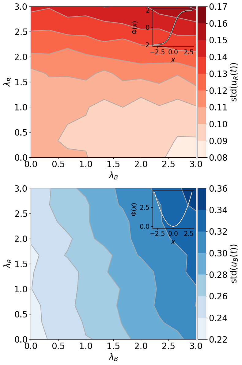
Figure 33: Parameter sweep over coupling parameters $\lambda_{\mathrm{R}},\lambda_{\mathrm{B}}$ with Red final condition $\Phi_{\mathrm{R}}(x)=$ $\tanh(x)$ and Blue final condition $\Phi_{\mathrm{B}}(x)=$ $\frac{1}{2}x^{2}$. Intensity of color corresponds to std of control policy.

References

- (1) Paul SA Renaud and Frans AAM van Winden. On the importance of elections and ideology for government policy in a multi-party system. In The Logic of Multiparty Systems, pages 191–207. Springer, 1987.
- (2) Jorgen Elklit and Palle Svensson. What makes elections free and fair? Journal of Democracy, 8(3):32–46, 1997.
- (3) Dov H Levin. When the great power gets a vote: The effects of great power electoral interventions on election results. International Studies Quarterly, 60(2):189–202, 2016.
- (4) Stephen Shulman and Stephen Bloom. The legitimacy of foreign intervention in elections: The ukrainian response. Review of International Studies, 38(2):445–471, 2012.
- (5) Daniel Corstange and Nikolay Marinov. Taking sides in other people’s elections: The polarizing effect of foreign intervention. American Journal of Political Science, 56(3):655–670, 2012.
- (6) Dov H Levin. Partisan electoral interventions by the great powers: Introducing the PEIG Dataset. Conflict Management and Peace Science, 36(1):88–106, 2019.
- (7) Erica D Borghard and Shawn W Lonergan. Confidence Building Measures for the Cyber Domain. Strategic Studies Quarterly, 12(3):10–49, 2018.
- (8) Dov H Levin. Voting for Trouble? Partisan Electoral Interventions and Domestic Terrorism. Terrorism and Political Violence, pages 1–17, 2018.
- (9) Isabella Hansen and Darren J Lim. Doxing democracy: influencing elections via cyber voter interference. Contemporary Politics, 25(2):150–171, 2019.
- (10) Johannes Bubeck, Kai Jäger, Nikolay Marinov, and Federico Nanni. Why Do States Intervene in the Elections of Others? Available at SSRN 3435138, 2019.
-
(11)
Read the Mueller Report: Searchable Document and Index:
https://www.nytimes.com/interactive
/2019/04/18/us/politics/mueller-report-document.html. New York Times, Apr 2019. - (12) Charles R Nelson and Charles R Plosser. Trends and random walks in macroeconmic time series: some evidence and implications. Journal of monetary economics, 10(2):139–162, 1982.
- (13) David N DeJong, John C Nankervis, N Eugene Savin, and Charles H Whiteman. Integration versus trend stationary in time series. Econometrica: Journal of the Econometric Society, pages 423–433, 1992.
- (14) Crispin W Gardiner. Handbook of Stochastic Methods, volume 3. Springer Berlin, 1985.
- (15) Peter Jung and Peter Hänggi. Dynamical systems: a unified colored-noise approximation. Physical Review A, 35(10):4464, 1987.
- (16) Peter Hänggi and Peter Jung. Colored noise in dynamical systems. Advances in Chemical Physics, 89:239–326, 1995.
- (17) Richard Bellman. Dynamic programming and a new formalism in the calculus of variations. Proceedings of the National Academy of Sciences of the United States of America, 40(4):231, 1954.
- (18) Richard Bellman. Dynamic programming. Science, 153(3731):34–37, 1966.
- (19) Richard S Sutton and Andrew G Barto. Reinforcement learning: An introduction. MIT press, 2018.
- (20) Hilbert J Kappen. An introduction to stochastic control theory, path integrals and reinforcement learning. In AIP conference proceedings, volume 887, pages 149–181. AIP, 2007.
- (21) Karl J Åström. Introduction to stochastic control theory. Courier Corporation, 2012.
- (22) Tryphon T Georgiou and Anders Lindquist. The separation principle in stochastic control, redux. IEEE Transactions on Automatic Control, 58(10):2481–2494, 2013.
- (23) Ernst Zermelo. Über eine anwendung der mengenlehre auf die theorie des schachspiels. In Proceedings of the fifth international congress of mathematicians, volume 2, pages 501–504. Cambridge University Press Cambridge, UK, 1913.
- (24) John Nash. Non-cooperative games. Annals of mathematics, pages 286–295, 1951.
- (25) Drew Fudenberg and Jean Tirole. Noncooperative game theory for industrial organization: an introduction and overview. Handbook of industrial Organization, 1:259–327, 1989.
- (26) Andreu Mas-Colell, Michael Dennis Whinston, Jerry R Green, et al. Microeconomic theory, volume 1. Oxford university press New York, 1995.
- (27) Rainer Buckdahn and Juan Li. Stochastic differential games and viscosity solutions of Hamilton–Jacobi–Bellman–Isaacs equations. SIAM Journal on Control and Optimization, 47(1):444–475, 2008.
- (28) Triet Pham and Jianfeng Zhang. Two person zero-sum game in weak formulation and path dependent Bellman–Isaacs equation. SIAM Journal on Control and Optimization, 52(4):2090–2121, 2014.
- (29) Code to recreate simulations and plots in this paper, or to create new simulations and “what-if” scenarios, is located at https://gitlab.com/daviddewhurst/red-blue-game.
- (30) There is a large literature on nonparametric functional approximation that we cannot review here. Here is an example of this type of approximation. If is any partition of and the vector were jointly distributed Gaussian on , then we say that and are distributed according to a Gaussian process williams2006gaussian. Though this infinite-dimensional formalism can be useful when deriving theoretical results, in practice we would approximate this process by a finite-dimensional multivariate Gaussian. In Sec. III we actually approximate and by finite sums of Legendre polynomials and infer the coefficients of these polynomials as our multivariate approximation.
- (31) Ming-Hui Chen and Qi-Man Shao. Monte carlo estimation of bayesian credible and hpd intervals. Journal of Computational and Graphical Statistics, 8(1):69–92, 1999.
- (32) Valery E Yarynich. C3: nuclear command, control cooperation. Center for Defense Information, 2003.
- (33) Anthony M Barrett. False alarms, true dangers? RAND Corporation document PE-191-TSF, DOI, 10, 2016.
- (34) Hilbert J Kappen. Path integrals and symmetry breaking for optimal control theory. Journal of Statistical Mechanics: Theory and Experiment, 2005(11):P11011, 2005.
- (35) Mark Kac. On distributions of certain Wiener functionals. Transactions of the American Mathematical Society, 65(1):1–13, 1949.
- (36) Yaming Chen, Adrian Baule, Hugo Touchette, and Wolfram Just. Weak-noise limit of a piecewise-smooth stochastic differential equation. Physical Review E, 88(5):052103, 2013.
- (37) Julie Leifeld, Kaitlin Hill, and Andrew Roberts. Persistence of saddle behavior in the nonsmooth limit of smooth dynamical systems. arXiv preprint arXiv:1504.04671, 2015.
- (38) Kiyoshi Kanazawa, Tomohiko G Sano, Takahiro Sagawa, and Hisao Hayakawa. Asymptotic derivation of Langevin-like equation with non-gaussian noise and its analytical solution. Journal of Statistical Physics, 160(5):1294–1335, 2015.
- (39) Sofia H Piltz, Lauri Harhanen, Mason A Porter, and Philip K Maini. Inferring parameters of prey switching in a 1 predator–2 prey plankton system with a linear preference tradeoff. Journal of Theoretical Biology, 456:108–122, 2018.
- (40) Peter Tanchak. The Invisible Front: Russia, Trolls, and the Information War against Ukraine. Revolution and War in Contemporary Ukraine: The Challenge of Change, 161:253, 2017.
- (41) Brandon C Boatwright, Darren L Linvill, and Patrick L Warren. Troll factories: The internet research agency and state-sponsored agenda building. Resource Centre on Media Freedom in Europe, 2018.
- (42) Adam Badawy, Emilio Ferrara, and Kristina Lerman. Analyzing the digital traces of political manipulation: the 2016 Russian interference Twitter campaign. In 2018 IEEE/ACM International Conference on Advances in Social Networks Analysis and Mining (ASONAM), pages 258–265. IEEE, 2018.
- (43) Ryan L Boyd, Alexander Spangher, Adam Fourney, Besmira Nushi, Gireeja Ranade, James Pennebaker, and Eric Horvitz. Characterizing the Internet Research Agency’s Social Media Operations During the 2016 US Presidential Election using Linguistic Analyses. 2018.
- (44) Damian J Ruck, Natalie M Rice, Joshua Borycz, and R Alexander Bentley. Internet Research Agency Twitter activity predicted 2016 US election polls. First Monday, 24(7), 2019.
- (45) Nicolas Guenon des Mesnards and Tauhid Zaman. Detecting influence campaigns in social networks using the Ising model. arXiv preprint arXiv:1805.10244, 2018.
- (46) Jane Im, Eshwar Chandrasekharan, Jackson Sargent, Paige Lighthammer, Taylor Denby, Ankit Bhargava, Libby Hemphill, David Jurgens, and Eric Gilbert. Still out there: Modeling and Identifying Russian Troll Accounts on Twitter. arXiv preprint arXiv:1901.11162, 2019.
- (47) Alexandria Volkening, Daniel F Linder, Mason A Porter, and Grzegorz A Rempala. Forecasting elections using compartmental models of infections. arXiv preprint arXiv:1811.01831, 2018.
- (48) David Rothschild. Forecasting elections: Comparing prediction markets, polls, and their biases. Public Opinion Quarterly, 73(5):895–916, 2009.
- (49) Drew A Linzer. Dynamic Bayesian forecasting of presidential elections in the states. Journal of the American Statistical Association, 108(501):124–134, 2013.
- (50) Wei Wang, David Rothschild, Sharad Goel, and Andrew Gelman. Forecasting elections with non-representative polls. International Journal of Forecasting, 31(3):980–991, 2015.
- (51) Data can be downloaded at https://github.com/fivethirtyeight/russian-troll-tweets/.
- (52) Ramin Skibba. Pollsters struggle to explain failures of us presidential forecasts. Nature News, 539(7629):339, 2016.
- (53) Ryan Neville-Shepard. Constrained by duality: Third-party master narratives in the 2016 presidential election. American Behavioral Scientist, 61(4):414–427, 2017.
- (54) Data can be downloaded at https://www.realclearpolitics.com/epolls/2016/president/us/general_election_trump_vs_clinton_vs_johnson_vs_stein-5952.html.
- (55) David Barber, A Taylan Cemgil, and Silvia Chiappa. Bayesian Time Series Models. Cambridge University Press, 2011.
- (56) Agner Krarup Erlang. Sandsynlighedsregning og telefonsamtaler. Nyt tidsskrift for Matematik, 20:33–39, 1909.
- (57) Georg Rasch. The poisson process as a model for a diversity of behavioral phenomena. In International congress of psychology, volume 2, page 2, 1963.
- (58) David R Cox. Regression models and life-tables. Journal of the Royal Statistical Society: Series B (Methodological), 34(2):187–202, 1972.
- (59) David Roxbee Cox and Valerie Isham. Point processes, volume 12. CRC Press, 1980.
- (60) Matthew D Hoffman and Andrew Gelman. The No-U-Turn sampler: adaptively setting path lengths in Hamiltonian Monte Carlo. Journal of Machine Learning Research, 15(1):1593–1623, 2014.
- (61) Andrew Gelman, Donald B Rubin, et al. Inference from iterative simulation using multiple sequences. Statistical Science, 7(4):457–472, 1992.
- (62) Stephen P Brooks and Andrew Gelman. General methods for monitoring convergence of iterative simulations. Journal of Computational and Graphical Statistics, 7(4):434–455, 1998.
- (63) Eric Brochu, Vlad M Cora, and Nando De Freitas. A tutorial on Bayesian optimization of expensive cost functions, with application to active user modeling and hierarchical reinforcement learning. arXiv preprint arXiv:1012.2599, 2010.
- (64) Bobak Shahriari, Kevin Swersky, Ziyu Wang, Ryan P Adams, and Nando De Freitas. Taking the human out of the loop: A review of Bayesian optimization. Proceedings of the IEEE, 104(1):148–175, 2015.
- (65) Peter I Frazier. A tutorial on bayesian optimization. arXiv preprint arXiv:1807.02811, 2018.
- (66) Nassim Nicholas Taleb. Election predictions as martingales: An arbitrage approach. Quantitative Finance, 18(1):1–5, 2018.
- (67) Using the HJB integrator red_blue_pdes.py included in the code at %****␣red-blue-game.bbl␣Line␣400␣****https://gitlab.com/daviddewhurst/red-blue-game, the reader may further investigate the effects of changes in the drift and running cost terms on the qualitative nature of solutions to the coupled HJB system.
- (68) Matthew D Hoffman, David M Blei, Chong Wang, and John Paisley. Stochastic variational inference. The Journal of Machine Learning Research, 14(1):1303–1347, 2013.
- (69) Danilo Jimenez Rezende and Shakir Mohamed. Variational inference with normalizing flows. arXiv preprint arXiv:1505.05770, 2015.
- (70) David M Blei, Alp Kucukelbir, and Jon D McAuliffe. Variational inference: A review for statisticians. Journal of the American statistical Association, 112(518):859–877, 2017.
- (71) Cheng Zhang, Judith Butepage, Hedvig Kjellstrom, and Stephan Mandt. Advances in variational inference. IEEE transactions on pattern analysis and machine intelligence, 2018.