Sulfate Aerosol Hazes and SO2 Gas as Constraints on Rocky Exoplanets’ Surface Liquid Water

Abstract

Despite surface liquid water’s importance to habitability, observationally diagnosing its presence or absence on exoplanets is still an open problem. Inspired within the Solar System by the differing sulfur cycles on Venus and Earth, we investigate thick sulfate (H2SO4-H2O) aerosol haze and high trace mixing ratios of SO2 gas as observable atmospheric features whose sustained existence is linked to the near-absence of surface liquid water. We examine the fundamentals of the sulfur cycle on a rocky planet with an ocean and an atmosphere in which the dominant forms of sulfur are SO2 gas and H2SO4-H2O aerosols (as on Earth and Venus). We build a simple but robust model of the wet, oxidized sulfur cycle to determine the critical amounts of sulfur in the atmosphere-ocean system required for detectable levels of SO2 and a detectable haze layer. We demonstrate that for physically realistic ocean pH values (pH $\gtrsim$ 6) and conservative assumptions on volcanic outgassing, chemistry, and aerosol microphysics, surface liquid water reservoirs with greater than $10^{-3}$ Earth oceans are incompatible with a sustained observable H2SO4-H2O haze layer and sustained observable levels of SO2. Thus, we propose the observational detection of an H2SO4-H2O haze layer and of SO2 gas as two new remote indicators that a planet does not host significant surface liquid water.

1 Introduction

Surface liquid water is considered essential to Earth-like life (e.g., Scalo et al.,, 2007; Kasting,, 2012), so determining whether a planet possesses liquid water is essential to constraining its habitability. As exoplanet detection and characterization techniques improve, observational constraints on the presence of surface water in the form of oceans will be a precursor to building an understanding of the occurrence rate of Earth-like planets and, ultimately, to building an understanding of the occurrence rate of Earth-like life. For many planets, the absence of surface oceans can be determined from straightforward physical arguments. Oceans require a surface temperature and pressure consistent with the stability of liquid water. These requirements limit possible ocean-hosting planet candidates to low-mass ($M\lesssim 10M_{\oplus}$) planets in the habitable zone (e.g., Kasting et al.,, 1993; Kopparapu et al.,, 2013).

While these fundamental requirements can be reasonably evaluated from a planet’s density and received stellar flux, evaluating whether rocky, habitable-zone planets actually possess surface oceans will be a substantial challenge, even for next-generation telescopes. While atmospheric spectra can identify water vapor in a planet’s atmosphere (e.g., Deming et al.,, 2013; Huitson et al.,, 2013; Fraine et al.,, 2014; Sing et al.,, 2016), such a detection says nothing conclusively about surface liquid water. Temporally resolved reflected light spectra can potentially identify the presence of liquid water via color variation due to dark ocean color (Cowan et al.,, 2009), polarized light variation due to ocean smoothness (Zugger et al.,, 2010), and/or ocean glint due to ocean reflectivity (Robinson et al.,, 2010). However, these methods all involve some combination of caveats, including still-unresolved potential false positives, decades-away instrumentation, and a reliance on ideal planetary conditions (Cowan et al.,, 2012). To systematically probe the presence of surface oceans on exoplanets, additional methods will unquestionably be needed. Here, we propose two such methods.

Though all existing ocean detection proposals exploit liquid water’s radiative properties, other planetary-scale implications of the presence of surface liquid water exist. A hydrosphere can substantially alter a planet’s chemistry, including—most notably here—its sulfur cycle. Previous studies of the observability of sulfur in exoplanet atmospheres suggest that sulfur has the capability to be observed in atmospheres in both aerosol and gas species (Kaltenegger and Sasselov,, 2010; Kaltenegger et al.,, 2010; Hu et al.,, 2013; Misra et al.,, 2015; Lincowski et al.,, 2018). In this paper, we test whether the observations of a permanent sulfate (H2SO4-H2O) haze layer and atmospheric SO2 can diagnose the absence of significant surface liquid water. (Note that we do not consider the inverse of this hypothesis—i.e., a lack of observable atmospheric sulfur implies the presence of an ocean—which is not particularly tenable.)

H2SO4-H2O aerosols with sufficient optical depth could be detected in exoplanet atmospheric spectra in the near future (Hu et al.,, 2013; Misra et al.,, 2015). Within the Solar System, Venus and Earth are examples of rocky planets with drastically different surface liquid water volumes and sulfur aerosol opacities. Venus has a global, optically thick H2SO4-H2O aerosol layer (Knollenberg and Hunten,, 1980) and no surface liquid water. Earth, in contrast, only briefly hosts H2SO4-H2O aerosol layers of significant optical depth after large volcanic eruptions (McCormick et al.,, 1995). Earth’s present inability to sustain an H2SO4-H2O aerosol layer in its atmosphere can be directly tied to the presence of oceans, as we show in Section 3.

Beyond aerosols, SO2 gas also has the potential to be detected at $\gtrsim$ 1 ppm mixing ratios (Kaltenegger and Sasselov,, 2010; Hu et al.,, 2013). Previous results have found that building up sulfur concentrations to this level with an Earth-like sulfur cycle requires implausibly high outgassing rates (Kaltenegger et al.,, 2010; Hu et al.,, 2013). We show in Section 3 that the presence of surface liquid water represents a fundamental barrier to maintaining high trace atmospheric sulfur gas levels in such circumstances.

The structure of this paper is as follows. In Section 2, we define the range of planetary atmospheres we consider. Section 3 describes our model of the sulfur cycle on a wet, oxidized world. Section LABEL:sec:results presents the key findings of our model on the incompatibility of observable H2SO4-H2O aerosols and SO2 gas with abundant surface liquid water. In Section 5, we discuss the implications and limitations of this study and make some suggestions for future work. Section 6 summarizes our conclusions.

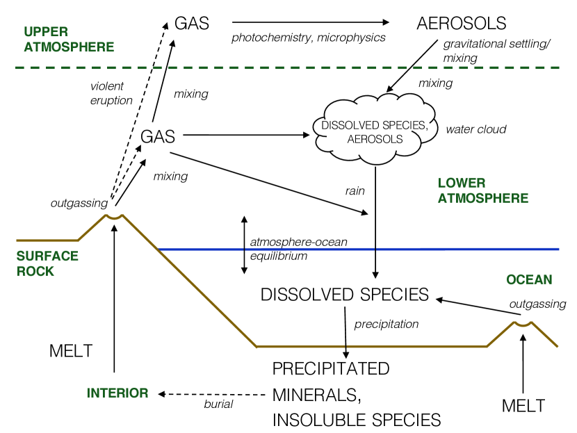
Figure 1: Schematic of the major components of the sulfur cycle on a planet with an ocean and active hydrological cycle.

2 The Sulfur Cycle on Wet, Oxidized Planets

In this paper, we model the sulfur cycle on wet, oxidized planets. We take a wet planet to be a planet with a reservoir of surface liquid water and an active hydrological cycle. We define an oxidized planet based on the atmospheric gas and aerosol sulfur species present, as discussed in further detail below.

Figure 1 summarizes the sulfur cycle on a wet planet. Sulfur gas (SO2 or H2S) is outgassed from melt transported from the interior via volcanism. In the ocean, this gas dissolves, and the aqueous sulfur species are dynamically mixed; in the lower atmosphere, the gas is dynamically mixed. Some gas reaches the upper atmosphere where a series of photochemical reactions produces sulfur gas that condenses into aerosols (H2SO4-H2O or S8, depending on the atmospheric redox state). These aerosols are transported from the upper atmosphere to the lower atmosphere via gravitational settling or mixing on timescales that may depend on the size of the aerosol. Both sulfur gas and aerosols are removed from the lower atmosphere via their interactions with cloud-water and rainwater. Henry’s law dictates an equilibrium between sulfur gas in the atmosphere and aqueous dissolved sulfur species. Further reactions lead to the formation of sulfur minerals, which precipitate out of the ocean when they become saturated. These sediments may eventually be recycled in the interior depending on the planet’s tectonic regime.

Because sulfur can stably occupy a wide range of redox states (commonly -2, 0, +4, +6; or S(-II), S(0), S(IV), S(VI), respectively), the precise sulfur species involved in a planet’s cycle depend on the oxidization state of its interior, atmosphere, and ocean (e.g., Kasting et al.,, 1989; Pavlov and Kasting,, 2002; Johnston,, 2011; Hu et al.,, 2013). Generally, oxidized atmospheres have SO2 gas and form aerosols composed of H2SO4 and H2O, whereas reduced atmospheres have H2S gas and aerosols made of S8 (Hu et al.,, 2013). A planetary system in a more intermediate redox state will have both types of sulfur species present, with ratios between them determined by the precise oxidation level (Hu et al.,, 2013).

In this work, we focus on the oxidized sulfur cycle, as (1) it is much more tightly coupled to planetary water inventory and (2) its aerosol photochemistry is better constrained by observations on Earth. We consider an oxidized atmosphere to be one in which most sulfur aerosols present are composed of H2SO4-H2O rather than S8. The issue of how oxidized and reduced sulfur cycles can be distinguished observationally via transit spectra is discussed in Section 5.2.

3 Methods

As implied by Figure 1, the sulfur cycle involves atmospheric dynamics, photochemistry, microphysics, aqueous chemistry, and interior dynamics. Here, we aim to combine these components into a model that maximizes simplicity while retaining all of the most essential processes. Our emphasis on simplicity is driven by our focus on the implications of the sulfur cycle for the detection of an ocean. Furthermore, as we discuss throughout this section, the large uncertainties associated with many of these processes mean that more complicated models would be unlikely to give significantly more accurate results.

In our model, key parameters are constrained from basic physical arguments and Solar System analogs. For each parameter $x$, we consider both the best reasonable estimate ($x^{\text{b}}$) and the limiting scenario that promotes conditions for observable sulfur ($x^{\ell}$). The latter presents the most challenging conditions for our hypothesis that oceans are incompatible with sustained observable SO2 or H2SO4-H2O haze and thus represents the most stringent test of our hypothesis. Table LABEL:tab:parameters summarizes the two sets of parameter values.

Our model considers three reservoirs for surface sulfur: (1) an isothermal upper atmosphere (stratosphere), (2) a moist adiabatic lower atmosphere (troposphere), and (3) a surface liquid water layer (ocean). This basic atmospheric thermal structure arises from physical principles that are expected to be a reasonable approximation across a wide variety of planetary conditions (e.g., Pierrehumbert,, 2010). The sulfur species and phases that we include are H2SO4 ($\ell$) and SO2 (g) in the stratosphere; SO2 (g) in the troposphere; and SO2 (aq), HSO3-(aq), and SO3^2- (aq)—S(IV) species—in the ocean. The planetary parameters required are surface pressure $p_{\text{surf}}$, surface temperature $T_{\text{surf}}$, stratosphere temperature $T_{\text{strat}}$, atmospheric composition, planetary radius $R_{\text{P}}$, planetary mass $M_{\text{P}}$, and surface relative humidity (saturation of water vapor) $\text{RH}_{\text{surf}}$.

Our modeling approach begins with the critical SO2 mixing ratio for detection of atmospheric SO2 or the critical aerosol optical depth for observational detection of a haze layer. Working backward, we then calculate the critical number of sulfur atoms in the atmosphere and ocean system necessary for detection. Finally, we compare this critical value to the expected number of surface sulfur atoms to evaluate whether observable SO2 buildup or observable haze formation is likely. In the following subsections, we discuss the various components of our model in detail.

3.1 Critical Atmospheric Sulfur for Observable SO2

SO2 gas is observable because it absorbs in characteristic bands in the infrared. In order to be observed, SO2 must be present in high-enough concentrations such that its absorption lines have sufficient width and strength to be identified. Kaltenegger and Sasselov, (2010) find a constant SO2 mixing ratio of 1-10 ppm observable via transit spectroscopy in an Earth-like atmosphere. We thus set the critical SO2 mixing ratio for detection $f^{\ast}_{\ce{SO2}}$ to $f^{\ast\text{b}}_{\ce{SO2}}=1$ ppm in our reasonable case scenario and conservatively to $f^{\ast\ell}_{\ce{SO2}}=0.01$ ppm in our limiting case scenario. Hu et al., (2013) illustrate that photochemical loss of SO2 can be a significant limiting factor in the lifetime of SO2 in the atmosphere and thus can prevent high SO2 buildup. Here, we ignore the photochemical loss of SO2—again to conservatively estimate the minimum sulfur required for detection. As shown in Section LABEL:sec:results, we can draw strong conclusions even from this minimum SO2 value, so there is little need to complicate this portion of our model with photochemistry. We discuss the photochemistry of SO2 in the context of aerosol formation in Section 3.4. Finally, conceivably there may be exoplanet UV-photon-limited regimes where SO2 is neither significantly photodissociated nor destroyed from reactions with reactive photochemical products, in which case this maximum estimate would be valid.

To first order, the amount of SO2 in the light path, not SO2’s relative abundance in the atmosphere, is what characterizes SO2’s spectroscopic influence (Pierrehumbert,, 2010); mixing ratio is a convenient and traditional way of expressing abundance of trace gases, but its relationship to observability in transmission spectra will vary with total atmospheric pressure. To make Kaltenegger and Sasselov, (2010)’s SO2 detection threshold more broadly applicable to non-Earth planetary conditions, we translate their critical mixing ratio of SO2 for detection in an Earth-like atmosphere to a critical mass column (mass per unit area) of SO2 $u^{\ast}_{\ce{SO2}}$:

$$u^{\ast}_{\ce{SO2}}=\frac{f^{\ast}_{\ce{SO2}}p_{\text{surf},\oplus}}{g_{\oplus}}\frac{\mu_{\ce{SO2}}}{\mu_{\text{air,}\oplus}}$$ (1)

where $p_{\text{surf},\oplus}$ is the Earth’s surface pressure, $g_{\oplus}$ is the Earth’s surface gravity, $\mu_{\ce{SO2}}$ is the molar mass of SO2, and $\mu_{\text{air,}\oplus}$ is the average molar mass of Earth air. Evaluating Equation (1) yields $u^{\ast\text{b}}_{\ce{SO2}}=2.3\times 10^{-2}$ kg m^-2 and $u^{\ast\ell}_{\ce{SO2}}=2.3\times 10^{-4}$ kg m^-2. We then set the critical partial pressure of SO2 at the surface $p_{\ce{SO2},\text{surf}}^{\ast}$ as

$$p_{\ce{SO2},\text{surf}}^{\ast}=u^{\ast}_{\ce{SO2}}g\frac{\mu_{\text{air}}}{\mu_{\ce{SO2}}}$$ (2)

where $g$ is the local surface gravity and $\mu_{\text{air}}$ is the average molar mass of the planet’s air. In Sections 3.2-3.6, we calculate the corresponding critical $p_{\ce{SO2},\text{surf}}^{\ast}$ for observable H2SO4-H2O aerosols, before returning in Section 3.7 to the implications of this critical $p_{\ce{SO2},\text{surf}}^{\ast}$ for the sulfur budget of the ocean.

3.2 Aerosol Extinction

H2SO4-H2O aerosols are observable because they extinguish (scatter and absorb) light. This extinction of light is most effective per unit mass of particle in the Mie scattering regime, where particles are the same order-of-magnitude size as the wavelength of light being scattered. The mass extinction coefficient $\kappa_{e}$ characterizes how effectively light is extinguished per unit particle mass as

$$\kappa_{\text{e}}=\frac{3}{4}\frac{Q_{\text{e}}}{r\rho_{\text{aero}}},$$ (3)

where $r$ is the average particle radius, $\rho_{\text{aero}}$ is the average particle density, and $Q_{\text{e}}$ is the particle extinction efficiency (Pierrehumbert,, 2010). Physically, $r$ and $\rho_{\text{aero}}$ are determined from the microphysics of H2SO4-H2O aerosol formation. In contrast with water cloud formation, H2SO4 and H2O can condense directly from the gas phase to form liquid aerosol particles at physically realizable saturation levels (Seinfeld and Pandis,, 2012; Määttänen et al.,, 2018).

The ratio of H2SO4 to H2O by mass in an aerosol $w$ depends on both temperature and the ambient number densities of H2SO4 and H2O vapor (Määttänen et al.,, 2018). The ratio $w$ controls both $\rho_{\text{aero}}$ ($\rho_{\text{aero}}=w\rho_{\ce{H2SO4}}+(1-w)\rho_{\ce{H2O}}$) and the index of refraction of the aerosol, which impacts $Q_{\text{e}}$. Theoretically, more H2SO4 gas is predicted to lead to aerosols with higher H2SO4 concentrations (Määttänen et al.,, 2018); however, observational estimates for $w$ from H2SO4-H2O aerosols in Earth’s stratosphere (a sulfur-poor environment) and Venus’ H2SO4-H2O haze layer (a sulfur-rich environment) both give $w\approx 0.75$ (Turco et al.,, 1979; Russell et al.,, 1996; Seinfeld and Pandis,, 2012; Hansen and Hovenier,, 1974; Ragent et al.,, 1985). We thus set $w=0.75$ for both limiting and best conditions.

Once nucleated, aerosols grow rapidly via condensation if either H2SO4 or H2O gas is supersaturated (Turco et al.,, 1979; Seinfeld and Pandis,, 2012). The aerosols additionally grow via coagulation: diffusion and turbulence lead to sticking collisions between aerosols, which increase particle size and decrease particle number (e.g., Seinfeld and Pandis,, 2012). In both Earth’s and Venus’s atmospheres, H2SO4-H2O aerosols tend to be relatively mono-dispersed in size (Knollenberg and Hunten,, 1980; Seinfeld and Pandis,, 2012), so describing their size distribution by a single average radius $r$ is a valid approximation.

We estimate a reasonable $r$ value from the H2SO4-H2O aerosols that dominate Venus’ haze layer’s radiative properties as $r^{\text{b}}$ = 1 $\mu$m (Hansen and Hovenier,, 1974; Knollenberg and Hunten,, 1980). From the inverse dependence of $\kappa_{\text{e}}$ on $r$ in Equation (3), smaller $r$ values are more favorable for haze formation for a given number of atmospheric sulfur atoms. However, particles too small will be observationally indistinguishable from Rayleigh scattering by gas molecules. We therefore set $r^{\ell}$ by considering where $Q_{\text{e}}$ transitions from the Rayleigh scattering limit to the Mie scattering regime.

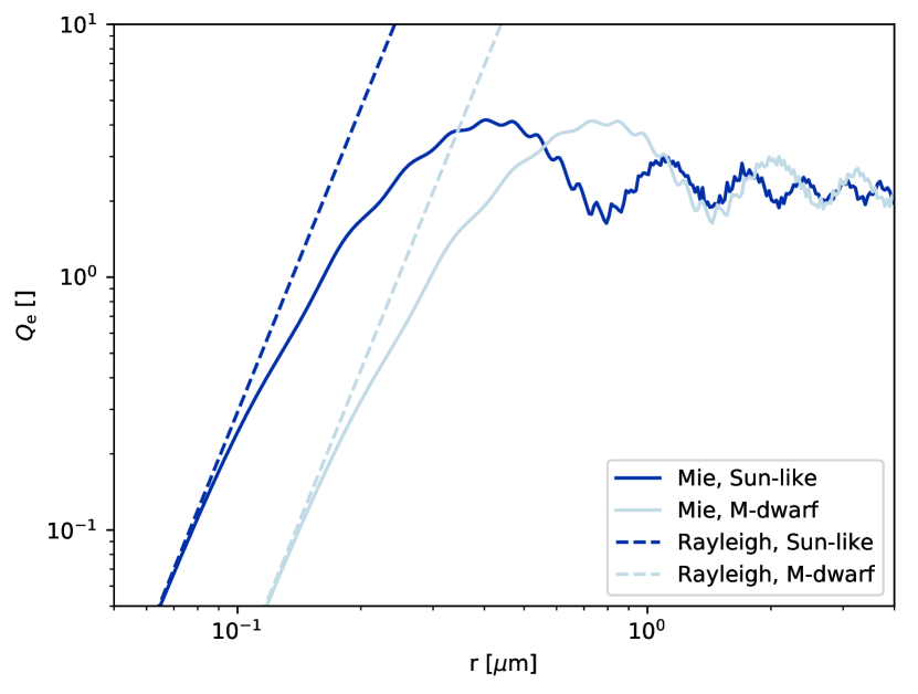
Figure 2: Extinction efficiency ($Q_{\text{e}}$) of H2SO4-H2O aerosols versus average particle radius ($r$). Solid lines are calculated from Mie theory and dashed lines show the Rayleigh limit (valid approximation for small particles). Values for a Sun-like star are in dark blue and those for an M dwarf in light blue.

$Q_{\text{e}}$ is calculated with Mie theory from $r$, the composition of the particle (within the H2SO4-H2O system, specified by $w$), the index of refraction of this given H2SO4-H2O mixture (Palmer and Williams,, 1975), and the wavelength of incident light ($\lambda$) being attenuated (Bohren and Huffman,, 2008). We take $\lambda$ to be the peak of the planet’s host star’s spectrum, which is easily calculated from Wien’s displacement law given the star’s observed effective temperature. Figure 2 shows $Q_{\text{e}}$ as a function of $r$ for both Sun-like ($\lambda=0.556\ \mu$m) and M-dwarf stars (for illustrative purposes, $\lambda=1\ \mu$m) with the Rayleigh limit superimposed. Based on this calculation, we set $r^{\ell}$ = 0.1 $\mu$m for a Sun-like star and $r^{\ell}$ = 0.2 $\mu$m for an M dwarf.

We calculate the aerosol layer vertical path optical depth $\delta$ as

$$\delta=u\kappa_{\text{e}}$$ (4)

where $u$ is the mass column of aerosol particles. We estimate the critical minimum optical depth value for an observable haze layer $\delta^{\ast}$ by simulating transmission spectra. This procedure is described in Section 3.6 after we finish outlining the structure of the rest of the atmosphere.

From the definition of mass column $u$, we can calculate the critical mass of H2SO4 $M^{\ast}_{\ce{H2SO4}}$ as

$$M^{\ast}_{\ce{H2SO4}}=u^{\ast}w4\pi R_{\text{P}}^{2}$$ (5)

where $R_{\text{P}}$ is the radius of the planet. Putting $u^{\ast}$ in terms of $\delta^{\ast}$ and aerosol parameters with Equations (3) and (4), we then calculate the critical number of H2SO4 molecules in aerosols needed to create an observable haze layer as

$$N^{\ast}_{\ce{H2SO4}}=\frac{M^{\ast}_{\ce{H2SO4}}}{m_{\ce{H2SO4}}}=\frac{16\pi}{3}\frac{\delta^{\ast}}{Q_{\text{e}}}r\rho_{\text{aero}}R_{\text{P}}^{2}\frac{w}{m_{\ce{H2SO4}}}$$ (6)

where $m_{\ce{H2SO4}}$ is the mass of a molecule of H2SO4.

3.3 Aerosol Sedimentation and Mixing

Once in the troposphere, H2SO4-H2O aerosols are ideal cloud condensation nuclei because of their high affinity for water, and they are rapidly removed by precipitation (Seinfeld and Pandis,, 2012). For a mean residence time $\tau_{\text{life}}$, H2SO4 remains in the stratosphere as an aerosol contributing to the optical depth of the sulfur haze. We only consider H2SO4 as radiatively relevant until it is transported to the tropopause—the boundary between the isothermal stratosphere and convecting troposphere—because of H2SO4’s short lifetime in the troposphere.

The parameter $\tau_{\text{life}}$ depends on the size of the aerosol. If coagulation and condensation are effective and particles grow large enough, they will gravitationally settle out of the upper atmosphere. Otherwise, small particles will instead likely be removed by dynamic processes first due to their slow settling velocities. Thus, the average lifetime of an H2SO4-H2O aerosol in the stratosphere is approximately

$$\tau_{\text{life}}=\min\{\tau_{\text{fall}},\tau_{\text{mix}}\}$$ (7)

where $\tau_{\text{fall}}$ is the gravitational settling timescale and $\tau_{\text{mix}}$ is the dynamic mixing timescale of exchange between the stratosphere and troposphere.

We calculate $\tau_{\text{fall}}$ from the Stokes velocity of the falling particle as

$$\tau_{\text{fall}}=\frac{z_{\text{fall}}}{v_{\text{Stokes}}}=\frac{9}{2}\frac{z_{\text{fall}}\eta}{r^{2}g\rho_{\text{aero}}C_{\text{C}}}.$$ (8)

Here, $g$ is planet surface gravity, $\eta$ is the dynamic viscosity of air, and $C_{\text{C}}$ is the Cunningham-Stokes correction factor for drag on small particles (Seinfeld and Pandis,, 2012). $z_{\text{fall}}$ is the average distance a sulfur aerosol must fall from its formation location to the tropopause. We conservatively estimate this parameter as the scale height of the stratosphere (i.e., $z_{\text{fall}}=RT_{\text{strat}}(\mu_{\text{air}}g)^{-1}$).

Calculating $\tau_{\text{mix}}$ from first principles is not possible because a general theory of stratosphere-troposphere mixing timescales as a function of external parameters does not yet exist. However, insights can be gained from studying Earth. Today, Earth’s strong stratospheric temperature inversion inhibits this stratosphere-troposphere exchange. Since radiatively generating an upper atmospheric temperature inversion stronger than Earth’s is difficult, Earth’s $\tau_{\text{mix}}$ is likely near an upper bound on stratosphere-troposphere mixing timescales. On the most observable M-dwarf planets, permanent day-night sides of planets due to tidal effects are predicated to generate strong winds (e.g., Showman et al.,, 2010; Showman and Polvani,, 2011) that will almost certainly reduce $\tau_{\text{mix}}$ from Earth values. Therefore, from Earth-based timescales, we estimate $\tau_{\text{mix}}$ = 1 year for all cases (Warneck,, 1999).

3.4 Aerosol Formation

The saturation vapor pressure of H2SO4 at expected terrestrial planet stratosphere temperatures is extremely low ($\ll 10^{-6}$ Pa) (Kulmala and Laaksonen,, 1990), so all stratospheric H2SO4 is effectively found condensed in aerosols rather than as a gas. The sulfur source for H2SO4-H2O aerosols in oxidized atmospheres is SO2 gas. Here, we define $\tau_{\ce{SO2}\rightarrow\ce{H2SO4}}$ as the timescale required to convert stratospheric SO2 to H2SO4. $\tau_{\ce{SO2}\rightarrow\ce{H2SO4}}$ is challenging to calculate precisely because SO2 is oxidized to H2SO4 through a series of photochemical reactions that are poorly constrained both in terms of reaction pathways and rates (Turco et al.,, 1979; Stockwell and Calvert,, 1983; Yung and DeMore,, 1998; Burkholder et al.,, 2015, etc.). The two main stages of the conversion of SO2 to H2SO4 are (1) SO2 is converted to SO3 via a photochemical product and (2) SO3 and H2O react to form H2SO4 (Burkholder et al.,, 2015). For part 1 of the conversion, commonly proposed reactions are

$$\ce{SO2+O+M->SO3+M}$$ (9)

(Yung and DeMore,, 1998; Burkholder et al.,, 2015) or

$$\ce{SO2+OH+M->HSO3+M}$$ (10)

(Turco et al.,, 1979; Stockwell and Calvert,, 1983; Burkholder et al.,, 2015) followed by either

(Turco et al.,, 1979; Stockwell and Calvert,, 1983; Burkholder et al.,, 2015). For part 2, the proposed reaction is

$$\ce{SO3+H2O->H2SO4},$$ (11)

but it is unclear whether this reaction proceeds as a two-body or three-body reaction kinetically (Seinfeld and Pandis,, 2012; Burkholder et al.,, 2015). Large uncertainties in reaction rates for these reactions are compounded by the reaction kinetics’ sensitivity to photochemical product (OH, O) concentrations, which require detailed knowledge of atmospheric composition for accurate results (Jacob,, 1999).

Despite these uncertainties, we can make simplifications because SO2, H2O, and stellar UV photons are essential for the conversion, regardless of the pathway. In particular, because photochemistry is the rate limiting step except potentially in extremely dry atmospheres, we can estimate a lower limit of $\tau_{\ce{SO2}\rightarrow\ce{H2SO4}}$ by considering how long it takes for the number of UV photons necessary for the reaction to proceed to strike the planet’s atmosphere.

For photolysis-driven reactions, the lifetime $\tau$ of the photolyzed species can be described by

$$\tau^{-1}=\frac{1}{4}\int\limits_{\lambda_{\text{UV}}}q(\lambda)\sigma(\lambda)\phi_{\gamma}(\lambda)\mathrm{d}\lambda$$ (12)

where $\lambda$ is wavelength of light, $q$ is the quantum yield or the probability that a photon will dissociate a molecule, $\sigma$ is the absorption cross section of the molecule, $\phi_{\gamma}$ is the flux of photons to a planet’s atmosphere per unit wavelength, and the factor of $\nicefrac{{1}}{{4}}$ accounts for day–night and stellar zenith angle averaging (Jacob,, 1999; Cronin,, 2014). To represent the most rapid conversion rate of SO2 to H2SO4, we set $q=1$ for all wavelengths (i.e., 100% probability that a photon will dissociate a molecule it strikes). At minimum, the SO2 to H2SO4 reaction requires one O or OH molecule. For weakly to strongly oxidized terrestrial planet atmospheres, this photochemical product will most likely be the result of the dissociation of H2O, O2, or CO2. (Ostensibly, photodissociated SO2 could also provide O, but at the surface number densities of SO2 we consider here, SO2 is so optically thin that it cannot effectively absorb photons (Manatt and Lane,, 1993; Hamdy et al.,, 1991).) At each $\lambda$, we set $\sigma(\lambda)$ as the maximum absorption cross section from these three molecules, using data given in Chan et al., (1993), Mota et al., (2005), Lu et al., (2010), Yoshino et al., (1988), Kockarts, (1976), Brion et al., (1979), and Huestis and Berkowitz, (2010).

To set the wavelength for the upper limit of integration, we take the smallest minimum bond dissociation energy of H2O, O2, and CO2 and convert it to a wavelength (via $E_{\text{dis}}=E_{\gamma}=h\nu=hc/\lambda$). A minimum energy of $8.2\times 10^{-19}$ J (deB. Darwent,, 1970) yields a maximum wavelength of 240 nm. We begin the integration from $\lambda=0$ nm for a maximum number of photons. In general, $\phi_{\gamma}$ will be determined from the host star’s spectrum and the distance of the planet from its host star. Here, we use the present-day flux of the Sun to Earth as measured by Thuillier et al., (2004) as a baseline $\phi_{\gamma}$ for a Sun-like star. The ratio of UV flux to stellar bolometric flux declines as stellar mass declines (due to lower effective temperatures and thus higher wavelength Planck peaks) while the ratio of extreme UV (EUV) flux to bolometric flux tends to increase for M dwarfs relative to Sun-like stars due to higher magnetic activity (Scalo et al.,, 2007; Shkolnik and Barman,, 2014; Schaefer et al.,, 2016; Wordsworth et al.,, 2018). The precise change in UV and EUV flux relative to bolometric flux for an M dwarf relative to the Sun will depend on the specific star and its age, but for illustrative purposes here, we assume a $10\times$ decrease in UV flux and a $10\times$ increase in EUV flux relative to the solar value. (Here, we define the EUV wavelength cutoff as $\lambda=91$ nm, following Wordsworth et al., (2018).) Plugging in values to Equation (12) then leads to $\tau_{\ce{SO2}\rightarrow\ce{H2SO4}}^{\ell}\approx$ 3.4 days for a Sun-like star and $\tau_{\ce{SO2}\rightarrow\ce{H2SO4}}^{\ell}\approx$ 2.5 days for an M dwarf. On modern Earth, $\tau_{\ce{SO2}\rightarrow\ce{H2SO4}}\approx 30$ days (Turco et al.,, 1979; Macdonald and Wordsworth,, 2017), which we take as $\tau_{\ce{SO2}\rightarrow\ce{H2SO4}}^{\text{b}}$.

Once we have estimated the lifetimes of H2SO4 and SO2 in the stratosphere, we can directly relate the steady-state $N_{\ce{H2SO4}}$ in aerosols to $N_{\ce{SO2}}$ in gas by assuming that the production rate of H2SO4 is equal to its removal rate:

$$\frac{N_{\ce{H2SO4}}}{\tau_{\text{life}}}=\frac{N_{\ce{SO2}}}{\tau_{\ce{SO2}\rightarrow\ce{H2SO4}}}.$$ (13)

From Equation (13) and the definition of pressure as force over area, $N_{\ce{SO2}}^{\ast}$ converted to a critical partial pressure of SO2 ($p_{\ce{SO2}}^{\ast}$) at the tropopause is

$$p_{\ce{SO2},\text{tropopause}}^{\ast}=N^{\ast}_{\ce{H2SO4}}\frac{gm_{\ce{SO2}}}{4\pi R_{\text{P}}^{2}}\frac{\tau_{\ce{SO2}\rightarrow\ce{H2SO4}}}{\tau_{\text{life}}}$$ (14)

where $m_{\ce{SO2}}$ is the mass of a molecule of SO2.

3.5 Lower Atmosphere Transport

On a wet, temperate planet, SO2 faces no significant sinks below the photochemically active upper atmosphere until it encounters the water cloud layer in the troposphere. Once SO2 encounters condensed water (as either rain or cloud droplets), the SO2 dissolves and is subsequently rained out of the atmosphere (Giorgi and Chameides,, 1985; Seinfeld and Pandis,, 2012; Hu et al.,, 2013). The high effective solubility of SO2 means that effectively all SO2 at and below the cloud deck is removed every rainfall event (Giorgi and Chameides,, 1985). This process of wet deposition greatly limits the lifetime of SO2 in the lower atmosphere and decreases the mixing ratio of SO2 ($f_{\ce{SO2}}\equiv p_{\ce{SO2}}/p$) beyond the water cloud layer in the upper atmosphere relative to the surface.

In our model, we take the mixing ratio of SO2 at the tropopause to be directly proportional to the mixing ratio of SO2 at the surface, such that

$$\frac{p_{\ce{SO2},\text{tropopause}}}{p_{\text{tropopause}}}=\alpha\frac{p_{\ce{SO2},\text{surf}}}{p_{\text{surf}}}.$$ (15)

Here, $p$ is the total atmospheric pressure, and $\alpha$ is the change of mixing ratio between the surface and the upper atmosphere due to the effects of wet deposition. We do not yet know much about hydrological cycles on planets with less surface liquid water than Earth, so in the limiting case we completely ignore wet deposition and set $\alpha^{\ell}$ = 1. For the reasonable case, we assume $\alpha^{\text{b}}$ = 0.1, based on comparison with SO2 vertical profiles measured on Earth (Georgii,, 1978; Meixner,, 1984).

We calculate a pressure-temperature profile from surface temperature $T_{\text{surf}}$ and pressure $p_{\text{surf}}$ assuming a dry adiabat until water vapor becomes saturated and then a moist adiabat until a specified (isothermal) stratospheric temperature $T_{\text{strat}}$ is reached, following the derivation of Wordsworth and Pierrehumbert, (2013). This calculation requires an assumed mixing ratio of water $f_{\ce{H2O}}\equiv p_{\ce{H2O}}/p$ at the surface. This mixing ratio is calculated from relative humidity at the surface $\text{RH}_{\text{surf}}$ and $T_{\text{surf}}$ via $f_{\ce{H2O}\text{,surf}}=\text{RH}_{\text{surf}}\times p_{\text{sat,\ce{H2O}}}(T_{\text{surf}})$ where $p_{\text{sat,\ce{H2O}}}(T_{\text{surf}})$ is the saturation pressure of water at temperature $T_{\text{surf}}$. We set $\text{RH}_{\text{surf}}^{\text{b}}$ = 0.77 like the Earth. Increasing $f_{\ce{H2O}}$ yields a higher tropopause, which results in a higher $p_{\ce{SO2},\text{surf}}$ for a given $p_{\ce{SO2},\text{tropopause}}$. Therefore, we set $\text{RH}_{\text{surf}}^{\ell}$ = 0 (yielding a dry adiabat atmospheric structure).

3.6 Aerosol Observability

Having reviewed the atmospheric conditions dictated by the presence of an observable H2SO4-H2O haze layer, we can now return to the problem of how to calculate the critical optical depth $\delta^{\ast}$ for observation. We simulate the transmission spectra expected of a planet with a sulfur haze for a range of optical depths to determine at which $\delta$-value the hazy spectrum becomes distinct from the clear spectrum. The appendices of Morley et al., (2015, 2017) provide the details of our model for simulating transmission spectra, which uses the matrix prescription presented in Robinson, (2017). We calculate molecular cross sections as described in Freedman et al., (2008, 2014), including an updated water line list from Polyansky et al., (2018).

As inputs to our model, we require aerosol size and number densities, atmospheric gases number densities, and temperature as functions of pressure. From Equation (13), we calculate an H2SO4-H2O aerosol number density profile, assuming exponential decay in aerosols from the tropopause until a parameterized cutoff height (due to lack of photochemical H2SO4 production). We input atmospheric number densities assuming constant mixing ratios (except for H2O) for a given atmospheric composition. The temperature-pressure profile follows a moist adiabat until it reaches an isothermal stratosphere. The mixing ratio of H2O $f_{\ce{H2O}}$ is determined by the moist adiabat. $f_{\ce{H2O}}$ is set at the surface and is held constant until water vapor becomes saturated. Then, $f_{\ce{H2O}}$ evolves according to water’s saturation pressure until the tropopause, above which $f_{\ce{H2O}}$ remains constant.

Varying $\delta$ in these simulated transit spectra for an Earth-like atmosphere (see Section LABEL:subsec:res_obs_haze and Figure LABEL:fig:spectra) suggested that the critical minimum value for an observable haze layer is $\delta^{\ast}\approx 0.1$. Different atmospheres will yield different $\delta^{\ast}$ values, but likely not by orders of magnitude. The precise shape of a hazy planet’s transit spectrum is also somewhat sensitive to the photochemical haze cutoff height. Lower cutoff heights yield more traditionally haze-characteristic flat spectra (e.g., Kreidberg et al.,, 2014), and higher, less physical cutoff heights yield more structured—though still smoothed relative to a clear atmosphere—spectra; but the full range of possible haze cutoff values still yields spectra identifiable as hazy. In the absence of a detailed photochemical model, we choose to display results in Figure LABEL:fig:spectra with a cutoff height of two stratospheric scale heights (11.7 km), following Earth and Venus H2SO4-H2O aerosol profile observations (e.g., Sekiya et al.,, 2016; Knollenberg and Hunten,, 1980).

3.7 Ocean Sulfur Storage

When surface liquid water is present, convection and the hydrological cycle act to bring the lower atmospheric and dissolved sulfur in the ocean into equilibrium rapidly. The partial pressure of SO2 at the surface ($p_{\ce{SO2},\text{surf}}$) is held in equilibrium with the concentration of dissolved, aqueous SO2 in the ocean [SO2 (aq)] via Henry’s law:

$$p_{\ce{SO2},\text{surf}}=K_{\text{H}}(T)[\ce{\ce{SO2}(aq)}],$$ (16)

where $K_{H}=6.96\times 10^{4}$ Pa L mol^-1 is the Henry’s law constant for SO2 (Pierrehumbert,, 2010). Once dissolved, SO2 reacts with the ambient water to form sulfurous acid, which dissociates to H+, HSO3-, and SO3^2- ions:

4.3 Sulfur in the Atmosphere versus Ocean

We next translated our observable sulfur criteria into a critical amount of sulfur in the ocean-atmosphere system. We calculated the distribution of sulfur in an ocean between aqueous S(IV) species (SO2(aq), HSO3-, SO3^2-) as a function of pH, assuming S(IV) saturation, in Figure 5. The fraction of S(IV) stored as SO2—the only dissolved S(IV) species in direct equilibrium with the atmosphere via Equation (16)—exponentially declines as pH increases. For a modern-Earth ocean pH = 8.14, $5.3\times 10^{-6}$% of dissolved S(IV) is SO2(aq), 10.3% is HSO3-, and 89.7% is SO3^2-.

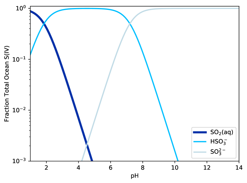
Figure 5: Distribution of aqueous S(IV) species SO2(aq) (dark blue), HSO3- (medium blue), and SO3^2- (light blue) as a function of pH from the reactions (LABEL:eq:aq_react1)-(LABEL:eq:aq_react2). Only SO2(aq) is directly in equilibrium with the atmosphere.

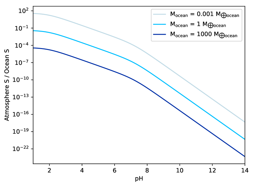
Figure 6: The ratio of S in SO2 in the atmosphere compared to S in S(IV) in the ocean from $N_{\ce{S(IV)}\text{,oc}}$ and $N_{\ce{S}\text{,atm}}$ given in Equations (LABEL:eq:S_crit_ocean) and (LABEL:eq:S_atm_crit_so2), respectively, versus ocean pH.

From the distribution of S(IV) species, we then calculated the expected ratio of S(IV) sulfur in the atmosphere (SO2) to S(IV) sulfur in the ocean (SO2(aq), HSO3-, SO3^2-), again assuming saturation of aqueous S(IV) and atmosphere-ocean equilibrium. Figure 6 shows the preferential storage of S(IV) in the ocean over the atmosphere as a function of pH with varying total ocean mass. The storage capacity of the ocean linearly increases with increasing ocean mass and exponentially increases with increasing ocean pH. For Earth ocean pH and mass, the ratio of atmospheric to oceanic S(IV) is $2.13\times 10^{-9}$. (Note that this ratio is not actually observed in the modern ocean as the assumption of S(IV) saturation is violated because of the instability of aqueous S(IV).)

4.4 Observable Sulfur versus Ocean Parameters

Finally, we look at how the presence and characteristics of an ocean shape sulfur observability. First, we calculated conditions for atmospheric sulfur observability for a range of ocean pHs and masses using the best-guess model parameters given in Table LABEL:tab:parameters. Then, we calculated these conditions using the limiting parameters. For all inputs, we plot contours of the critical timescale for S(IV) decay ($\tau_{\ce{S(IV)}}^{\ast}$) necessary to have enough sulfur in the atmosphere-ocean system to sustain observable SO2 or an observable H2SO4-H2O aerosol layer versus ocean parameters of pH and mass. From present aqueous redox sulfur chemistry experimental results, we set $\tau_{\ce{S(IV)}}^{\ast}=0.1$ years $\approx 1$ month (white contour) as a reasonable timescale for aqueous S(IV) decay. For ocean pHs and total masses below this line, observable atmospheric sulfur is possible. Above this line, observable sulfur grows increasingly unlikely.

Low pH is most favorable for observable atmospheric sulfur in our results, but cations from surface weathering can act to buffer pH and likely maintain a pH near neutral (Grotzinger and Kasting,, 1993), particularly in low water content regimes with lots of exposed land. Empirically, paleo-pH estimates for both Earth and Mars seem to favor such a near-neutral regime (e.g., Halevy,, 2013; Grotzinger et al.,, 2014). From these considerations, we choose pH = 6 to report characteristic ocean sizes leading to observable atmospheric sulfur, given $\tau_{\ce{S(IV)}}^{\ast}=0.1$ years. We also choose, somewhat arbitrarily, to define significant surface liquid water as $10^{-3}$ Earth ocean masses or a global equivalent ocean layer of 2.75 m on an Earth-sized planet. For context, on Earth today, this amount of water is equivalent to about one third of the Mediterranean Sea (Eakins and Sharman,, 2010).

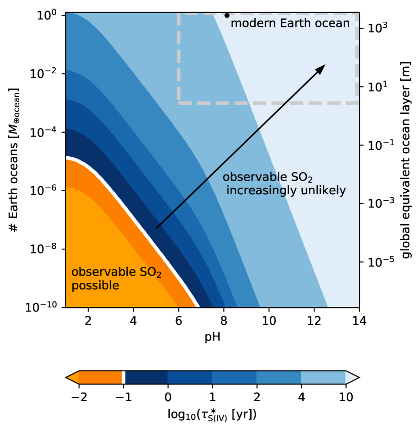
Figure 7: Contours of the critical lifetime of aqueous S(IV) (sulfur in redox state +4, in equilibrium with atmosphere) $\tau_{\ce{S(IV)}^{\ast}}$ for observable mixing ratios of SO2 versus ocean pH and mass (in Earth ocean masses). Model results are shown for the best-guess model parameters described in the text. The white contour indicates a reasonable timescale for aqueous S(IV) decay. The dashed gray lines indicate ocean parameters of interest (from a reasonable pH limit of 6 and a low-liquid-water threshold of 0.001 $M_{\oplus\text{ocean}}$).

Figure 7 shows $\tau_{\ce{S(IV)}}^{\ast}$ versus ocean parameters for observing SO2 with our best-guess parameter values. For surface liquid water content greater than $10^{-3}$ Earth ocean masses, observable SO2 with reasonable model parameters requires $\tau_{\ce{S(IV)}}^{\ast}\gtrsim$ 10 years for even the lowest pHs most favorable for SO2 buildup and $\tau_{\ce{S(IV)}}^{\ast}>$ 10,000 years for pH $>6$. Such long decay times are incompatible with present highest quoted values for decay in the literature, which are on the order of years (Ranjan et al.,, 2018). At pH = 6 and $\tau_{\ce{S(IV)}}^{\ast}=0.1$ years, observable SO2 requires an “ocean” of less than $1\times 10^{-9}$ Earth’s ocean mass or a global equivalent layer of less than 3 $\mu$m.

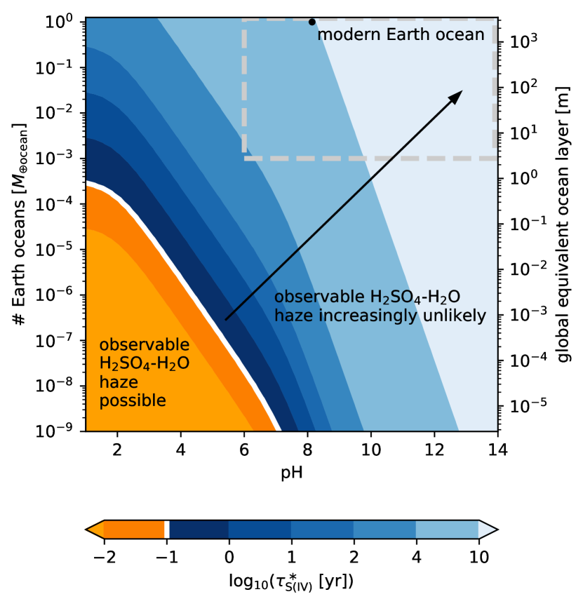
Figure 8: Contours of the critical lifetime of aqueous S(IV) $\tau_{\ce{S(IV)}^{\ast}}$ for the formation of an observable H2SO4-H2O haze layer versus ocean pH and mass (in Earth oceans). Model results are shown for the best-guess model parameters described in the text.

Figure 8 shows $\tau_{\ce{S(IV)}}^{\ast}$ versus ocean parameters for observing an H2SO4-H2O haze layer with our best guess parameter values. For surface liquid water content greater than $10^{-3}$ Earth ocean masses, observable haze formation with reasonable model parameters requires $\tau_{\ce{S(IV)}}^{\ast}\gtrsim$ 1 year for all pHs and, again, $\tau_{\ce{S(IV)}}^{\ast}>$10,000 years for pH$>6$. Again, these timescales are much, much longer than any $\tau_{\ce{S(IV)}}^{\ast}$ estimates currently present in the literature. At pH = 6 and $\tau_{\ce{S(IV)}}^{\ast}=0.1$ years, observable haze requires an ocean of less than $2.5\times 10^{-8}$ Earth’s ocean mass or a global equivalent layer of less than 68 $\mu$m.

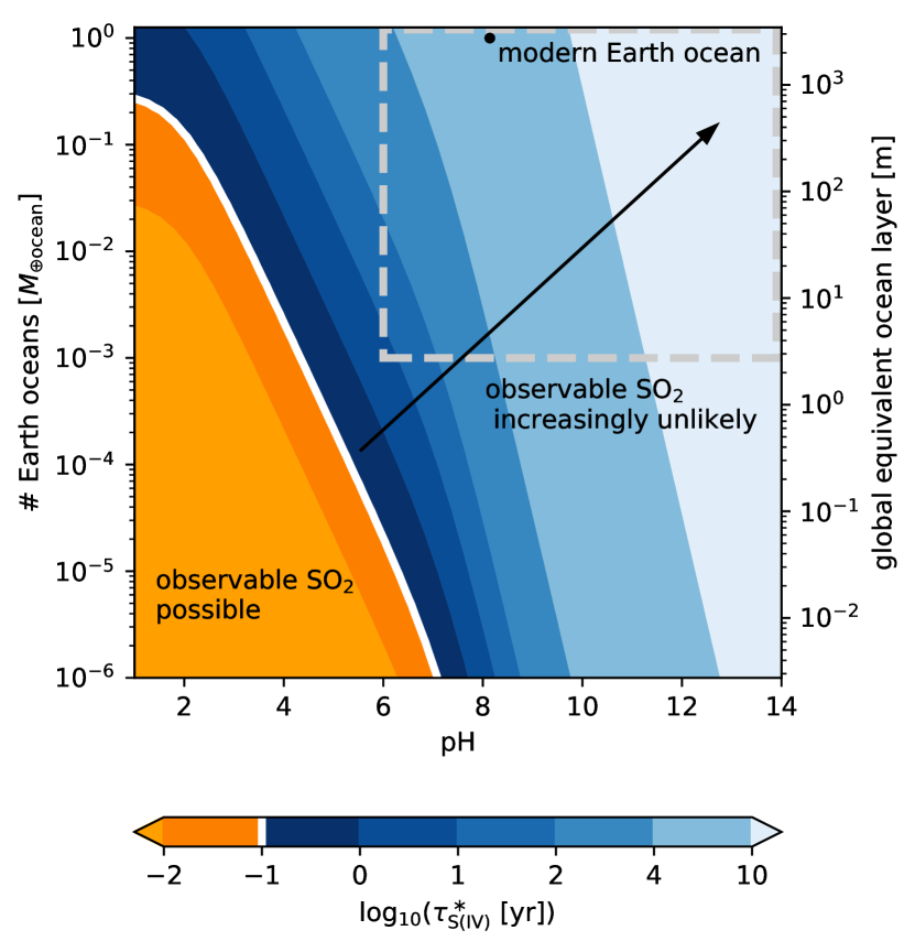
Figure 9: Contours of the critical lifetime of aqueous S(IV) $\tau_{\ce{S(IV)}^{\ast}}$ for the formation of an observable H2SO4-H2O haze layer versus ocean pH and mass (in Earth oceans). Model results are shown for the limiting set of model parameters described in the text.

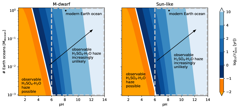
Figure 10: Contours of the critical lifetime of aqueous S(IV) $\tau_{\ce{S(IV)}^{\ast}}$ for the formation of an observable H2SO4-H2O haze layer versus ocean pH and mass (in Earth oceans) for a planet around an M dwarf (left) and Sun-like star (right). Model results are shown for the limiting set of model parameters described in the text.

Figures 9 and 10 show $\tau_{\ce{S(IV)}}^{\ast}$ versus ocean parameters for observing SO2 and observing a haze layer, respectively, with our limiting parameter values. At pH = 6 and $\tau_{\ce{S(IV)}}^{\ast}=0.1$ years, observable SO2 with these most stringent parameters still requires an ocean of less than $2\times 10^{-5}$ Earth’s ocean mass or a global equivalent layer less than 5.5 cm. We calculate that at pH = 6 and $\tau_{\ce{S(IV)}}^{\ast}=0.1$ years, an observable haze layer for a planet around an M-dwarf star requires an ocean of less than $1.3\times 10^{-3}$ Earth’s ocean mass or a global equivalent layer of 3.6 m; around a Sun-like star gives an ocean of less than $1.5\times 10^{-3}$ Earth’s ocean mass or a global equivalent layer of 4.1 m.

5 Discussion

5.1 Model Uncertainties

Robustly establishing sustained high trace mixing ratios of SO2 and H2SO4-H2O haze as indicators of limited surface liquid water will require experimental constraints on S(IV) decay pathways and kinetics. Better theoretical constraints on the upper bounds of sulfur outgassing rates and lower bounds of ocean pHs in water-limited regimes will also improve the robustness of these newly proposed observational constraints on surface liquid water.

However, in accounting for these poorly constrained inputs, we have concocted a worst-case scenario for each input, often physically inconsistent with each other (e.g., extremely high sulfur outgassing levels would not be consistent with extremely small aerosol particles microphysically). These limiting parameters are intended to push our model to its limits given the breadth of our unknown parameters, rather than just presenting likely values informed by predominantly Earth-based Solar System information. The incompatibility of observable SO2 to below our threshold of significant liquid water by almost two orders of magnitude and the incompatibility of observable H2SO4-H2O aerosols to very near our threshold of significant liquid water for these limiting conditions place the extremely strong constraints on surface liquid water for our best-guess model parameters into a larger context. Further, many of these model parameters will be more constrainable for individual systems with observations. Stellar spectrum observations would help constrain the timescale of SO2 to H2SO4 conversion $\tau_{\ce{SO2}\rightarrow\ce{H2SO4}}$, and observable stellar properties like rotation rate would help constrain stellar age, which would help place limits on the evolution of outgassing flux $\dot{N_{\ce{S}}}$.

Though in this paper we have emphasized the benefits of using a simple model for our immediate hypothesis test, in the future a hierarchy of models of varying complexities will be useful. Future work employing more complicated photochemistry, microphysics, aqueous chemistry, and interior dynamics models will allow for more detailed evaluations of the constrainability of surface liquid water from oxidized atmospheric sulfur observations in specific planetary scenarios. Such work would be particularly useful if it were combined with improved experimental constraints on key reaction rates in the atmosphere and ocean.

5.2 Oxidation State of the Atmosphere

Currently, the proposed atmospheric sulfur anti-ocean signatures are limited in scope to oxidized atmospheres. Theoretical predictions of the redox evolution of planets orbiting M dwarfs (our most observable targets) suggest such planets are more likely than those orbiting Sun-like stars to evolve toward more oxidized atmospheric conditions, given M-stars’ extended high EUV and UV flux period for their first gigayear of main sequence life (Shkolnik and Barman,, 2014) and the consequent higher potential for H2O dissociation, H2 escape, and O2 buildup (Luger and Barnes,, 2015; Tian and Ida,, 2015; Wordsworth et al.,, 2018). Depending on planetary age and thermal evolution, this O2 may be simply maintained in the atmosphere, or it may be absorbed into the mantle during a magma ocean phase and influence the oxidation state of the secondary outgassed atmosphere, but either way the planet is driven toward a more oxidized atmosphere (Wordsworth et al.,, 2018). (Planets with Sun-like host stars can also undergo this process, although in this case its effectiveness is likely more dependent on the composition of the planet’s atmosphere (Catling et al.,, 2001; Wordsworth and Pierrehumbert,, 2013, 2014).) We can reasonably expect to encounter the oxidized planets that these methods apply to. Regardless, the study of the compatibility of buildup of sulfur gas and sulfur aerosol formation with liquid water could be extended to reduced atmospheres (featuring H2S gas and S8 aerosols) after better experimental characterization of the photochemical reactions that produce S8 and the removal rates of associated dissolved products of H2S.

Observationally determining the general oxidation state of a planet’s atmosphere will be possible from transit spectra in many cases. H2-dominated atmospheres, which are strongly reducing, are identifiable from their extremely high scale heights due to low average molecular mass. CO2 and CH4 both have strong spectral features and have the potential to be identified even when not dominant atmospheric gases (Lincowski et al.,, 2018). While these carbon-bearing species can coexist to some extent, in terrestrial atmospheres, CO2 is the dominant carbon molecule in oxidized atmospheres and CH4 or CO in reduced atmospheres (Hu et al.,, 2012). Measuring CO2-to-CH4 (or CO) ratios can thus help to constrain an atmosphere’s redox state.

5.3 Identifying Haze as H2SO4-H2O

Identifying haze particles as H2SO4-H2O aerosols is challenging but tractable. While we leave explicit modeling of haze composition retrieval with stellar noise and specific instrument systematics to future work, we discuss the basic logistics of H2SO4-H2O identification here.

H2SO4-H2O aerosols are only weakly absorbing at visible wavelengths, so Mie scattering dominates their spectral effects. They therefore tend to lack distinctively characteristic spectral fingerprints (Hu et al.,, 2013). Our simulated transit spectra tests of aerosol cutoff height sensitivity suggest that if the aerosols were to extend throughout much of the otherwise optically thin upper atmosphere ($\gtrsim$ 5 scale heights), H2SO4-H2O features could become identifiable. Such high extents would seem to be disfavored from H2SO4 photochemical production and SO2 vertical transport considerations, but more detailed photochemical modeling and simulated retrievals are required to determine whether this direct identification possibility is actually feasible. Regardless, H2SO4-H2O aerosols still have distinct radiative and formation properties when compared to other key spectra-flattening candidates: water clouds, organic photochemical hazes, and elemental sulfur hazes.

We tested the ability to distinguish both low-lying water clouds and higher ice clouds (with Earth-like characteristics) from an H2SO4-H2O haze layer, but even at our assumed 100% cloud coverage, the H2SO4-H2O haze is clearly distinguishable from H2O clouds; the transit spectrum is probing higher optical depths than expected lower cloud peak heights, and even the higher ice clouds are too low to significantly flatten the transit spectrum. The latter two alternative spectra-flattening candidates—S8 and photochemical haze—require reducing atmospheres to form. Identification of an atmosphere as oxidizing, as described in the preceding section, strongly disfavors these species’ formation. Distinguishing H2SO4-H2O aerosols from S8 aerosols that form in reduced atmospheres could also be possible from a distinct spectral feature: S8 aerosols’ radiative properties transition sharply between 0.3 $\mu$m and 0.5 $\mu$m from dominantly attenuating light via absorption to scattering (Hu et al.,, 2013); H2SO4-H2O aerosols do not exhibit this feature.

Organic photochemical hazes are an active research topic (e.g., Hörst et al.,, 2018), but many studies suggest that they require CH4/CO2 ratios $\gtrsim$ 0.1 (DeWitt et al.,, 2009). Spectra indicating significant CO2 and the absence of substantial mixing ratios of CH4 would therefore further disfavor organic photochemical haze as the spectra-flattening agent. Additionally, organic photochemical hazes form as fractal aggregates (Bar-Nun et al.,, 1988) while H2SO4-H2O aerosols are spherical (Knollenberg and Hunten,, 1980). These distinct shapes have different radiative properties (Wolf and Toon,, 2010), which also have the potential to be recovered via inverse modeling (Ackerman and Marley,, 2001).

5.4 Life’s Impact on the Sulfur Cycle

We have neglected the influence of life on the sulfur cycle throughout this paper. Of course, constraining liquid water abundance is in the pursuit of finding life beyond Earth, so we would be remiss not to address life’s influence on the sulfur cycle as we have presented it here. The most important direct effect would be sulfur-consuming life’s capacity to exchange redox states of aqueous sulfur not expected from basic redox reactions (Johnston,, 2011; Kharecha et al.,, 2005). The thermodynamic instability of aqueous S(IV) species makes them an attractive microbial food source, so even if S(IV) is the waste product of one organism’s metabolism, it is likely to be rapidly consumed again and converted back to another redox state. The largest concern for our picture is the potential for metabolic chains to produce dissolved H2S species, which will be in equilibrium with atmospheric H2S via Henry’s law, that could be oxidized to SO2 in the atmosphere and thus yield a new, unaccounted source of SO2. However, this process would serve as an effective recycling term of sulfur that would be a fraction of outgassing. As a less than order of magnitude effect, this recycling is not likely to impact the conclusions of our study, and thus we do not expect these proposed liquid water constraining methods to be invalidated by the presence of life. We also neglect the possibility of intelligent life modifying its environment via sulfur products (e.g., Caldeira et al.,, 2013); we leave coupled ecosystem-sulfur cycle studies as an intriguing topic for future investigation.

5.5 Extensions to Observational Techniques beyond Transmission Spectroscopy

Finally, we have focused our efforts in this paper on observations of the sulfur cycle via transmission spectroscopy; however, our analysis could easily be extended to other observational techniques, notably reflected light spectroscopy given our interest in temperate planets. The impact of different observational techniques is in estimating the critical atmospheric sulfur mass that becomes observable. The technique of interest supplies a critical mass path $u^{\ast}$ or a critical aerosol optical depth $\delta^{\ast}$ at which SO2 or H2SO4-H2O aerosols, respectively, become observable. Once this calculation is complete, evaluating the feasibility of atmospheric sulfur buildup for a given amount of surface liquid water will be straightforward using our open-source sulfur model.

6 Conclusion

The presence of liquid water on an oxidized planet strongly influences its sulfur cycle—particularly the planet’s ability to sustain an optically thick H2SO4-H2O haze layer or a high trace mixing ratio of SO2 gas. Detectable levels of both H2SO4-H2O aerosols and SO2 gas require SO2 in the upper atmosphere, but the presence of an ocean restricts the availability of SO2 in the atmosphere. For expected ocean pHs, exponentially more SO2 is stored in the ocean than in the atmosphere because of basic chemical properties of aqueous SO2. Within the ocean, the dissolved products of SO2 are thermodynamically unstable and thus short-lived. Recent outgassing must supply both the SO2 present in the atmosphere necessary for observation and the accompanying amount of aqueous sulfur implied by the size of the ocean.

Via a quantitative model of this wet, oxidized sulfur cycle, we have shown that neither observable H2SO4-H2O haze layers nor observable levels of SO2 are likely compatible with significant surface liquid water ($\gtrsim 10^{-3}$ Earth ocean masses). Despite the uncertainties involved in modeling exoplanet processes, this incompatibility seems to persist even in the most extreme physical conditions to promote SO2 buildup and haze formation. Thus, we propose the observational detection of H2SO4-H2O haze and SO2 gas as two new constraints on surface liquid water.

The code for our sulfur cycle model is available at https://github.com/kaitlyn-loftus/alien-sulfur-cycles. This work was supported by NASA grants 80NSSC18K0829 and NNX16AR86G. KL thanks Matthew Brennan, Junjie Dong, David Johnston, and Itay Halevy for helpful discussions on various aspects of sulfur chemistry. The authors also thank James Kasting for a productive review.

References

- Ackerman and Marley, (2001) Ackerman, A. S. and Marley, M. S. (2001). Precipitating condensation clouds in substellar atmospheres. The Astrophysical Journal, 556(2):872.
- Anderson, (1974) Anderson, A. (1974). Chlorine, sulfur, and water in magmas and oceans. Geological Society of America Bulletin, 85(9):1485–1492.
- Avrahami and Golding, (1968) Avrahami, M. and Golding, R. (1968). The oxidation of the sulphide ion at very low concentrations in aqueous solutions. Journal of the Chemical Society A: Inorganic, Physical, Theoretical, pages 647–651.
- Bar-Nun et al., (1988) Bar-Nun, A., Kleinfeld, I., and Ganor, E. (1988). Shape and optical properties of aerosols formed by photolysis of acetylene, ethylene, and hydrogen cyanide. Journal of Geophysical Research: Atmospheres, 93(D7):8383–8387.
- Bohren and Huffman, (2008) Bohren, C. F. and Huffman, D. R. (2008). Absorption and scattering of light by small particles. John Wiley & Sons.
- Boulegue, (1978) Boulegue, J. (1978). Solubility of elemental sulfur in water at 298 k. Phosphorus and Sulfur and the related Elements, 5(1):127–128.
- Brimblecombe and Lein, (1989) Brimblecombe, P. and Lein, A. Y. (1989). Evolution of the global biogeochemical sulphur cycle. New York, NY; John Wiley and Sons Inc.
- Brion et al., (1979) Brion, C., Tan, K., Van der Wiel, M., and Van der Leeuw, P. E. (1979). Dipole oscillator strengths for the photoabsorption, photoionization and fragmentation of molecular oxygen. Journal of Electron Spectroscopy and Related Phenomena, 17(2):101–119.
- Burkholder et al., (2015) Burkholder, J., Sander, S., Abbatt, J., Barker, J., Huie, R., Kolb, C., Kurylo, M., Orkin, V., Wilmouth, D., and Wine, P. (2015). Chemical kinetics and photochemical data for use in atmospheric studies: evaluation number 18. Technical report, Pasadena, CA: Jet Propulsion Laboratory, National Aeronautics and Space ….
- Caldeira et al., (2013) Caldeira, K., Bala, G., and Cao, L. (2013). The science of geoengineering. Annual Review of Earth and Planetary Sciences, 41(1):231–256.
- Catling et al., (2001) Catling, D. C., Zahnle, K. J., and McKay, C. P. (2001). Biogenic methane, hydrogen escape, and the irreversible oxidation of early earth. Science, 293(5531):839–843.
- Chan et al., (1993) Chan, W., Cooper, G., and Brion, C. (1993). The electronic spectrum of water in the discrete and continuum regions. absolute optical oscillator strengths for photoabsorption (6–200 ev). Chemical physics, 178(1-3):387–400.
- Cowan et al., (2012) Cowan, N. B., Abbot, D. S., and Voigt, A. (2012). A false positive for ocean glint on exoplanets: The latitude-albedo effect. The Astrophysical Journal Letters, 752(1):L3.
- Cowan et al., (2009) Cowan, N. B., Agol, E., Meadows, V. S., Robinson, T., Livengood, T. A., Deming, D., Lisse, C. M., A’Hearn, M. F., Wellnitz, D. D., Seager, S., et al. (2009). Alien maps of an ocean-bearing world. The Astrophysical Journal, 700(2):915.
- Cronin, (2014) Cronin, T. W. (2014). On the choice of average solar zenith angle. Journal of the Atmospheric Sciences, 71(8):2994–3003.
- deB. Darwent, (1970) deB. Darwent, B. (1970). Bond dissociation energies in simple molecules. NSRDS-NBS 31.
- Deming et al., (2013) Deming, D., Wilkins, A., McCullough, P., Burrows, A., Fortney, J. J., Agol, E., Dobbs-Dixon, I., Madhusudhan, N., Crouzet, N., Desert, J.-M., et al. (2013). Infrared transmission spectroscopy of the exoplanets hd 209458b and xo-1b using the wide field camera-3 on the hubble space telescope. The Astrophysical Journal, 774(2):95.
- DeWitt et al., (2009) DeWitt, H. L., Trainer, M. G., Pavlov, A. A., Hasenkopf, C. A., Aiken, A. C., Jimenez, J. L., McKay, C. P., Toon, O. B., and Tolbert, M. A. (2009). Reduction in haze formation rate on prebiotic earth in the presence of hydrogen. Astrobiology, 9(5):447–453.
- Domagal-Goldman et al., (2014) Domagal-Goldman, S. D., Segura, A., Claire, M. W., Robinson, T. D., and Meadows, V. S. (2014). Abiotic ozone and oxygen in atmospheres similar to prebiotic earth. The Astrophysical Journal, 792(2):90.
- Eakins and Sharman, (2010) Eakins, B. and Sharman, G. (2010). Volumes of the world’s oceans from etopo1. NOAA National Geophysical Data Center, Boulder, CO, 7.
- Edmonds and Mather, (2017) Edmonds, M. and Mather, T. A. (2017). Volcanic sulfides and outgassing. Elements, 13(2):105–110.
- Ermakov and Purmal, (2001) Ermakov, A. N. and Purmal, A. P. (2001). Catalytic mechanism of the “noncatalytic” autooxidation of sulfite. Kinetics and catalysis, 42(4):479–489.
- Fortney, (2005) Fortney, J. J. (2005). The effect of condensates on the characterization of transiting planet atmospheres with transmission spectroscopy. Monthly Notices of the Royal Astronomical Society, 364(2):649–653.
- Fraine et al., (2014) Fraine, J., Deming, D., Benneke, B., Knutson, H., Jordán, A., Espinoza, N., Madhusudhan, N., Wilkins, A., and Todorov, K. (2014). Water vapour absorption in the clear atmosphere of a neptune-sized exoplanet. Nature, 513(7519):526.
- Freedman et al., (2014) Freedman, R. S., Lustig-Yaeger, J., Fortney, J. J., Lupu, R. E., Marley, M. S., and Lodders, K. (2014). Gaseous mean opacities for giant planet and ultracool dwarf atmospheres over a range of metallicities and temperatures. The Astrophysical Journal Supplement Series, 214(2):25.
- Freedman et al., (2008) Freedman, R. S., Marley, M. S., and Lodders, K. (2008). Line and mean opacities for ultracool dwarfs and extrasolar planets. The Astrophysical Journal Supplement Series, 174(2):504.
- Georgii, (1978) Georgii, H.-W. (1978). Large scale spatial and temporal distribution of sulfur compounds. In Sulfur in the Atmosphere, pages 681–690. Elsevier.
- Gerlach et al., (1996) Gerlach, T. M., Westrich, H. R., and Symonds, R. B. (1996). Preeruption vapor in magma of the climactic mount pinatubo eruption: Source of the giant stratospheric sulfur dioxide cloud. Fire and mud: eruptions and lahars of Mount Pinatubo, Philippines, 415:33.
- Giorgi and Chameides, (1985) Giorgi, F. and Chameides, W. (1985). The rainout parameterization in a photochemical model. Journal of Geophysical Research: Atmospheres, 90(D5):7872–7880.
- Goldhaber, (2003) Goldhaber, M. (2003). Sulfur-rich sediments. Treatise on Geochemistry, 7:407.
- Grotzinger and Kasting, (1993) Grotzinger, J. P. and Kasting, J. F. (1993). New constraints on precambrian ocean composition. The Journal of Geology, 101(2):235–243.
- Grotzinger et al., (2014) Grotzinger, J. P., Sumner, D. Y., Kah, L., Stack, K., Gupta, S., Edgar, L., Rubin, D., Lewis, K., Schieber, J., Mangold, N., et al. (2014). A habitable fluvio-lacustrine environment at yellowknife bay, gale crater, mars. Science, 343(6169):1242777.
- Guekezian et al., (1997) Guekezian, M., Coichev, N., Suárez-Iha, M. E. V., and Neves, E. d. A. (1997). Stability of sulfur (iv) solutions in the presence of amines and the tendency of sulfite ions to disproportionate in stock solutions. Analytical letters, 30(7):1423–1436.
- Halevy, (2013) Halevy, I. (2013). Production, preservation, and biological processing of mass-independent sulfur isotope fractionation in the archean surface environment. Proceedings of the National Academy of Sciences, 110(44):17644–17649.
- Halevy and Bachan, (2017) Halevy, I. and Bachan, A. (2017). The geologic history of seawater ph. Science, 355(6329):1069–1071.
- Halevy et al., (2007) Halevy, I., Zuber, M. T., and Schrag, D. P. (2007). A Sulfur Dioxide Climate Feedback on Early Mars. Science, 318:1903.
- Halmer et al., (2002) Halmer, M. M., Schmincke, H.-U., and Graf, H.-F. (2002). The annual volcanic gas input into the atmosphere, in particular into the stratosphere: a global data set for the past 100 years. Journal of Volcanology and Geothermal Research, 115(3-4):511–528.
- Hamdy et al., (1991) Hamdy, H., He, Z., and Samson, J. (1991). Precision photoabsorption cross section measurements of so2 from 147 to 1017 a. Journal of Physics B: Atomic, Molecular and Optical Physics, 24(22):4803.
- Hansen and Hovenier, (1974) Hansen, J. E. and Hovenier, J. (1974). Interpretation of the polarization of venus. Journal of the Atmospheric Sciences, 31(4):1137–1160.
- (40) Harman, C., Felton, R., Hu, R., Domagal-Goldman, S. D., Segura, A., Tian, F., and Kasting, J. (2018a). Abiotic o2 levels on planets around f, g, k, and m stars: effects of lightning-produced catalysts in eliminating oxygen false positives. The Astrophysical Journal, 866(1):56.
- (41) Harman, C., Pavlov, A., Babikov, D., and Kasting, J. (2018b). Chain formation as a mechanism for mass-independent fractionation of sulfur isotopes in the archean atmosphere. Earth and Planetary Science Letters, 496:238–247.
- Hayon et al., (1972) Hayon, E., Treinin, A., and Wilf, J. (1972). Electronic spectra, photochemistry, and autoxidation mechanism of the sulfite-bisulfite-pyrosulfite systems. so2-, so3-, so4-, and so5-radicals. Journal of the American Chemical Society, 94(1):47–57.
- Hörst et al., (2018) Hörst, S. M., He, C., Lewis, N. K., Kempton, E. M.-R., Marley, M. S., Morley, C. V., Moses, J. I., Valenti, J. A., and Vuitton, V. (2018). Haze production rates in super-earth and mini-neptune atmosphere experiments. Nature Astronomy, 2(4):303.
- Hu et al., (2012) Hu, R., Seager, S., and Bains, W. (2012). Photochemistry in Terrestrial Exoplanet Atmospheres. I. Photochemistry Model and Benchmark Cases. ApJ, 761:166.
- Hu et al., (2013) Hu, R., Seager, S., and Bains, W. (2013). Photochemistry in Terrestrial Exoplanet Atmospheres. II. H2S and SO2 Photochemistry in Anoxic Atmospheres. ApJ, 769:6.
- Huestis and Berkowitz, (2010) Huestis, D. L. and Berkowitz, J. (2010). Critical evaluation of the photoabsorption cross section of co2 from 0.125 to 201.6 nm at room temperature. In Bulletin of the American Astronomical Society, volume 42, page 972.
- Huitson et al., (2013) Huitson, C. M., Sing, D. K., Pont, F., Fortney, J., Burrows, A., Wilson, P. A., Ballester, G., Nikolov, N., Gibson, N., Deming, D., et al. (2013). An hst optical-to-near-ir transmission spectrum of the hot jupiter wasp-19b: detection of atmospheric water and likely absence of tio. Monthly Notices of the Royal Astronomical Society, 434(4):3252–3274.
- Jacob, (1999) Jacob, D. (1999). Introduction to atmospheric chemistry. Princeton University Press.
- Jacobson et al., (2000) Jacobson, M., Charlson, R. J., Rodhe, H., and Orians, G. H. (2000). Earth System Science: from biogeochemical cycles to global changes, volume 72. Academic Press.
- Johnston, (2011) Johnston, D. T. (2011). Multiple sulfur isotopes and the evolution of Earth’s surface sulfur cycle. Earth Science Reviews, 106:161–183.
- Jugo, (2009) Jugo, P. J. (2009). Sulfur content at sulfide saturation in oxidized magmas. Geology, 37(5):415–418.
- Jugo et al., (2005) Jugo, P. J., Luth, R. W., and Richards, J. P. (2005). An experimental study of the sulfur content in basaltic melts saturated with immiscible sulfide or sulfate liquids at 1300° c and 1· 0 gpa. Journal of Petrology, 46(4):783–798.
- Kaltenegger et al., (2010) Kaltenegger, L., Henning, W. G., and Sasselov, D. D. (2010). Detecting Volcanism on Extrasolar Planets. AJ, 140:1370–1380.
- Kaltenegger and Sasselov, (2010) Kaltenegger, L. and Sasselov, D. (2010). Detecting planetary geochemical cycles on exoplanets: atmospheric signatures and the case of so2. The Astrophysical Journal, 708(2):1162–1167.
- Karchmer, (1970) Karchmer, J. H., editor (1970). Analytical chemistry of sulfur and its compounds. Wiley-Interscience.
- Kasting, (2012) Kasting, J. (2012). How to find a habitable planet. Princeton University Press.
- Kasting et al., (1993) Kasting, J. F., Whitmire, D. P., and Reynolds, R. T. (1993). Habitable zones around main sequence stars. Icarus, 101(1):108–128.
- Kasting et al., (1989) Kasting, J. F., Zahnle, K. J., Pinto, J. P., and Young, A. T. (1989). Sulfur, ultraviolet radiation, and the early evolution of life. Origins of Life and Evolution of the Biosphere, 19:95–108.
- Kempe and Degens, (1985) Kempe, S. and Degens, E. T. (1985). An early soda ocean? Chemical Geology, 53(1-2):95–108.
- Kharecha et al., (2005) Kharecha, P., Kasting, J., and Siefert, J. (2005). A coupled atmosphere–ecosystem model of the early archean earth. Geobiology, 3(2):53–76.
- Kite et al., (2009) Kite, E. S., Manga, M., and Gaidos, E. (2009). Geodynamics and rate of volcanism on massive earth-like planets. The Astrophysical Journal, 700(2):1732.
- Knollenberg and Hunten, (1980) Knollenberg, R. and Hunten, D. (1980). The microphysics of the clouds of venus: Results of the pioneer venus particle size spectrometer experiment. Journal of Geophysical Research: Space Physics, 85(A13):8039–8058.
- Kockarts, (1976) Kockarts, G. (1976). Absorption and photodissociation in the schumann-runge bands of molecular oxygen in the terrestrial atmosphere. Planetary and Space Science, 24(6):589–604.
- Kopparapu et al., (2013) Kopparapu, R. K., Ramirez, R., Kasting, J. F., Eymet, V., Robinson, T. D., Mahadevan, S., Terrien, R. C., Domagal-Goldman, S., Meadows, V., and Deshpande, R. (2013). Habitable zones around main-sequence stars: new estimates. The Astrophysical Journal, 765(2):131.
- Kreidberg et al., (2014) Kreidberg, L., Bean, J. L., Désert, J.-M., Benneke, B., Deming, D., Stevenson, K. B., Seager, S., Berta-Thompson, Z., Seifahrt, A., and Homeier, D. (2014). Clouds in the atmosphere of the super-Earth exoplanet GJ1214b. Nature, 505:69–72.
- Kulmala and Laaksonen, (1990) Kulmala, M. and Laaksonen, A. (1990). Binary nucleation of water-sulfuric acid system: Comparison of classical theories with different H2SO4 saturation vapor pressures. J. Chem. Phys., 93:696–701.
- Lincowski et al., (2018) Lincowski, A. P., Meadows, V. S., Crisp, D., Robinson, T. D., Luger, R., Lustig-Yaeger, J., and Arney, G. N. (2018). Evolved climates and observational discriminants for the trappist-1 planetary system. The Astrophysical Journal, 867(1):76.
- Lu et al., (2010) Lu, H.-C., Chen, H.-K., Chen, H.-F., Cheng, B.-M., and Ogilvie, J. (2010). Absorption cross section of molecular oxygen in the transition e 3u-v= 0–x 3g-v= 0 at 38 k. Astronomy & Astrophysics, 520:A19.
- Luger and Barnes, (2015) Luger, R. and Barnes, R. (2015). Extreme water loss and abiotic o2 buildup on planets throughout the habitable zones of m dwarfs. Astrobiology, 15(2):119–143.
- Määttänen et al., (2018) Määttänen, A., Merikanto, J., Henschel, H., Duplissy, J., Makkonen, R., Ortega, I. K., and Vehkamäki, H. (2018). New parameterizations for neutral and ion-induced sulfuric acid-water particle formation in nucleation and kinetic regimes. Journal of Geophysical Research: Atmospheres, 123(2):1269–1296.
- Macdonald and Wordsworth, (2017) Macdonald, F. A. and Wordsworth, R. (2017). Initiation of Snowball Earth with volcanic sulfur aerosol emissions. Geophysical Research Letters, 44:1938–1946.
- Macleod et al., (1994) Macleod, G., McKeown, C., Hall, A. J., and Russell, M. J. (1994). Hydrothermal and oceanic ph conditions of possible relevance to the origin of life. Origins of Life and Evolution of the Biosphere, 24(1):19–41.
- Manatt and Lane, (1993) Manatt, S. L. and Lane, A. L. (1993). A compilation of the absorption cross-sections of so2 from 106 to 403 nm. Journal of Quantitative Spectroscopy and Radiative Transfer, 50(3):267–276.
- Mathez, (1976) Mathez, E. (1976). Sulfur solubility and magmatic sulfides in submarine basalt glass. Journal of Geophysical Research, 81(23):4269–4276.
- McCormick et al., (1995) McCormick, M. P., Thomason, L. W., and Trepte, C. R. (1995). Atmospheric effects of the mt pinatubo eruption. Nature, 373(6513):399.
- Meixner, (1984) Meixner, F. (1984). The vertical sulfur dioxide distribution at the tropopause level. Journal of atmospheric chemistry, 2(2):175–189.
- Misra et al., (2015) Misra, A., Krissansen-Totton, J., Koehler, M. C., and Sholes, S. (2015). Transient sulfate aerosols as a signature of exoplanet volcanism. Astrobiology, 15(6):462–477.
- Morley et al., (2015) Morley, C. V., Fortney, J. J., Marley, M. S., Zahnle, K., Line, M., Kempton, E., Lewis, N., and Cahoy, K. (2015). Thermal emission and reflected light spectra of super earths with flat transmission spectra. The Astrophysical Journal, 815(2):110.
- Morley et al., (2017) Morley, C. V., Kreidberg, L., Rustamkulov, Z., Robinson, T., and Fortney, J. J. (2017). Observing the Atmospheres of Known Temperate Earth-sized Planets with JWST. ApJ, 850:121.
- Mota et al., (2005) Mota, R., Parafita, R., Giuliani, A., Hubin-Franskin, M.-J., Lourenço, J. M. C., Garcia, G., Hoffmann, S. V., Mason, N. J., Ribeiro, P. A., Raposo, M., and Limão-Vieira, P. (2005). Water VUV electronic state spectroscopy by synchrotron radiation. Chemical Physics Letters, 416:152–159.
- Neta and Huie, (1985) Neta, P. and Huie, R. E. (1985). Free-radical chemistry of sulfite. Environmental Health Perspectives, 64:209–217.
- O’Neill and Lenardic, (2007) O’Neill, C. and Lenardic, A. (2007). Geological consequences of super-sized earths. Geophysical Research Letters, 34(19).
- Oppenheimer et al., (2011) Oppenheimer, C., Scaillet, B., and Martin, R. S. (2011). Sulfur degassing from volcanoes: source conditions, surveillance, plume chemistry and earth system impacts. Reviews in Mineralogy and Geochemistry, 73(1):363–421.
- Palmer and Williams, (1975) Palmer, K. F. and Williams, D. (1975). Optical constants of sulfuric acid; application to the clouds of venus? Applied Optics, 14(1):208–219.
- Pavlov and Kasting, (2002) Pavlov, A. A. and Kasting, J. (2002). Mass-independent fractionation of sulfur isotopes in archean sediments: strong evidence for an anoxic archean atmosphere. Astrobiology, 2(1):27–41.
- Pierrehumbert, (2010) Pierrehumbert, R. T. (2010). Principles of planetary climate. Cambridge University Press.
- Polyansky et al., (2018) Polyansky, O. L., Kyuberis, A. A., Zobov, N. F., Tennyson, J., Yurchenko, S. N., and Lodi, L. (2018). ExoMol molecular line lists XXX: a complete high-accuracy line list for water. MNRAS, 480(2):2597–2608.
- Ragent et al., (1985) Ragent, B., Esposito, L. W., Tomasko, M. G., Marov, M. Y., Shari, V. P., and Lebedev, V. (1985). Particulate matter in the venus atmosphere. Advances in space research, 5(11):85–115.
- Ranjan et al., (2018) Ranjan, S., Todd, Z. R., Sutherland, J. D., and Sasselov, D. D. (2018). Sulfidic anion concentrations on early earth for surficial origins-of-life chemistry. Astrobiology.
- Righter et al., (2009) Righter, K., Pando, K., and Danielson, L. (2009). Experimental evidence for sulfur-rich martian magmas: Implications for volcanism and surficial sulfur sources. Earth and Planetary Science Letters, 288(1-2):235–243.
- Robinson, (2017) Robinson, T. D. (2017). A theory of exoplanet transits with light scattering. The Astrophysical Journal, 836(2):236.
- Robinson et al., (2010) Robinson, T. D., Meadows, V. S., and Crisp, D. (2010). Detecting oceans on extrasolar planets using the glint effect. The Astrophysical Journal Letters, 721(1):L67.
- Russell et al., (1996) Russell, P., Livingston, J., Pueschel, R., Bauman, J., Pollack, J., Brooks, S., Hamill, P., Thomason, L., Stowe, L., Deshler, T., et al. (1996). Global to microscale evolution of the pinatubo volcanic aerosol derived from diverse measurements and analyses. Journal of Geophysical Research: Atmospheres, 101(D13):18745–18763.
- Ryabinina and Oshman, (1972) Ryabinina, A. and Oshman, V. (1972). Thermal decomposition of aqueous sulfur dioxide solutions. Tr Ural Lesotekh Inst, 28:182–189.
- Scalo et al., (2007) Scalo, J., Kaltenegger, L., Segura, A., Fridlund, M., Ribas, I., Kulikov, Y. N., Grenfell, J. L., Rauer, H., Odert, P., Leitzinger, M., et al. (2007). M stars as targets for terrestrial exoplanet searches and biosignature detection. Astrobiology, 7(1):85–166.
- Schaefer et al., (2016) Schaefer, L., Wordsworth, R. D., Berta-Thompson, Z., and Sasselov, D. (2016). Predictions of the atmospheric composition of gj 1132b. The Astrophysical Journal, 829(2):63.
- Schlesinger and Bernhardt, (2013) Schlesinger, W. H. and Bernhardt, E. S. (2013). Biogeochemistry: an analysis of global change. Academic press.
- Seinfeld and Pandis, (2012) Seinfeld, J. H. and Pandis, S. N. (2012). Atmospheric chemistry and physics: from air pollution to climate change. John Wiley & Sons.
- Sekiya et al., (2016) Sekiya, T., Sudo, K., and Nagai, T. (2016). Evolution of stratospheric sulfate aerosol from the 1991 pinatubo eruption: Roles of aerosol microphysical processes. Journal of Geophysical Research: Atmospheres, 121(6):2911–2938.
- Shinohara, (2008) Shinohara, H. (2008). Excess degassing from volcanoes and its role on eruptive and intrusive activity. Reviews of Geophysics, 46(4).
- Shkolnik and Barman, (2014) Shkolnik, E. L. and Barman, T. S. (2014). HAZMAT. I. The Evolution of Far-UV and Near-UV Emission from Early M Stars. AJ, 148:64.
- Showman et al., (2010) Showman, A. P., Cho, J. Y., and Menou, K. (2010). Atmospheric circulation of exoplanets. Exoplanets, pages 471–516.
- Showman and Polvani, (2011) Showman, A. P. and Polvani, L. M. (2011). Equatorial superrotation on tidally locked exoplanets. The Astrophysical Journal, 738(1):71.
- Sing et al., (2016) Sing, D. K., Fortney, J. J., Nikolov, N., Wakeford, H. R., Kataria, T., Evans, T. M., Aigrain, S., Ballester, G. E., Burrows, A. S., Deming, D., et al. (2016). A continuum from clear to cloudy hot-jupiter exoplanets without primordial water depletion. Nature, 529(7584):59.
- Sleep and Zahnle, (2001) Sleep, N. H. and Zahnle, K. (2001). Carbon dioxide cycling and implications for climate on ancient earth. Journal of Geophysical Research: Planets, 106(E1):1373–1399.
- Stamenković et al., (2012) Stamenković, V., Noack, L., Breuer, D., and Spohn, T. (2012). The influence of pressure-dependent viscosity on the thermal evolution of super-earths. The Astrophysical Journal, 748(1):41.
- Stockwell and Calvert, (1983) Stockwell, W. R. and Calvert, J. G. (1983). The mechanism of the ho-so2 reaction. Atmospheric Environment (1967), 17(11):2231–2235.
- Suzuki, (1999) Suzuki, I. (1999). Oxidation of inorganic sulfur compounds: chemical and enzymatic reactions. Canadian Journal of Microbiology, 45(2):97–105.
- Thuillier et al., (2004) Thuillier, G., Floyd, L., Woods, T. N., Cebula, R., Hilsenrath, E., Hersé, M., and Labs, D. (2004). Solar Irradiance Reference Spectra. In Pap, J. M., Fox, P., Frohlich, C., Hudson, H. S., Kuhn, J., McCormack, J., North, G., Sprigg, W., and Wu, S. T., editors, Solar Variability and its Effects on Climate. Geophysical Monograph 141, volume 141 of Washington DC American Geophysical Union Geophysical Monograph Series, page 171.
- Tian et al., (2014) Tian, F., France, K., Linsky, J. L., Mauas, P. J., and Vieytes, M. C. (2014). High stellar fuv/nuv ratio and oxygen contents in the atmospheres of potentially habitable planets. Earth and Planetary Science Letters, 385:22–27.
- Tian and Ida, (2015) Tian, F. and Ida, S. (2015). Water contents of earth-mass planets around m dwarfs. Nature Geoscience, 8(3):177.
- Turco et al., (1979) Turco, R., Hamill, P., Toon, O., Whitten, R., and Kiang, C. (1979). The nasa-ames research center stratospheric aerosol model. 1. physical processes and computational analogs.
- Turco et al., (1979) Turco, R. P., Hamill, P., Toon, O. B., Whitten, R. C., and Kiang, C. S. (1979). A One-Dimensional Model Describing Aerosol Formation and Evolution in the Stratosphere: I. Physical Processes and Mathematical Analogs. Journal of Atmospheric Sciences, 36:699–717.
- Valencia et al., (2007) Valencia, D., O’connell, R. J., and Sasselov, D. D. (2007). Inevitability of plate tectonics on super-earths. The Astrophysical Journal Letters, 670(1):L45.
- Wallace and Gerlach, (1994) Wallace, P. J. and Gerlach, T. M. (1994). Magmatic vapor source for sulfur dioxide released during volcanic eruptions: evidence from mount pinatubo. Science, 265(5171):497–499.
- Warneck, (1999) Warneck, P. (1999). Chemistry of the natural atmosphere, volume 71. Elsevier.
- Wolf and Toon, (2010) Wolf, E. and Toon, O. (2010). Fractal organic hazes provided an ultraviolet shield for early earth. Science, 328(5983):1266–1268.
- Wordsworth and Pierrehumbert, (2014) Wordsworth, R. and Pierrehumbert, R. (2014). Abiotic oxygen-dominated atmospheres on terrestrial habitable zone planets. The Astrophysical Journal Letters, 785(2):L20.
- Wordsworth and Pierrehumbert, (2013) Wordsworth, R. D. and Pierrehumbert, R. T. (2013). Water Loss from Terrestrial Planets with CO2-rich Atmospheres. ApJ, 778:154.
- Wordsworth et al., (2018) Wordsworth, R. D., Schaefer, L. K., and Fischer, R. A. (2018). Redox Evolution via Gravitational Differentiation on Low-mass Planets: Implications for Abiotic Oxygen, Water Loss, and Habitability. AJ, 155:195.
- Yoshino et al., (1988) Yoshino, K., Cheung, A.-C., Esmond, J., Parkinson, W., Freeman, D., Guberman, S., Jenouvrier, A., Coquart, B., and Merienne, M. (1988). Improved absorption cross-sections of oxygen in the wavelength region 205–240 nm of the herzberg continuum. Planetary and space science, 36(12):1469–1475.
- Yung and DeMore, (1998) Yung, Y. L. and DeMore, W. B. (1998). Photochemistry of planetary atmospheres. Oxford University Press.
- Zajacz et al., (2012) Zajacz, Z., Candela, P. A., Piccoli, P. M., and Sanchez-Valle, C. (2012). The partitioning of sulfur and chlorine between andesite melts and magmatic volatiles and the exchange coefficients of major cations. Geochimica et Cosmochimica Acta, 89:81–101.
- Zopfi et al., (2004) Zopfi, J., Ferdelman, T., and Fossing, H. (2004). Distribution and fate of sulfur intermediates—sulfite, tetrathionate, thiosulfate, and elemental sulfur—in marine sediments. Sulfur Biogeochemistry: Past and Present, 379:97–116.
- Zugger et al., (2010) Zugger, M. E., Kasting, J. F., Williams, D. M., Kane, T. J., and Philbrick, C. R. (2010). Light scattering from exoplanet oceans and atmospheres. The Astrophysical Journal, 723(2):1168.