Properties and nature of Be stars

Reliable determination of the basic physical properties of hot emission-line binaries with Roche-lobe filling secondaries is important for developing the theory of mass exchange in binaries. It is not easy, however, due to the presence of circumstellar matter. Here, we report the first detailed investigation of a new representative of this class of binaries, HD 81357, based on the analysis of spectra and photometry from several observatories. HD 81357 was found to be a double-lined spectroscopic binary and an ellipsoidal variable seen under an intermediate orbital inclination of $\sim(63\pm 5)^{\circ}$, having an orbital period of 33$\aas@@fstack{d}$77445(41) and a circular orbit. From an automated comparison of the observed and synthetic spectra, we estimate the component’s effective temperatures to be 12930(540) K and 4260(24) K. The combined light-curve and orbital solutions, also constrained by a very accurate Gaia Data Release 2 parallax, give the following values of the basic physical properties: masses $3.36\pm 0.15$ and $0.34\pm 0.04$ $\mathcal{M}^{\mathrm{N}}_{\odot}$, radii $3.9\pm 0.2$ and $13.97\pm 0.05$ $\mathcal{R}^{\mathrm{N}}_{\odot}$, and a mass ratio $10.0\pm 0.5$. Evolutionary modelling of the system including the phase of mass transfer between the components indicated that HD 81357 is a system observed in the final slow phase of the mass exchange after the mass-ratio reversal. Contrary to what has been seen for similar binaries like AU Mon, no cyclic light variations were found on a time scale an order of magnitude longer than the orbital period.

1 Introduction

Table 1: Journal of radial-velocity (RV) data sets.

. File/ Time interval No. Spectral Spectral S/N range Median Exposure $\gamma$ No. of range 2-pixel S/N times (RJD) RVs (Å) res. (s) A/1 55621.58–56433.38 26 6253–6764 12700 57–201 109 1086–4899 B/1 56642.61–57118.54 14 6262–6734 12700 91–158 121 1761–5800 C/2 55621.62–57118.48 31 8400–8900 17000 33–84 62 1200–5000 D/3 56765.36–56853.37 18 4273–4507 17050 22–62 40 4292–15940 E/4 55680.76–56819.73 27 6150–6760 21700 16–131 88 1415–4500

HD 81357 (BD+58^∘1190, MWC 859, HIP 46377, 2MASS J09272389+5808342) is a little studied 7${}^{\rm m}\!\!.$9 star classified B8 in the HD catalogue. Merrill & Burwell (1950) included HD 81357 in the third edition of the Mount Wilson Catalogue of B and A emission stars and noted that on one-prism spectrograms of HD 81357 taken in January and December, 1948, H$\alpha$ was a wide, bright line, possibly double, and superposed on a broad absorption. Allen (1973) obtained near-infrared (IR) photometry of emission-line stars. For HD 81357, he gives only H and K magnitudes and classifies it as “category X”, meaning a star for which the observed continuum distribution corresponds to that expected for its spectral type within the observational uncertainty of the observed magnitudes and the deduced interstellar reddening. Andrillat & Fehrenbach (1982) included HD 81357 in their catalogue of Be stars observed with a 512-pixel television equipment Multiphot attached to the Echelec spectrograph of the Haute Provence Observatory 1.52-m reflector. A spectrum taken on February 13, 1981 showed double-peak H$\alpha$  emission with $I_{V}=1.88$, and $I_{R}=1.65$. Buscombe (1984) confirmed that HD 81357 had a spectral type B8e. Halbedel (1996) determined its rotational velocity of 150 km s^-1 and spectral type B9e. She mentioned HD 81357 under the section entitled “Binaries” and remarked that “HD 81357 also shows a curious spectrum. It seems to be composite with an F/G secondary, though it is possible that it has a very rich assortment of shell lines.” To encourage further study of this object, she added that “it does seem to undergo minor velocity changes.” Koen & Eyer (2002) extracted new candidate periodic variables from the epoch photometry of the Hipparcos catalogue. The analysis of 129 measurements for HD 81357 yielded a frequency of 0.03884 d^-1 ($P=25\aas@@fstack{d}747$) with an amplitude of 0${}^{\rm m}\!\!.$0189, the type of the variability being denoted as U, meaning unsolved. Wheelwright et al. (2010) listed HD 81357 as an Herbig Ae/Be star binary without giving any reference. We were unable to find any report of the presence of a strong IR excess due to dust (a criterion to distinguish the classical and Herbig Be stars) in the bibliography of HD 81357, and note that the star is located outside the zone of the star formation, which is another defining characteristics of the Herbig Be/Ae stars. Koubský et al. (2012), motivated by the note of Halbedel (1996) and by the results of Koen & Eyer (2002), analysed ten spectra of HD 81357 taken in H$\alpha$ and near-IR regions and measured the radial velocities (RVs) of a number of metallic lines, clearly belonging to a late spectral type (mainly Fe I and Ca II lines). They found that both - the RVs and Hipparcos photometry - could be folded with a period of 33.8 days, thus confirming the binary nature of the object. The corresponding semiamplitude of RV curve was 79 km s^-1. No lines corresponding to a B spectral type were reliably detected, with the exception of the H i lines, filled by emission. Here we present the first detailed study of the system, based primarily on the new spectral and photometric observations accumulated since Spring 2011 at four observatories.

2 Observations and reductions

Throughout this paper, we specify all times of observations using reduced heliocentric Julian dates

RJD = HJD -2400000.0 .

2.1 Spectroscopy

The star was observed at the Ondřejov (OND), and Dominion Astrophysical (DAO) observatories. The majority of the spectra cover the red spectral region around H$\alpha$, but we also obtained some spectra in the blue region around H$\gamma$ and infrared spectra in the region also used for the Gaia satellite. The journal of spectral observations is in Table 1.

The methods of spectra reductions and measurements were basically the same as in the previous paper 30 of this series devoted to BR CMi (Harmanec et al. 2015). See also Appendix A for details.

2.2 Photometry

The star was observed at Hvar over several observing seasons, first in the $U\!B{}V$, and later in the $U\!B{}V\!R$ photometric system relative to HD 82861. The check star HD 81772 was observed as frequently as the variable. All data were corrected for differential extinction and carefully transformed to the standard systems via non-linear transformation formulae. We also used the Hipparcos $H_{\rm p}$ observations, transformed to the Johnson $V$ magnitude after Harmanec (1998) and recent ASAS-SN Johnson $V$ survey observations (Shappee et al. 2014; Kochanek et al. 2017). Journal of all observations is in Table 2 and the individual Hvar observations are tabulated in Appendix B, where details on individual data sets are also given.

Table 2: Journal of available photometry.

Station	Time interval	No. of	Passbands	Ref.
	(RJD)	obs.
61	47879.03–48974.17	128	$H_{\rm p}$	1
01	55879.62–56086.36	36	$U\!B{}V$	2
01	56747.35–57116.36	57	$U\!B{}V\!R$	2
93	56003.85–58452.08	209	$V$	3

3 Iterative approach to data analysis

The binary systems in phase of mass transfer between the components usually display rather complex spectra; besides the lines of both binary components there are also some spectral lines related to the circumstellar matter around the mass-gaining star (see e.g. Desmet et al. 2010). Consequently, a straightforward analysis of the spectra based on one specific tool (e.g. 2-D cross-correlation or spectra disentangling) to obtain RVs and orbital elements cannot be applied. One has to combine several various techniques and data sets to obtain the most consistent solution. This is what we tried, guided by our experience from the previous paper of this series (Harmanec et al. 2015). We analysed the spectroscopic and photometric observations iteratively in the following steps, which we then discuss in the subsections below.

1. We derived and analysed RVs in several different ways to verify and demonstrate that HD 81357 is indeed a double-lined spectroscopic binary and ellipsoidal variable as first reported by Koubský et al. (2012).

2. We disentangled the spectra of both binary components in a blue spectral region free of emission lines with the program KOREL (Hadrava 1995, 1997, 2004b) to find out that – like in the case of BR CMi (Harmanec et al. 2015) – a rather wide range of mass ratios gives comparably good fits.

3. Using the disentangled component spectra as templates, we derived 2-D cross-correlated RVs of both components with the help of the program asTODCOR (see Desmet et al. 2010; Harmanec et al. 2015, for the details) for the best and two other plausible values of the mass ratio. We verified that the asTODCOR RVs of the hotter component define a RV curve, which is in an almost exact anti-phase to that based on the lines of the cooler star. A disappointing finding was that the resulting RVs of the hot component differ for the three different KOREL templates derived for the plausible range of mass ratios.

4. We used the PYTERPOL program kindly provided by J. Nemravová to estimate the radiative properties of both binary components from the blue spectra, which are the least affected by circumstellar emission. The function of the program is described in detail in Nemravová et al. (2016).

5. Keeping the effective temperatures obtained with PYTERPOL fixed, and using all RVs for the cooler star from all four types of spectra together with all photometric observations we started to search for a plausible combined light-curve and orbital solution. To this end we used the latest version of the program PHOEBE 1.0 (Prša & Zwitter 2005, 2006) and tried to constrain the solution also by the accurate Gaia parallax of the binary.

6. As an additional check, we also used the program BINSYN (Linnell & Hubeny 1994) to an independent verification of our results.

3.1 The overview of available spectra

Examples of the red, infrared and blue spectra at our disposal are in Fig. 1. In all spectra numerous spectral lines typical for a late spectral type are present. In addition to it, one can see several H i lines, affected by emission and a few absorption lines belonging to the hotter component.

Figure 1: Examples of available blue, red, and infrared spectra. From top to bottom: blue spectrum, red spectrum, enlarged part of a red spectrum near to H$\alpha$, and the infrared spectrum. All three regions contain numerous lines of the cool component.

3.2 Light and colour changes

All light curves at our disposal exhibit double-wave ellipsoidal variations with the orbital 33$\aas@@fstack{d}$8 period. Their amplitude is decreasing from the $R$ to the $U$ band, in which the changes are only barely visible. We show the light curves later, along with the model curves.

In Fig. 2 we compare the colour changes of HD 81357 in the $U\!-\!B$ vs. $B\!-\!V$ diagram with those known for several other well observed Be binary stars. One can see that its colour changes are remarkably similar to those for another ellipsoidal variable BR CMi while other objects shown are the representatives of the positive and inverse correlation between the light and emission strength as defined by Harmanec (1983) (see also Božić et al. 2013). In particular, it is seen that for KX And dereddened colours exhibit inverse correlation with the object moving along the main-sequence line in the colour-colour diagram from B1V to about B7V. On the other hand, CX Dra seems to exhibit a positive correlation after dereddening, moving from B3 V to B3 I.

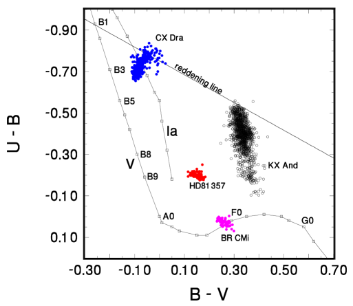
Figure 2: Variations of HD 81357 in the colour - colour diagram are compared to those known for some other Be stars observed at Hvar.

3.3 Reliable radial velocities

3.3.1 phdia RVs

Using the program phdia (see Appendix A), we measured RVs of a number of unblended metallic lines in all blue, red and infrared spectra at our disposal. A period analysis of these RVs confirmed and reinforced the preliminary result of Koubský et al. (2012) that these RVs follow a sinusoidal RV curve with a period of 33$\aas@@fstack{d}$77 and a semi-amplitude of 81 km s^-1. As recently discussed in paper 30 (Harmanec et al. 2015), some caution must be exercised when one analyses binaries with clear signatures of the presence of circumstellar matter in the system. The experience shows that the RV curve of the Roche-lobe filling component is usually clean (with a possible presence of a Rossiter effect) and defines its true orbit quite well, while many of the absorption lines of the mass-gaining component are affected by the presence of circumstellar matter, and their RV curves do not describe the true orbital motion properly. It is therefore advisable to select suitable spectral lines in the blue spectral region, free of such effects.

3.3.2 KOREL maps

In the next step, we therefore derived a map of plausible solutions using a Python program kindly provided by J.A. Nemravová. The program employs the program KOREL, calculates true $\chi^{2}$ values and maps the parameter space to find the optimal values of the semiamplitude $K_{2}$ and the mass ratio $M_{1}/M_{2}$. In our application to HD 81357, we omitted the H$\gamma$ line and used the spectral region 4373 – 4507 Å, which contains several He i and metallic lines of the B-type component 1. As in the case of a similar binary BR CMi (Harmanec et al. 2015) we found that disentangling is not the optimal technique how to derive the most accurate orbital solution since the interplay between a small RV amplitude of the broad-lined B primary and its disentangled line widths results in comparably good fits for a rather wide range of mass ratios. The lowest $\chi^{2}$ was obtained for a mass ratio of 9.75, but there are two other shallow minima near to the mass ratios 7 and 16. The optimal value of $K_{2}$ remained stable near to 81 – 82 km s^-1.

3.3.3 Velocities derived via 2-D cross-correlation

As mentioned earlier, the spectrum of the mass-gaining component is usually affected by the presence of some contribution from circumstellar matter, having a slightly lower temperature than the star itself (e.g. Desmet et al. 2010). This must have impact on KOREL, which disentangles the composite spectra on the premise that all observed spectroscopic variations arise solely from the orbital motion of two binary components. Although we selected a blue spectral region with the exclusion of the H$\gamma$ line (in the hope to minimize the effect of circumstellar matter), it is probable that KOREL solutions returned spectra, which – for the mass-gaining star – average the true stellar spectrum and a contribution from the circumstellar matter.

As an alternative, we decided to derive RVs, which we anyway needed to be able to combine photometry and spectroscopy in the PHOEBE program, with 2-D cross-correlation. We used the asTODCOR program written by one of us (YF) to this goal. The software is based on the method outlined by Zucker & Mazeh (1994) and has already been applied in similar cases (see Desmet et al. 2010; Harmanec et al. 2015, for the details). It performs a 2-D cross-correlation between the composite observed spectra and template spectra. The accuracy and precision of such measurements depend on both, the quality of the observations, and on how suitable templates are chosen to represent the contribution of the two stars.

In what follows, we used the observed blue spectra over the wavelength range from 4370 to 4503 Å, mean resolution 0.12 A mm^-1, and a luminosity ratio $L_{2}/L_{1}=0.1$. We adopted the spectra disentangled by KOREL for the optimal mass ratio 9.75 as the templates for the 2-D cross-correlation. We attempted to investigate the effect of circumstellar matter on the RVs derived with asTODCOR for the primary using also the template spectra for the other two mass ratios derived with KOREL. The RVs are compared in Fig. 3. From it we estimate that, depending on the orbital phase, the systematic error due to the presence of circumstellar matter may vary from 0 to 3 km/s.

The resulting asTODCOR RVs for the optimal mass ratio 9.75 are listed, with their corresponding random error bars, in Table 9 in Appendix, while the SPEFO RVs of the cooler star are in Tab. 10.

Figure 3: Comparison of asTODCOR RVs of star 1 for the optimal mass ratio q=9.75 (solid line) and for the two extreme mass-ratios KOREL templates (q=16 as filled circles, and q=7 as open circles). Typical errors of asTODCOR individual RVs are close to 1.0 km s^-1– see Table 9

Assigning the three sets of asTODCOR RVs from the blue spectral region with the weights inversely proportional to the square of their rms errors, we derived orbital solutions for them. The solutions were derived separately for the hot component 1 and the cool component 2 to verify whether those for the hot star describe its true orbital motion properly. We used the program FOTEL (Hadrava 1990, 2004a). The results are summarised in Table 3. We note that the values of the superior conjunction of component 1 from the separate solutions for component 1 and component 2 agree within their estimated errors, but in all three cases the epochs from component 1 precede a bit those from component 2. This might be another indirect indication that the RVs of component 1 are not completely free of the effects of circumstellar matter.

A disappointing conclusion of this whole exercise is that there is no reliable way how to derive a unique mass ratio from the RVs. One has to find out some additional constraints.

3.4 Trial orbital solutions

Table 3: Trial FOTEL orbital solutions based on asTODCOR RVs from the 18 blue spectra, separately for star 1, and star 2. Circular orbit was assumed and the period was kept fixed at 33$\aas@@fstack{d}$773 d. The solutions were derived using three different RV sets based on the KOREL template spectra for the optimal mass ratio $q$ of 9.75, and for two other plausible mass ratios 7, and 16. The epoch of the superior conjunction $T_{\rm super.\,c.}$ is in RJD-55487 and rms is the rms error of 1 measurement of unit weight.

Element	$q=9.75$	$q=7$	$q=16$
star 1
$T_{\rm super.\,c.}$	0.24(39)	0.50(27)	0.36(64)
$K_{1}$ (km s-1)	8.04(57)	11.09(42)	4.78(92)
rms1 (km s-1)	1.451	1.505	1.441
star 2
$T_{\rm super.\,c.}$	0.617(24)	0.615(24)	0.621(25)
$K_{2}$ (km s-1)	81.82(32)	81.89(32)	81.82(34)
rms2 (km s-1)	0.884	0.887	0.965

In the next step, we derived another orbital solution based on 151 RVs (115 SPEFO RVs, 18 asTODCOR RVs of component 2 and 18 asTODCOR RVs of component 1). As the spectra are quite crowded with numerous lines of component 2, we were unable to use our usual practice of correcting the zero point of the velocity scale via measurements of suitable telluric lines (Horn et al. 1996). That is, why we allowed for the determination of individual systemic velocities for the four subsets of spectra defined in Table 1. All RVs were used with the weights inversely proportional to the square of their rms errors. This solution is in Table 4. There is a very good agreement in the systemic velocities from all individual data subsets, even for the phdia RVs from blue spectra, where only four spectral lines could be measured and averaged.

Table 4: Trial FOTEL orbital solutions based on all 151 phdia and asTODCOR RVs and a solution for the 65 RVs of the H$\alpha$ emission wings measured in SPEFO. The epoch of superior conjunction of star 1 is in RJD, rms is the rms error of 1 observation of unit weight.

Element	Binary	emis. wings H$\alpha$
$P$ (d)	33.77458$\pm$0.00079	33.77458 fixed
$T_{\rm super.\,c.}$	55487.657$\pm$0.020	55492.53$\pm$0.49
$e$	0.0 assumed	0.0 assumed
$K_{1}$ (km s-1)	7.76$\pm$0.56	9.47$\pm$0.88
$K_{2}$ (km s-1)	81.75$\pm$0.17	–
$K_{2}/K_{1}$	0.0949$\pm$0.0063	–
$\gamma_{1}$ (km s-1)	$-$13.46$\pm$0.18	$-$11.33$\pm$0.85
$\gamma_{2}$ (km s-1)	$-$13.04$\pm$0.24	–
$\gamma_{3}$ (km s-1)	$-$13.10$\pm$1.38	–
$\gamma_{4}$ (km s-1)	$-$13.69$\pm$0.25	$-$13.13$\pm$0.74
$\gamma_{\rm 3T1}$ (km s-1)	$-$0.39$\pm$0.37∗	–
$\gamma_{\rm 3T2}$ (km s-1)	$-$0.20$\pm$0.33∗	–
rms (km s-1)	1.138	2.71

3.5 Radiative properties of binary components

To determine the radiative properties of the two binary components, we used the Python program PYTERPOL, which interpolates in a pre-calculated grid of synthetic spectra. Using a set of observed spectra, it tries to find the optimal fit between the observed and interpolated model spectra with the help of a simplex minimization technique. It returns the radiative properties of the system components such as $T_{\rm eff}$, $v$ sin $i$ or $\log\leavevmode\nobreak\ g$, but also the relative luminosities of the stars and RVs of individual spectra.

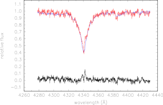
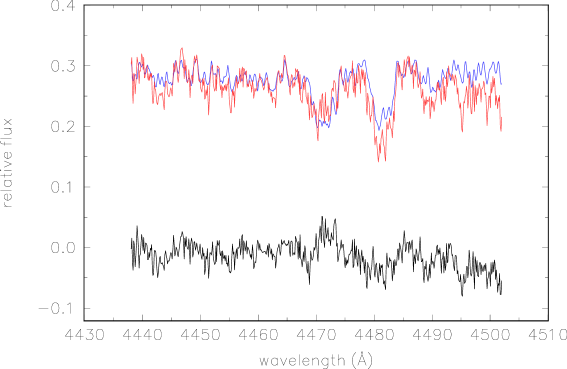
Figure 4: Example of the comparison of an observed blue spectrum in two selected spectral regions with a combination of two synthetic spectra. The residuals in the sense observed minus synthetic are also shown on the same flux scale. To save space, the spectra in the bottom panel were linearly shifted from 1.0 to 0.3 . The H$\gamma$ emission clearly stands out in the residuals in the first panel. See the text for details.

Table 5: Radiative properties of both binary components derived from a comparison of selected wavelength segments of the observed and interpolated synthetic spectra in the blue spectral region.

Element	Component 1	Component 2
$T_{\rm eff}$ (K)	12930$\pm$540	4260$\pm$24
log $g$ [cgs]	4.04$\pm$0.13	2.19$\pm$0.14
$L_{4278-4430}$	0.9570$\pm$0.0092	0.0706$\pm$0.0059
$L_{4438-4502}$	0.9440$\pm$0.0096	0.0704$\pm$0.0075
$v$ sin $i$ (km s-1)	166.4$\pm$1.5	19.7$\pm$0.8

In our particular application, two different grids of spectra were used: AMBRE grid computed by de Laverny et al. (2012) was used for component 2, and the Pollux database computed by Palacios et al. (2010) was used for component 1. We used the 18 file D blue spectra from OND, which contain enough spectral lines of component 1. The following two spectral segments, avoiding the region of the diffuse interstellar band near to 4430 Å, were modelled simultaneously:

4278–4430 Å, and 4438–4502 Å.

Uncertainties of radiative properties were obtained through Markov chain Monte Carlo (MCMC) simulation implemented within emcee Python library by Foreman-Mackey et al. (2013). They are summarised in Table 5 and an example of the fit is in Fig 4. We note that PYTERPOL derives the RV from individual spectra without any assumption about orbital motion. It thus represents some test of the results obtained in the previous analysis based on asTODCOR RVs.

Table 6: Combined radial-velocity curve and light curve solution with PHOEBE. The optimised parameters are given with only their formal errors derived from the covariance matrix.

Element	Orbital properties
$P$ (d)	33.77445$\pm 0.00041$
$T_{\rm sup.c.}$ (RJD)	55487.647$\pm 0.010$
$M_{1}/M_{2}$	10.0$\pm$0.5
$i$ (deg)	63$\pm 5$
$a$ (R⊙)	63.01$\pm$0.09
	Component properties
	Component 1		Component 2
$T_{\rm eff}$  (K)	12930$\pm$540		4260$\pm$24
$\log g_{\rm\left[cgs\right]}$	3.75$\pm$0.15		1.71$\pm$0.25
$M$ ($\mathcal{M}^{\mathrm{N}}_{\odot}$)∗	3.36$\pm$0.15		0.34$\pm$0.04
$R$ ($\mathcal{R}^{\mathrm{N}}_{\odot}$)∗	3.9$\pm$0.2		14.0$\pm$0.7
$F$	30.7$\pm$1.9		1.0 fixed
$L_{\rm U}$	$0.992\pm 0.003$		$0.008\pm 0.003$
$L_{\rm B}$	$0.956\pm 0.003$		$0.044\pm 0.003$
$L_{\rm Hp}$	$0.902\pm 0.004$		$0.098\pm 0.004$
$L_{\rm V}$	$0.853\pm 0.005$		$0.147\pm 0.005$
$L_{\rm V(ASAS)}$	$0.853\pm 0.005$		$0.147\pm 0.005$
$L_{\rm R}$	$0.749\pm 0.007$		$0.251\pm 0.007$

Table 7: $\chi^{2}$ values for individual data sets for the adopted combined PHOEBE solution presented in Table 6.

Data set	No. of	Original	Normalised
	obs.	$\chi^{2}$	$\chi^{2}$
Hvar $U$	27	36.1	1.34
Hvar $B$	27	33.0	1.22
Hvar $V$	27	62.1	2.30
ASAS-SN $V$	209	209.9	1.00
Hipparcos $Hp$	128	176.3	1.38
Hvar $R$	15	22.7	1.51
$RV_{2}$	116	304.1	2.62
Total	549	1063.9	1.94

3.6 Combined light-curve and orbital solution in PHOEBE

To obtain the system properties and to derive the final ephemeris, we used the program PHOEBE  1 (Prša & Zwitter 2005, 2006) and applied it to all photometric observations listed in Table 2 and phdia and asTODCOR RVs for star 2. Since PHOEBE cannot treat different systemic velocities, we used actually RVs minus respective $\gamma$ velocities from the solution listed in Table 4. For the OND blue spectra (file D of Table 1), we omitted the less accurate SPEFO RVs and used only asTODCOR RVs. Bolometric albedos for star 1 and 2 were estimated from Fig. 7 of Claret (2001) as 1.0 and 0.5, respectively. The coefficients of the gravity darkening $\beta$ were similarly estimated as 1.0 and 0.6 from Fig. 7 of Claret (1998).

When we tried to model the light curves on the assumption that the secondary is detached from the Roche lobe, we were unable to model the light-curve amplitudes. We therefore conclude that HD 81357 is a semi-detached binary in the mass transfer phase between the components.

It is not possible to calculate the solution in the usual way. One parameter, which comes into the game, is the synchronicity parameter $F$, which is the ratio between the orbital and rotational period for each component. While it is safe to adopt $F_{2}=1.0$ for the Roche-lobe filling star 2, the synchonicity parameter $F_{1}$ must be re-caculated after each iteration as

$$F_{1}=P_{\rm orbital}{v_{1}\sin i\over{50.59273R_{1}^{\rm e}\sin i}}\,\,,$$ (1)

where the equatorial radius $R_{1}^{\rm e}$ is again in the nominal solar radius $\mathcal{R}^{\mathrm{N}}_{\odot}$, the orbital period in days, and the projected rotational velocity in km s^-1. We adopt the value of 166.4 km s^-1 for $v_{1}\sin i$ from the PYTERPOL solution.

It is usual that there is a very strong parameter degeneracy for an ellipsoidal variable. To treat the problem we fixed $T_{\rm eff}$ of both components obtained from the PYTERPOL solution and used the very accurate parallax of HD 81357 $p=0\aas@@fstack{\prime\prime}0016000\pm 0\aas@@fstack{\prime\prime}0000345$ from the second data release of the Gaia satellite (Gaia Collaboration et al. 2016, 2018) to restrict a plausible range of the solutions.

From a PHOEBE light-curve solution for the Hvar $U\!B{}V$ photometry in the standard Johnson system it was possible to estimate the following $U\!B{}V$ magnitudes of the binary at light maxima

$V_{1+2}=8$${}^{\rm m}\!\!.$321, $B_{1+2}=8$${}^{\rm m}\!\!.$491, and $U_{1+2}=8$${}^{\rm m}\!\!.$300  .

We calculated a number of trial PHOEBE solutions, keeping the parameters of the solution fixed and mapping a large parameter space. For each such solution we used the resulting relative luminosities to derive the $U\!B{}V$ magnitudes of the hot star 1, dereddened them in a standard way and interpolating the bolometric correction from the tabulation of Flower (1996) we derived the range of possible values for the mean radius $R_{1}$ for the Gaia parallax and its range of uncertainty from the formula

$$M_{\rm bol\,1}=42.35326-5\log R_{1}-10\log T_{\rm eff\,1}$$ (2)

(Prša et al. 2016). This range of the radius was compared to the mean radius $R_{1}$ obtained from the corresponding PHOEBE solution. We found that the agreement between these two radius determinations could only be achieved for a very limited range of mass ratios, actually quite close to the mass ratio from the optimal KOREL solution.

The resulting PHOEBE solution is listed in Table 6 and defines the following linear ephemeris, which we shall adopt in the rest of this study

$$T_{\rm super.conj.}={\rm RJD}\,55487.647(10)+33\aas@@fstack{d}77445(41)\times\ E\,.$$ (3)

The fit of the individual light curves is shown in Fig. 5 while in Fig. 6 we compare the fit of the RV curve of component 2 and also the model RV curve of component 1 with the optimal asTODCOR RVs, which however were not used in the PHOEBE solution.

The combined solutions of the light- and RV-curves demonstrated a strong degeneracy among individual parameters. In Table 7 we show the original and normalized $\chi^{2}$ values for the individual data sets used. It is seen that the contribution of the photometry and RVs to the total sum of squares are comparable. A higher $\chi^{2}$ for RVs might be related to the fact that we were unable to compensate small systematic differences in the zero points of RVs between individual spectrographs and/or spectral regions perfectly, having no control via telluric lines. The degeneracy of the parameter space is illustrated by the fact that over a large range of inclinations and tolerable range of mass ratios the program was always able to converge, with the total sum of squares differing by less than three per cent.

Figure 5: $U\!B{}V\!R$ light curves modelled with PHOEBE. Abscissa is labelled with orbital phases according to ephemeris (3).The same scale on ordinate was used to show the changes of the amplitude with passband. For all curves, also the rms errors of individual data points are shown.

Figure 6: Top panels: RV curve of star 2 and the residuals from PHOEBE solution. The rms errors are comparable to the symbols’ size. Bottom panels: asTODCOR RV curve of star 1, not used in the PHOEBE solution, and its residuals from that solution.

In passing we note that we also independently tested the results from PHOEBE using the BINSYN suite of programs (Linnell 1984; Linnell & Hubeny 1996; Linnell 2000) with steepest descent method to optimise the parameters of the binary system (Sudar et al. 2011). This basically confirmed the results obtained with PHOEBE.

4 H$\alpha$ profiles

Figure 7: SPEFO RVs of the H$\alpha$ emission wings with their estimated rms errors plotted vs. orbital phase.

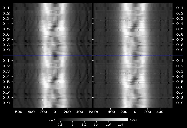
Figure 8: Dynamical spectra in the neighbourhood of the H$\alpha$ profile in a grey-scale representation created in the program phdia. Left-hand panel: observed spectra; right-hand panel: difference spectra after the subtraction of a synthetic spectrum (including the H$\alpha$ profile) of star 2. The phases shown on both sides of the figure, correspond to ephemeris (3). The spectra are repeated over two orbital cycles to show the continuity of the orbital phase changes.

The strength of the H$\alpha$ emission peaks ranges from 1.6 to 2.0 of the continuum level and varies with the orbital phase (cf. Fig. 8). For all spectra a central reversal in the emission is present. But in many cases the absorption structure is quite complicated.

The RV curve of the H$\alpha$ emission wings is well defined, sinusoidal and has a phase shift of some 5 days relative to the RV curve based on the lines of component 1 (see Table 4 and Fig. 7). This must be caused by some asymmetry in the distribution of the circumstellar material producing the emission. In principle, however, one can conclude that the bulk of the material responsible for H$\alpha$ emission moves in orbit with component 1 as it is seen from the semi-amplitude and systemic velocity of the H$\alpha$ emission RV curve, which are similar to those of the component 1. We note that in both, the magnitude and sense of the phase shift, this behaviour is remarkably similar to that of another emission-line semi-detached binary AU Mon (Desmet et al. 2010).

The orbital variation of the H$\alpha$ emission-line profiles in the spectrum of HD 81357 is illustrated in the dynamical spectra created with the program phdia – see the left panel of Fig. 8. The lines of the cool component are seen both shorward and longward of the H$\alpha$ emission. These lines can be used to trace the motion of H$\alpha$ absorption originating from star 2. It is readily seen that the behaviour of the central absorption in the H$\alpha$ emission is more complicated than what would correspond to the orbital motion of star 2. Three stronger absorption features can be distinguished: region 1 near to phase 0.0, region 2 visible from phase 0.4 to 0.5, and somewhat fainter feature 3 present between phases 0.65 and 0.85. The absorption in region 2 follows the motion of star 2, while the absortion line in region 3 moves in antiphase.

In the right panel of Fig. 8 we show the dynamical spectra of the difference profiles resulting after subtraction of an interpolated synthetic spectrum of star 2 (properly shifted in RV according to the orbital motion of star 2) from the observed H$\alpha$ profiles. We note that the lines of star 2 disappeared, but otherwise no pronounced changes in the H$\alpha$ profiles occurred in comparison to the original ones. Thus, the regions of enhanced absorption 1, 2, and 3, already seen on the original profiles are phase-locked and must be connected with the distribution of circumstellar matter in the system.

There are two principal possible geometries of the regions responsible for the H$\alpha$ emission: Either an accretion disk, the radius of which would be limited by the dimension of the Roche lobe around the hot star, $\sim 37$ $\mathcal{R}^{\mathrm{N}}_{\odot}$ for our model; or a bipolar jet perpendicular to the orbital plane, known, for instance, for $\beta$ Lyr (Harmanec et al. 1996), V356 Sgr, TT Hya, and RY Per (Peters & Polidan 2007) or V393 Sco (Mennickent et al. 2012), originating from the interaction of the gas stream encircling the hot star with the denser stream flowing from the Roche-lobe filling star 2 towards star 1 (Bisikalo et al. 2000). In passing we note that no secular change in the strength of the H$\alpha$ emission over the interval covered by the data could be detected.

5 Stellar evolution of HD 81357 with mass exchange

Given a rather low mass and a large radius of the secondary, we were interested to test whether stellar evolution with mass exchange in a binary can produce a system similar to HD 81357. We use the binary stellar evolution program MESA (Paxton et al. 2011, 2015) in order to test a certain range of input parameters. We tried the initial masses in the intervals $M_{1}\in(1.0;1.5)\,\hbox{$\mathcal{M}^{\mathrm{N}}_{\odot}$}$, $M_{2}\in(2.2;2.7)\,\hbox{$\mathcal{M}^{\mathrm{N}}_{\odot}$}$, and the initial binary period $P\in(2;10)\,{\rm days}$. Hereinafter, we use the same notation as in the preceding text, so that $M_{1}$ is the original secondary, which becomes the primary during the process of mass exchange. The mass transfer was computed with Ritter (1988) explicit scheme, with the rate limited to $\dot{M}_{\rm max}=10^{-7}\,\hbox{$\mathcal{M}^{\mathrm{N}}_{\odot}$},{\rm yr}^{-1}$, and magnetic breaking of Rappaport et al. (1983), with the exponent $\gamma=3$. For simplicity, we assumed zero eccentricity, conservative mass transfer, no tidal interactions, and no irradiation. We used the standard time step controls.

An example for the initial masses $M_{1}=1.5\,\hbox{$\mathcal{M}^{\mathrm{N}}_{\odot}$}$, $M_{2}=2.2\,\hbox{$\mathcal{M}^{\mathrm{N}}_{\odot}$}$, the initial period $P=2.4\,{\rm d}$ and the mass transfer beginning on the SGB is presented in Figure 9. We obtained a result, which matches the observations surprisingly well, namely the final semimajor axis $a_{\rm syn}=66.04\,\hbox{$\mathcal{R}^{\mathrm{N}}_{\odot}$}$, which corresponds to the period $P_{\rm syn}\doteq 32.60\,{\rm d}$ (while $P_{\rm obs}=33.77\,{\rm d}$), the final masses $M_{1}=3.37\,\hbox{$\mathcal{M}^{\mathrm{N}}_{\odot}$}$ ($3.36\,\hbox{$\mathcal{M}^{\mathrm{N}}_{\odot}$}$), $M_{2}=0.33\,\hbox{$\mathcal{M}^{\mathrm{N}}_{\odot}$}$ ($0.34\,\hbox{$\mathcal{M}^{\mathrm{N}}_{\odot}$}$), the maximum secondary radius $R_{2}=13.1\,\hbox{$\mathcal{R}^{\mathrm{N}}_{\odot}$}$ ($14.0\,\hbox{$\mathcal{R}^{\mathrm{N}}_{\odot}$}$), with the exception of the primary radius $R_{1}=2.3\,\hbox{$\mathcal{R}^{\mathrm{N}}_{\odot}$}$ (cf. $3.9\,\hbox{$\mathcal{R}^{\mathrm{N}}_{\odot}$}$). Alternatively, solutions can be also found for different ratios of the initial masses $M_{1}$, $M_{2}$, and later phases of mass transfer (RGB), although they are sometimes preceded by an overflow. An advantage may be an even better fit of the final $R_{1}$, and a relatively longer duration of the inflated $R_{2}$ which makes such systems more likely to be observed.

Consequently, we interpret the secondary as a low-mass star with a still inflated envelope, close to the end of the mass transfer phase. We demonstrated that a binary with an ongoing mass transfer is a reasonable explanation for both components of the HD 81357 system. A more detailed modelling including an accretion disk, as carried out by Van Rensbergen & De Greve (2016) for other Algols, would be desirable.

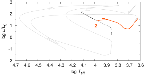
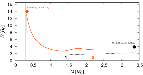
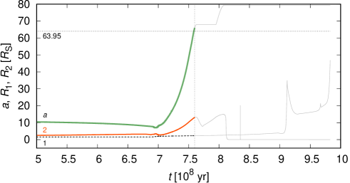
Figure 9: Long-term evolution of HD 81357 binary as computed by MESA (Paxton et al. 2015). The initial masses were $M_{1}=1.5\,M_{\odot}$, $M_{2}=2.2\,M_{\odot}$, and the initial period $P=2.4\,{\rm d}$. Top: the HR diagram with the (resulting) primary denoted as 1 (dashed black line), secondary as 2 (solid orange line) at the beginning of the evolutionary tracks (ZAMS). Middle: the radius $R$ vs mass $M$; the corresponding observed values are also indicated (filled circles). Bottom: the semimajor axis $a$ of the binary orbit (green) and the radii $R_{1}$, $R_{2}$ of the components vs time $t$. The observed value $a=63.95\,R_{\odot}$ and the time $t\doteq 7.6\cdot 10^{8}\,{\rm yr}$ with the maximal $R_{2}$ are indicated (thin dotted). Later evolutionary phases are also plotted (solid grey line).

6 Discussion

Quite many of similar systems with a hot mass-gaining component were found to exhibit cyclic long-term light and colour variations, with cycles an order of magnitude longer than the respective orbital periods (cf. a good recent review by Mennickent 2017), while others seem to have a constant brightness outside the eclipses. The later seems to be the case of HD 81357, for which we have not found any secular changes. It is not clear as yet what is the principal factor causing the presence of the cyclic secular changes (see also the discussion in Harmanec et al. 2015). A few yellow-band photoelectric observations of HD 81357 found in the literature all give 8${}^{\rm m}\!\!.$3 to 8${}^{\rm m}\!\!.$4. It is notable, however, that both magnitudes given in the HD catalogue are 7${}^{\rm m}\!\!.$9. Future monitoring of the system brightness thus seems desirable.

We note that we have not found any indication of a secular period change and also our modelling of the system evolution and its low mass ratio $M_{2}/M_{1}$ seem to indicate that HD 81357 is close to the end of mass exchange process. The same is also true about BR CMi studied by Harmanec et al. (2015). We can thus conjecture that the cyclic light variations mentioned above do not occur close to the end of the mass exchange.

Appendix A Details of the spectral data reduction and measurements

The initial reduction of all OND and DAO spectra (bias subtraction, flat-fielding, creation of 1-D spectra, and wavelength calibration) was carried out in IRAF. Optimal extraction was used. Normalization, removal of residual cosmics and flaws and RV measurements of H$\alpha$ emission profiles were carried out with the program SPEFO (Horn et al. 1996; Škoda 1996), namely the latest version 2.63 developed by Mr. J. Krpata (Krpata 2008). SPEFO displays direct and flipped traces of the line profiles superimposed on the computer screen that the user can slide to achieve a precise overlapping of the parts of the profile of whose RV one wants to measure. RVs of a selection of stronger unblended lines of the cool component 2 (see Table 8) covering the red and infrared spectral regions (available for all spectra), were measured using the program phdia written by LK. The program phdia is a web application which allows the creation of dynamical spectra and, using a similar principle as the program SPEFO, also RV measurements based on the comparison of direct and flipped line profiles. The input is a normalized digital spectrum. A robust mean RV with the rms error was derived for each spectrum to obtain the mean RV. In contrast to our usual approach, we have not measured a selection of good telluric lines to obtain an additional fine correction of the RV zero point of each spectrogram because of a strong blending of the telluric lines with the stellar lines of the cool component 2. Moreover, we measured the RVs of the steep wings of the H$\alpha$ emission line repeatably at different times to obtain an estimate of the rms error for these measurements. We point out that although some broad and shallow lines of component 1 are seen in the spectra, their direct RV measurement is impossible because of numerous blends with the lines of component 2.

Table 8: List of spectral lines of component 2 and their air wavelengths used for the RV measurements in phdia. The numbering of the multiplets of individual ions corresponds to the one introduced by Moore (1945). The wavelengths are taken from the NIST Atomic Spectra Database. In some cases, weighted mean of the wavelengths of close blends in the neighborhood of the line in question was used (such cases are denoted by letter ”c”).

Wavelength	Element	Wavelength	Element
(Å)		(Å)
4425.824	Ti i 78	6624.912	Fe i 13 c
4427.310	Fe i 2	6633.749	Fe i 1197
4430.189	Fe i 472	6643.638	Ni i 43
4454.780	Ca i 4	6663.442	Fe i 111
6322.685	Fe i 207	6677.986	Fe i 268 c
6327.450	Cr i	6717.690	Ca i 1194
6338.999	Fe i 1258 c	8426.504	Ti i 33
6344.149	Fe i 169	8468.407	Fe i 60
6355.029	Fe i 342	8582.257	Fe i 401
6358.697	Fe i 13	8611.803	Fe i 339
6366.424	Ti i 103 c	8621.600	Fe i 401
6393.601	Fe i 168	8648.462	Si i
6400.147	Fe i 816+13 c	8662.140	Ca ii
6408.018	Fe i 816	8674.985	Fe i
6411.649	Fe i 816	8688.625	Fe i 60
6419.872	Fe i 1258	8710.391	Fe i 1267
6421.350	Fe i 111	8757.187	Fe i 339
6430.846	Fe i 62	8763.966	Fe i 1172
6439.070	Ca i 18	8793.343	Fe i 1172
6462.658	Ca i 18	8806.757	Mg i 7
6471.660	Ca i 18	8824.221	Fe i 60
6613.756	Fe i c	8838.428	Fe i 339
		8866.932	Fe i 1172

Table 9: Individual asTODCOR RVs of the hot component 1 and cool component 2 derived from the 18 file D spectra in the blue spectral region 4370 - 4503 Å (columns 2 and 3), using the KOREL template for $q=0.975$, and phdia RVs of component 2 (column 4).

RJD	RV1	RV2	RV${}_{2}^{{\tt SPEFO}}$
	(km s-1)	(km s-1)	(km s-1)
56765.3585	$7.47\pm 0.99$	$-71.72\pm 0.61$	$-94.00\pm 5.15$
56769.4557	$1.45\pm 1.19$	$-22.17\pm 0.69$	$-30.83\pm 3.91$
56771.4295	$0.38\pm 0.99$	$7.07\pm 0.80$	$-3.78\pm 2.68$
56778.3392	$-6.81\pm 1.19$	$78.73\pm 0.63$	$70.07\pm 5.14$
56782.4491	$-8.11\pm 1.59$	$69.74\pm 1.59$	–
56797.4027	$5.08\pm 1.01$	$-79.91\pm 0.48$	$-96.32\pm 1.82$
56799.3612	$4.20\pm 1.36$	$-69.34\pm 0.80$	$-85.33\pm 0.65$
56809.4039	$-8.85\pm 0.99$	$61.11\pm 0.68$	$48.81\pm 0.97$
56814.4188	$-10.09\pm 1.14$	$78.99\pm 0.73$	$63.61\pm 1.66$
56815.4057	$-6.01\pm 1.05$	$75.10\pm 0.52$	$61.20\pm 1.94$
56816.4472	$-7.53\pm 0.88$	$67.75\pm 0.72$	$59.85\pm 2.34$
56817.3872	$-4.00\pm 0.88$	$58.16\pm 0.55$	$45.85\pm 3.74$
56818.3936	$-6.26\pm 0.90$	$48.52\pm 0.60$	$40.45\pm 1.35$
56824.3882	$4.59\pm 1.36$	$-41.11\pm 1.04$	$-49.37\pm 1.46$
56827.3853	$7.66\pm 1.08$	$-73.04\pm 0.60$	$-85.43\pm 4.14$
56831.4217	$7.35\pm 1.20$	$-78.75\pm 0.83$	$-88.40\pm 1.99$
56835.3919	$3.75\pm 1.05$	$-44.89\pm 0.68$	$-55.12\pm 4.26$
56853.3661	$-2.04\pm 0.85$	$29.70\pm 0.68$	$25.21\pm 6.86$

Table 10: Individual RVs of the cool component 2 and of the H$\alpha$ emission wings (RV${}_{\rm H\alpha\ em.}$) from the red and IR spectra measured in phdia and SPEFO. Individual files are identified by their file codes from Table 1.

RJD	RV2	RV${}_{\rm H\alpha\ em.}$	Spg.	RJD	RV2	RV${}_{\rm H\alpha\ em.}$	Spg.
	(km s-1)	(km s-1)			(km s-1)	(km s-1)
55621.5844	$-31.00\pm 0.31$	$-4.79\pm 0.77$	A/1	55740.4180	$-2.17\pm 0.60$	–	C/2
55644.4775	$-79.07\pm 0.63$	$-10.76\pm 0.29$	A/1	55750.3954	$-92.50\pm 0.63$	–	C/2
55661.4801	$51.43\pm 0.56$	$-19.97\pm 0.87$	A/1	55751.3787	$-88.36\pm 0.40$	–	C/2
55672.4335	$1.89\pm 0.41$	$-27.67\pm 0.50$	A/1	55754.3639	$-60.93\pm 0.71$	–	C/2
55691.5362	$6.19\pm 0.35$	$-5.54\pm 0.17$	A/1	55759.3896	$10.68\pm 0.50$	–	C/2
55693.4009	$30.16\pm 0.46$	$-12.68\pm 0.77$	A/1	55808.6067	$-12.40\pm 0.62$	–	C/2
55703.3408	$40.36\pm 0.45$	$-26.35\pm 0.28$	A/1	55817.5587	$-93.63\pm 0.86$	–	C/2
55707.3493	$-16.37\pm 0.66$	$-22.57\pm 0.81$	A/1	55831.6385	$61.31\pm 0.46$	–	C/2
55742.4201	$-36.56\pm 0.56$	$-15.79\pm 0.56$	A/1	56007.4786	$40.66\pm 0.50$	–	C/2
55749.3717	$-94.36\pm 0.52$	$-3.83\pm 1.21$	A/1	56012.4986	$-35.32\pm 0.63$	–	C/2
55752.3664	$-80.57\pm 0.56$	$0.82\pm 0.41$	A/1	56044.4130	$-4.28\pm 0.57$	–	C/2
55807.5902	$2.00\pm 0.63$	$-18.92\pm 1.33$	A/1	56045.3781	$-21.21\pm 0.43$	–	C/2
55817.5303	$-95.16\pm 0.51$	$0.28\pm 2.01$	A/1	56046.4416	$-37.25\pm 0.65$	–	C/2
55836.5069	$60.10\pm 0.48$	$-16.36\pm 0.15$	A/1	56642.6600	$63.16\pm 0.32$	–	C/2
55877.5068	$-36.76\pm 0.56$	$-19.85\pm 0.78$	A/1	56771.3714	$-8.29\pm 0.49$	–	C/2
55969.5233	$67.82\pm 0.60$	$-16.18\pm 0.76$	A/1	56797.3361	$-94.94\pm 0.56$	–	C/2
56007.5227	$38.30\pm 0.45$	$-22.38\pm 0.34$	A/1	56810.4372	$57.67\pm 0.55$	–	C/2
56008.4721	$27.50\pm 0.46$	$-21.95\pm 0.77$	A/1	56818.3462	$36.93\pm 0.58$	–	C/2
56011.5609	$-20.15\pm 0.66$	$-20.67\pm 1.24$	A/1	57070.6612	$-71.38\pm 0.60$	–	C/2
56013.4972	$-49.70\pm 0.48$	$-14.73\pm 0.28$	A/1	57073.4943	$-37.73\pm 1.04$	–	C/2
56015.4132	$-73.31\pm 0.70$	$-9.26\pm 0.54$	A/1	57117.3562	$68.45\pm 0.46$	–	C/2
56044.4414	$-4.95\pm 0.58$	$-22.62\pm 0.79$	A/1	57118.4756	$65.64\pm 0.38$	–	C/2
56045.3434	$-20.13\pm 0.56$	$-20.51\pm 0.65$	A/1	55680.7562	$-94.71\pm 0.48$	$-10.63\pm 0.21$	E/4
56046.4681	$-37.62\pm 0.52$	$-18.22\pm 1.08$	A/1	55681.7524	$-95.77\pm 0.60$	$-4.56\pm 0.40$	E/4
56235.4193	$49.07\pm 0.65$	$-12.34\pm 0.74$	A/1	55682.7582	$-94.65\pm 0.50$	$-6.07\pm 0.58$	E/4
56433.3847	$-12.56\pm 0.54$	$-5.46\pm 0.65$	A/1	55685.7612	$-73.64\pm 0.44$	$-1.54\pm 0.40$	E/4
56642.6053	$63.54\pm 0.43$	$-18.53\pm 1.04$	B/1	55735.7331	$58.02\pm 1.40$	–	E/4
56712.5061	$67.66\pm 0.51$	$-18.45\pm 0.84$	B/1	55859.9161	$-3.46\pm 0.47$	$-4.07\pm 0.79$	E/4
56718.4552	$17.03\pm 0.36$	$-22.20\pm 0.66$	B/1	55953.9582	$-90.56\pm 0.45$	$-5.74\pm 0.85$	E/4
56746.4230	$67.52\pm 0.50$	$-20.29\pm 0.66$	B/1	55993.9278	$-19.21\pm 0.35$	$-1.69\pm 1.11$	E/4
56759.3533	$-81.82\pm 0.71$	$-9.43\pm 0.21$	B/1	56034.7448	$62.65\pm 0.34$	$-16.83\pm 0.44$	E/4
56764.3167	$-91.72\pm 0.55$	$-4.03\pm 0.46$	B/1	56034.7806	$62.22\pm 0.48$	$-15.19\pm 0.24$	E/4
57074.4891	$-21.74\pm 0.61$	$-5.00\pm 0.34$	B/1	56072.7588	$60.14\pm 0.51$	$-18.65\pm 1.24$	E/4
57080.5153	$54.84\pm 0.50$	$-19.44\pm 0.67$	B/1	56073.7163	$51.22\pm 0.40$	$-20.46\pm 0.82$	E/4
57101.6119	$-92.96\pm 0.57$	$1.36\pm 0.82$	B/1	56073.7926	$51.93\pm 0.40$	$-19.91\pm 0.56$	E/4
57105.3867	$-62.06\pm 0.51$	$-4.92\pm 0.70$	B/1	56074.7968	$42.03\pm 1.12$	–	E/4
57106.4352	$-49.53\pm 0.39$	$-4.57\pm 0.45$	B/1	56113.7894	$-34.91\pm 0.44$	$-21.87\pm 1.18$	E/4
57116.4673	$66.46\pm 0.64$	$-17.40\pm 0.58$	B/1	56296.0908	$-44.65\pm 0.44$	$-7.17\pm 0.96$	E/4
57117.3111	$67.46\pm 0.52$	$-19.30\pm 0.46$	B/1	56379.9514	$27.72\pm 0.51$	$-22.91\pm 0.86$	E/4
57118.5416	$65.79\pm 0.52$	$-20.62\pm 0.40$	B/1	56380.9409	$13.71\pm 0.37$	$-23.57\pm 0.49$	E/4
55621.6176	$-29.52\pm 0.40$	–	C/2	56384.9173	$-48.98\pm 0.39$	$-16.53\pm 0.25$	E/4
55645.5398	$-86.02\pm 0.64$	–	C/2	56408.8349	$67.06\pm 0.50$	$-15.47\pm 1.02$	E/4
55662.4553	$59.10\pm 0.56$	–	C/2	56410.8205	$57.49\pm 0.49$	$-19.28\pm 0.64$	E/4
55663.4181	$64.29\pm 0.43$	–	C/2	56444.7391	$56.99\pm 0.58$	$-17.79\pm 0.98$	E/4
55691.5822	$4.30\pm 0.64$	–	C/2	56446.7468	$36.02\pm 0.61$	$-24.52\pm 1.04$	E/4
55693.3831	$30.23\pm 0.50$	–	C/2	56787.7054	$-9.58\pm 0.50$	$-25.48\pm 0.37$	E/4
55703.3784	$40.97\pm 0.62$	–	C/2	56817.7530	$42.84\pm 0.52$	$-25.79\pm 0.92$	E/4
55704.4937	$28.33\pm 0.63$	–	C/2	56818.7358	$31.25\pm 0.48$	$-27.35\pm 1.02$	E/4
55707.3759	$-15.42\pm 0.57$	–	C/2	56819.7342	$17.45\pm 0.52$	$-24.22\pm 0.53$	E/4

Appendix B Details on the photometric data used

Below, we provide some details of the individual data sets and their reductions.

• Station 01 – Hvar:   These differential $U\!B{}V$ and later $U\!B{}V\!R$ observations have been secured by HB, PH, and DR relative to HD 82861 (the check star HD 81772 being observed as frequently as the variable) and carefully transformed to the standard $UBV(R)$ system via non-linear transformation formulæ using the HEC22 reduction program – see Harmanec et al. (1994) and Harmanec & Horn (1998) for the observational strategy and data reduction. All observations were reduced with the latest HEC22 rel.18 program, which allows the time variation of linear extinction coefficients to be modelled in the course of observing nights. For the light-curve solutions we used normal points averaged over the typical observing sequence of 0$\aas@@fstack{d}$055 and the corresponding rms errors.

• Station 61 – Hipparcos:   These all-sky observations were reduced to the standard $V$ magnitude via the transformation formulæ derived by Harmanec (1998) to verify that no secular light changes in the system were observed. However, for the light-curve solution in PHOEBE, we consider the Hipparcos transmission curve for the $H_{p}$ magnitude and also use the original rms errors.

• Station 93 – ASAS-SN:   These all-sky automated survey for supernovae $V$ observations were adopted from the data server https://asan-sn.osu.edu (Shappee et al. 2014; Kochanek et al. 2017) and cleaned for some strongly deviating data points. We used only the observations from the bb camera, which were numerous enough. The rms errors provided by the on the fly calculator are unrealistically small (cf. Jayasinghe et al. 2019) and we used them only to assign relative weights to individual observations, inversely proportional to their square and estimated the mean rms scatter as 0.0065 mag.

Journal of all data sets is in Table 2.

Table 11: Individual $U\!B{}V\!R$ observations from the Hvar Observatory. The comparison star was HD 82861, for which we used the mean Hvar all-sky values $V=7$${}^{\rm m}\!\!.$073, $B\!-\!V$ $=$ 0${}^{\rm m}\!\!.$141, $U\!-\!B$ $=$ 0${}^{\rm m}\!\!.$093, and $V\!-\!R$ $=$ 0${}^{\rm m}\!\!.$129. $X$ is the air mass of the observation and $\bigtriangleup$X = X${}_{\rm var.}-$X_comp. is the air-mass difference between the variable and comparison star.

RJD	weight	$V$	$B$	$U$	$R$	$B\!-\!V$	$U\!-\!B$	X	$\bigtriangleup$X
		(mag.)	(mag.)	(mag.)	(mag.)	(mag.)	(mag.)
55879.6237	1.50	8.349	8.509	8.301	–	0.160	-0.208	1.088	-0.005
55879.6307	1.50	8.351	8.507	8.296	–	0.156	-0.211	1.079	-0.004
55879.6340	1.50	8.353	8.501	8.300	–	0.148	-0.201	1.075	-0.004
55881.6675	1.50	8.339	8.499	8.311	–	0.160	-0.188	1.042	0.002
55881.6724	1.50	8.334	8.489	8.299	–	0.155	-0.190	1.040	0.002
55881.6756	1.50	8.330	8.499	8.308	–	0.169	-0.191	1.039	0.003
55938.4882	1.50	8.348	8.500	8.304	–	0.152	-0.196	1.061	-0.002
55938.4946	1.50	8.347	8.497	8.299	–	0.150	-0.198	1.056	-0.001
55938.4994	1.50	8.343	8.497	8.301	–	0.154	-0.196	1.052	-0.000
55939.4333	1.50	8.351	8.497	8.302	–	0.146	-0.195	1.137	-0.011
55939.4403	1.50	8.345	8.503	8.301	–	0.158	-0.202	1.124	-0.009
55939.4438	1.50	8.356	8.505	8.306	–	0.149	-0.199	1.118	-0.009
55942.4879	1.50	8.383	8.515	8.297	–	0.132	-0.218	1.052	-0.000
55942.4944	1.50	8.377	8.511	8.300	–	0.134	-0.211	1.048	0.000
55942.4976	1.50	8.380	8.510	8.304	–	0.130	-0.206	1.046	0.001
55943.4734	1.50	8.378	8.510	8.301	–	0.132	-0.209	1.063	-0.002
55943.4797	1.50	8.387	8.513	8.306	–	0.126	-0.207	1.057	-0.001
55943.4829	1.50	8.379	8.504	8.303	–	0.125	-0.201	1.054	-0.001
56001.3532	1.50	8.332	8.492	8.307	–	0.160	-0.185	1.037	0.003
56001.3600	1.50	8.333	8.498	8.303	–	0.165	-0.195	1.036	0.004
56001.3633	1.50	8.327	8.497	8.310	–	0.170	-0.187	1.035	0.004
56002.3781	1.50	8.323	8.481	8.294	–	0.158	-0.187	1.035	0.006
56002.3842	1.50	8.327	8.489	8.303	–	0.162	-0.186	1.037	0.007
56002.3873	1.50	8.315	8.484	8.289	–	0.169	-0.195	1.038	0.007
56013.3318	0.50	8.379	8.503	8.293	–	0.124	-0.210	1.035	0.004
56013.3364	0.50	8.361	8.505	8.297	–	0.144	-0.208	1.035	0.005
56013.3394	0.50	8.372	8.515	8.310	–	0.143	-0.205	1.035	0.005
56015.3404	0.50	8.337	8.499	8.320	–	0.162	-0.179	1.035	0.006
56015.3451	0.50	8.349	8.518	8.327	–	0.169	-0.191	1.036	0.006
56015.3482	0.50	8.347	8.491	8.299	–	0.144	-0.192	1.037	0.007
56065.3231	1.00	8.359	8.508	8.291	–	0.149	-0.217	1.186	0.017
56065.3294	1.00	8.366	8.504	8.293	–	0.138	-0.211	1.202	0.018
56065.3324	1.00	8.373	8.510	8.300	–	0.137	-0.210	1.211	0.018
56086.3506	1.00	8.314	8.498	8.307	–	0.184	-0.191	1.516	0.024
56086.3555	1.00	8.327	8.496	8.314	–	0.169	-0.182	1.543	0.024
56086.3590	1.00	8.312	8.488	8.301	–	0.176	-0.187	1.563	0.025
56747.3537	1.00	8.313	8.481	8.295	8.147	0.168	-0.186	1.040	0.008
56747.3712	1.00	8.319	8.489	8.308	8.133	0.170	-0.181	1.050	0.009
56747.3754	1.00	8.322	8.498	8.310	8.148	0.176	-0.188	1.053	0.010
56755.3233	1.00	8.370	8.508	8.303	8.228	0.138	-0.205	1.037	0.007
56755.3318	1.00	8.371	8.497	8.299	8.232	0.126	-0.198	1.040	0.008
56755.3359	1.00	8.370	8.492	8.292	8.207	0.122	-0.200	1.042	0.008
56757.3444	1.00	8.340	8.497	8.288	8.169	0.157	-0.209	1.051	0.009
56757.3523	1.00	8.357	8.499	8.305	8.194	0.142	-0.194	1.057	0.010
56757.3563	1.00	8.357	8.499	8.300	8.206	0.142	-0.199	1.061	0.011
56759.2984	0.50	8.332	8.500	8.306	8.177	0.168	-0.194	1.035	0.005
56759.3074	0.50	8.336	8.489	8.298	8.170	0.153	-0.191	1.036	0.006
56759.3130	0.50	8.323	8.486	8.296	8.163	0.163	-0.190	1.037	0.007
56761.3048	1.00	8.310	8.480	8.301	8.149	0.170	-0.179	1.037	0.007
56761.3107	1.00	8.308	8.485	8.308	8.124	0.177	-0.177	1.038	0.007

Table 1: continued

RJD	weight	$V$	$B$	$U$	$R$	$B\!-\!V$	$U\!-\!B$	X	$\bigtriangleup$X
		(mag.)	(mag.)	(mag.)	(mag.)	(mag.)	(mag.)
56761.3175	1.00	8.320	8.489	8.306	8.141	0.169	-0.183	1.041	0.008
56804.3396	1.00	8.387	8.502	8.309	8.221	0.115	-0.193	1.309	0.021
56804.3462	1.00	8.384	8.515	8.310	8.229	0.131	-0.205	1.334	0.022
56804.3533	1.00	8.386	8.525	8.306	8.225	0.139	-0.219	1.362	0.022
56812.3428	1.00	8.319	8.497	8.313	8.135	0.178	-0.184	1.414	0.023
56812.3445	1.00	8.327	8.505	8.316	8.148	0.178	-0.189	1.422	0.023
56812.3506	1.00	8.307	8.464	8.279	8.132	0.157	-0.185	1.451	0.023
56858.3315	1.00	8.377	8.538	8.320	8.173	0.161	-0.218	2.307	0.014
56858.3393	1.00	8.364	8.518	8.301	8.182	0.154	-0.217	2.403	0.010
56858.3441	1.00	8.375	8.547	8.297	8.170	0.172	-0.250	2.464	0.007
56867.3311	1.00	8.334	8.503	8.286	8.161	0.169	-0.217	2.622	-0.002
56867.3372	1.00	8.344	8.506	8.310	8.168	0.162	-0.196	2.709	-0.007
56867.3393	1.00	8.339	8.493	8.293	8.195	0.154	-0.200	2.740	-0.009
56873.3170	0.50	8.390	8.505	8.289	8.224	0.115	-0.216	2.652	-0.003
56873.3190	0.50	8.363	8.496	8.299	8.231	0.133	-0.197	2.681	-0.005
56873.3257	0.50	8.379	8.529	8.300	8.206	0.150	-0.229	2.782	-0.012
57100.3264	1.00	8.325	8.492	8.311	8.145	0.167	-0.181	1.045	0.001
57100.3281	1.00	8.316	8.483	8.303	8.135	0.167	-0.180	1.044	0.001
57100.3327	1.00	8.327	8.486	8.300	8.125	0.159	-0.186	1.042	0.002
57100.3344	1.00	8.328	8.485	8.304	8.124	0.157	-0.181	1.041	0.002
57100.3409	1.00	8.334	8.500	8.320	8.153	0.166	-0.180	1.038	0.003
57100.3426	1.00	8.333	8.511	8.324	8.137	0.178	-0.187	1.038	0.003
57101.2961	1.00	8.326	8.488	8.307	8.153	0.162	-0.181	1.068	-0.003
57101.2978	1.00	8.321	8.488	8.303	8.136	0.167	-0.185	1.067	-0.003
57101.3064	1.00	8.332	8.495	8.313	8.154	0.163	-0.182	1.058	-0.001
57101.3082	1.00	8.339	8.501	8.326	8.160	0.162	-0.175	1.057	-0.001
57101.3157	1.00	8.334	8.493	8.307	8.146	0.159	-0.186	1.051	-0.000
57101.3210	1.00	8.335	8.502	8.314	8.134	0.167	-0.188	1.047	0.001
57114.3361	1.00	8.335	8.487	8.301	8.187	0.152	-0.186	1.036	0.006
57114.3454	1.00	8.330	8.493	8.293	8.179	0.163	-0.200	1.039	0.007
57114.3521	1.00	8.351	8.489	8.297	8.189	0.138	-0.192	1.041	0.008
57114.3588	1.00	8.340	8.503	8.299	8.155	0.163	-0.204	1.045	0.009
57114.3662	1.00	8.336	8.504	8.300	8.168	0.168	-0.204	1.050	0.009
57114.3730	1.00	8.335	8.496	8.310	8.183	0.161	-0.186	1.055	0.010
57115.3537	1.00	8.332	8.493	8.286	8.156	0.161	-0.207	1.044	0.008
57115.3605	1.00	8.330	8.498	8.310	8.170	0.168	-0.188	1.048	0.009
57115.3669	1.00	8.348	8.490	8.294	8.156	0.142	-0.196	1.052	0.010
57115.3734	1.00	8.334	8.487	8.287	8.165	0.153	-0.200	1.058	0.010
57115.3799	1.00	8.331	8.491	8.297	8.174	0.160	-0.194	1.064	0.011
57116.3552	0.50	8.294	8.454	8.264	8.205	0.160	-0.190	1.046	0.009
57116.3614	0.50	8.313	8.481	8.289	8.220	0.168	-0.192	1.050	0.009
57116.3676	0.50	8.294	8.455	8.257	8.246	0.161	-0.198	1.055	0.010
57116.3755	0.50	8.308	8.472	8.277	8.237	0.164	-0.195	1.062	0.011