Relighting Humans: Occlusion-Aware Inverse Rendering for Full-Body Human Images

Abstract.

Relighting of human images has various applications in image synthesis. For relighting, we must infer albedo, shape, and illumination from a human portrait. Previous techniques rely on human faces for this inference, based on spherical harmonics (SH) lighting. However, because they often ignore light occlusion, inferred shapes are biased and relit images are unnaturally bright particularly at hollowed regions such as armpits, crotches, or garment wrinkles. This paper introduces the first attempt to infer light occlusion in the SH formulation directly. Based on supervised learning using convolutional neural networks (CNNs), we infer not only an albedo map, illumination but also a light transport map that encodes occlusion as nine SH coefficients per pixel. The main difficulty in this inference is the lack of training datasets compared to unlimited variations of human portraits. Surprisingly, geometric information including occlusion can be inferred plausibly even with a small dataset of synthesized human figures, by carefully preparing the dataset so that the CNNs can exploit the data coherency. Our method accomplishes more realistic relighting than the occlusion-ignored formulation.

Figure 1. Given a single human image and its mask, our method infers a light transport map (i.e., coefficient vectors of second-order spherical harmonics that encode light occlusion), light, and albedo map using convolutional neural networks, and allows fast relighting of the human figure under different illuminations with self-shadows. Input image courtesy of Jose Martinez.

1. Introduction

Relighting of human images has various applications in image synthesis such as stylized shading of portraits [Chai et al., 2015; Shu et al., 2017a] or cut & paste of human image clips [Xue et al., 2012]. For physically-based relighting of a human portrait, we must infer reflectance, shape, and illumination from the single image. Previous techniques obtain the cues of albedo and shape from human faces via fitting of morphable 3D face models [Blanz and Vetter, 1999] or inference based on convolutional neural networks (CNNs) [Sengupta et al., 2018], and infer illumination on the basis of spherical harmonics (SH) lighting [Ramamoorthi and Hanrahan, 2001; Basri and Jacobs, 2003].

The SH-based lighting yields an elegant analytical formulation of shading from surface normals and illumination if we ignore the light occlusion; we can calculate per-pixel SH bases from normals, and then illumination is obtained in the form of SH coefficients using least squares [Kemelmacher-Shlizerman and Basri, 2011]. However, as is well known in the realtime-rendering literature, rendered images without light occlusion lacks photorealism because hollowed regions become unnaturally bright, although they ought to be occluded, compared to other regions. An approximate solution is to darken the hollowed regions by multiplying scalar values depending on occlusion, i.e., ambient occlusion [Zhukov et al., 1998]. A more elegant solution is to encode light occlusion and cosine decay as SH coefficients, which we refer to as a light transport vector, and formulate lighting calculation as a dot product of the light transport vector and SH coefficients of illumination [Sloan et al., 2002]. Unfortunately, calculating occlusion requires the geometry to be inferred, and is quite computationally expensive due to visibility sampling at each surface point.

In this paper, we introduce the first attempt to infer not only diffuse albedo but also a light transport vector for each pixel from a masked full-body human image, which is accomplished by supervised learning using CNNs, with a ground-truth training dataset synthesized from scanned 3D human figures. The main problem in making this inference possible is the lack of a training dataset, considering the unlimited variations of human portraits regarding poses, genders, builds, and garments. To the best of our knowledge, there is only a single publicly-available dataset of scanned 3D human figures [Zhang et al., 2017], but it lacks variations (i.e., only five individuals with one or two outfits each). We additionally purchased commercial datasets of clothed 3D human figures, amounting to only a few hundreds of models. Surprisingly, by carefully selecting standing figures and aligning them in the training images, CNNs can learn plausible light transport vectors, which can capture occlusions at armpits, crotches or garment wrinkles, even from such a small dataset. This result implies that CNNs can learn geometric information including occlusion from the silhouettes of human figures, i.e., binary masks to some extent, which is a similar conclusion drawn from the recent work inferring normal maps only from silhouette lines [Lun et al., 2017].

Thanks to the inferred light transport maps, we can relight human portraits quite efficiently just by calculating dot products of light transport vectors and SH coefficients of light, followed by channel-wise multiplication of inferred albedo maps. The inference of albedo and light transport maps is fast (0.43 sec. for each $1024\times 1024$ image), and our inferred albedo and light transport vectors have sufficient quality for plausible relighting of human images, as shown in Figure 1.

2. Related Work

For single-image physically-based relighting, we must solve inverse rendering, i.e., estimation of shape, reflectance, and illumination from a single image, which is a highly ill-posed problem. Classical methods relax it by assuming that some of the three components are known, or use prior knowledge of the target in order to estimate the remaining components. Recent methods adopt data-driven approaches that exploit statistics of the three components in the target domain.

Classical inverse rendering.

The earliest technique is shape-from-shading [Horn, 1989], which estimates shape from the shading in an input image with known illumination. While methods in the early years assume simple illumination models such as point, directional, or area light sources, recent ones adopt environmental illumination represented with second-order SH [Johnson and Adelson, 2011]. Also with known shape (e.g., convex shape [Chandraker and Ramamoorthi, 2011], occluding contour [Lopez-Moreno et al., 2013], or approximate geometry [Kholgade et al., 2014]), one can estimate reflectance and illumination. Another mainstream in this literature is intrinsic images [Barrow and Tenenbaum, 1978; Bonneel et al., 2017], which decomposes an input image into shading (i.e., the product of shape and illumination) and reflectance based on the Retinex theory [Land and McCann, 1971]. With this decomposition, we can change the color or texture while retaining the shading. However, for relighting, we must further decompose the shading into shape and illumination.

Data-driven approaches.

Data-driven approaches are commonly adopted in recent techniques for, e.g., outdoor/indoor illumination estimation [Hold-Geoffroy et al., 2017; Gardner et al., 2017], estimation of specular reflectance and illumination [Oxholm and Nishino, 2012; Georgoulis et al., 2018] as well as intrinsic images [Bell et al., 2014; Narihira et al., 2015; Baslamisli et al., 2018; Shi et al., 2017]. As a generalization of both shape-from-shading and intrinsic images, Barron and Malik [2015] factored single input images of general objects into shape, diffuse reflectance, and SH illumination, via optimization with statistical priors.

Face inverse rendering.

Simultaneous inference similar to Barron and Malik’s work has been actively studied in the inverse rendering of human faces since the seminal work of the 3D morphable model (3DMM) [Blanz and Vetter, 1999]. The 3DMM is a statistical model of albedo and shape of human faces and serves as a strong prior for face inverse rendering via geometric fitting to the target face image. While the illumination model used in the original 3DMM paper [Blanz and Vetter, 1999] was directional light, currently the standard choice is again second-order SH. Due to the increase of large-scale publicly-available face datasets, many learning-based methods with [Tewari et al., 2017] and without [Shu et al., 2017b; Sengupta et al., 2018] 3DMMs have been proposed for face inverse rendering.

Our work also adopts second-order SH illumination, but tackles inverse rendering of not only faces but also full bodies including garments. Full body images contain face regions, and thus existing techniques for faces can be applied to infer illumination. However, one concern is that most of the existing techniques assume that light occlusion is ignorable; this assumption might be valid for faces because most faces are approximately convex except for the vicinity of noses, but it does not hold true for concave regions in the human body, e.g., armpits, a crotch, or a neck under a chin, that should receive less light due to self-shadowing. Consequently, such concave regions become unnaturally bright if we ignore the light occlusion. For better relighting, we learn light occlusion for SH-based shading.

Schneider et al. [2017] also proposed to account for light occlusion in SH-based face inverse rendering to better handle face wrinkles. They extended a 3DMM [Paysan et al., 2009] so that not only albedo and shape but also per-vertex light transport vectors can be reconstructed via multilinear regression. However, light transport vectors are available only in the face region.

Apart from the SH-based formulation, Yamaguchi et al. [2018] inferred a base mesh and high-quality textures of a face from a single image. Without considering lighting formulation, they infer textures for photorealistic rendering of faces using regression with an adversarial loss. Their method relies on plenty of high-quality measured data, which are unfortunately not available in general for human bodies.

Other human-oriented techniques.

Traditionally, human whole-body relighting has been performed based on measurement under controlled setups with multiple lights and cameras [Debevec et al., 2000; Li et al., 2013]. In monocular settings, RGB video cameras are also used for capturing faces with multiple temporal frames, e.g., [Garrido et al., 2013]. Here we focus on single-image techniques. If the human target figure is almost naked, we can obtain a reasonable shape cue for inverse rendering by fitting statistical 3D body models [Anguelov et al., 2005; Balan et al., 2007] after segmenting out the figure mask [Guan et al., 2009]. However, this is generally not applicable to human figures wearing garments. There are also techniques that can estimate garment shapes from single images [Zhou et al., 2013; Danerek et al., 2017]. Our method is versatile and can capture garment wrinkles plausibly from various human portraits.

CNN-based techniques for material inference.

Recent methods can infer materials [Aittala et al., 2016; Li et al., 2017] of objects using CNNs from a single image of flat-surface objects. Innamorati et al. [2017] proposed an interesting approach that decomposes an input image into multiple components for manual photo retouching. They account for light occlusion in the form of ambient occlusion and decompose the shading component into six directions based on non-negative first-order SH bases. With this formulation, photo-retouch artists can emulate relighting by manually increasing/decreasing directional shading components. Inspired by their work, we will compare our method with the conventional SH formulation plus ambient occlusion in Section 7.

3. Spherical Harmonics (SH) Lighting

In this section, we briefly review spherical harmonics (SH) lighting with and without consideration of light occlusion.

3.1. SH Lighting without Occlusions

SH are orthonormal basis functions defined on the spherical domain, and known as advantageous for capturing low-frequency signals in the rendering community. It is shown that just nine SH bases (i.e., basis functions up to second order) can capture up to 99.22% of the irradiance on a convex surface [Basri and Jacobs, 2003].

Let us review the mathematical formulation [Ramamoorthi and Hanrahan, 2001]. If we ignore light occlusion and interreflection, the irradiance $E(\mathbf{n})$ can be calculated with an integral of arbitrary incoming radiance $L(\mathbf{\omega}_{i})$ over the hemispherical domain $\Omega(\mathbf{n})$ defined by a unit normal vector $\mathbf{n}$

(1) $$E(\mathbf{n})=\int_{\Omega(\mathbf{n})}L(\mathbf{\omega}_{i})\,\max(\mathbf{n}\cdot\mathbf{\omega}_{i},0)\,d\mathbf{\omega}_{i}.$$

We omit the dependency on surface position for simplicity. Ramamoorthi and Hanrahan projected the spherical signals of the incoming illumination distribution $L(\mathbf{\omega}_{i})$ and the cosine decay term $\max(\mathbf{n}\cdot\mathbf{\omega}_{i},0)$ to SH. Using elevation and azimuth angles $\theta$, $\phi$ to parameterize a unit direction vector $\mathbf{\omega}=(\theta,\phi)$, these signals are expanded as

(2) $$L(\theta,\phi)=\sum_{l,m}L_{l,m}\,Y_{l,m}(\theta,\phi),$$

(3) $$A(\theta)=\max(\cos\theta,0)=\sum_{l}A_{l}\,Y_{l,0}(\theta),$$

where $Y_{l,m}$ are SH with $l\geq 0$, $-l\leq m\leq l$, and $m\leq 2$. $L_{l,m}$ and $A_{l}$ are coefficients for the illumination and cosine decay term, respectively. $A(\theta)$ does not depend on the azimuth angle $\phi$. The integral in Equation (1) is now rewritten as

(4) $$E(\theta,\phi)=\sum_{l,m}\hat{A}_{l}\,L_{l,m}\,Y_{l,m}(\theta,\phi),$$

where $\hat{A}_{l}=\sqrt{\frac{4\pi}{2l+1}}A_{l}$. Here $Y_{l,m}$ can be represented as polynomials of coordinates of a unit normal $\mathbf{n}=(x,y,z)^{T}$. If we rewrite the coefficients $\{L_{l,m}\}$ as a vector $\mathbf{L}$ and the basis functions $\{\hat{A}_{l}Y_{l,m}\}$ as a vector $\hat{\mathbf{Y}}$, $E$ is calculated as a dot product

(5) $$E=\hat{\mathbf{Y}}^{T}\mathbf{L}.$$

3.2. SH Lighting with Occlusions

Although the above formulation is elegant, the critical problem is that light occlusion is ignored. Concave regions should receive less light due to self-shadowing, and thus should be darker than other convex regions. To account for light occlusion in Equation (1), the visibility term $V(\mathbf{\omega}_{i})$ should be added in the integrand

(6) $$E(\mathbf{n})=\int_{\Omega(\mathbf{n})}L(\mathbf{\omega}_{i})\,V(\mathbf{\omega}_{i})\,\max(\mathbf{n}\cdot\mathbf{\omega}_{i},0)\,d\mathbf{\omega}_{i}.$$

$V(\mathbf{\omega}_{i})$ returns zero if the light in the incoming direction $\mathbf{\omega}_{i}$ is occluded and one otherwise. Unfortunately, $V(\mathbf{\omega}_{i})$ does not have any analytical form in general, and one must sample visibility by casting many shadow rays at each surface point, which is quite computationally expensive.

Sloan et al. [2002] proposed to precompute the visibility term together with the cosine decay term, and project the compound spherical signal onto SH in order to enable efficient dot-product calculation (similar to Equation (5)) during real-time rendering

(7) $$E=\mathbf{T}^{T}\mathbf{L},$$

where $\mathbf{T}$ is a vector that encodes SH coefficients of the compound spherical signal of the visibility term and the cosine decay term. They also proposed to handle glossy reflection and approximate interreflection. This technique is well-known as precomputed radiance transfer (PRT), which has been studied and extended extensively in the real-time rendering literature.

Hereafter we refer to $\mathbf{T}$ as a light transport vector and a nine-channel image containing per-pixel light transport vectors as a light transport map.

4. Our Loss Functions

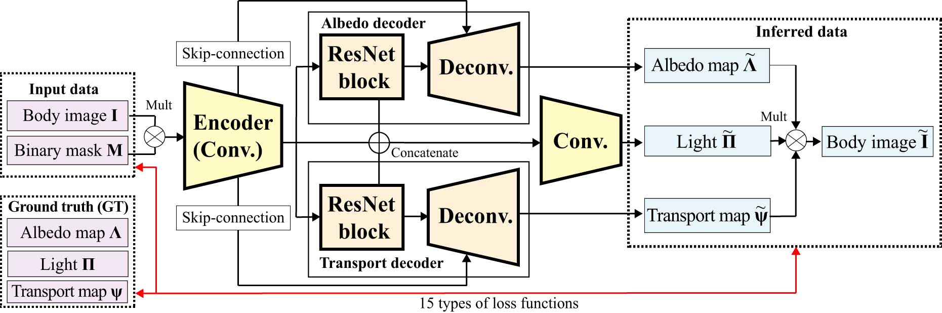
Figure 2. Our network architecture. The input image (multiplied with the binary mask) is fed to the encoder, and the output feature vector is then fed to the decoders of albedo, light transport, and light (Section 5). We calculate 15 types of loss functions by considering the total variations (TVs) for albedo and light transport maps as well as the combinations of inferred outputs and their ground-truth (GT) (Section 4).

In this section, we define the loss functions to infer albedo and light transport maps using our CNNs based on the SH formulation.

For training and testing, we prepare a synthetic human image dataset $\mathcal{D}_{H}$ and an illumination dataset $\mathcal{D}_{L}$ (see Section 6 for the details). The synthetic human image dataset $\mathcal{D}_{H}$ contains a set of a binary mask $\mathbf{M}^{c}_{j}\in\{0,1\}^{N\times c}$ (where $N$ is the number of pixels, $c$ is the number of channels, and $j=1,2,\dots,|\mathcal{D}_{H}|$), albedo map $\mathbf{\Lambda}_{j}\in\mathbb{R}^{N\times 3}$, and light transport map $\mathbf{\Psi}_{j}\in\mathbb{R}^{N\times 9}$ for each 3D human model. The illumination dataset $\mathcal{D}_{L}$ contains SH illumination coefficients for RGB channels $\mathbf{\Pi}_{k}\in\mathbb{R}^{9\times 3}$, where $k=1,2,\dots,|\mathcal{D}_{L}|$. Note that we multiply the binary mask $\mathbf{M}^{c}_{j}$ to the ground-truth data and network outputs (e.g., $\mathbf{M}^{3}_{j}*\mathbf{\Lambda}_{j}$ or $\mathbf{M}^{9}_{j}*\mathbf{\Psi}_{j}$, where $*$ denotes element-wise multiplication) so that we can ignore out-of-mask pixels. In the following explanation, we omit the element-wise multiplication of the binary mask for simplicity.

We use a CNN architecture for inferring light, albedo, and light transport maps (see Section 5 for the network models). The input of the CNN is a masked, RGB full-body human image $\mathbf{I}_{j,k}=\mathbf{\Lambda}_{j}*(\mathbf{\Psi}_{j}\,\mathbf{\Pi}_{k})$. Let $\tilde{\mathbf{\Lambda}}_{j,k}=\tilde{\mathbf{\Lambda}}(\mathbf{I}_{j,k};\Theta_{\lambda})\in\mathbb{R}^{N\times 3}$ be the CNN output for an albedo map, $\tilde{\mathbf{\Psi}}_{j,k}=\tilde{\mathbf{\Psi}}(\mathbf{I}_{j,k};\Theta_{\psi})\in\mathbb{R}^{N\times 9}$ the CNN output for a light transport map, and $\tilde{\mathbf{\Pi}}_{j,k}=\tilde{\mathbf{\Pi}}(\mathbf{I}_{j,k};\Theta_{\pi})\in\mathbb{R}^{N\times 9}$ the CNN output for illumination. Regarding notations, we use tildes ($\,\tilde{}\,$) to indicate inferred outputs, and denote $\tilde{f}(x;y)$ to indicate that $x$ is the input and $y$ is the parameter of network $\tilde{f}$. We optimize these network parameters $\Theta_{\lambda}$, $\Theta_{\psi}$, and $\Theta_{\pi}$ via regression.

Our CNN architecture has a similar design to SfSNet [Sengupta et al., 2018], which infers light, albedo, and normal maps for faces simultaneously. The loss functions used in SfSNet are L1 losses for the inferred albedo map, normal map (from which a light transport map without light occlusion can be calculated analytically), light, and the reconstructed image using the three components. We also use similar four loss functions, but we do not infer normal maps but infer light transport maps directly. Namely, we use L1 losses for $\tilde{\mathbf{\Lambda}}_{j,k}$, $\tilde{\mathbf{\Psi}}_{j,k}$, $\tilde{\mathbf{\Pi}}_{j,k}$, and the reconstructed image $\tilde{\mathbf{I}}_{j,k}=\tilde{\mathbf{\Lambda}}_{j,k}*(\tilde{\mathbf{\Psi}}_{j,k}\,\tilde{\mathbf{\Pi}}_{j,k})$. Furthermore, we also use the following L1 losses:

TV losses::

L1 total variation (TV) losses both for albedo $\tilde{\mathbf{\Lambda}}_{j,k}$ and light transport maps $\tilde{\mathbf{\Psi}}_{j,k}$,

Shading losses::

Three patterns of combination of inferred/GT data to compute a shading map, i.e., $\tilde{\mathbf{\Psi}}_{j,k}\,\mathbf{\Pi}_{k}$, $\mathbf{\Psi}_{j}\,\tilde{\mathbf{\Pi}}_{j,k}$, and $\tilde{\mathbf{\Psi}}_{j,k}\,\tilde{\mathbf{\Pi}}_{j,k}$,

Reconstruction losses::

Six patterns of combination to reconstruct an input image, i.e., $\mathbf{\Lambda}_{j}*(\mathbf{\Psi}_{j}\,\tilde{\mathbf{\Pi}}_{j,k})$, $\mathbf{\Lambda}_{j}*(\tilde{\mathbf{\Psi}}_{j,k}\,\mathbf{\Pi}_{k})$, $\mathbf{\Lambda}_{j}*(\tilde{\mathbf{\Psi}}_{j,k}\,\tilde{\mathbf{\Pi}}_{j,k})$, $\tilde{\mathbf{\Lambda}}_{j,k}*(\mathbf{\Psi}_{j}\,\mathbf{\Pi}_{k})$, $\tilde{\mathbf{\Lambda}}_{j,k}*(\mathbf{\Psi}_{j}\,\tilde{\mathbf{\Pi}}_{j,k})$, and $\tilde{\mathbf{\Lambda}}_{j,k}*(\tilde{\mathbf{\Psi}}_{j,k}\,\mathbf{\Pi}_{k})$.

In total, we use 15 L1 losses. All weights are set to one.

To consider the benefit of the 15 losses, let us take the shading losses, i.e., the three losses for a shading map, as an example. For the multiplication of a light transport map and a light, there are three combinations, namely, GT * inferred (i.e., $\mathbf{\Psi}_{j}\,\tilde{\mathbf{\Pi}}_{j,k}$), inferred * GT (i.e., $\tilde{\mathbf{\Psi}}_{j,k}\,\mathbf{\Pi}_{k}$), and inferred * inferred (i.e., $\tilde{\mathbf{\Psi}}_{j,k}\,\tilde{\mathbf{\Pi}}_{j,k}$), where GT means ground truth. If GT is involved, GT works as a weighting matrix for the inferred output, which enforces the output to lie on a solution manifold in the high-dimensional space. If both are inferred outputs, the loss becomes a soft constraint for the intermediate output, i.e., the inferred shading map. For the choice of loss functions, we chose formulae that do not introduce bias, except for the TV losses. In this way, involving as many formulae that do not introduce bias as possible as losses is a quite general technique, and would be beneficial to other problems. We show an ablation study with and without these losses in Section 7.1.

5. Network Models

Figure 2 illustrates our encoder-decoder network. As mentioned, our network is similar to that of SfSNet, except that ours has much more parameters. Our encoder has six convolutional layers whose output channels are { 64, 128, 256, 512, 512, 512 } and the stride is two. The encoded features are then fed to the decoders for albedo, light transport, and light. The decoders for albedo and light transport maps have almost the same architecture, except that the numbers of output channels are different (i.e., nine for light transport and three for albedo). Each decoder has a residual block (consisting of two convolutional layers with 512 channels) and six deconvolutional layers (output channels are { 512, 512, 256, 128, 64, 9 or 3 } and the stride is also two). The encoder and decoders are connected using skip-connections. For the light decoder, the outputs of the encoder and decoders for albedo and light transport are concatenated and fed to four convolutional layers, which yield a 27-dimensional vector. While SfSNet uses average pooling layers, ours consists of (de-)convolutional layers only. Each (de-)convolutional layer (except for the first and final layers) is followed by batch normalization and (leaky) ReLU. The first three deconvolutional layers of each decoder are followed by dropout with probability 0.5.

6. Dataset Generation

As explained in Section 4, we prepared a synthetic human image dataset and an illumination dataset. Here we explain the details.

Synthetic human image dataset.

Our synthetic human image dataset consists of a binary mask, albedo map, normal map, and light transport map, created by rendering each scanned 3D human figure using a hardware-accelerated renderer. The scanned 3D human figures were obtained from two resources; one is the publicly-available BUFF dataset [Zhang et al., 2017], and the other is commercial websites. The BUFF dataset contains 9,613 standing 3D figures, but lacks variations for our purpose. Namely, it only includes five individuals with one or two outfits each and time-varying poses, and thus subsequent 3D models of the same individual in the same outfit are almost identical. To avoid biasing the training dataset, we manually picked 74 representative models from the BUFF dataset. The commercial data were purchased from different websites and amount to 271 models. We randomly split the models, 345 in total, into 276 training data and 69 test data. Figure 3 shows some examples of our training data. Note that some albedo maps contain self-shadows because shading was not completely removed during the scanning process.

When creating the dataset, we carefully aligned 3D models so that our CNNs can exploit the geometric regularity of our small dataset. Namely, we rendered front-facing figures in the middle of square images while aligning them so that they have almost the same vertical size in the images with vertical paddings at the top and bottom of a fixed size (5% of image heights). Regarding poses, we only used standing figures and removed sitting ones from our training/test datasets. The image resolution is $1024\times 1024$ pixels. No data augmentation is employed for the human image dataset.

Illumination dataset.

For our illumination dataset, we used the Laval Indoor HDR dataset [Gardner et al., 2017] containing 2,144 environment maps in panoramic HDR format. We first converted them into diffuse SH coefficients and calculated a reference brightness of each environment map using Equation (5) with a front-facing normal $\mathbf{n}=(0,0,1)^{T}$. We omitted dark environment maps if the reference brightness is lower than 0.2, and scaled the brightness of other environment maps so that reference brightness lies within $[0.7,0.9]$. To obtain further variations, we rotated each data 35 times by 10 degrees around the vertical axis. We then reduced the redundancy using k-means clustering and manually removed unusual illuminations (e.g., too bright lights, back-lights, and lights causing too strong contrasts in shadings). Finally, from the remaining 50 illuminations, we randomly picked 40 illuminations for training and 10 for testing. Figure 4 shows some examples of our training data.

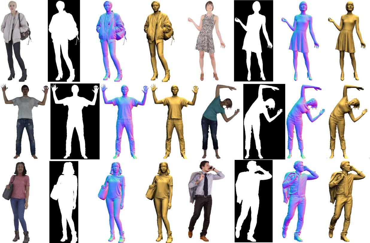
Figure 3. Examples from our synthetic human image dataset. For each human figure, an albedo map, binary mask, normal map, and light transport map (visualized as a shading map) are displayed. Note that some albedo maps contain self-shadows due to scanning inadequacy. Each image is trimmed.

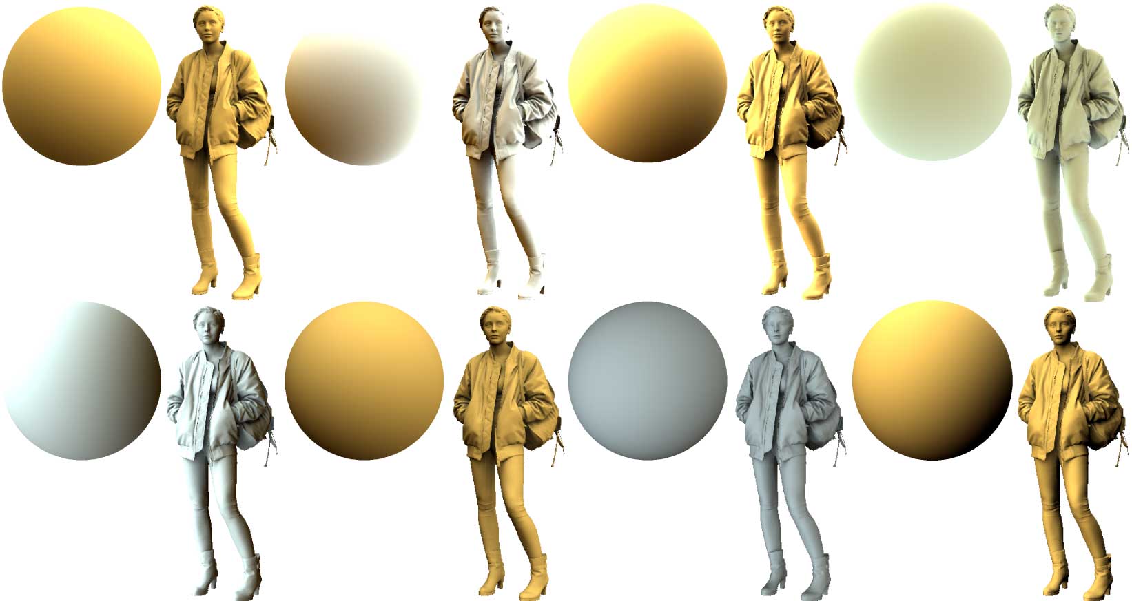
Figure 4. Examples from our illumination dataset. SH illumination coefficients are visualized as shading maps of a sphere and the top-left model in Figure 3.

7. Experiments

Table 1. RMSE and SSIM for the inferred results using each method. The light transport maps of SfSNet and SfSNet-AO were computed from corresponding normal maps analytically. Best values are highlighted in boldface.

	RMSE within binary masks						SSIM within bounding boxes of masks
	Shading	Transport	Normal	AO	Light	Albedo	Shading	Transport	Normal	AO	Light	Albedo
SfSNet	0.299	0.526	0.346	N/A	0.207	0.135	0.884	0.755	0.776	N/A	0.446	0.954
SfSNet-AO	0.293	0.529	0.347	0.083	0.207	0.131	0.890	0.749	0.772	0.946	0.475	0.955
Ours (min)	0.237	0.406	N/A	N/A	0.205	0.131	0.909	0.777	N/A	N/A	0.473	0.953
Ours (full)	0.219	0.393	N/A	N/A	0.199	0.129	0.927	0.781	N/A	N/A	0.500	0.943

Table 2. RMSE and SSIM for an ablation study for our 15-losses. Best values are highlighted in boldface.

	RMSE				SSIM
	Shading	Transport	Light	Albedo	Shading	Transport	Light	Albedo
W/o TV	0.226	0.391	0.202	0.126	0.923	0.784	0.471	0.956
W/o shading	0.227	0.398	0.201	0.132	0.922	0.781	0.496	0.940
W/o reconstruction	0.224	0.394	0.198	0.144	0.925	0.782	0.503	0.907

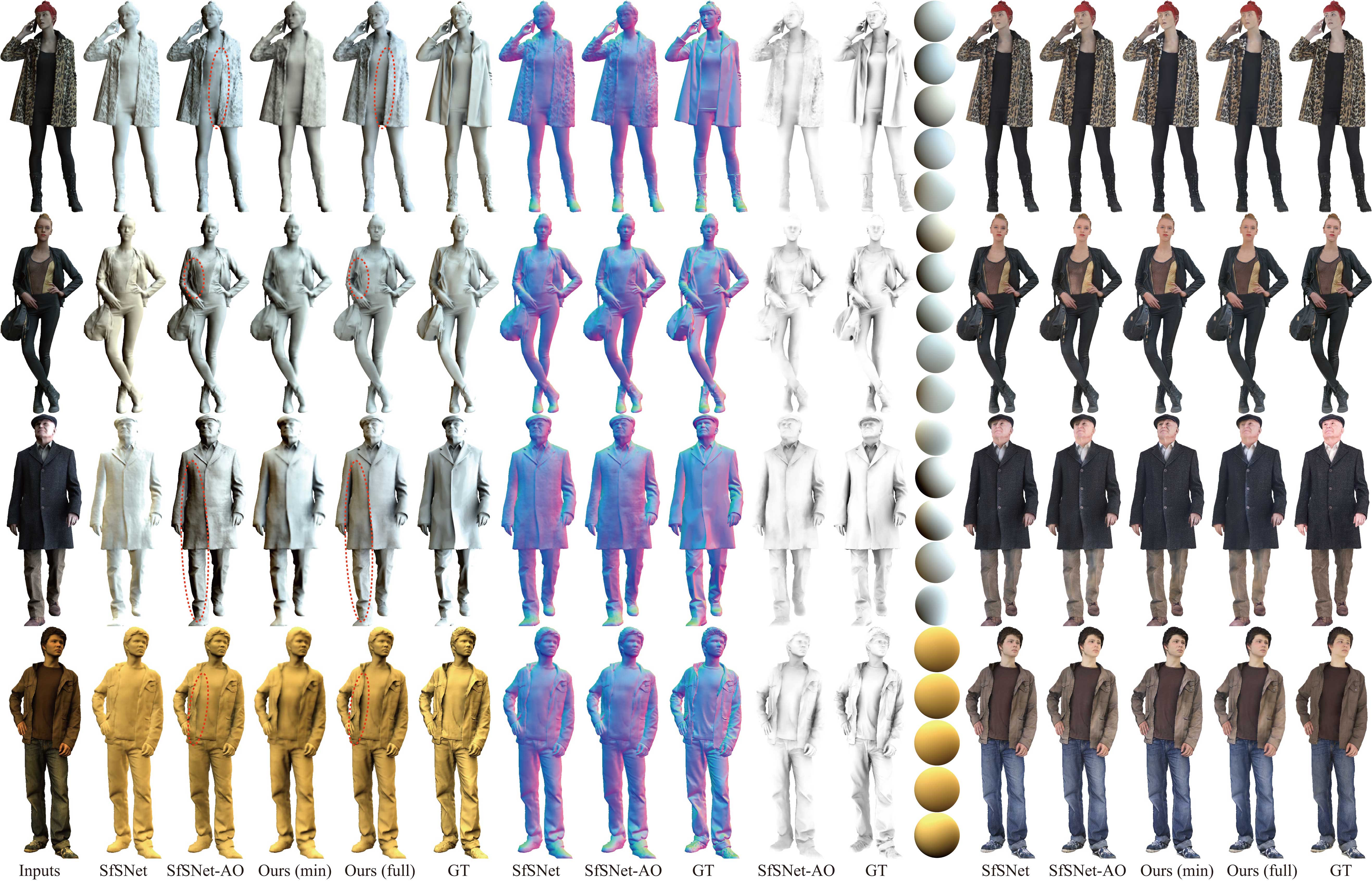
Figure 5. Comparisons with synthetic data. From left to right, input images, shading maps, normal maps, ambient occlusion maps, light maps (i.e., light information visualized by shading a sphere), and albedo maps. The light maps are in the same order as shading/albedo maps, from top to bottom. The red ovals in inferred shading maps highlight differences between SfSNet-AO and “Ours (full).”

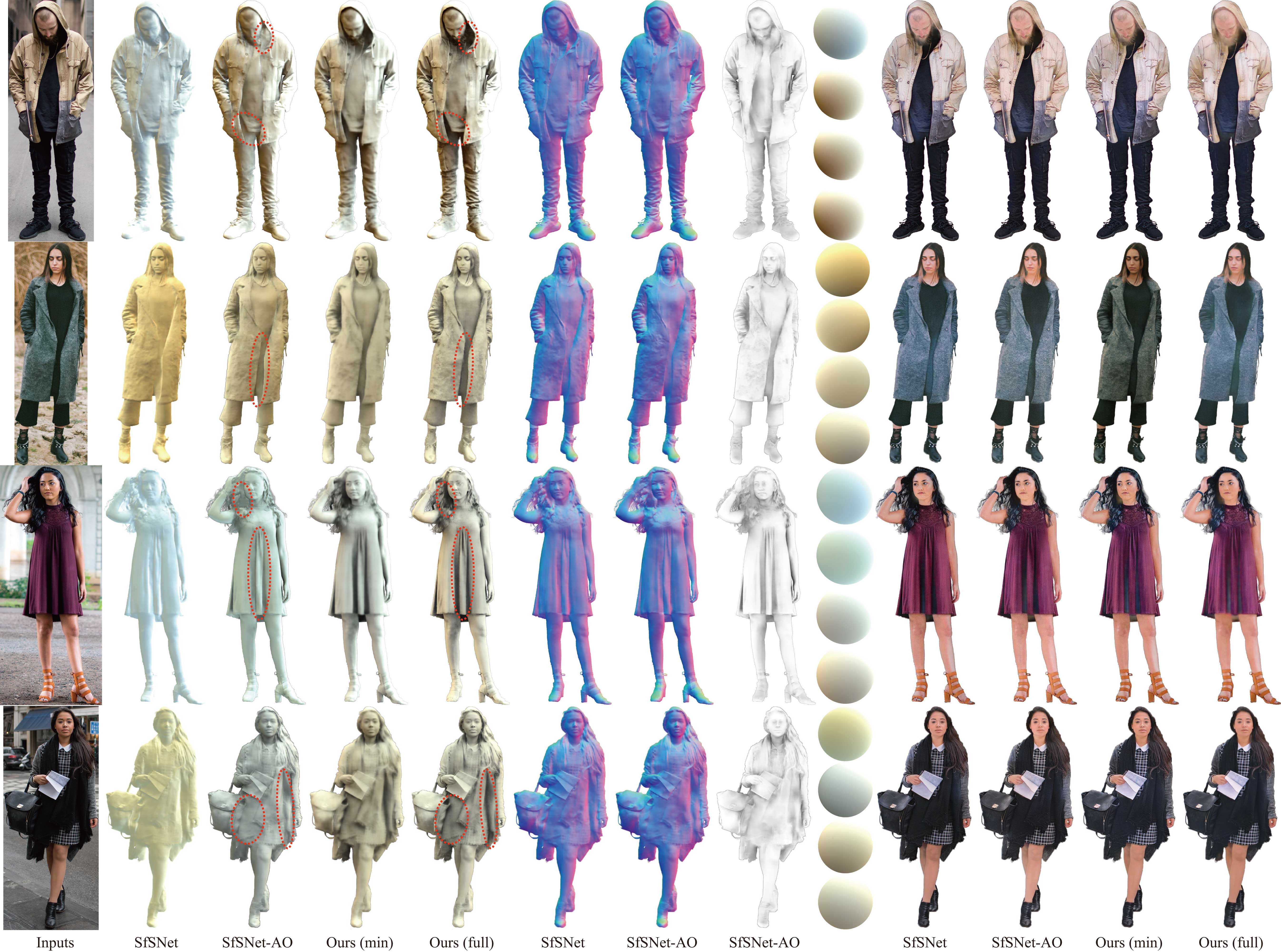
Figure 6. Comparisons with real photographs. The red ovals in inferred shading maps highlight differences between SfSNet-AO and “Ours (full).” Input images courtesy of Guillaume Bolduc, George Gvasalia, Jacob Postuma, and Kat Garcia.

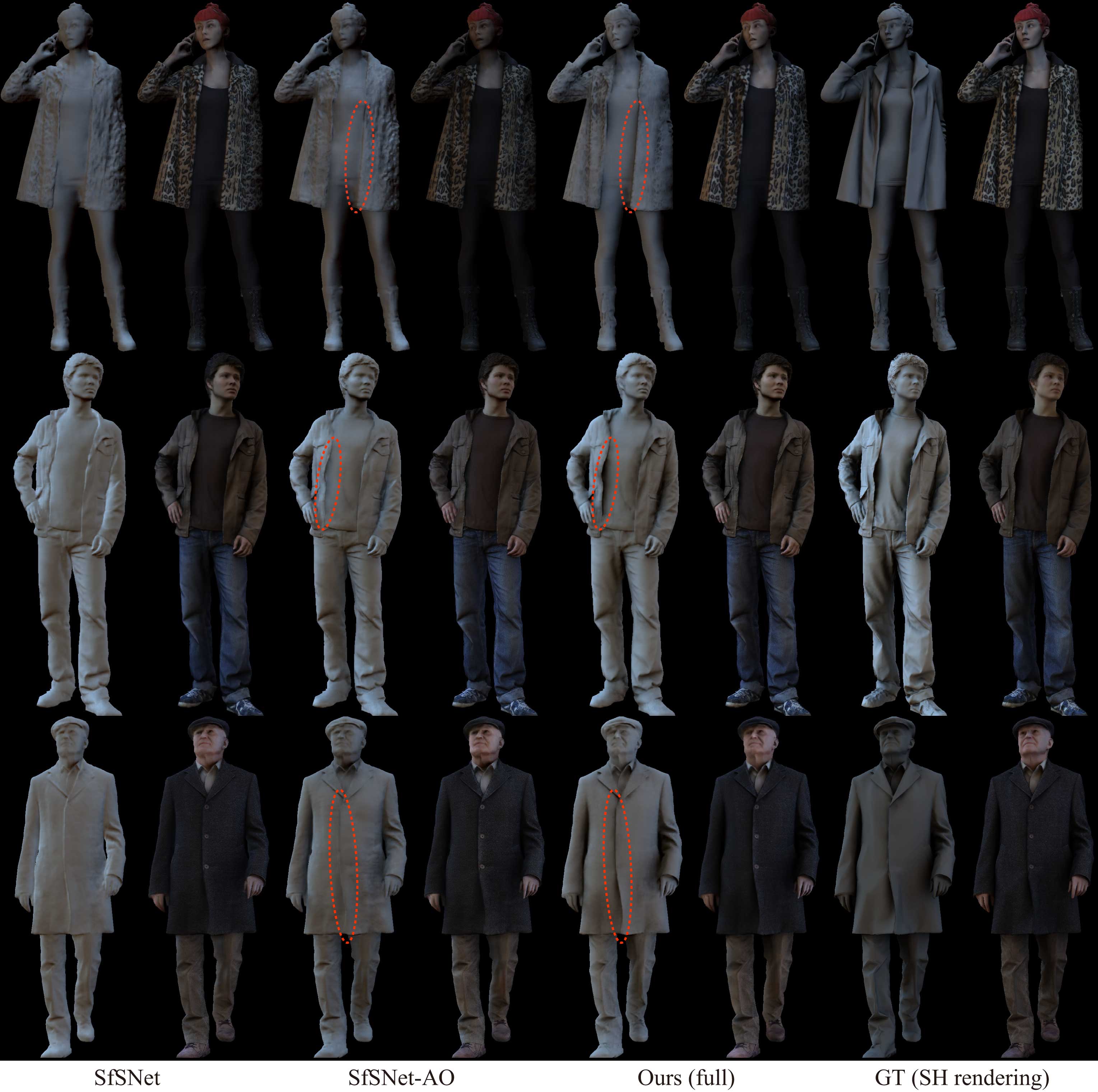
Figure 7. Relighting comparison using synthetic data. The red ovals highlight differences between SfSNet-AO and “Ours (full).”

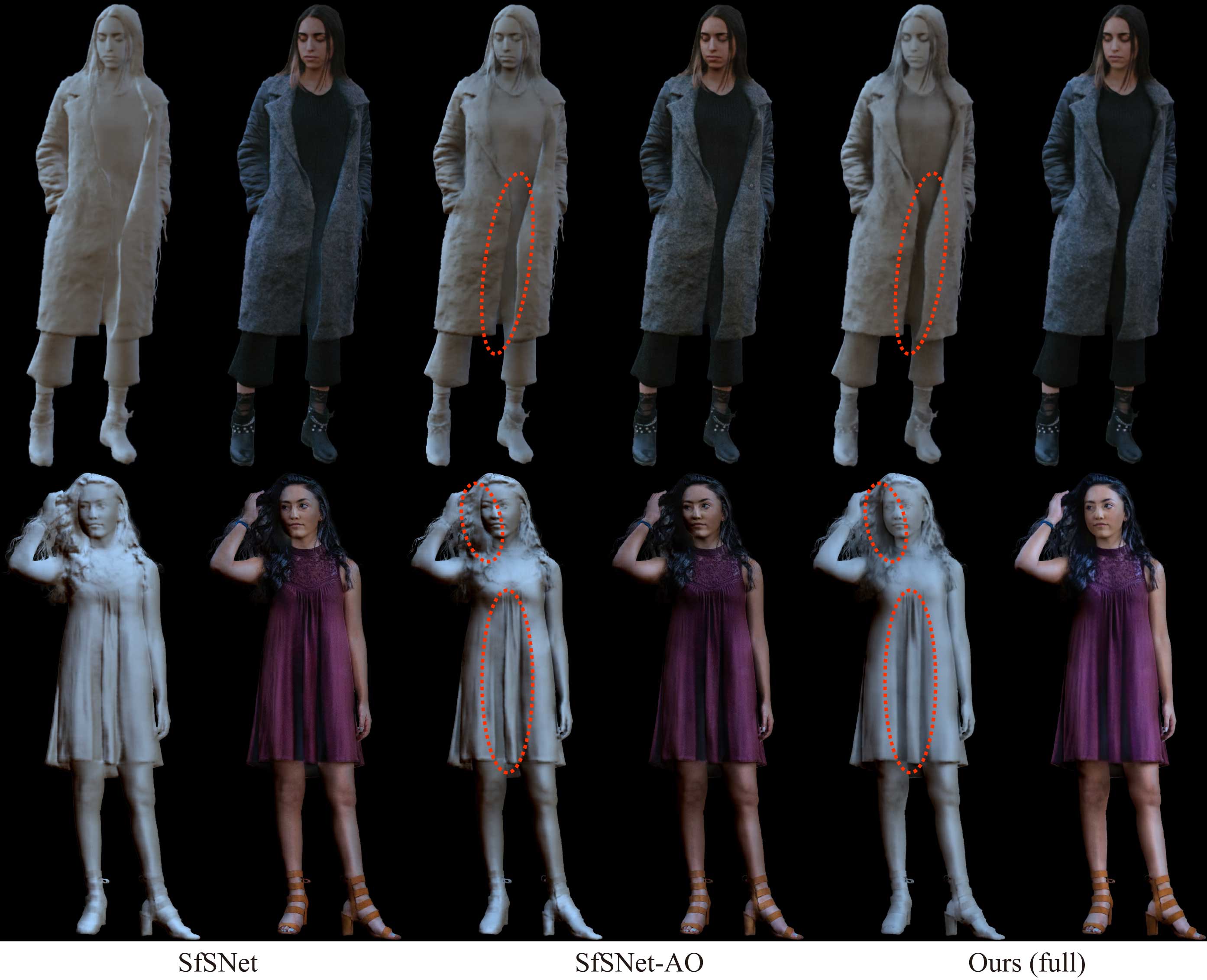
Figure 8. Relighting comparison using real photographs. The red ovals highlight differences between SfSNet-AO and “Ours (full).” Input images courtesy of George Gvasalia and Jacob Postuma.

We implemented our CNN models using Python and the chainer library, and ran our code on a PC with NVIDIA GeForce GTX 1080 Ti GPUs. We used Adam as an optimizer with a fixed learning rate 0.0002 and batch size 1. The computation times for one epoch of training on a single GPU were about three hours with our CNN models. We used the synthetic images of $1024\times 1024$ pixels for training in our results. Our CNN models, as well as other models for comparisons, were trained up to 60 epochs. For relighting, we used Debevec’s environment maps [2004], namely, kitchen_probe for Figures 1, 7, and 8 and grace_probe for Figure 1. The input photographs in our results were downloaded from Unsplash. Specifically, we selected high-quality free-license images of single human figures, generated their binary masks automatically using Adobe Photoshop with manual correction, applied trimming and uniform scaling, and then added paddings to make them $1024\times 1024$ pixels.

7.1. Comparisons of Inference

To clarify the advantage of our method, we compared it with three alternative methods. The first one is SfSNet [Sengupta et al., 2018], but the network architecture is not the original one for small $128\times 128$ images but much richer one defined in Section 5. In this case, a decoder of SfSNet outputs three-channel normal maps, instead of nine-channel light transport maps. The second method is SfSNet plus ambient occlusion (hereafter we call it SfSNet-AO). A single-channel ambient occlusion is inferred by an additional decoder branch. The third method is our network with four losses only, similar to SfSNet. We refer to the 4-loss version as “Ours (min)” and the 15-loss version as “Ours (full).” Comparisons between “SfSNet” and “Ours (min)” reveal the impact of considering light occlusion whereas those between “Ours (min)” and “Ours (full)” demonstrate the effectiveness of the full loss.

Figures 5 and 6 show the results of qualitative comparisons using synthetic test data and photographs, respectively. The red ovals in inferred shading maps highlight differences between SfSNet-AO and “Ours (full).” The first row of Figure 5 indicates that all methods suffer from separating textures from shading maps. The shading maps of SfSNet often seem like flat bas-reliefs because light occlusion is ignored. In the first and fourth rows, SfSNet-AO estimates the depth gaps between jackets and shirts smaller than the actual gap. Such biased estimate in shading maps often yields unnaturally-darkened albedo maps. Comparing our two variants, i.e., “Ours (min)” and “Ours (full)”, the latter yields sharper shading maps than the former. Also in Figure 6, we can see the similar tendency with real photographs.

For quantitative comparison, Table 1 summarizes the RMSE and SSIM of each component. To reduce the effects of out-of-mask-pixels, we calculate RMSEs within binary masks whereas we calculate SSIMs within the bounding boxes of binary masks. The table shows that “Ours (full)” is consistently better than other alternatives except for “Albedo SSIM”. The reason why “Albedo SSIM” of “Ours (full)” is lower than others is that “Ours(full)” better cancels the baked-in shadings (see Section 6) in GT albedos and thus its output albedos become more dissimilar to “GT.” Table 2 further reveals the impacts of the TV losses, shading losses, and reconstruction losses. We can see the tendency that overall the accuracies are lower than those of “Ours (full)” in Table 1. Note that light transport and albedo maps of “W/o TV” are slightly better than those of “Ours (full).” This result is reasonable because TV losses enforce smoothing, i.e., add biases, to the inferred outputs in compensation for generalization capability.

7.2. Relighting and Light Transfer

Figures 7 and 8 show the results of relighting with inferred albedo and light transport maps, given synthetic test images and real photographs, respectively. Comparisons with path-traced reference images as well as movies are available in the supplemental material.

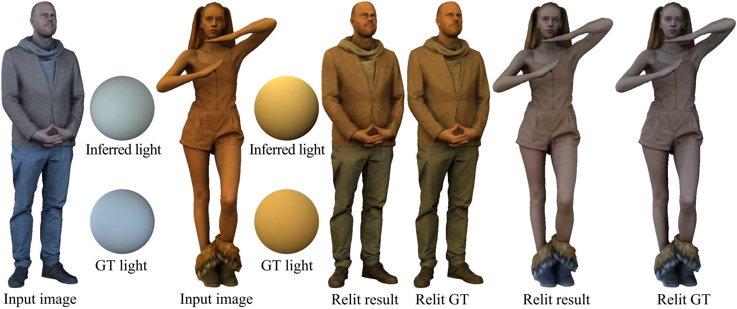
Figure 9. Light transfer. By performing inference for two images and swapping inferred lights, we can transfer the inferred light to each other.

By inferring illuminations in two human portraits, we can transfer the inferred illumination to each other. Figure 9 shows the results of light transfer with synthetic human images. The inferred illuminations have colors slightly different from the ground-truth, but the patterns of the illuminations are similar. The relit human images are therefore similar to the ground-truth.

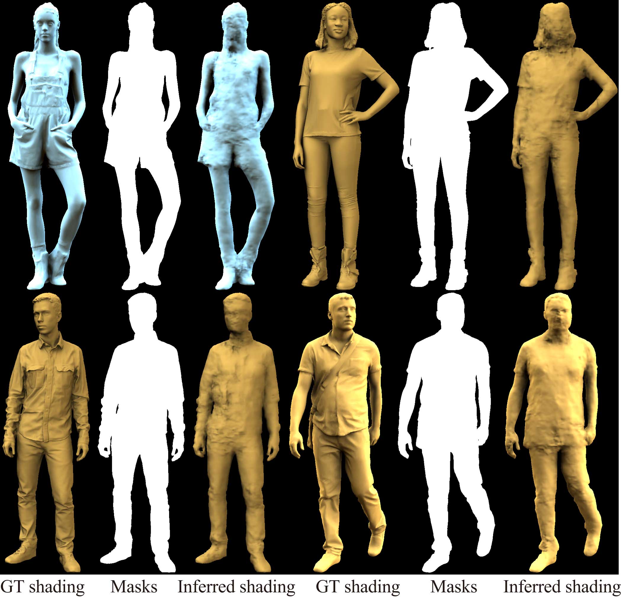
Figure 10. Shape from mask. For each human figure, a ground-truth shading map, mask, and inferred shading map are displayed. These results imply that our network can learn a strong shape prior from silhouettes.

8. Discussions

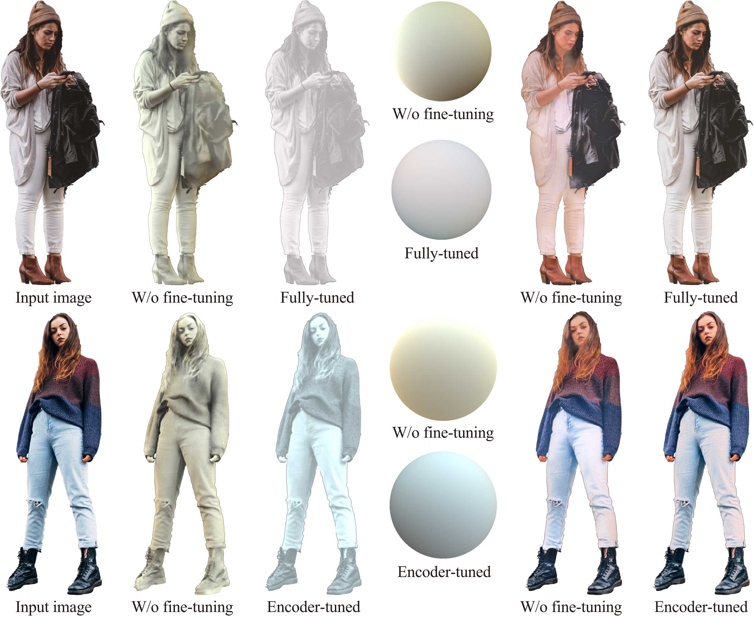
Figure 11. Comparison to self-supervised learning. By fine-tuning network parameters using only unlabeled photographs with (i.e., encoder-tuned; lower row) and without (i.e., fully-tuned; upper row) fixing decoders, the outputs collapsed; the shading maps bleached and the albedo maps got close to the input images. Input images courtesy of Philip Martin and Ali Morshedlou.

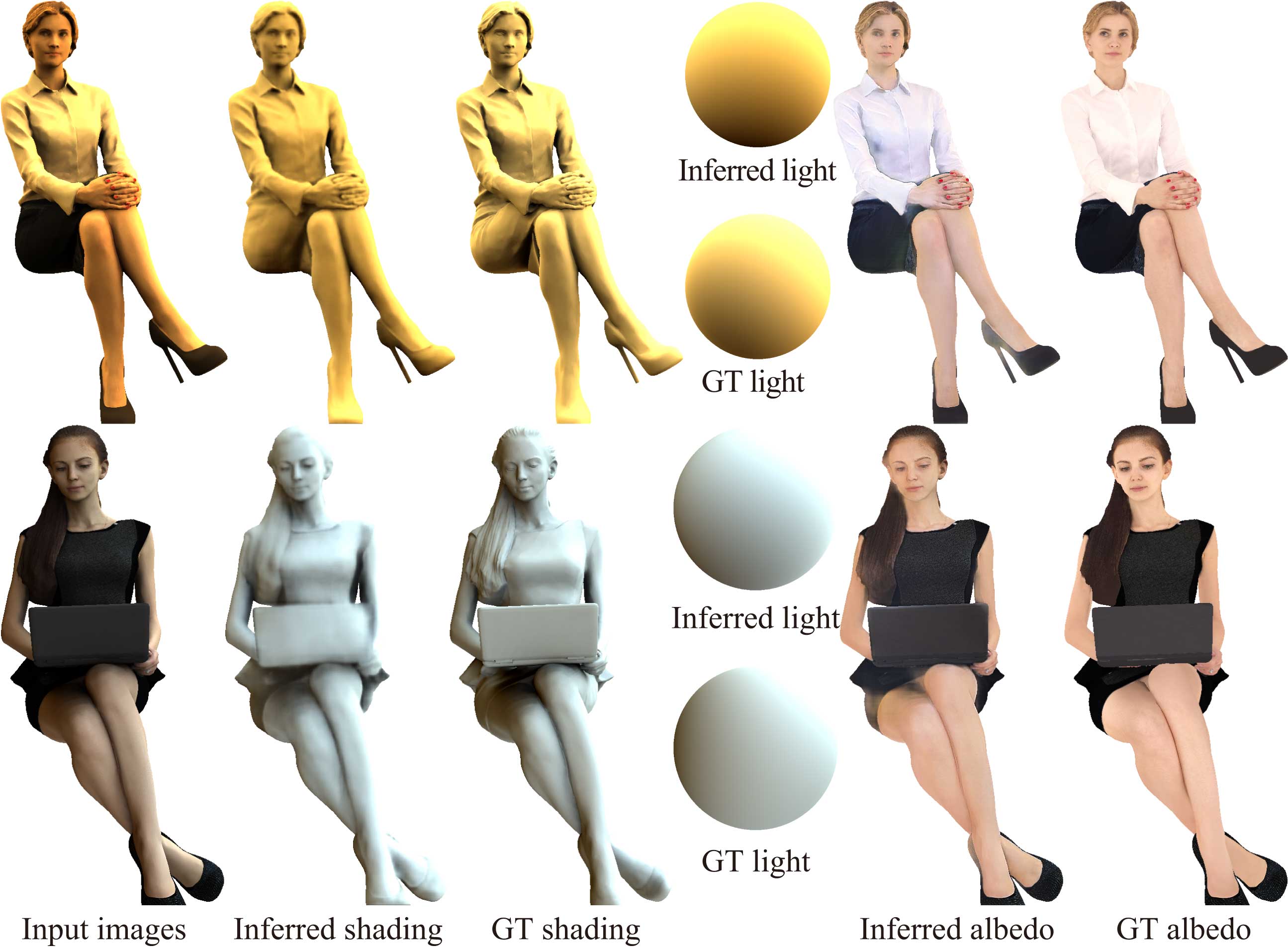
Figure 12. Inferred results with sitting poses. Our network can handle sitting poses unexpectedly well even though it is not trained with them.

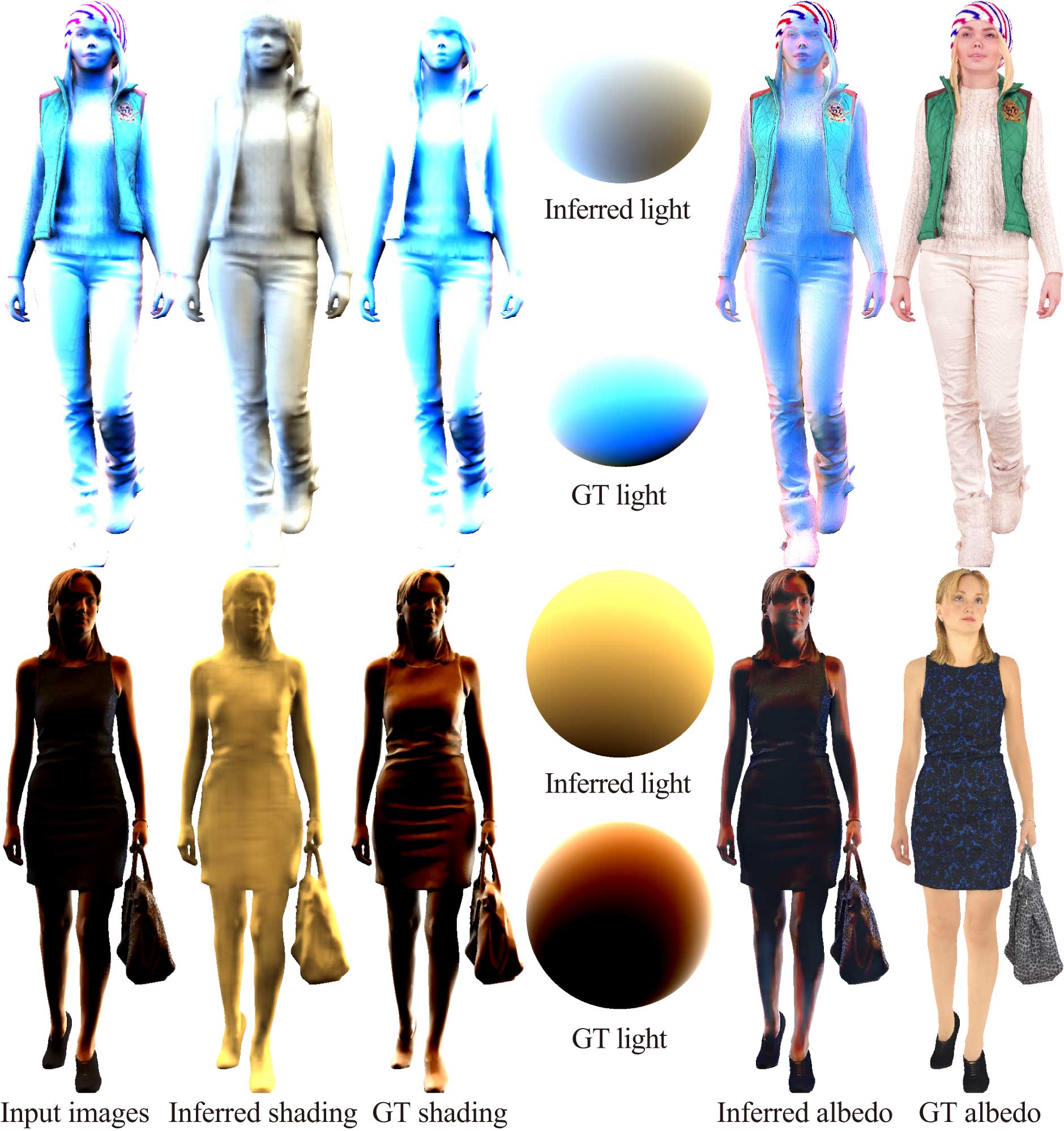
Figure 13. Failure examples with unusual lights. Our network suffers from inferring lights quite different from the training data.

Silhouettes as priors.

Some existing methods [Barron and Malik, 2015; Lun et al., 2017] on shape-from-shading suggested that object silhouettes serve as shape priors. In the recent work of the CNN-based shape inference from 2D silhouettes [Lun et al., 2017], the size of the training dataset is around ten thousand. Compared to this size, it was a surprise that we can infer plausible albedo and shading from only a few hundreds of training data. To confirm how much the silhouettes help our inference, we inferred light transport maps only from the binary masks. For this inference, we used the CNN model for light transport maps and used only those loss functions related to light transport maps. Figure 10 shows the resultant shading maps and corresponding ground-truth. Surprisingly, we can observe the rough concave shapes under the chin and the flat shapes of the instep. This result implies that our CNN models also learned a strong shape prior from silhouettes thanks to the regularity of our small training dataset.

Self-supervised learning.

Recent methods for intrinsic decomposition or image disentanglement, e.g., [Sengupta et al., 2018], often employ self-supervised learning to fine-tune networks that are trained with synthetic data; only the single loss for the differences between input images and products of inferred outputs is considered, and the network is trained using unlabeled real photographs. We fine-tuned the model of “Ours (full)” with and without fixing the network parameters of the decoders. However, in both cases, the inferred outputs collapsed (see Figure 11); the light transport maps lost details, the corresponding shading maps bleached, and the albedo maps got close to the input images. This is probably because our light transport maps have much larger degrees of freedom (i.e., nine dimensions per pixel) than normal maps inferred in [Sengupta et al., 2018], and thus are more difficult to fine-tune under the unconstrained setting in self-supervised learning. We thus did not adopt self-supervised learning in other results. The details of the experimental settings are available in the supplemental material.

Sitting poses.

To evaluate the ability of our network for handling various poses, we fed synthetic human images in sitting poses, which were not included in training or test data. Figure 12 shows the results. The inferred outputs are unexpectedly well compared to the ground-truth, which is probably because our training dataset is sufficiently rich for the network to learn shapes of body parts such as arms and legs.

Unusual lights.

We also evaluated the ability for handling various lights, as shown in Figure 13. Unfortunately, our network could not plausibly infer lights that were quite different from those in our training data. Our network seems to reconstruct nearest-neighbor lights that can be found in the training dataset, and the light transport maps are inferred accordingly. The large differences in appearance are then encoded in the inferred albedo maps so that the products of the three components become similar to the input images. A straightforward solution is to enrich the training light dataset using, e.g., the environment maps used in [Endo et al., 2017], so that good nearest neighbors can be found for various inputs.

8.1. Limitations

Here we explain the limitations of our method. Although our method is based on a better formulation of SH-based lighting, i.e., with consideration of light occlusion, it is still a crude approximation of lighting calculation. First of all, we only handle diffuse albedo. This limitation mainly stems from our dataset; most of the commercial data do not have specular components, even though SH representation can naturally handle specular components as demonstrated in the original PRT paper. Adding artificial specular components to our training dataset, as done in [Innamorati et al., 2017], seems inappropriate in our case because human skin and clothes should have different reflectance. Material assignment with semantic segmentation for hundreds of meshes is ideal but can be a challenging project by itself. As our work is the first attempt regarding both full-body relighting and SH-based light occlusion learning/inference, we believe this limitation is acceptable to encourage follow-up studies.

Also, while we used second-order SH for representing light occlusion, Sloan et al. [2002] suggested to use higher-order bases because occlusion causes high-frequency signals. As is often the case with learning-based methods, our method might fail with conditions quite dissimilar to the training dataset, e.g., harsh illuminations, as demonstrated in Figure 13.

9. Conclusions and Future Work

In this paper, we have paved the way to occlusion-aware relighting from single-view human images and accompanying inference using CNNs. Inspired by the seminal work of the precomputed radiance transfer [Sloan et al., 2002], we employed SH-based lighting, i.e., dot-product calculation of second-order spherical harmonics (SH) coefficient vectors of illumination and occlusion (i.e., light transfer vectors), and trained our models using our synthetic ground-truth dataset. Plausible inference of albedo and light transport maps were possible probably because of our small yet geometrically-aligned human image dataset. By considering light occlusion, inferred albedo and shading maps (i.e., the product of a light transport map and illumination) as well as relighting results are more plausible than those obtained by using previous techniques without considering light occlusion.

One obvious direction of future work is to extend our first attempt to more physically-accurate inverse rendering, based on the formulations extensively studied in the literature of precomputed radiance transfer. For example, other basis functions such as wavelets or spherical Gaussians might be beneficial to handle high-frequency shadows or illumination. A quite important future work would be to build a publicly-available, high-quality 3D human models, which is crucial to develop this human-oriented research.

- [1]
- Aittala et al. [2016] Miika Aittala, Timo Aila, and Jaakko Lehtinen. 2016. Reflectance modeling by neural texture synthesis. ACM Trans. Graph. 35, 4 (2016), 65:1–65:13.
- Anguelov et al. [2005] Dragomir Anguelov, Praveen Srinivasan, Daphne Koller, Sebastian Thrun, Jim Rodgers, and James Davis. 2005. SCAPE: shape completion and animation of people. ACM Trans. Graph. 24, 3 (2005), 408–416.
- Balan et al. [2007] Alexandru O. Balan, Leonid Sigal, Michael J. Black, James E. Davis, and Horst W. Haussecker. 2007. Detailed Human Shape and Pose from Images. In 2007 IEEE Computer Society Conference on Computer Vision and Pattern Recognition (CVPR 2007).
- Barron and Malik [2015] Jonathan T. Barron and Jitendra Malik. 2015. Shape, Illumination, and Reflectance from Shading. IEEE Trans. Pattern Anal. Mach. Intell. 37, 8 (2015), 1670–1687.
- Barrow and Tenenbaum [1978] H. G. Barrow and J. M. Tenenbaum. 1978. Recovering intrinsic scene characteristics from images. Comp. Vis. Sys. (1978).
- Baslamisli et al. [2018] Anil S. Baslamisli, Hoang-An Le, and Theo Gevers. 2018. CNN based Learning using Reflection and Retinex Models for Intrinsic Image Decomposition. In Proceedings of the IEEE Conference on Computer Vision and Pattern Recognition (CVPR 2018).
- Basri and Jacobs [2003] R. Basri and D. W. Jacobs. 2003. Lambertian reflectance and linear subspaces. IEEE Transactions on Pattern Analysis and Machine Intelligence 25, 2 (Feb 2003), 218–233.
- Bell et al. [2014] Sean Bell, Kavita Bala, and Noah Snavely. 2014. Intrinsic images in the wild. ACM Trans. Graph. 33, 4 (2014), 159:1–159:12.
- Blanz and Vetter [1999] Volker Blanz and Thomas Vetter. 1999. A Morphable Model for the Synthesis of 3D Faces. In Proceedings of the 26th Annual Conference on Computer Graphics and Interactive Techniques (SIGGRAPH 1999). 187–194.
- Bonneel et al. [2017] Nicolas Bonneel, Balazs Kovacs, Sylvain Paris, and Kavita Bala. 2017. Intrinsic Decompositions for Image Editing. Comput. Graph. Forum 36, 2 (2017), 593–609.
- Chai et al. [2015] Menglei Chai, Linjie Luo, Kalyan Sunkavalli, Nathan Carr, Sunil Hadap, and Kun Zhou. 2015. High-quality hair modeling from a single portrait photo. ACM Trans. Graph. 34, 6 (2015), 204:1–204:10.
- Chandraker and Ramamoorthi [2011] Manmohan Krishna Chandraker and Ravi Ramamoorthi. 2011. What an image reveals about material reflectance. In IEEE International Conference on Computer Vision (ICCV 2011). 1076–1083.
- Danerek et al. [2017] R. Danerek, Endri Dibra, A. Cengiz Öztireli, Remo Ziegler, and Markus H. Gross. 2017. DeepGarment: 3D Garment Shape Estimation from a Single Image. Comput. Graph. Forum 36, 2 (2017), 269–280.
- Debevec [2004] Paul Debevec. 2004. Light Probe Image Gallery. http://www.pauldebevec.com/Probes/.
- Debevec et al. [2000] Paul E. Debevec, Tim Hawkins, Chris Tchou, Haarm-Pieter Duiker, Westley Sarokin, and Mark Sagar. 2000. Acquiring the reflectance field of a human face. In Proceedings of the 27th Annual Conference on Computer Graphics and Interactive Techniques (SIGGRAPH 2000). 145–156.
- Endo et al. [2017] Yuki Endo, Yoshihiro Kanamori, and Jun Mitani. 2017. Deep reverse tone mapping. ACM Trans. Graph. 36, 6 (2017), 177:1–177:10.
- Gardner et al. [2017] Marc-André Gardner, Kalyan Sunkavalli, Ersin Yumer, Xiaohui Shen, Emiliano Gambaretto, Christian Gagné, and Jean-François Lalonde. 2017. Learning to predict indoor illumination from a single image. ACM Trans. Graph. 36, 6 (2017), 176:1–176:14.
- Garrido et al. [2013] Pablo Garrido, Levi Valgaerts, Chenglei Wu, and Christian Theobalt. 2013. Reconstructing detailed dynamic face geometry from monocular video. ACM Trans. Graph. 32, 6 (2013), 158:1–158:10.
- Georgoulis et al. [2018] Stamatios Georgoulis, Konstantinos Rematas, Tobias Ritschel, Efstratios Gavves, Mario Fritz, Luc Van Gool, and Tinne Tuytelaars. 2018. Reflectance and Natural Illumination from Single-Material Specular Objects Using Deep Learning. IEEE Trans. Pattern Anal. Mach. Intell. 40, 8 (2018), 1932–1947.
- Guan et al. [2009] Peng Guan, Alexander Weiss, Alexandru O. Balan, and Michael J. Black. 2009. Estimating human shape and pose from a single image. In IEEE 12th International Conference on Computer Vision (ICCV 2009). 1381–1388.
- Hold-Geoffroy et al. [2017] Yannick Hold-Geoffroy, Kalyan Sunkavalli, Sunil Hadap, Emiliano Gambaretto, and Jean-François Lalonde. 2017. Deep Outdoor Illumination Estimation. In 2017 IEEE Conference on Computer Vision and Pattern Recognition (CVPR 2017). 2373–2382.
- Horn [1989] Berthold K. P. Horn. 1989. Shape from Shading. MIT Press, Chapter Obtaining Shape from Shading Information, 123–171.
- Innamorati et al. [2017] Carlo Innamorati, Tobias Ritschel, Tim Weyrich, and Niloy J. Mitra. 2017. Decomposing Single Images for Layered Photo Retouching. Comput. Graph. Forum 36, 4 (2017), 15–25.
- Johnson and Adelson [2011] Micah K. Johnson and Edward H. Adelson. 2011. Shape estimation in natural illumination. In The 24th IEEE Conference on Computer Vision and Pattern Recognition (CVPR 2011). 2553–2560.
- Kemelmacher-Shlizerman and Basri [2011] Ira Kemelmacher-Shlizerman and Ronen Basri. 2011. 3D Face Reconstruction from a Single Image Using a Single Reference Face Shape. IEEE Trans. Pattern Anal. Mach. Intell. 33, 2 (2011), 394–405.
- Kholgade et al. [2014] Natasha Kholgade, Tomas Simon, Alexei A. Efros, and Yaser Sheikh. 2014. 3D object manipulation in a single photograph using stock 3D models. ACM Trans. Graph. 33, 4 (2014), 127:1–127:12.
- Land and McCann [1971] Edwin H. Land and John J. McCann. 1971. Lightness and Retinex Theory. J. Opt. Soc. Am. 61, 1 (Jan 1971), 1–11.
- Li et al. [2013] Guannan Li, Chenglei Wu, Carsten Stoll, Yebin Liu, Kiran Varanasi, Qionghai Dai, and Christian Theobalt. 2013. Capturing Relightable Human Performances under General Uncontrolled Illumination. Comput. Graph. Forum 32, 2 (2013), 275–284.
- Li et al. [2017] Xiao Li, Yue Dong, Pieter Peers, and Xin Tong. 2017. Modeling surface appearance from a single photograph using self-augmented convolutional neural networks. ACM Trans. Graph. 36, 4 (2017), 45:1–45:11.
- Lopez-Moreno et al. [2013] Jorge Lopez-Moreno, Elena Garces, Sunil Hadap, Erik Reinhard, and Diego Gutierrez. 2013. Multiple Light Source Estimation in a Single Image. Comput. Graph. Forum 32, 8 (2013), 170–182.
- Lun et al. [2017] Zhaoliang Lun, Matheus Gadelha, Evangelos Kalogerakis, Subhransu Maji, and Rui Wang. 2017. 3D Shape Reconstruction from Sketches via Multi-view Convolutional Networks. In 2017 International Conference on 3D Vision (3DV 2017).
- Narihira et al. [2015] Takuya Narihira, Michael Maire, and Stella X. Yu. 2015. Direct Intrinsics: Learning Albedo-Shading Decomposition by Convolutional Regression. In 2015 IEEE International Conference on Computer Vision (ICCV 2015). 2992.
- Oxholm and Nishino [2012] Geoffrey Oxholm and Ko Nishino. 2012. Shape and Reflectance from Natural Illumination. In 12th European Conference on Computer Vision (ECCV 2012), Proceedings, Part I. 528–541.
- Paysan et al. [2009] Pascal Paysan, Reinhard Knothe, Brian Amberg, Sami Romdhani, and Thomas Vetter. 2009. A 3D Face Model for Pose and Illumination Invariant Face Recognition. In Sixth IEEE International Conference on Advanced Video and Signal Based Surveillance (AVSS 2009). 296–301.
- Ramamoorthi and Hanrahan [2001] Ravi Ramamoorthi and Pat Hanrahan. 2001. An efficient representation for irradiance environment maps. In Proceedings of the 28th Annual Conference on Computer Graphics and Interactive Techniques, SIGGRAPH 2001. 497–500.
- Schneider et al. [2017] Andreas Schneider, Sandro Schönborn, Bernhard Egger, Lavrenti Frobeen, and Thomas Vetter. 2017. Efficient Global Illumination for Morphable Models. In IEEE International Conference on Computer Vision (ICCV 2017). 3885–3893.
- Sengupta et al. [2018] Soumyadip Sengupta, Angjoo Kanazawa, Carlos D. Castillo, and David W. Jacobs. 2018. SfSNet: Learning Shape, Reflectance and Illuminance of Faces ‘in the Wild’. In Proceedings of the IEEE Conference on Computer Vision and Pattern Recognition (CVPR 2018).
- Shi et al. [2017] Jian Shi, Yue Dong, Hao Su, and Stella X. Yu. 2017. Learning Non-Lambertian Object Intrinsics Across ShapeNet Categories. In 2017 IEEE Conference on Computer Vision and Pattern Recognition (CVPR 2017). 5844–5853.
- Shu et al. [2017a] Zhixin Shu, Sunil Hadap, Eli Shechtman, Kalyan Sunkavalli, Sylvain Paris, and Dimitris Samaras. 2017a. Portrait Lighting Transfer Using a Mass Transport Approach. ACM Trans. Graph. 36, 4, Article 145a (Oct. 2017).
- Shu et al. [2017b] Zhixin Shu, Ersin Yumer, Sunil Hadap, Kalyan Sunkavalli, Eli Shechtman, and Dimitris Samaras. 2017b. Neural Face Editing with Intrinsic Image Disentangling. In 2017 IEEE Conference on Computer Vision and Pattern Recognition (CVPR 2017). 5444–5453.
- Sloan et al. [2002] Peter-Pike J. Sloan, Jan Kautz, and John Snyder. 2002. Precomputed radiance transfer for real-time rendering in dynamic, low-frequency lighting environments. ACM Trans. Graph. 21, 3 (2002), 527–536.
- Tewari et al. [2017] Ayush Tewari, Michael Zollhöfer, Hyeongwoo Kim, Pablo Garrido, Florian Bernard, Patrick Pérez, and Christian Theobalt. 2017. MoFA: Model-Based Deep Convolutional Face Autoencoder for Unsupervised Monocular Reconstruction. In IEEE International Conference on Computer Vision (ICCV 2017). 3735–3744.
- Xue et al. [2012] Su Xue, Aseem Agarwala, Julie Dorsey, and Holly E. Rushmeier. 2012. Understanding and improving the realism of image composites. ACM Trans. Graph. 31, 4 (2012), 84:1–84:10.
- Yamaguchi et al. [2018] Shugo Yamaguchi, Shunsuke Saito, Koki Nagano, Yajie Zhao, Weikai Chen, Kyle Olszewski, Shigeo Morishima, and Hao Li. 2018. High-fidelity Facial Reflectance and Geometry Inference from an Unconstrained Image. ACM Trans. Graph. 37, 4, Article 162 (July 2018), 162:1–162:14 pages.
- Zhang et al. [2017] Chao Zhang, Sergi Pujades, Michael J. Black, and Gerard Pons-Moll. 2017. Detailed, Accurate, Human Shape Estimation from Clothed 3D Scan Sequences. In 2017 IEEE Conference on Computer Vision and Pattern Recognition (CVPR 2017). 5484–5493.
- Zhou et al. [2013] Bin Zhou, Xiaowu Chen, Qiang Fu, Kan Guo, and Ping Tan. 2013. Garment Modeling from a Single Image. Comput. Graph. Forum 32, 7 (2013), 85–91.
- Zhukov et al. [1998] Sergey Zhukov, Andrei Iones, and Grigorij Kronin. 1998. An Ambient Light Illumination Model. In Rendering Techniques ’98, Proceedings of the Eurographics Workshop. 45–56.