Unified Simulation and Test Platform for Control Systems of Unmanned Vehicles

Abstract

Control systems on unmanned vehicles are safety-critical systems whose requirements on reliability and safety are ever-increasing. Currently, testing a complex autonomous control system is an expensive and time-consuming process, which requires massive repeated experimental testing during the whole development stage. This paper presents a unified simulation and test platform for vehicle autonomous control systems aiming to significantly improve the development speed and safety level of unmanned vehicles. First, a unified modular modeling framework compatible with different types of vehicles is proposed with methods to ensure modeling credibility. Then, the simulation software system is developed by the model-based design framework, whose modular programming methods and automatic code generation functions ensure the efficiency, credibility, and standardization of the system development process. Finally, an FPGA-based real-time hardware-in-the-loop simulation platform is proposed to ensure the comprehensiveness and credibility of the simulation and test results. In the end, the proposed platform is applied to a multicopter control system. By comparing with experimental results, the accuracy and credibility of the simulation testing results are verified by using the simulation credibility assessment method proposed in our previous work. To verify the practicability of the proposed platform, several successful applications are presented for the multicopter rapid prototyping, estimation algorithm verification, autonomous flight testing, and automatic safety testing with automatic fault injection and result evaluation of unmanned vehicles.

I Introduction

Unmanned vehicles (e.g., cars, boats, fixed-wing aircraft, multicopters, robotics, and helicopters) are becoming increasingly popular in both civil and military fields [1]. For all unmanned vehicles, safety is always the most basic requirement, and the concern over potential safety issues remains the biggest challenge for the commercialization of unmanned vehicles. For most commercial unmanned vehicles, there is usually not enough space or payload to carry more hardware redundancy (such as backup engines, actuators or motors) due to the limitation of cost and performance, so the software redundancy is often applied in control systems to ensure safety. As a result, among all components on an unmanned vehicle, the control system is the most complex and important component that undertakes responsibilities for both reliable operation under nominal conditions and safety decision under failure scenarios. Efficient simulation and test methods [2] for control systems of unmanned vehicles are urgently needed for the ever-increasing system complexity and safety requirements.

According to [3], more than 80% development tasks of an autonomous control system are in the middle level (see Fig. 1) to guarantee safety under various possible faults. However, most faults are rare to be encountered in practice, so massive repeated experimental tests are essential to ensure that control systems can correctly detect and handle unexpected faults. Although different unmanned vehicles have different shapes, configurations, or running environment, they have a similar system structure presented in Fig. 1 and share many common model features and fault modes. The common faults for unmanned vehicles include actuator faults (e.g., blocked, failed or unhealthy), sensor and communication faults (e.g., loss of signal, delays, GPS failed, and transmitting interference) [4], environment faults (e.g., obstacles, collisions, and wind disturbances) [5] and vehicle model faults (e.g., vibration and loss of weight). Thus, a unified simulation and test platform compatible with different types of vehicles will be beneficial to share fault mode information and safety design experience to improve the safety level of the whole unmanned vehicle field. Besides, it can help to increase the exchange of safety design experience among different companies, manufacturers and certification authorities, and decrease the repetitive work during testing and assessment processes, which is also beneficial to the rapid development requirements and better response to the rules and regulations of governments.

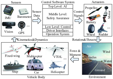
Figure 1: System structure of unmanned vehicles.

Currently, experimental testing is widely adopted because it can reflect real situations to the utmost extent. Besides, the safety problems of control systems are usually highly coupled with the actual situations. Since there is still no widely recognized safety assessment standard published for unmanned vehicle systems (both unmanned cars and aircraft), many pre-researches are proposed to comprehensively test and assess the safety of unmanned systems based on experimental methods. For example, in [6], the experimental testing and assessing method for the safety of control systems of Unmanned Aerial Vehicles (UAVs) are studied inspired by the testing methods from the airworthiness of manned aerial vehicles. However, for unmanned vehicles, the experimental testing methods are usually high-cost, inefficient, dangerous, and regulatory restricted. With the ever-increasing complexity of control systems, the experimental testing methods become increasingly inefficient in revealing potential safety issues and covering the testing cases. Besides, in experimental testing, it is usually hard to obtain the true states of unmanned vehicles (usually estimated by sensors or human perceptions) and to ensure consistency of environment variables (e.g., wind, temperature, and road condition). For example, the sensor failures may cause the vehicle state estimation inaccuracy and unreliable to reflect the true states of vehicles, so the test results in these cases are not suitable for quantitative assessment of vehicle safety. As a result, the experimental testing results usually need to be analyzed by experienced engineers to evaluate the safety level of a control system, which is not efficient, precise, and automatic enough for modern complex control systems. Due to the above disadvantages of experimental testing methods, new simulation and test methods (e.g., the real-time simulation methods [7], high-precision modeling and system identification methods [8], model-based safety assessment methods [9]) are becoming the trend for both manned and unmanned vehicles. Although experimental testing cannot be completely abandoned, simulation testing techniques are taking on more and more safety testing and assessment tasks [10].

Simulation methods for vehicle control systems can be divided into Software-In-the-Loop (SIL) simulation and Hardware-In-the-Loop (HIL) simulation. As shown in Fig. 2(b), by running the control algorithms in the same computer with the vehicle simulation model, SIL simulation can quickly test the control algorithms with the simulation speed much faster than the real world. However, the software and hardware operating environment of the SIL simulation is different from the real vehicle system, whose control algorithms are running on specific hardware (e.g., embedded systems, and industrial computers). In summary, SIL simulations can accelerate the test speed, but it is based on the expense of losing simulation credibility. To improve the simulation credibility, as shown in Fig. 2(c), HIL simulation is proposed to reflect the real operating environment of the control algorithms by using real control systems and real-time simulation computers. The HIL simulation requires the simulation model runs in real-time with the control systems, which makes it convenient to communicate with other external hardware. Currently, there are many popular simulation software supporting HIL simulations for accelerating the development efficiency, such as Airsim, SwarmSim, and other systems for UAVs [11, 12, 13], and Carsim, Apollo, and other systems for autonomous cars [14, 15, 16]. Besides, HIL simulation systems are also widely used in robotics studies to verify their algorithms [17, 18] or train the autonomous vehicle control systems [19]. These HIL simulation systems have been proven to be convenient and efficient in accelerating the development speed of control systems of unmanned vehicles, but there are still some problems. First, these HIL systems focus more on providing testing environments for the upper-level algorithms such as control algorithms, Computer Vision (CV) algorithms and Artificial Intelligence (AI) algorithms of control systems; they usually cannot simulate the low-level software (e.g., operating system, and drivers) and hardware (e.g., sensor chips and high-speed analog circuits) due to computing capability limitations. Secondly, they require to modify the code of control systems to disable the original hardware drivers and add interface programs to exchanging data with the simulation computer, which may affect the operating environment and performance of the original system (unstable and unreliable). Thirdly, the lack of widely recognized assessment methods makes it hard for people (e.g., users, manufacturers, and certification authorities) to believe the credibility of the simulation testing results for assessments and certifications.

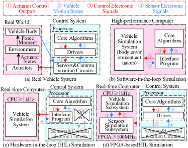
Figure 2: Comparisons between common simulation methods.

In the past, limited by the real-time response performance of simulation computers, it is hard for Central Processing Units (CPUs) [20] on simulation computers to simulate sensors or other electronic chips with high-speed interfaces or high-frequency analog circuits. For example, a nanosecond-level real-time update frequency (100MHz) is required to reliably simulate a sensor chip with the high-speed Serial Peripheral Interface (SPI), which is a difficult task for traditional CPU-based Commercial-Off-The-Shelf (COTS) simulation computers whose reliable update frequencies are usually within microsecond level. In recent years, with the utilization of Field Programmable Gate Array (FPGA) [20], COTS FPGA-based simulation computers (e.g., OPAL-RT^®/OP series and NI^®/PXI series) start to have the simulation performance of nanosecond-level real-time update frequency [7, 21]. This makes it possible to simulate almost everything (including vehicle motion, sensor chips, electric circuits, and high-speed interfaces) outside the main processor of the control systems as presented in Fig. 2(d). Besides, the tested control systems can be treated as black boxes in HIL simulation systems with no need for accessing the code or adding interface programs. Therefore, by simply replacing the sensor models, the HIL simulation system can also be applied to perform comprehensive tests for different brands of control systems.

For all simulation methods, the primary challenge is to ensure simulation credibility [22], namely making people believe the simulation results are as real as experiments in the real world. The simulation credibility (compared with real systems) mainly determined by two aspects: platform credibility and model credibility. The platform credibility can be further divided into hardware credibility and software credibility. As previously mentioned, the hardware credibility can be guaranteed by the FPGA-based HIL simulation method, while the software credibility and the model credibility are still challenges for simulation methods. The Model-Based Design (MBD) [23] method is an effective means to solve the above credibility problems by using modular visual programming technology and automatic code generation technology to standardize the modeling, developing and testing procedures of complex control systems. The MBD method can ensure the software credibility by eliminating the disturbance factors such as manual programming negligence and nonstandard development process. For example, the MathWorks^®/MATLAB (the most widely used MBD software) can ensure the generated code meet the requirements of standards and guidelines such as DO-178C. In MBD methods, the whole simulation systems can be divided into many small subsystems (modules), such as kinematic modules, GPS modules, ground modules, and propeller modules. Certification authorities can verify and validate these modules to build a standard product model database for companies to develop the vehicle prototype and the corresponding vehicle simulation system. Then, the model credibility can be guaranteed by using well-validated standard component models. What is more, with MBD method, the same component model can be applied to different types of vehicles and control systems, which may significantly improve the design, verification, validation, and certification process of the unmanned vehicle filed. For ensuring model credibility, in our previous research [24], a credibility assessment method is proposed based on experiments to assess the model credibility of HIL simulation platforms from multiple aspects, such as key performance indices, time-domain characteristics, and the frequency-domain characteristics. By combining the above methods, the credibility of the simulation platform can be guaranteed from the model, development process, and platform hardware aspects.

In this paper, a unified simulation and test platform is proposed for control systems of unmanned vehicles based on FPGA-based HIL simulation and MBD methods, aiming to significantly improve the test efficiency and safety level of control systems on unmanned vehicles. The main research contents and the corresponding contributions are listed as follows.

(i) Unified Modeling Method. There are so many in common among different types of unmanned vehicles. They should not be treated separately as more and more composite vehicles (e.g., multicopter + fixed-wing and car + fixed-wing) emerged. Therefore, a unified modeling method is proposed for all types of unmanned vehicles along with parameter measurement and identification methods to validate the obtained model and ensure simulation credibility. The corresponding content is presented in Section II.

(ii) Real-time HIL Test Platform with MBD. A real-time HIL test platform is built for the testing and assessment of control systems. The platform is capable of simulating any real-world situation outside the control software with advantages in obtaining the true states and controlling the testing variables. The utilization of MBD methods can ensure that the testing results are credible and standard-compliant. Besides, the HIL simulation method and MBD method ensure the platform can be easily applied to different brands of control systems, which is convenient for both companies and manufacturers. The corresponding content is presented in Section III.

The significant advantages of the proposed unified HIL simulation test platform are reflected in four aspects: extensibility, comprehensiveness, verification, standardization.

(i) Extensibility. By changing the parameters (e.g., weight, size, and aerodynamic coefficients) of specific subsystem modules, it is easy to extend a simulation system to other vehicle systems with similar structures. Moreover, by replacing a whole subsystem module (e.g., a propeller module to a tire module), the vehicle simulation system can be extended to other types of vehicles.

(ii) Comprehensiveness. The current simulation systems mainly focus on functional testing, i.e., whether the vehicles can work properly in normal situations. However, unmanned vehicles are safety-critical systems, and most of the effects are focused on safety testing, i.e., whether the vehicles can work safely when accident and faults happen. With the modular programming method, the fault modes, the aging process, and the probabilistic reliability property can be modeled for each subsystem module to improve the comprehensiveness of the simulation platform. Mathematically, the fault injection simulations (or other safety simulations) can be realized by online changing the module parameter or functional expressions of a subsystem module while the simulation program is running.

(iii) Verification. In practice, it is difficult to verify and validate the simulation accuracy and credibility of a complex simulation system. However, it is relatively simple to verify a small subsystem. Therefore, the modular programming method can divide a complex simulation system into many small subsystems, and verify it from lower levels to the top level. More importantly, if all subsystems used in a simulation system are well-verified modules from certification authorities, the verification efficiency can be significantly improved.

(iv) Standardization. A standard certification framework is urgently needed for unmanned vehicles to improve the testing and certification efficiency. The modular programming method is a feasible way to solve this problem with the certification framework presented in Fig. 3. In this framework, the manufactures should provide the product hardware along with a simulation model which should be fully verified and certificated by authority agencies based on the simulation data and experimental data. That coincides with the idea of Digital Twin [25] for the efficient design and testing of complex systems. Then, the vehicle companies can use the certified models for simulation system development and prototype design. Finally, the simulation results and experimental results can be applied for the certification of the unmanned vehicle.

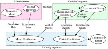
Figure 3: Certification framework for unmanned vehicles.

In Section IV, the successful application of the testing platform on multicopter vehicles with the PX4 autopilot system indicates the effectiveness of the proposed modeling and simulation methods. To verify the practicability of the proposed platform, several successful applications are presented for the multicopter rapid prototyping, estimation algorithm verification, autonomous flight testing, and automatic safety testing with automatic fault injection and result evaluation of unmanned vehicles. In the end, Section V presents the conclusions.

II Unified Modeling Method

As shown in Fig. 1, different types of vehicles (e.g., cars, aircraft, and boats) have many common features in modeling and simulation. To make the maximum utilization of these common features, a unified simulation testing system is developed with the system structure presented in Fig. 4 for all unmanned vehicle systems. In this section, the unified modeling methods for the simulation system in Fig. 4 will be introduced in detail. The hardware structure and development process for the simulation system in Fig. 4 will be introduced in Section III.

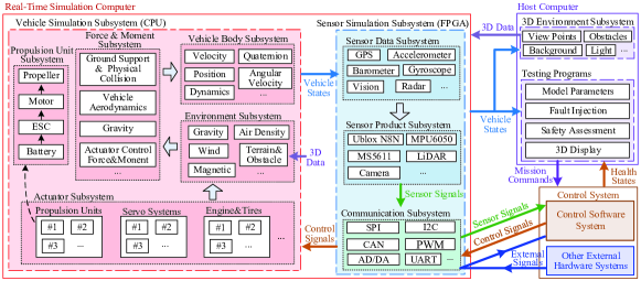
Figure 4: System structure of the simulation test platform for unmanned vehicles.

II-A Overall Vehicle Model

II-A1 Model Abstraction

In practice, a complex dynamic system usually consists of many small subsystem systems (e.g., body system and propulsion systems). Every subsystem includes input signals $\mathbf{u}_{*}$, output signals $\mathbf{y}_{*}$, parameters $\mathbf{\Phi}_{*}$, dynamic states $\mathbf{x}_{*}$, and and dynamic state and output functions $\mathbf{f}_{*}\left(\cdot\right)$ and $\mathbf{h_{*}}\left(\cdot\right)$, which can be mathematically described by the following dynamic equations

$$\left\{\begin{array}[]{c}\mathbf{\dot{x}}_{*}=\mathbf{f}_{*}\left(\mathbf{x}_{*},\mathbf{\Phi}_{*},\mathbf{u}_{*}\right)\\ \mathbf{y}_{*}=\mathbf{h_{*}}\left(\mathbf{x}_{*},\mathbf{\Phi}_{*},\mathbf{u}_{*}\right)\end{array}.\right.$$ (1)

For simplicity, a dynamic subsystem in Eq. (1) is further simplified to the following input/output form as

$$\mathbf{y}_{*}=\mathbf{S}_{*}\left(\mathbf{u}_{*}\right).$$ (2)

The system description form in Eq. 2 will be applied in the following content to describe the connection relationships among different subsystems. The subscript symbol “$*$” in Eqs. (1)(2) can be replaced by different abbreviation words to represent different dynamic systems, such as the control software system $\mathbf{S}_{\text{ctrl}}$ and the sensor simulation subsystem $\mathbf{S}_{\text{sens}}$.

II-A2 Main Framework of Simulation System

As presented in Fig. 4, the whole simulation system can be divided into three main subsystems: the vehicle simulation subsystem $\mathbf{S}_{\text{vehi}}$ (generating vehicle states according to the control signals), the 3D environment simulation subsystem $\mathbf{S}_{\text{3d}}$ (generating vision data according to the vehicle states), and the sensor simulation subsystem $\mathbf{S}_{\text{sens}}$ (generating sensor signals according to the vehicle states and vision data). Besides, there is a control system $\mathbf{S}_{\text{ctrl}}$ (generating control signals according to the sensor data) to be tested. The above connection relationships among the above four systems are mathematically described by

$$\begin{array}[]{l}\mathbf{y}_{\text{ctrl}}=\mathbf{S}_{\text{ctrl}}\left(\mathbf{u}_{\text{ctrl}}\right),\,\mathbf{u}_{\text{ctrl}}=\mathbf{y}_{\text{sens}}\\ \mathbf{y}_{\text{vehi}}=\mathbf{S}_{\text{vehi}}\left(\mathbf{u}_{\text{vehi}}\right),\,\mathbf{u}_{\text{vehi}}=\left\{\mathbf{y}_{\text{ctrl}},\mathbf{y}_{\text{3d}}\right\}\\ \mathbf{y}_{\text{3d}}=\mathbf{S}_{\text{3d}}\left(\mathbf{u}_{\text{3d}}\right),\,\mathbf{u}_{\text{3d}}=\mathbf{y}_{\text{vehi}}\\ \mathbf{y}_{\text{sens}}=\mathbf{S}_{\text{sens}}\left(\mathbf{u}_{\text{sens}}\right),\,\mathbf{u}_{\text{sens}}=\left\{\mathbf{y}_{\text{vehi}},\mathbf{y}_{\text{3d}}\right\}\end{array}$$ (3)

which is consistent with the connection relationships in Fig. 4. In the following, the unified modeling methods for the above three main subsystems will be introduced sequentially.

II-B Vehicle Simulation Subsystem

The vehicle simulation subsystem $\mathbf{S}_{\text{vehi}}$ in Fig. 4 can be further divided into four main subsystems: the actuator subsystem $\mathbf{S}_{\text{act}}$, the environment subsystem $\mathbf{S}_{\text{env}}$, the force&moment subsystem $\mathbf{S}_{\text{fm}}$, and the vehicle body subsystem $\mathbf{S}_{\text{body}}$. As shown in Fig. 5, the connection relationships of the four subsystems are mathematically described as

$$\begin{array}[]{l}\mathbf{y}_{\text{body}}=\mathbf{S}_{\text{body}}\left(\mathbf{u}_{\text{ctrl}}\right),\,\mathbf{u}_{\text{ctrl}}=\mathbf{y}_{\text{fm}}\\ \mathbf{y}_{\text{fm}}=\mathbf{S}_{\text{fm}}\left(\mathbf{u}_{\text{fm}}\right),\,\mathbf{u}_{\text{fm}}=\text{$\left\{\mathbf{y}_{\text{body}},\mathbf{y}_{\text{act}},\mathbf{y}_{\text{env}}\right\}$ }\\ \mathbf{y}_{\text{env}}=\mathbf{S}_{\text{env}}\left(\mathbf{u}_{\text{env}}\right),\,\mathbf{u}_{\text{env}}=\left\{\mathbf{y}_{\text{body}},\mathbf{y}_{\text{3d}}\right\}\\ \mathbf{y}_{\text{act}}=\mathbf{S}_{\text{act}}\left(\mathbf{u}_{\text{act}}\right),\,\mathbf{u}_{\text{act}}=\left\{\mathbf{y}_{\text{ctrl}},\mathbf{y}_{\text{body}},\mathbf{y}_{\text{env}}\right\}\end{array}$$ (4)

where $\mathbf{y}_{\text{body}}$ contains vehicle motion states (e.g., position, velocity, and attitude), $\mathbf{y}_{\text{fm}}$ denotes all the forces and moments acting on the vehicle, $\mathbf{y}_{\text{env}}$ includes environment parameters (e.g., gravity, air density, terrain, and obstacle distribution) , $\mathbf{y}_{\text{act}}$ denotes actuator states (e.g., rotating speed of rotors, and deflection angle of control surface). By combining the output signals in Eq. (4), the output set $\mathbf{y_{\text{vehi}}}$ for the vehicle simulation subsystem $\mathbf{S}_{\text{vehi}}$ is given by

$$\mathbf{y_{\text{vehi}}}\triangleq\left\{\mathbf{y}_{\text{body}},\mathbf{y}_{\text{fm}},\mathbf{y}_{\text{env}},\mathbf{y}_{\text{act}}\right\}.$$

The key modeling methods for the four subsystems in Eq. (4) will be introduced as follows.

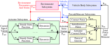
Figure 5: The structure of the vehicle simulation subsystem.

II-B1 Vehicle body subsystem

As shown in Fig. 5, the vehicle body subsystem $\mathbf{S}_{\text{body}}$ computes the vehicle states $\mathbf{y}_{\text{body}}$ according to the force and moment $\mathbf{y}_{\text{fm}}$ acting on the vehicle. In practice, based on the flat-earth assumption (ignoring the curvature of the earth in a small range) and the rigid-body assumption (the body is rigid and not flexible), most vehicle body subsystem $\mathbf{S}_{\text{body}}$ can be described by Six-Degree-of-Freedom (6-DOF) equations [26, pp. 25-54],[27, pp. 99-143]

$$\left\{\begin{array}[]{l}{}^{\text{e}}\mathbf{\dot{p}}=\mathbf{R_{\text{b}}^{\text{e}}}\cdot\mathbf{{}^{\text{b}}v}\\ \mathbf{{}^{\text{b}}\dot{v}}=-\mathbf{{}^{\text{b}}\boldsymbol{\omega}}\times\mathbf{{}^{\text{b}}v}+\left(1/m\right)\cdot\mathbf{{}^{\text{b}}F}\\ \mathbf{\dot{R}_{\text{b}}^{\text{e}}}=\mathbf{R_{\text{b}}^{\text{e}}}\cdot\left[{}^{\text{b}}\boldsymbol{\omega}\right]_{\times}\\ \mathbf{J}\cdot{}^{\text{b}}\dot{\boldsymbol{\omega}}=-^{\text{b}}\boldsymbol{\omega}\times\left(\mathbf{J}\cdot{}^{\text{b}}\boldsymbol{\omega}\right)+\mathbf{{}^{\text{b}}M}\end{array}\right.$$ (5)

where the right-superscript symbols “e” and “b” denote the North-East-Down (NED) earth frame and the Head-Right-Down body frame [26, pp. 25-54] respectively; ${}^{\text{e}}\mathbf{p}\in\mathbb{R}^{3}$ is the position vector defined in the earth frame; $\mathbf{{}^{\text{b}}v}\in\mathbb{R}^{3}$ and $\mathbf{{}^{\text{b}}\boldsymbol{\omega}}\in\mathbb{R}^{3}$ are the velocity vector and the angular velocity vector defined in the body frame; $\mathbf{{}^{\text{b}}F\in\mathbb{R}^{\mathnormal{3}}}$ and $\mathbf{\mathbf{{}^{\text{b}}M}\in\mathbb{R}^{\mathnormal{3}}}$ are the force vector and the moment vector defined in the body frame; $\mathbf{R_{\text{b}}^{\text{e}}}\in\mathbb{R}^{3\times 3}$ is the rotation matrix to transform a vector from body frame to earth frame; $\mathbf{J\in\mathbb{R}^{\text{$3\times 3$}}}$ and $m$ are the moment of inertia matrix and the mass of the vehicle. The 6-DOF dynamic equations in Eq. (5) can be applied to describe the vehicle body module $\mathbf{y}_{\text{body}}=\mathbf{S}_{\text{body}}\left(\mathbf{y}_{\text{fm}}\right)$ in Eq. (1), where the state set is $\mathbf{x}_{\text{body}}\triangleq\left\{{}^{\text{e}}\mathbf{p},\mathbf{{}^{\text{b}}v},\mathbf{R_{\text{b}}^{\text{e}}},{}^{\text{b}}\mathbf{w}\right\}$, the input set is $\mathbf{u_{\text{body}}}=\mathbf{y}_{\text{fm}}\triangleq\left\{\mathbf{{}^{\text{b}}F},\mathbf{{}^{\text{b}}M}\right\}$, the parameter set is $\mathbf{\Phi}_{\text{body}}\triangleq\left\{\mathbf{J},m\right\}$, and the output set is $\mathbf{y}_{\text{body}}\triangleq\left\{\mathbf{x}_{\text{body}},\mathbf{{}^{\text{e}}v},{}^{\text{b}}\mathbf{\dot{v}},{}^{\text{b}}\boldsymbol{\omega},\mathbf{R_{\text{b}}^{\text{e}}},\cdots\right\}$.

II-B2 Environment subsystem

As shown in Fig. 5, the environment subsystem $\mathbf{S}_{\text{env}}$ generates environment parameters $\mathbf{y}_{\text{env}}$ (e.g., air density, temperature, terrain, wind, and magnetic field) based on the position of the vehicle ${}^{\text{e}}\mathbf{p}\in\mathbf{y}_{\text{body}}$. In practice, the World Geodetic System (WGS84) model [28] is widely used to describe the shape of the earth, which can convert the position vector ${}^{\text{e}}\mathbf{p}$ to the earth Latitude-Longitude-Altitude (LLA) global position ${}^{\text{e}}\mathbf{p}_{\text{g}}\triangleq\left[\mu\,\iota\,h\right]^{\text{T}}$, where $\mu,\iota$ (unit: degree) are the latitude and longitude, and $h$ (unit: m) is the altitude. Then, the acceleration of gravity $g$ can be estimated by the WGS model [28] based on the vehicle global position ${}^{\text{e}}\mathbf{p}_{\text{g}}$. Similarly, the air density and temperature are estimated by the International Standard Atmosphere (ISA) model [29], and the magnetic field vector is estimated by the World Magnetic Model (WMM) [30]. Besides, according to the Military Specification MIL-F-8785C [31], the wind velocity disturbance vector ${}^{\text{e}}\mathbf{v}_{\text{wind}}\in\mathbb{R}^{3}$ (defined in the earth frame) can be described by the following superposition form

$${}^{\text{e}}\mathbf{v}_{\text{wind}}={}^{\text{e}}\mathbf{v}_{\text{turb}}+{}^{\text{e}}\mathbf{v}_{\text{cons}}+{}^{\text{e}}\mathbf{v}_{\text{sheer}}+{}^{\text{e}}\mathbf{v}_{\text{gust}}$$ (6)

where ${}^{\text{e}}\mathbf{v}_{\text{turb}}$ denotes the atmospheric turbulence field, ${}^{\text{e}}\mathbf{v}_{\text{\text{cons}}}$ denotes the prevailing wind field, ${}^{\text{e}}\mathbf{v}_{\text{sheer}}$ denotes the wind shear field, and ${}^{\text{e}}\mathbf{v}_{\text{gust}}$ denotes the wind gust field. There many widely used mathematical models for the wind components in Eq. (6). For example, the wind turbulence ${}^{\text{e}}\mathbf{v}_{\text{turb}}$ can be described by the Dryden Wind Turbulence Model [31].

II-B3 Actuator subsystem

As shown in Fig. 5, the actuator subsystem $\mathbf{S}_{\text{act}}$ outputs actuator state $\mathbf{y}_{\text{act}}$ according to the control input $\mathbf{y}_{\text{ctrl}}$ from the control system. In practice, it is difficult to obtain the mathematical model of an actuator system because it is usually composed by complex mechanical components along with programmable control units, such as the Electronic Speed Controller (ESC) for UAV brushless motors, and the Electronic Control Unit (ECU) for car engines and steering systems. These control units have feedback control to ensure that the actuator steady output $\delta_{\text{ss},i}$ satisfy the preprogrammed function of the input control signal $\sigma_{i}\in\mathbf{y}_{\text{ctrl}}$ under different operating environment. According to [27], a complex actuator system can be linearized to a steady-state process $f_{\text{ss},i}\left(\cdot\right)$ and a dynamic response process $G_{\text{ss},i}\left(s\right)$ around the rated operation condition. For example, a motor-propeller system with an ESC can be simplified as a first-order or second-order inertial process $G_{\text{ss},i}\left(s\right)$ and a steady-state function $f_{\text{ss},i}\left(\sigma_{i}\right)$ as

$$\delta_{i}=G_{\text{ss},i}\left(s\right)\cdot f_{\text{ss},i}\left(\sigma_{i}\right).$$ (7)

Noteworthy, $f_{\text{ss},i}\left(\cdot\right)$ can be measured by static testing, and $G_{\text{ss},i}\left(s\right)$ can be measured by system identification methods through frequency-response testing [32]. By using Eq. (7), it is easy to obtain the actuator output signal $\delta_{i}\left(t\right)$ (propeller rotating speed) under the given control signal $\sigma_{i}\left(t\right)$ (throttle control signal). Then, the control force and torque generated by the state of an actuator $\delta_{i}$ can be obtained by the ground friction model, aerodynamic model, or other mechanical models [27, 33, 34].

II-B4 Force & moment subsystem

As shown in Fig. 5, the force&moment subsystem $\mathbf{S}_{\text{fm}}$ outputs the force and moment $\mathbf{y}_{\text{fm}}\triangleq\left\{\mathbf{{}^{\text{b}}F},\mathbf{{}^{\text{b}}M}\right\}$ to the vehicle body subsystem $\mathbf{S}_{\text{body}}$. The total force $\mathbf{{}^{\text{b}}F}$ and moment $\mathbf{{}^{\text{b}}M}$ acting on a vehicle can be divided into many components from different sources. Taking the force vector $\mathbf{{}^{\text{b}}F}\in\mathbf{y}_{\text{fm}}$ (defined in the body frame) as an example, it can be described by the following superposition form

$$\mathbf{{}^{\text{b}}F}=\mathbf{{}^{\text{b}}F}_{\text{aero}}+\mathbf{{}^{\text{b}}F}_{\text{grav}}+\mathbf{{}^{\text{b}}F}_{\text{cont}}+\sum\mathbf{{}^{\text{b}}F}_{\text{act},i}$$ (8)

where $\mathbf{{}^{\text{b}}F}_{\text{aero}}\in\mathbb{R}^{\mathnormal{3}}$ denotes the aerodynamic force vector, $\mathbf{{}^{\text{b}}F}_{\text{grav}}\in\mathbb{R}^{\mathnormal{3}}$ denotes the force of gravity vector, $\mathbf{{}^{\text{b}}F}_{\text{cont}}\in\mathbb{R}^{\mathnormal{3}}$ denotes the contact force vector from ground supporting or physical collision, and $\mathbf{{}^{\text{b}}F}_{\text{act},i}\in\mathbb{R}^{\mathnormal{3}}$ denotes the control force vector generated by an actuator. Noteworthy, the above force vectors should be all transformed to the body center and projected to the body frame.

The aerodynamic force vector $\mathbf{{}^{\text{b}}F}_{\text{aero}}$ is a nonlinear function determined by the relative speed of the surrounding air ${}^{\text{e}}\mathbf{v}_{\text{rel}}$ as

$${}^{\text{e}}\mathbf{v}_{\text{rel}}\triangleq{}^{\text{e}}\mathbf{v}_{\text{wind}}-{}^{\text{e}}\mathbf{v}$$

where ${}^{\text{e}}\mathbf{v}_{\text{wind}}$ is the wind speed from the environment subsystem in Eq. (6) and ${}^{\text{e}}\mathbf{v}$ is the vehicle speed from the body subsystem in Eq. (5). The high-precision aerodynamic modeling method has been well studied in [26], which is compatible with all types of vehicles such as multicopters [27], helicopters [33] and cars [34].

The contact force $\mathbf{{}^{\text{b}}F}_{\text{cont}}$ caused by the ground supporting or physical collision can be modeled by simplifying the vehicle body shape to a cuboid or a cylinder and simplifying the contact surface to a spring-loaded system. By adjusting the spring stiffness, it is convenient to simulate physical contact on objects with different surface hardness. The terrain and obstacle information comes from the environment subsystem output $\mathbf{y}_{\text{env}}$, which further comes from the 3D environment subsystem $\mathbf{S}_{\text{3d}}$.

The actuator force vector $\mathbf{{}^{\text{b}}F}_{\text{act},i}$ can be unified described by the following nonlinear expression

$$\mathbf{{}^{\text{b}}F}_{\text{act},i}=\mathbf{f}_{\text{act},i}\left(\mathbf{\Phi}_{\text{fm}},\mathbf{y}_{\text{env}},\mathbf{y}_{\text{body}},\delta_{i}\right)$$ (9)

where $\delta_{i}\in\mathbf{y}_{\text{act}}$ is the instantaneous state of an actuator (the rotating speed of a propeller, deflection angle of a servo system, or driving torque of a tire) from the actuator module $\mathbf{S}_{\text{act}}$. Noteworthy, the expression of $\mathbf{f}_{\text{act},i}\left(\cdot\right)$ is also related to the vehicle state $\mathbf{y}_{\text{body}}$ and the environment state $\mathbf{y}_{\text{env}}$, and the methods to obtain the force model $\mathbf{f}_{\text{act},i}\left(\cdot\right)$ have been well studied in [27, 33, 34].

As shown in Fig. 6, the different types of vehicle simulation models are mainly distinguished by the actuator types and configurations. In a similar way, the actuator force models for different types of vehicles in Fig. 6 can be easily obtained with proper actuator system modeling methods.

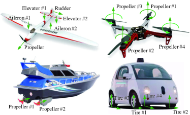
Figure 6: Actuator force models for different types of unmanned vehicles.

II-C 3D Environment Simulation Subsystem

The 3D environment subsystem $\mathbf{S}_{\text{3d}}$ in Eq. (3) aims to generate vision data $\mathbf{y}_{\text{3d}}$ based on the vehicle states $\mathbf{y}_{\text{vehi}}$ from the vehicle simulation subsystem. The vision data will be sent to the sensor subsystem to generate data for vision sensors such as camera, radars, laser range finder, etc.

Currently, many widely used 3D environment engines can be applied for vehicle vision modeling. For example, the Simulink 3D Animation Toolbox provides interfaces to conveniently access the video stream for image process and controller design in Simulink; the Airsim [11] is developed by Microsoft^® to generate high-fidelity visual and physical simulation environment using Epic Games^®/Unreal Engine 4 (UE4). Both Simulink 3D Animation Toolbox and Airsim can be applied to different types of vehicles, including aircraft and cars. There are also many 3D simulation environments exclusively developed for specific types of vehicles. For example, the Gazebo HIL simulator [16] for visual simulation of autonomous cars, and the FlightGear [35] for aircraft simulations.

These 3D simulation engines can be applied to develop the 3D environment subsystem to generate vision data (cameras), obstacle distance information (rangefinders, radars), or point cloud data (Lidar). With the development of GPU performance and 3D modeling technology, the obtained vision data $\mathbf{y}_{\text{3d}}$ will be more and more high-fidelity and realistic in the future, which will significantly improve the credibility of visual simulations.

II-D Sensor Simulation Subsystem

The sensor subsystem $\mathbf{S}_{\text{sens}}$ in Eq. (3) describes the process to transform the vehicle state $\mathbf{y}_{\text{vehi}}$ and vision data $\mathbf{y}_{\text{3d}}$ to the electric signals $\mathbf{y}_{\text{sens}}$ for the control system. Concretely, it can also be divided into three small subsystems, including the sensor data subsystem $\mathbf{S}_{\text{data}}$, the sensor product subsystem $\mathbf{S}_{\text{prod}}$ and the communication subsystem $\mathbf{y}_{\text{sens}}$. As shown in Fig. 4, their connection relationships are mathematically described as

$$\begin{array}[]{l}\mathbf{y}_{\text{data}}=\mathbf{S}_{\text{data}}\left(\mathbf{u}_{\text{data}}\right),\,\mathbf{u}_{\text{data}}=\mathbf{u}_{\text{sens}}=\left\{\mathbf{y}_{\text{vehi}},\mathbf{y}_{\text{3d}}\right\}\\ \mathbf{y}_{\text{prod}}=\mathbf{S}_{\text{prod}}\left(\mathbf{u}_{\text{prod}}\right),\,\mathbf{u}_{\text{prod}}=\mathbf{y}_{\text{data}}\\ \mathbf{y}_{\text{\text{sens}}}=\mathbf{y}_{\text{com}}=\mathbf{S}_{\text{com}}\left(\mathbf{u}_{\text{\text{com}}}\right),\,\mathbf{u}_{\text{\text{com}}}=\mathbf{y}_{\text{prod}}\end{array}$$ (10)

where $\mathbf{y}_{\text{data}}$ contains ideal data for sensors (e.g., the acceleration of accelerometers, the magnetic field of magnetometers, and the image or point cloud data of vision sensors), and $\mathbf{y}_{\text{prod}}$ is the sensor signals after adding detailed product features (e.g., noise level, temperature drift, failure mode, and camera distortion), and $\mathbf{y}_{\text{sens}}$ is the binary electrical signals transmitted to the control system for position and attitude estimation.

II-D1 Sensor Data Subsystem

As described in Eq. (10), the sensor data subsystem $\mathbf{S}_{\text{data}}$ generates the sensor data $\mathbf{y}_{\text{data}}$ (applicable for a class of sensor products) based on the vehicle state $\mathbf{y}_{\text{vehi}}$ and vision data $\mathbf{y}_{\text{3d}}$. Transformations usually required to obtained the sensor data from the vehicle states and vision data. For example, accelerometers measure the specific force (the difference between the acceleration of the aircraft and the gravitational acceleration) [36, p. 122] instead of the vehicle acceleration $\mathbf{{}^{\text{b}}\dot{v}}\in\mathbf{y}_{\text{vehi}}$. Similar computation expressions are applied to other types of sensors, such as the GPS Modules (longitude and latitude obtained from the vehicle position), electronic compasses (the magnetic field intensity obtained from the attitude and global position of the vehicle), optical flow sensors (relative velocity obtained from image stream), etc.

II-D2 Sensor Product Subsystem

The sensor product subsystem $\mathbf{S}_{\text{prod}}$ is developed to add product features (e.g., noise, vibration, and calibration) to the sensor data $\mathbf{y}_{\text{data}}$ obtained from the above sensor data subsystem $\mathbf{S}_{\text{data}}$. Given the same sensor data, different sensor products may obtain different results due to product features, so the senor product subsystem is necessary.

In most cases, given the ideal sensor data $\mathbf{x}_{\text{m}}\in\mathbf{y}_{\text{data}}$, the noise feature is mainly reflected in the noise $\mathbf{n}_{\text{a}}$ and bias drift $\mathbf{b}_{\text{a}}$ of the measured value $\mathbf{x}_{\text{m}}^{\prime}$, which can be described as [27, p. 151]

$$\begin{cases}\mathbf{x}_{\text{m}}^{\prime}&=\mathbf{x}_{\text{m}}+\mathbf{b}_{\text{a}}+\mathbf{n}_{\text{a}}\\ \mathbf{\dot{b}}{}_{\text{a}}&=\mathbf{n}_{\text{b}}\end{cases}$$ (11)

where $\mathbf{n}_{\text{a}}\sim N\left(0,\sigma_{\text{a}}^{2}\right)$ and $\mathbf{n}_{\text{b}}\sim N\left(0,\sigma_{\text{b}}^{2}\right)$ are zero-mean Gaussian noise vectors for inertial sensors. The standard deviation parameters $\sigma_{\text{a}},\sigma_{\text{b}}$ can be found in the datasheet document of a sensor product or obtained by system identification with the actual sensor output signals.

If the system is not affected by vibrations, $\sigma_{\text{a}}$ can be modeled as a constant value. When the vibration feature of a sensor is considered, the measuring noise $\mathbf{n}_{\text{a}}$ may also be affected by the vibration from may sources (e.g., engines, motors, and fuselage).Therefore, the standard deviation $\sigma_{\text{a}}$ is not always constant value, which should be modeled based on the actual system characteristics.

The calibration feature is mainly determined by the working environment of the installation configuration a sensor, which can be described as [27, p. 149]

$$\mathbf{x}_{\text{m}}^{\prime\prime}=\mathbf{T}_{\text{e}}\mathbf{K}_{\text{e}}\left(\mathbf{x}_{\text{m}}^{\prime}+\mathbf{p}_{\text{e}}\right)$$ (12)

where $\mathbf{p}_{\text{e}}$ is a constant vector for the position installation deviation, $\mathbf{T}_{\text{e}}$ is a rotation matrix for the installation deviation, $\mathbf{K}_{\text{e}}$ is a diagonal matrix for the scale deviation, and $\mathbf{x}_{\text{m}}^{\prime\prime}\in\mathbf{y}_{\text{prod}}$ is the final output data of a sensor. Eqs. (11)(12) are applicable to most types of sensors to simulate the properties of real sensor products.

There are also many methods to add product features for vision sensors. For example, the methods to add camera features (e.g., blurs, distortions, and noises) to an ideal image is introduced in [37]. Other environment factors (e.g., lighting, reflection, and fogging) can be simulated by the latest 3D engines, such as UE4.

II-D3 Communication Subsystem

The communication subsystem is developed to transform the sensor data with product features $\mathbf{y}_{\text{prod}}$ to binary electronic signals $\mathbf{y}_{\text{\text{sens}}}$ for the control system. The outputs $\mathbf{y}_{\text{prod}}$ of the above sensor product subsystem $\mathbf{S}_{\text{prod}}$ are decimal numerical signals, but binary electronic signals are required for the communication requirements between the control system and other hardware. There are many communication interfaces and protocols widely used in the vehicle control systems, such as SPI, Inter-Integrated Circuit (I²C) [38], Controller Area Network (CAN), Universal Asynchronous Receiver-Transmitter (UART), and Pulse-Width Modulation (PWM).

The mathematical model for a communication interface is usually simple, but it is hard to be simulated by a CPU-based simulation computer due to the extremely high real-time update frequency and bandwidth requirements. Taking the SPI interface as an example, the SPI interface uses four signal wires to exchange information between the master device (the main processor of the control system) and the slave device (onboard sensors). As shown in Fig. 7, the sensor has to finish the command recognition, measured data computation, and output data preparation within a small interval (after the previous byte data received and before the following byte data to be sent). In a real sensor chip, the above process is instantaneously realized by analog circuits whose time consumption can be treated as infinitely small. However, for a real-time simulation system, it usually requires a real-time update frequency at the nanosecond level to ensure that the sensor signals are correctly computed, prepared, and transmitted. For the performance requirements, this paper uses FPGA system to simulate all sensor communication features (e.g., data transmission, chip recognition, programmable setting functions), which ensures all the sensor hardware related low-level test cases can be simulated by the simulation platform.

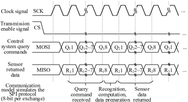
Figure 7: Communication subsystem model for SPI buses.

II-E Model Identification and Validation

The mathematical model of a subsystem can be classified into three types: the static models, the dynamic models, and the statistical models. (i) The static models are described by constant parameters that can usually be precisely measured by professional equipment. These parameters include the mass, moment of inertia, air density, aerodynamic coefficients, etc. (ii) The dynamic models are described by dynamic equations that are usually difficult to be measured by equipment directly. System identification methods [8, 32] are widely used in obtaining dynamic parameters in aircraft and vehicle systems. (iii) The statistical models are described by statistical values or stochastic processes (e.g., the sensor noise, and the atmospheric turbulence). The statistical models can be obtained by spectral analysis or statistical analysis of the output signals with enough sample data. For example, the expectation and variance of the White Gaussian noise of a sensor product in Eq. (11)(12) can be obtained by its output signals [39].

In practice, by using advanced modeling methods with enough experimental data, any vehicle system can be modeled arbitrarily close to the real system. However, a high-fidelity mathematical model usually indicates more computational complexity and cost (higher dimension and nonlinearity), so abstraction and simplification methods are important for simulation systems. The simulation credibility is the most important index in the trade-off between precision and complexity. In our previous research [24], by feeding the same signals to both the simulation system and the real system and analyzing the simulation errors, a simulation credibility assessment method is proposed to assess the simulation credibility of a simulation system from multiple aspects, such as system performance, time-domain response, and frequency-domain response. A normalized assessment index is proposed to score the simulation credibility of a subsystem under a uniform assessment criterion. The proposed method is efficient to verify and validate the simulation effect of each subsystem and the whole simulation system, which is used in this paper to ensure the credibility of the obtained vehicle subsystem models.

III Real-time HIL Test Platform with MBD

This section presents the hardware structure and development framework of the proposed HIL test platform in Fig. 4 successively.

III-A Hardware Structure of the HIL Platform

The platform hardware consists of three parts.

III-A1 Real-time Simulation Computer

A real-time simulation computer (also called real-time simulator) is a special type of computer, running Real-Time Operation System (RTOS) to ensure the simulation systems run at the same speed as the actual physical system. The latest COTS simulation computers usually provide a CPU-based system and an FPGA-based system for different requirements of real-time update frequency; the CPU-based system is better at running complex simulation models with moderate frequency requirements (usually smaller than 100KHz); the FPGA-based system is better at running simple simulation models with extremely high frequency (usually larger than 100MHz). By combining the advantages of the above two systems, the hardware structure of the proposed test platform is presented in Fig. 4, where the CPU-based system is applied to run the vehicle simulation subsystem presented in Section II-B and the FPGA-based system is applied to run the sensor simulation subsystem presented in II-D.

III-A2 Control System

The control system is the test object of the proposed test platform. The control system computes control signals for driving the actuators according to the vehicle states measured and estimated by different sensors. To ensure the control system can work normally in the proposed test platform, the original sensors should be blocked (or removed), and the sensor pins on the control system should be reconnected to the FPGA-based system of the real-time simulation computer. Then, the control system can receive the simulated sensor chip signals for full-function operation. The above process only needs to know the brands and models of sensors used in the control system, and has no requirement to access the source code or internal hardware structure. Therefore, it is practical to perform black-box testing for different control system products from different unmanned vehicle companies.

III-A3 Host Computer

A high-fidelity 3D simulation environment is also essential for training or testing the top-level algorithms, including computer vision, machine intelligence, and decision making systems. Therefore, a host computer with high-performance Graphics Processing Units (GPUs) and realistic 3D engines are used in this paper to generate vision signals to the real-time simulation computer. The latest high-end consumer GPUs (such as NVIDIA GTX2080) have been powerful enough to generate high-resolution (larger than 4K) video streaming with update frequency more than 100Hz, which is capable of simulating most vision sensors. Besides, the host computer also takes responsibility for running other auxiliary programs such as model parameter configuration program, 3D display program, ground control program, etc. Noteworthy, for different data bandwidth and real-time requirements, the connection and communication among the simulation computer and the host computer can be realized by optical fibers, network cables, serial ports, etc.

III-B Development Framework with MBD

III-B1 Modular Programming

In practice, developing a complex simulation software through hand-coding is a difficult and unreliable task due to too many mathematical operations. Any coding mistake, logical mistake, or unknown vulnerability may lead to wrong or inaccurate simulation results. The types and amounts of unmanned vehicles will be far more than manned vehicles, and the development cycles are required to be much shorter, so the traditional hand-coding methods are no longer suitable for developing simulation software for unmanned vehicles. As a result, modular (also described as graphical or visual) programming methods have been widely used in many MBD tools (e.g., MathWorks^®/Simulink and NI^®/LabVIEW). The whole simulation system presented in Section II has been divided into many simple and independent subsystems, and each subsystem can be easily realized by a visual module or block in the above MBD tools, which makes it easy to develop and test a complicated vehicle simulation system.

III-B2 Automatic Code Generation

Modular programming and automatic code generation are two of the most significant features of MBD tools such as Simulink, LabVIEW, and UE4. Simulink is better at developing complex simulation systems (such as unmanned vehicle simulation systems), and LabVIEW is better at developing hardware-closed simulation systems (such as sensors, circuits and communication signals) and deploying the simulation program to the real-time simulator. For example, the Aerospace Blockset in Simulink [40] provides many demos for quickly developing vehicle simulation systems, such as aircraft and multicopter. There are many 3D engines for developing high-fidelity vehicle 3D simulation environments. Among these engines, UE4 provides modular visual programming functions, so the UE4 environment is selected to develop 3D simulation scenes for the HIL platform.

In order to take full advantages of both MBD tools, the development process for simulation system software is shown in Fig. 8. The development process is divided into the following steps: (i) developing and verifying the vehicle simulation model in Simulink Environment; there are many powerful verifying tools in Simulink such as requirements traceability, code coverage check, document generation, etc., which guarantee the simulation software meets the standards and guidelines such as DO-178C; (ii) compiling the vehicle simulation subsystem into code, and importing it to the LabVIEW environment; (iii) building the sensor subsystem in LabVIEW and building the interfaces to communicate with other systems; (iv) generating code and executable files to deploy them to the real-time simulation computer; (v) developing the 3D simulation environment in UE4 and deploy it to the host computer. The whole development process in Fig. 8 is efficient and reliable because all coding and deploying operations are automatically finished by MBD tools without much human intervention. Therefore, it is convenient to replace some models and rebuild the simulation system for different types of vehicles or control systems.

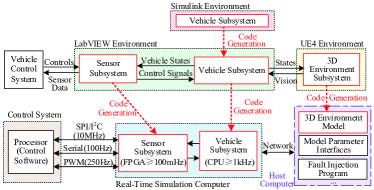
Figure 8: Code generation and deployment framework for simulation software of HIL testing platforms.

IV Verification and Application

In this section, a real-time HIL test platform is first developed for multicopter UAVs based on the proposed test platform. Then, the simulation accuracy is verified through a series of experiments. In the end, several successful applications are presented to verify the feasibility and practicability of the proposed methods in this paper.

Four videos have been published to demonstrate the development, experimental verification, and application process in this section for the proposed platform. The first video gives an overall introduction of the proposed platform along with several applications on different multicopter control systems:

https://youtu.be/nXAoLdPzz_I

The second video presents several demos of applying the proposed HIL platform to different types of vehicles (cars, copters, aircraft) with multi-vehicle traffic environment simulation:

https://youtu.be/xQUnkqH29qU

The third video presents the automatic fault injection, safety testing, and safety assessment demos:

https://youtu.be/MHieyE3hbHY

The fourth video introduces the MBD modeling and development process of the platform with experiments to quantitatively verify its simulation credibility:

https://youtu.be/ChNtkb5rrQs

We have also published the MATLAB source code and the detailed modeling tutorial to Github:

https://github.com/XunhuaDai/CopterSim

Readers can use it to rapidly develop SIL or HIL simulation systems for different types of unmanned vehicles by modifying the aerodynamic model and the actuator model.

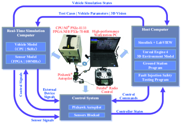
Figure 9: Hardware composition of the real-time HIL test platform

IV-A Platform Implementation

IV-A1 Hardware Composition

Based on the hardware structure presented in Fig. 4, a real-time HIL test platform is developed as shown in Fig. 9. The real-time simulation computer adopted in the platform is the NI^®/PXI simulator with CPU board: PXIe-8133 (Intel Core I7 Processor, PharLap ETS Real-Time System) and FPGA I/O Module: PXIe-7846R. The host computer is a high-performance workstation PC with professional GPU. The control system is Pixhawk autopilot, which is one of the most popular open-source autopilot hardware systems for small unmanned vehicles. All the onboard sensors (IMU, magnetometer, barometer, etc.) and external sensors (GPS, rangefinder, camera, etc.) of the Pixhawk hardware are blocked, and the sensor pins are reconnected to the FPGA I/Os to receive the simulated sensor signals through interfaces including SPI, PWM, I²C, UART, UBX, etc. In the real-time simulation computer, the update frequency of the vehicle simulation model is up to 5 kHz, and the update frequency of sensor simulation model is up to 100 MHz, whose performance is fast enough for HIL simulations of most commercial control systems. The communication among between the host computer and the real-time simulation computer is realized by network cables with TCP and UDP protocols.

IV-A2 Software Development

The simulation software of the real-time HIL test platform is developed based on the MBD method in Section III-B. The Simulink is selected to develop the vehicle simulation model because it is the most professional and widely used software for vehicle dynamic system development; the LabVIEW is selected to develop the sensor simulation model because it is efficient and convenient in real-time simulation system development; the UE4 (version: 4.22) is selected to develop the 3D environment model because it is one of the most realistic 3D engines in the development of simulation systems, games and VR systems. The Simulink, LabVIEW, and UE4 developing environments all provide convenient modular visual programming environments (see Fig. 10) and automatic code generation technology for the development of simulation systems, which are perfect for the implementation of the model-based design method. After the simulation models are all developed, the code generation and deployment framework in Fig. 8 is applied to deploy the simulation software to the real-time HIL test platform presented in Fig. 9.

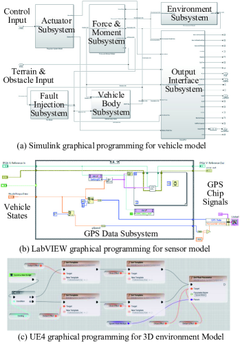
Figure 10: Modular visual programming environments in Simulink, LabVIEW, and UE4.

IV-A3 High-fidelity 3D Simulation Environment

The fidelity of the 3D simulation model is important for testing the vision-related functions of control systems, such as visual data processing, obstacle avoidance, safety decision-making, etc. With UE4, it is easy to develop high-fidelity 3D scenes for different types of vehicle in different environments. For example, as shown in Fig. 11, we have developed several 3D simulation scenes in UE4 for the HIL test platform. According to the comparisons with experiments, the display effect presented in Fig. 11 has been realistic enough for most unmanned vehicle systems to simulate the real indoor or outdoor scenes.

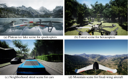
Figure 11: 3D simulation scenes developed by UE4 for different types of unmanned vehicles.

IV-B Experiments and Verification

IV-B1 Platform Feature Verification

The Pixhawk autopilot supports for running different types of flight control software systems (e.g., PX4, Ardupilot, and other embedded control software systems) in it, and also supports for controlling different types of unmanned vehicles (e.g., multicopters, small cars, and fixed-wing aircraft). Besides, the Pixhawk autopilot has a series of available hardware configurations for certain performance requirements, such as Pixhawk 1, Pixhawk 4, etc. To verify the proposed modeling method and test platform, we first apply the proposed unified modeling method in Section II to develop the simulation models for different types of unmanned vehicles, including multicopters, small cars, and fixed-wing aircraft. Then, these simulation models are deployed to the HIL test platform with the MBD framework presented in Section III. Finally, a series of tests are performed for the Pixhawk systems with various combinations of hardware configurations, software systems, and vehicle types. In our experimental tests, the four advantages of the proposed method (including extensibility, comprehensiveness, verification, and standardization) concluded in Section III-B are verified with the proposed modeling method and simulation test platform.

IV-B2 Experimental Setup

For simplicity, a quadcopter control system will be selected as the representative tested object in this section to perform quantitative verification for the proposed methods. The control system is the most widely used open-source autopilot system for small-scale unmanned vehicles, and the detailed configuration is Pixhawk 1 hardware (MCU: STM32F427, sensor: MPU6000, MS5611, LSM303D, L3GD20H, Ublox-M8N, etc.) with the PX4 control software. The quadcopter UAV is selected because it is the most representative unmanned vehicle type that covers the model characteristics (e.g., aerodynamics, ground collision, kinematics, and dynamics) and operating environments (e.g., near-ground, mid-air, indoor, outdoor, hovering flight, and forward flight) of most unmanned vehicles.

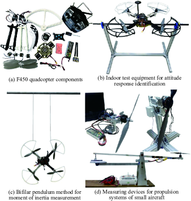
Figure 12: Verification equipment for the proposed HIL test platform.

The experimental setup is presented in Fig. 12, where an F450 quadcopter airframe (diagonal length: 450mm, weight: 1.4kg, propulsion system: DJI E310, battery: LiPo 3S 4000mAh) is selected as the experimental subject whose component diagram is shown in Fig. 12(a). In order to test the attitude dynamics and aerodynamics of the quadcopter, an indoor test bench (see Fig. 12b) is developed with the quadcopter fixed to a stiff stick (through the center of mass) with smooth bearings to minimize friction. The quadcopter is free to smoothly rotating along one axis, which makes it possible to perform sweep-frequency testing for system identification and uniform rotation testing for roll damping coefficient measurement. Figs. (c)(d) present the test benches to measure the moment of inertia and the propulsion system parameters of small-scale unmanned vehicles, and the detailed measuring methods can be found in our previous work [27, pp. 121-143]. Besides, lots of outdoor flight tests are also performed to obtain the aerodynamic coefficients of the tested quadcopter and verify the platform simulation results with actual flight results. The experimental process and results have also been presented in the video mentioned in the last subsection.

IV-B3 Simulation validation

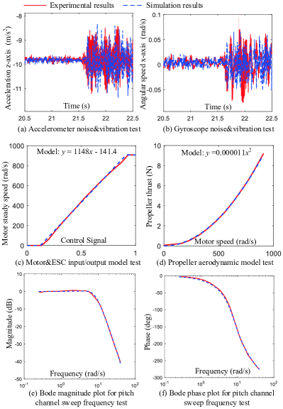
Figure 13: Comparison experiments to verify the simulation accuracy of the HIL test platform.

A series of comparative experiments are performed with the experimental test benches (see Fig. 12) and the HIL simulation test platform (see Fig. 9) to verify proposed modeling method and test platform, and several representative comparison results are presented in Fig. 13. In Figs. 13(a)(b), the accelerometer and gyroscope data obtained from the IMU sensor (MPU 6000 in Pixhawk) are presented to verify the sensor modeling methods in Section II-D. In the simulation and the experiment, the motor throttle is stepped to 50% at 21.5s to test the vibration effect caused by the high-speed rotating motors and propellers. In Figs. 13(c)(d), the propeller actuator modeling method in Section II-B is verified with the propulsion system test benches in Fig. 12(d). Besides, sweep frequency tests are performed for the quadcopter pitch channel with the test bench presented in Fig. 12(c), and the magnitude and phase curves of the Bode plots obtained by the CIFER^® software [32] are presented in Figs. 13(e)(f), respectively. From the comparative results in Fig. 13, the following conclusions can be obtained. (i) The FPGA-based HIL test platform allows using the same control system in both experiments and simulations, which minimizes the disturbing factors for result analysis and makes it convenient to acquire control system data for comparison and assessment. (ii) From the perspective of qualitative analysis, the obtained HIL test results are close to the experimental results in Fig. 13 from both time-domain and frequency-domain aspects, which verify the simulation accuracy and credibility of the proposed modeling method and test platform. (iii) The quantitative simulation credibility assessment method proposed in our previous work [24] is applied in this paper to assess and improve the simulation credibility of the HIL platform, which ensures that a high matching degree (the credibility index in [24]) larger than 90% (where 60% presents the minimum accuracy requirement, and 100% presents a perfect match) is obtained by analyzing the results between the test platform and real experimental system from the quantitative perspective.

IV-C Method Applications

This subsection presents several successful applications with the proposed test platform to increase the development, testing, and validation efficiency of multicopters.

IV-C1 Rapid Prototyping

To take maximum advantage of the proposed test platform with MBD method, a component model database is developed for the rapid development of electric multicopters. The database covers the common products on the market for multicopter propulsion systems with model parameters obtained by their product specifications and experimental data. With this model database, an online toolbox is released (URL: https://flyeval.com/) based on our previous studies [41, 42, 43] for the automatic design and performance estimation of multicopter UAVs, and a screenshot of the online toolbox is presented in Fig. 14. Users can select component products from the database to quickly assemble a multicopter to estimate its flight performance and model parameters. The toolbox has been released for more than two years, and the user feedback indicates that it can significantly improve the multicopter model development efficiency with decent simulation accuracy.

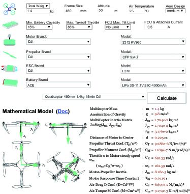
Figure 14: Screenshot of the online toolbox flyeval.com.

The level flight testing is an effective way to assess the simulation accuracy of the whole simulation model because it is the joint effect of all component models in the HIL test platform. Figs. 15(a)(b)(c) present the representative level flight testing results from a real quadcopter, an estimated model from the toolbox in Fig. 14, and a high-precision model calibrated with experimental data in Fig. 13. The quadcopter is commanded to step from hovering mode to level flight mode (the desired pitch angle is 15 degree, i.e., 0.262 rad) at 0.2s. The curve data are collected from the log data in Pixhawk after flight tests. It can be observed from Fig. 15 that the high-precision model curve almost coincides with the real experimental curve, and the estimated model curve is slightly different from the experimental curve, but the error is acceptable because it reveals most dynamic and aerodynamic characteristics of the quadcopter.

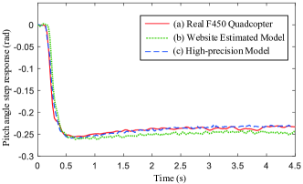
Figure 15: Level flight testing results for simulation validation.

IV-C2 Algorithm Comparison

Another important advantage of the proposed HIL test platform is that it can obtain the true states of the simulated vehicle, which is significant for comparing performance difference of control algorithms. In Fig. 16, two simulations are performed on the HIL test platform with two different estimation filter algorithms in the Pixhawk autopilot. They are the Extended Kalman filter algorithm in Fig. 16(a) and the complementary filter algorithm in Fig. 16(b), respectively. It can be observed from the result in Fig. 16 that the extended Kalman filter has a better estimation effect than complementary, which is consistent with the theoretical analysis. This conclusion is hard to obtain through experiments because a higher more precise external measuring devices (e.g., differential GPS or visual positioning systems with centimeter-level precision) is required to measure the true states of the vehicle. These external measuring devices are usually expensive and restrained. For example, the differential GPS is easy to be disturbed by flight environment factors, and its data frequency is too low (usually 5Hz), and the visual positioning system cannot be used outdoors. Therefore, the proposed test platform is a better way to acquire the true states of the vehicle for comparative analysis and performance assessment.

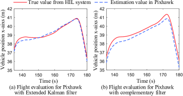
Figure 16: Comparing estimation performance of different filter algorithms in turning flight stage.

IV-C3 Normal Testing

The proposed HIL test platform makes it possible to comprehensively test the control system only with computers, which is significant in reducing cost and time relative to outdoor experiments. Fig. 17 presents an autonomous mission flight test with the proposed HIL test platform, which usually should be performed by outdoor flight tests in traditional test methods. Besides, more comparative simulation tests and experiment demonstrate that all flight tests (indoor or outdoor, manual or automatic) can be tested on the HIL test platform if the vehicle modeling is comprehensive and accurate enough.

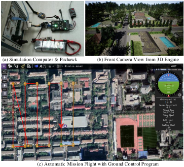
Figure 17: Autonomous mission flight testing with the proposed HIL test platform.

IV-C4 Automatic Safety Testing

With the fault modes (e.g., sensor failure, wind disturbances, and motor fault) being well modeled, the proposed HIL test platform can also be applied to perform automatic safety testing for control systems. We have developed an automatic safety testing framework (see Fig. 18) based on the HIL test platform. First, a test case database should be developed to store the vehicle command script, the fault injection triggering time, the test stop time, and the desired vehicle flight performance. In each testing case, the control system and the simulation models are automatically reinitialized to default states, and then the vehicle control system automatically controls the vehicle model in the HIL test platform to the desired state. At this moment, a fault case is injected to the HIL test platform to simulate a vehicle failure. After a period of time, the vehicle and control system states are automatically analyzed and recorded to a report. Finally, the next testing case is tested in the same way until all the testing cases are tested and evaluated. Some automatic test examples have been presented in the attached video in the previous subsection. The test results demonstrate that the platform can simulate the vehicle failure situations realistically, and the test efficiency is significantly improved with the automatic safety test method.

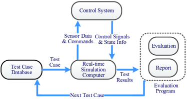
Figure 18: Automatic safety testing and validation framework.

V Conclusion and Future Work

This paper presents a unified simulation and test platform, aiming to significantly improve the development speed and safety level of unmanned vehicle control systems. A unified modular modeling framework is proposed by abstracting the common features of different types of unmanned vehicles. The application examples demonstrate this framework is efficient in developing a vehicle simulation model with compatibility for the future safety assessment and certification standards. Another key problem solved in the paper is to develop a HIL simulation test platform to ensure simulation credibility. With the model-based design method, the developing process of the simulation software can be automatized and standardized, which ensures different developers can obtain the same simulation software with credibility guaranteed by the automatic code generation tools. With the FPGA-based real-time hardware-in-the-loop simulation technology, the operating environment of the control algorithms is guaranteed by using the same control system in both experiments and simulations. After the credibility of the simulation test platform is well guaranteed, we can focus on verifying and validating the simulation models with quantitative assessment method proposed in our previous work. The proposed test platform is applied to a multicopter control system, where the accuracy and fidelity of the simulation testing results are verified by comparing with experiments. The successful applications present the advantages in the multicopter rapid prototyping, estimation algorithm verification, autonomous flight testing, and automatic safety testing with automatic fault injection and result evaluation of unmanned vehicles.

Since the test platform can provide high-fidelity and credibility simulation results, it will help to improve the training efficiency of artificial intelligence algorithms. Besides, the airworthiness for unmanned aerial vehicles require more formal, quantitative, and efficient testing methods to assess the safety level, and we will apply the proposed test platform for the safety assessment of unmanned vehicle systems.

References

- [1] H. N. Nguyen, S. Park, J. Park, and D. Lee, “A novel robotic platform for aerial manipulation using quadrotors as rotating thrust generators,” IEEE Transactions on Robotics, vol. 34, no. 2, pp. 353–369, 2018.
- [2] O. Goury and C. Duriez, “Fast, generic, and reliable control and simulation of soft robots using model order reduction,” IEEE Transactions on Robotics, vol. 34, no. 6, pp. 1565–1576, 2018.
- [3] H. Lipson and M. Kurman, Driverless: intelligent cars and the road ahead. Mit Press, 2016.
- [4] R. Mebarki, V. Lippiello, and B. Siciliano, “Nonlinear visual control of unmanned aerial vehicles in gps-denied environments,” IEEE Transactions on Robotics, vol. 31, no. 4, pp. 1004–1017, 2015.
- [5] K. Cole and A. M. Wickenheiser, “Reactive trajectory generation for multiple vehicles in unknown environments with wind disturbances,” IEEE Transactions on Robotics, vol. 34, no. 5, pp. 1333–1348, 2018.
- [6] C. M. Belcastro, D. H. Klyde, M. J. Logan, R. L. Newman, and J. V. Foster, “Experimental flight testing for assessing the safety of unmanned aircraft system safety-critical operations,” in 17th AIAA Aviation Technology, Integration, and Operations Conference. AIAA 2017-3274, 2017.
- [7] S. S. Noureen, V. Roy, and S. B. Bayne, “An overall study of a real-time simulator and application of RT-LAB using MATLAB simpowersystems,” in 2017 IEEE Green Energy and Smart Systems Conference, 2018, pp. 1–5.
- [8] M. B. Tischler, “System identification methods for aircraft flight control development and validation,” in Advances In Aircraft Flight Control, 2018, pp. 35–69.
- [9] O. Lisagor, T. Kelly, and R. Niu, “Model-based safety assessment: Review of the discipline and its challenges,” ICRMS’2011 - Safety First, Reliability Primary: Proceedings of 2011 9th International Conference on Reliability, Maintainability and Safety, pp. 625–632, 2011.
- [10] D. Jung and P. Tsiotras, “Modeling and hardware-in-the-loop simulation for a small unmanned aerial vehicle,” in AIAA Infotech@Aerospace 2007 Conference and Exhibit. AIAA 2018-2768, May. 2007.
- [11] S. Shah, D. Dey, C. Lovett, and A. Kapoor, “Airsim: High-fidelity visual and physical simulation for autonomous vehicles,” in Field and service robotics, 2018, pp. 621–635.
- [12] D. B. Worth, B. G. Woolley, and D. D. Hodson, “SwarmSim: a framework for modeling swarming unmanned aerial vehicles using hardware-in-the-loop,” The Journal of Defense Modeling and Simulation, pp. 1–20, 2017.
- [13] A. I. Hentati, L. Krichen, M. Fourati, and L. C. Fourati, “Simulation tools, environments and frameworks for UAV systems performance analysis,” 2018 14th International Wireless Communications & Mobile Computing Conference (IWCMC), pp. 1495–1500, 2018.
- [14] P. Sarhadi and S. Yousefpour, “State of the art: hardware in the loop modeling and simulation with its applications in design, development and implementation of system and control software,” International Journal of Dynamics and Control, vol. 3, no. 4, pp. 470–479, 2015.
- [15] J. R. Sylnice and G. H. Alférez, “Dynamic evolution of simulated autonomous cars in the open world through tactics,” in Proceedings of the Future Technologies Conference, 2018, pp. 257–268.
- [16] Y. Chen, S. Chen, T. Zhang, S. Zhang, and N. Zheng, “Autonomous vehicle testing and validation platform: Integrated simulation system with hardware in the loop,” in 2018 IEEE Intelligent Vehicles Symposium (IV), 2018, pp. 949–956.
- [17] A. Franchi, C. Secchi, H. I. Son, H. H. Bülthoff, and P. R. Giordano, “Bilateral teleoperation of groups of mobile robots with time-varying topology,” IEEE Transactions on Robotics, vol. 28, no. 5, pp. 1019–1033, 2012.
- [18] Y. Liu, J. M. Montenbruck, D. Zelazo, M. Odelga, S. Rajappa, H. H. Bulthoff, F. Allgower, and A. Zell, “A distributed control approach to formation balancing and maneuvering of multiple multirotor UAVs,” IEEE Transactions on Robotics, vol. 34, no. 4, pp. 870–882, 2018.
- [19] W. Li, C. W. Pan, R. Zhang, J. P. Ren, Y. X. Ma, J. Fang, F. L. Yan, Q. C. Geng, X. Y. Huang, H. J. Gong, W. W. Xu, G. P. Wang, D. Manocha, and R. G. Yang, “AADS: Augmented autonomous driving simulation using data-driven algorithms,” Science Robotics, vol. 4, no. 28, 2019.
- [20] H. Saad, T. Ould-Bachir, J. Mahseredjian, C. Dufour, S. Dennetiere, and S. Nguefeu, “Real-time simulation of MMCs using CPU and FPGA,” IEEE Transactions on Power Electronics, vol. 30, no. 1, pp. 259–267, 2015.
- [21] S. Mikkili, A. K. Panda, and J. Prattipati, “Review of real-time simulator and the steps involved for implementation of a model from MATLAB/SIMULINK to real-time,” Journal of The Institution of Engineers (India): Series B, vol. 96, no. 2, pp. 179–196, 2015.
- [22] U. B. Mehta, D. R. Eklund, V. J. Romero, J. A. Pearce, and N. S. Keim, “Simulation credibility: Advances in verification, validation, and uncertainty quantification,” NASA Ames Research Center, Moffett Field, CA United States, Tech. Rep. JANNAF/GL-2016-0001, Nov. 01, 2016.
- [23] I. MathWorks, “Model-based design - MATLAB & Simulink,” https://www.mathworks.com/solutions/model-based-design.html, Accessed May 24, 2019.
- [24] X. Dai, C. Ke, Q. Quan, and K.-Y. Cai, “Simulation credibility assessment methodology with FPGA-based hardware-in-the-loop platform,” arXiv e-prints, vol. arXiv:1907.03981, pp. 1–8, 2019. [Online]. Available: https://arxiv.org/abs/1907.03981
- [25] A. M. Miller, R. Alvarez, and N. Hartman, “Towards an extended model-based definition for the digital twin,” Computer-Aided Design and Applications, vol. 15, no. 6, pp. 880–891, 2018.
- [26] B. L. Stevens and F. L. Lewis, Aircraft Control and Simulation 2nd Edition. Wiley, New Jersey, 2004.
- [27] Q. Quan, Introduction to Multicopter Design and Control. Springer, Singapore, 2017.
- [28] R. W. Smith, Department of Defense World Geodetic System 1984: its definition and relationships with local geodetic systems. Defense Mapping Agency, 1987.
- [29] M. Cavcar, “The international standard atmosphere (ISA),” Anadolu University, Turkey, vol. 30, p. 9, 2000.
- [30] A. Chulliat, S. Macmillan, P. Alken, C. Beggan, M. Nair, B. Hamilton, A. Woods, V. Ridley, S. Maus, and A. Thomson, The US/UK world magnetic model for 2015-2020. BGS and NOAA, 2015.
- [31] D. J. Moorhouse and R. J. Woodcock, “Background information and user guide for MIL-F-8785C, military specification-flying qualities of piloted airplanes,” U.S. Air Force Wright Aeronautical Labs, Wright-Patterson AFB, OH, Tech. Rep. AFWAL-TR-81-3109, July. 1982.
- [32] R. K. Remple and M. B. Tischler, Aircraft and rotorcraft system identification: engineering methods with flight-test examples. American Institute of Aeronautics and Astronautics, 2006.
- [33] G. Cai, B. M. Chen, and T. H. Lee, Unmanned rotorcraft systems. Springer Science & Business Media, 2011.
- [34] R. Rajamani, Vehicle dynamics and control, Second Edition. Springer Science & Business Media, 2011.
- [35] A. I. Hentati, L. Krichen, M. Fourati, and L. C. Fourati, “Simulation tools, environments and frameworks for UAV systems performance analysis,” 2018 14th International Wireless Communications and Mobile Computing Conference, IWCMC 2018, pp. 1495–1500, 2018.
- [36] R. W. Beard and T. W. McLain, Small unmanned aircraft: Theory and practice. Princeton university press, 2012.
- [37] M. Kučiš and P. Zemčík, “Simulation of camera features,” Proceedings of the 16th Central European Seminar on Computer Graphics, pp. 117–123, 2012.
- [38] F. Leens, “An introduction to I2C and SPI protocols,” IEEE Instrumentation & Measurement Magazine, vol. 12, no. 1, pp. 8–13, 2009.
- [39] N. El-Sheimy, H. Hou, and X. Niu, “Analysis and modeling of inertial sensors using allan variance,” IEEE Transactions on instrumentation and measurement, vol. 57, no. 1, pp. 140–149, 2008.
- [40] S. Gage, “NASA HL-20 lifting body airframe modeled with Simulink and the aerospace blockset,” https://www.mathworks.com/help/aeroblks/nasa-hl-20-lifting-body-airframe.html, Accessed May 24, 2019.
- [41] D. Shi, X. Dai, X. Zhang, and Q. Quan, “A practical performance evaluation method for electric multicopters,” IEEE/ASME Transactions on Mechatronics, vol. 22, no. 3, pp. 1337–1348, 2017.
- [42] X. Dai, Q. Quan, J. Ren, and K.-Y. Cai, “An analytical design optimization method for electric propulsion systems of multicopter UAVs with desired hovering endurance,” IEEE/ASME Transactions on Mechatronics, vol. 24, no. 1, pp. 228–239, 2019.
- [43] X. Dai, Q. Quan, J. Ren, and C. Kai-Yuan, “Efficiency optimization and component selection for propulsion systems of electric multicopters,” IEEE Transactions on Industrial Electronics, vol. 66, no. 10, pp. 7800–7809, 2019.