Energy partition in two M-class circular-ribbon flares

Abstract

In this paper, we investigate the energy partition of two homologous M1.1 circular-ribbon flares (CRFs) in active region (AR) 12434. They were observed by SDO, GOES, and RHESSI on 2015 October 15 and 16, respectively. The peak thermal energy, nonthermal energy of flare-accelerated electrons, total radiative loss of hot plasma, and radiant energies in 1$-$8 Å and 1$-$70 Å of the flares are calculated. The two flares have similar energetics. The peak thermal energies are (1.94$\pm$0.13)$\times$10³⁰ erg. The nonthermal energies in flare-accelerated electrons are (3.9$\pm$0.7)$\times$10³⁰ erg. The radiative outputs of the flare loops in 1$-$70 Å, which are $\sim$200 times greater than the outputs in 1$-$8 Å, account for $\sim$62.5% of the peak thermal energies. The radiative losses of SXR-emitting plasma are one order of magnitude lower than the peak thermal energies. Therefore, the total heating requirements of flare loops including radiative loss are (2.1$\pm$0.1)$\times$10³⁰ erg, which could sufficiently be supplied by nonthermal electrons.

1 Introduction

Solar flares and coronal mass ejections (CMEs) are the most spectacular and energetic activities in our solar system, which have potential impact on space weather (Schwenn, 2006; Chen, 2011; Fletcher et al., 2011; Holman et al., 2011). The free magnetic energy is accumulated before flares via various mechanisms (Wiegelmann et al., 2014), such as flux emergence (Sun et al., 2012), twisting (Li et al., 2017a; Xu et al., 2017), and/or shearing motions in the photosphere (Su et al., 2007). The stored energy is impulsively released via magnetic reconnection (Priest & Forbes, 2002; Su et al., 2013; Xue et al., 2016; Li et al., 2017b) and converted to thermal energy of the directly heated plasma, kinetic energy of the bulk flow, and nonthermal energies of the accelerated electrons as well as ions (Aschwanden, 2002; Mann et al., 2006). The total energy content of flares ranges from $\sim$10²⁴ erg for the smallest ones (nanoflares) to $\sim$10³³ erg for the largest ones (X-class flares). The nonthermal electrons spiral down along the newly reconnected magnetic field lines and precipitate in the dense chromosphere, resulting in significant chromospheric evaporation and/or condensation (Brown, 1971; Fisher et al., 1985; Ning et al., 2009; Li et al., 2015; Benz, 2017; Tian & Chen, 2018). In this way, the energy in nonthermal electrons is converted through Coulomb collisions into energy in the thermal plasma.

A fraction of energetic electrons may escape into the interplanetary space along the open field and generate type III radio bursts (Mann et al., 1999; Benz, 2008). The radiations in hard X-ray (HXR), soft X-ray (SXR), ultraviolet (UV), extreme-ultraviolet (EUV), white light (WL), infrared, and radio wavelengths increase dramatically and reach an apex during the impulsive phase that spans a few to tens of minutes (Benz, 2008, see Fig. 2 for an illustration). Afterwards, the fluxes of radiation decline with time and the post-flare loops cool down via heat conduction and radiative loss (Cargill et al., 1995). Flares are classified into confined and eruptive types according to their association with CMEs (Wang & Zhang, 2007; Sun et al., 2015; Thalmann et al., 2015), although the visibility of CMEs depends greatly on flare intensity (Yashiro et al., 2005).

Although a general framework of flares has been established, the energy partition is still controversial in that the energy release, transport, and conversion processes are very complicated and strongly coupled. In fact, the situation varies from case to case. Hence, statistical studies are more appropriate to address this issue. After a detailed investigation of 24 flares observed by GOES and the Ramaty Hight Energy Solar Spectroscopic Imager (RHESSI; Lin et al., 2002), Warmuth & Mann (2016a) found that a relatively cooler plasma component (10$-$25 MK) is produced by chromospheric evaporation, while a hotter component ($\geq$25 MK) is produced by direct heating in the corona. Therefore, they concluded that electron beam heating at the chromosphere is insufficient to account for the heating of the hot thermal plasma and supplying the bolometric radiation. Conductive loss ($\propto T^{7/2}$) provides an efficient way of transporting energy from the corona to the lower atmosphere so that the energy is quickly radiated away in UV, EUV, and WL (Warmuth & Mann, 2016b).

Using coordinated observations from multiple space-borne instruments, Emslie et al. (2004) evaluated the energetics of two flare/CME events, including the energy contents of CMEs, thermal plasma of the flares, nonthermal electrons, ions, and solar energetic particles. It is concluded that, with large uncertainties, CMEs contain a dominant component of the released free energy. After refining the flare energy estimates, Emslie et al. (2005) came to a conclusion that flare and CME energies ($\sim$10³² erg) are comparable, which was further substantiated by the analysis of a different flare/CME event by Feng et al. (2013). Emslie et al. (2012) carried out a comprehensive investigation of the energetics of 38 large eruptive flares during 2002 February and 2006 December. It is revealed that the energy content in flare-accelerated electrons and ions is sufficient to supply the bolometric radiant energy.

In a big project, Aschwanden et al. (2014, 2015, 2016, 2017) studied the global energetics of flares and CMEs observed by the Atmospheric Imaging Assembly (AIA; Lemen et al., 2012) on board the Solar Dynamics Observatory (SDO) during the first 3.5 yr of its mission. The multiwavelength observations of AIA facilitate the calculation of thermal energy using the differential emission measure (DEM) distribution function. It is shown that the multithermal DEM function yields a considerably higher (multi-)thermal energy than an isothermal energy of the flares based on the same AIA data. Moreover, the nonthermal energy exceeds the thermal energy in 85% of the whole events.

In the context of standard flare model, the flare ribbons show diverse motions (Fletcher et al., 2011; Holman, 2016). In most cases, the ribbons separate as magnetic reconnection proceeds (Qiu et al., 2002; Ji et al., 2004). Apart from separation, the brightening may propagate along the ribbons (Qiu et al., 2017). For three-dimensional magnetic reconnection within the thin quasi-separatrix layers (Demoulin et al., 1996), flare ribbons propagate along the intersection of QSLs with the chromosphere (Aulanier et al., 2007). Circular-ribbon flares (CRFs) are a special kind of flares that consist of a central short ribbon and a surrounding ribbon with a circular or quasi-circular shape (e.g., Masson et al., 2009; Reid et al., 2012; Jiang et al., 2013; Joshi et al., 2015; Kumar et al., 2015; Yang et al., 2015; Hao et al., 2017; Hernandez-Perez et al., 2017; Song & Tian, 2018; Chen et al., 2019; Li & Yang, 2019; Zhang et al., 2019). Most of them are confined flares without CMEs. The magnetic topology of CRFs is usually composed of a null point, a spine, and a dome-like fan surface (Zhang et al., 2012, 2015; Masson et al., 2017; Li et al., 2018). In 2015 October, a series of homologous, short-lived CRFs occurred in active region (AR) 12434. For the first time, Zhang et al. (2016a) studied explosive chromospheric evaporation in a C4.2 CRF that occurred on October 16. Besides, Zhang et al. (2016b) reported periodic chromospheric condensation in a homologous C3.1 CRF in the same AR. So far, the energy partition in CRFs has not been explored.

In this paper, we study the energy partition in two homologous M1.1 CRFs on October 15 and 16, respectively. In Section 2, we describe the observations and data analysis. The morphological evolution of the flares and accompanying type III radio bursts are presented in Section 3. The calculations of different energy contents are elucidated in Section 4. We compare our findings with previous works in Section 5 and give a brief summary in Section 6.

2 Observations and data analysis

The M1.1 CRFs taking place in AR 12434 were observed by SDO, RHESSI, WIND, and the Nobeyama Radioheliograph (NoRH; Nakajima et al., 1994). AIA takes full-disk images in two UV (1600 and 1700 Å) and seven EUV (94, 131, 171, 193, 211, 304, and 335 Å) wavelengths. The photospheric line-of-sight (LOS) magnetograms were provided by the Helioseismic and Magnetic Imager (HMI; Scherrer et al., 2012) on board SDO. The AIA and HMI level_1 data were calibrated using the standard Solar Software (SSW) programs aia_prep.pro and hmi_prep.pro, respectively. The fluxes of the flares in 1$-$70 Å were recorded by the Extreme Ultraviolet Variability Experiment (EVE; Woods et al., 2012) on board SDO. SXR fluxes of the flares in 0.5$-$4 Å and 1$-$8 Å were recorded by GOES. The isothermal temperature ($T_{e}$) and emission measure (EM) of the SXR-emitting plasma can be derived from the ratio of GOES fluxes (White et al., 2005).

To obtain the HXR light curves, images, and spectra evolution, we use observations from RHESSI. HXR images near the flare peak times were reconstructed using the CLEAN method with an integration time of 4 s (Hurford et al., 2002). The pulse pileup correction, energy gain correction, and isotropic albedo photo correction are carried out to obtain the background-subtracted spectra. In order to derive the properties of accelerated electrons, we fit the HXR spectra by the combination of an isothermal component determined by the isothermal temperature and EM and a nonthermal component created by the thick-target bremsstrahlung of energetic electrons with a low-energy cutoff (Brown, 1971; Warmuth & Mann, 2016a). The spectra fitting is conducted using the OSPEX software built in SSW.

As a ground-based radio telescope at the Nobeyama Radio Observatory, NoRH observes the Sun at frequencies of 17 and 34 GHz with spatial resolutions of 10$\arcsec$ and 5$\arcsec$, respectively. In addition, the type III radio bursts related to the flares were recorded in the radio dynamic spectra by WIND/WAVES (Bougeret et al., 1995). WAVES consists of two detectors: RAD1 (0.02$-$1.04 MHz) and RAD2 (1.075$-$13.825 MHz). The observational parameters are summarized in Table 1.

Table 1: Description of the observational parameters

Instrument	$\lambda$	Cadence	Pixel Size
	(Å)	(s)	(″)
SDO/AIA	94$-$335	12	0.6
SDO/AIA	1600	24	0.6
SDO/HMI	6173	45	0.6
SDO/EVE	1$-$70	0.25	$\cdots$
GOES	0.5$-$4	2.05	$\cdots$
GOES	1$-$8	2.05	$\cdots$
RHESSI	3$-$50 keV	4.0	2.0
NoRH	17 GHz	1	5.0
WIND/WAVES	0.02$-$13.825 MHz	60	$\cdots$

3 Circular-ribbon flares and type III radio bursts

In Figure 1, AIA 171 Å images of the flares (CRF1 and CRF2) are displayed in the left panels (see also the online animation). Like the C-class flares reported in Zhang et al. (2016a, b), CRF1 and CRF2 feature a short inner ribbon and an elliptical outer ribbon. The length scale ($\sim$40$\arcsec$) of these compact flares is comparable to that of coronal bright points (Zhang et al., 2012). The corresponding HMI LOS magnetograms are displayed in the right panels of Figure 1. The inner and outer ribbons correspond to negative and positive polarities in the photosphere, respectively.

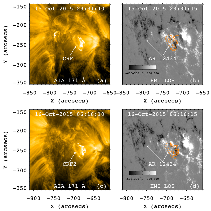
Figure 1: Top panels: AIA 171 Å image and HMI LOS magnetogram around 23:31:10 UT on 2015 October 15. CRF1 and AR 12434 are indicated by the arrows. Bottom panels: AIA 171 Å image and HMI LOS magnetogram around 06:16:10 UT on 2015 October 16. CRF2 and AR 12434 are indicated by the arrows. Intensity contours of the EUV images are superposed on the magnetograms with orange lines. (An animation of this figure is available.)

Figure 2 shows twelve snapshots of the AIA 304 Å images (see also the online animation). The two flares have some kind of similarity in morphological evolution. The inner ribbon and northwest part of outer ribbon brightened first, which was followed by brightening of the southeast part of outer ribbon (see panels (b) and (h)). Afterwards, the brightness of flare ribbons declined with time. Since the ribbon separation in confined flares is more or less static (Hinterreiter et al., 2018), the areas of CRFs did not change remarkably as expected.

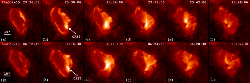
Figure 2: Snapshots of the AIA 304 Å images with a field of view of 60$\arcsec$$\times$60$\arcsec$ during CRF1 (top panels) and CRF2 (bottom panels). (An animation of this figure is available.)

In Figure 3, the SXR light curves of CRF1 are plotted in panel (a). The SXR flux in 1$-$8 Å increases rapidly from $\sim$23:27 UT until the peak value at $\sim$23:31 UT, before a gradual decline until $\sim$23:50 UT. Therefore, the lifetime of CRF1 is $\sim$23 minutes. The dashed line signifies the background flux, which will be subtracted to get a net SXR irradiance (see Figure 7(a)). Figure 3(b) shows the time evolutions of the isothermal temperature ($T_{e}$) and EM of the SXR-emitting plasma, which will be used to calculate the total radiated energy from the SXR-emitting plasma. The temperature reaches a peak value of 14.7 MK at 23:30:15 UT. The EM reaches a peak value of 0.7$\times$10⁴⁹ cm^-3 at 23:32:26 UT. The light curve in 1$-$70 Å is displayed in Figure 3(c), with a peak value at 23:32:54 UT. The dashed line represents the background flux, which will be subtracted to get a net irradiance (see Figure 7(c)). The corrected count rates at different energy bands are plotted with different colors in Figure 3(d). The peak time of nonthermal flux at 25$-$50 keV at $\sim$23:28:20 UT is indicated by the red dashed line.

In Figure 5, the full-disk radio image in 17 GHz at 23:28:30 UT is demonstrated in panel (a). A closeup of CRF1 is shown in panel (b). Due to the lower resolution of NoRH compared with AIA, the flare is a single, bright source. Time evolution of the integral flux of CRF1 is plotted in Figure 3(e). The peak time of radio flux coincides with that of HXR flux at 25$-$50 keV, confirming the nonthermal nature of emissions from the flare-accelerated, high-energy electrons. Figure 3(f) shows the time evolution of normalized integral intensity of CRF1 in 1600 Å.

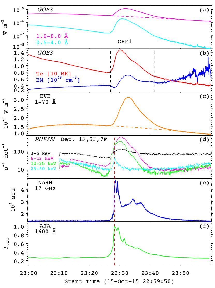
Figure 3: (a) SXR light curves of CRF1 in 0.5$-$4 Å and 1$-$8 Å. The magenta dashed line represents the background intensity. (b) Time evolutions of temperature ($T_{e}$) and emission measure (EM) derived from GOES observations. The black dashed lines represent the lower and upper limits of integrals. (c) Light curve of CRF1 in 1$-$70 Å. The orange dashed line represents the background intensity. (d) HXR light curves of CRF1 at different energy bands. (e) Radio light curve of CRF1 in 17 GHz. (f) UV light curve of CRF1 in 1600 Å. The red dashed line in panels (d)-(f) denote the peak time at 23:28:20 UT.

Like in Figure 3, the light curves of CRF2 in various wavelengths are drawn in Figure 4. The SXR flux in 1$-$8 Å starts to increase at $\sim$06:11 UT and reaches the apex at $\sim$06:16 UT, followed by a gradual decline until $\sim$06:35 UT. Therefore, the lifetime of CRF2 is $\sim$24 minutes. The maximal isothermal temperature (16.8 MK) of CRF2 is slightly higher than that of CRF1, while the maximal EM of CRF2 is slightly lower than that of CRF1. In Figure 5, the full-disk radio image in 17 GHz at 06:13:48 UT on October 16 is displayed in panel (c), and a closeup of CRF2 is displayed in panel (d). Time evolution of the integral radio flux of CRF2 is plotted in Figure 4(e). Likewise, the time evolution of normalized integral intensity of CRF2 in 1600 Å is shown in Figure 4(f). The simultaneous peak time at 06:13:48 UT is indicated by the red dashed line.

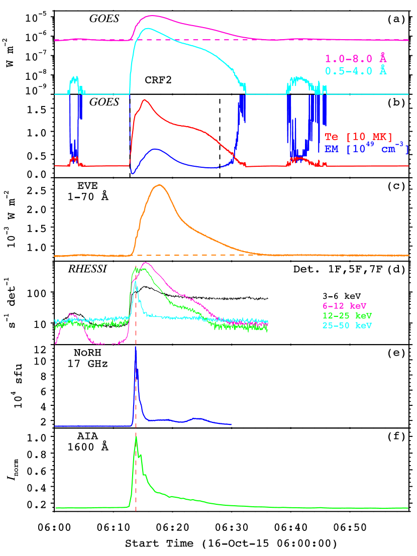
Figure 4: Same as Figure 3, but for CRF2. The red dashed line in panels (d)-(f) denote the peak time at 06:13:48 UT.

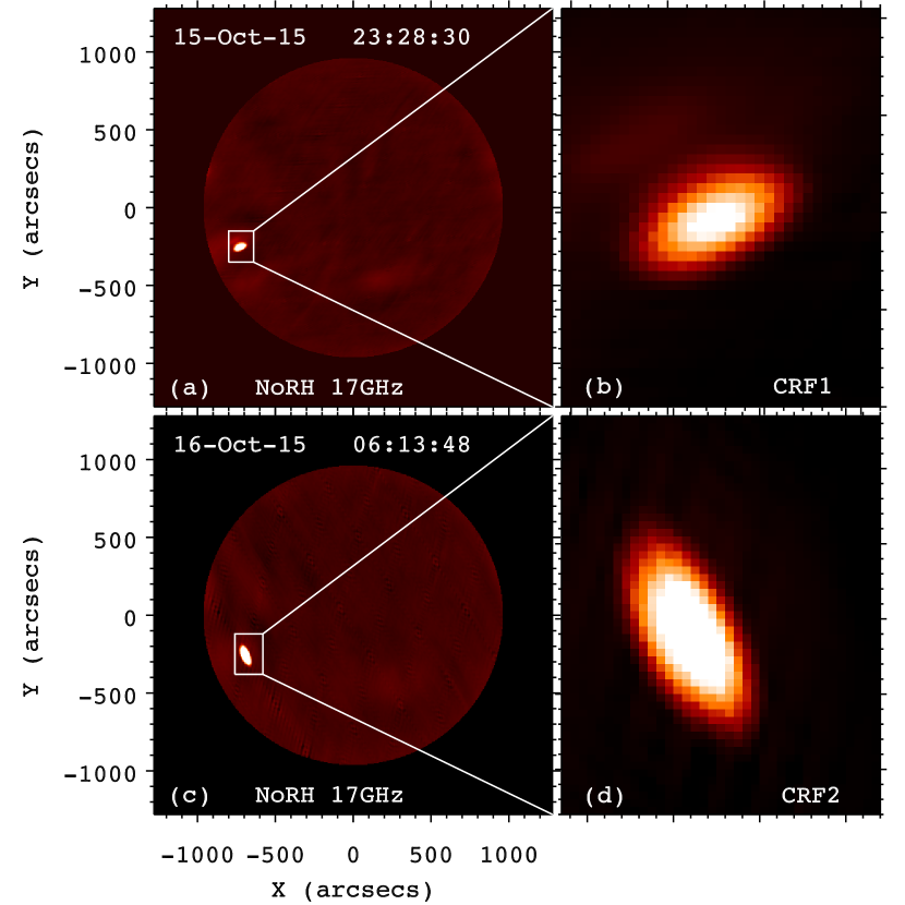
Figure 5: Left panels: Full-disk radio images in 17 GHz on October 15 and 16. Right panels: Closeups of CRF1 and CRF2.

Like the C3.1 CRF reported by Zhang et al. (2016b), both CRF1 and CRF2 were associated with type III radio bursts, which are pointed by the arrows in the radio dynamic spectra recorded by WIND/WAVES (see Figure 6). The starting times of radio bursts were consistent with the peak times in 17 GHz, implying a common origin of the radio emissions. The flare-accelerated nonthermal electrons streaming down into the chromosphere create strong emission in 17 GHz via gyro-synchrotron radiation mechanism, while those escaping from the corona along open field lines create type III bursts via plasma radiation mechanism.

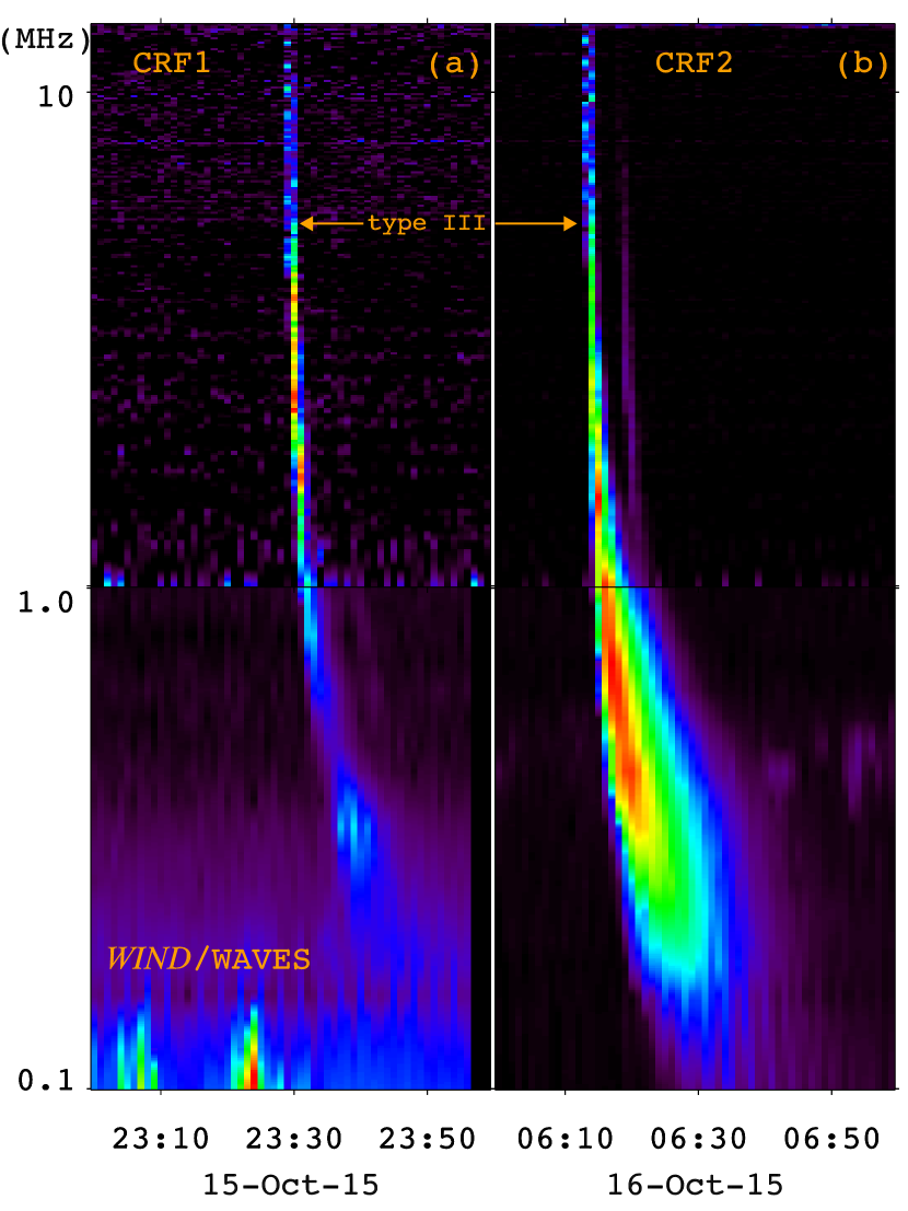
Figure 6: Radio dynamic spectra recorded by WIND/WAVES during CRF1 and CRF2. The arrows point to the type III radio bursts associated with the flares.

4 Energy partition

4.1 Radiated energy in GOES 1$-$8 Å

In this Section, we focus on the different energy contents of the confined flares. First of all, we calculate the radiated energy in GOES 1$-$8 Å. As mentioned in Emslie et al. (2012) and Feng et al. (2013), the contribution of background radiation should be removed. In the original 1$-$8 Å light curves, a few data points before $t_{sta}$ and after $t_{end}$ in Table 2 are extracted and used for a quadratic fitting. The background light curves are obtained based on the results of fitting. The background-subtracted light curves in 1$-$8 Å ($f_{1-8}$) are plotted in the top panels of Figure 7. The radiated energy is calculated by integrating the background-subtracted light curve,

$$U_{1-8}=2\pi d^{2}\int_{t_{1}}^{t_{2}}f_{1-8}(t)dt,$$ (1)

where $d\approx 1.496\times 10^{8}$ km (1 AU) represents the distance between the Sun and the Earth. The lower limit ($t_{1}$) of integral is defined to be the start time of a flare, which is listed in the fourth column of Table 2. The upper limit ($t_{2}$) of integral is defined to be the time when $f_{1-8}$ drops to 10% of the maximal value. The time of $t_{2}$ is 23:41:20 UT for CRF1 and 06:28:00 UT for CRF2 (see also top panels of Figure 7). The calculated radiated energies, being 5.50$\times$10²⁷ erg for CRF1 and 6.24$\times$10²⁷ erg for CRF2, are listed in the seventh column of Table 2. A bar chart of the energy contents is shown in Figure 12.

The definition of $t_{2}$ may influence the value of $U_{1-8}$. For example, if $t_{2}$ is taken to be the time when $f_{1-8}$ drops to 5% of the maximal value, then $U_{1-8}$ increases by a factor of 1.8% for CRF1 and 2% for CRF2, respectively.

4.2 Radiated energy in EVE 1$-$70 Å

Like in 1$-$8 Å, we extract a few data points from the original 1$-$70 Å light curves before performing a quadratic fitting and calculating the background light curves. The background-subtracted light curves in 1$-$70 Å ($f_{1-70}$) are plotted in the middle panels of Figure 7. The radiated energies are calculated by integrating the background-subtracted light curves,

$$U_{1-70}=2\pi d^{2}\int_{t_{1}}^{t_{2}}f_{1-70}(t)dt.$$ (2)

The lower and upper limits of integral have similar definitions as those in 1$-$8 Å. The times of $t_{1}$ are listed in the fourth column of Table 2. The time of $t_{2}$ is 23:43:00 UT for CRF1 and 06:30:10 UT for CRF2 (see also middle panels of Figure 7). The calculated radiated energies, being 1.12$\times$10³⁰ erg for CRF1 and 1.28$\times$10³⁰ erg for CRF2, are listed in the eighth column of Table 2. It is noted that the total radiated energies in 1$-$70 Å are $\sim$200 times larger than those in 1$-$8 Å.

Similarly, the definition of $t_{2}$ may influence the value of $U_{1-70}$. If $t_{2}$ is taken to be the time when $f_{1-70}$ drops to 5% of the maximal value, then $U_{1-70}$ increases by a factor of 1.8% for CRF1 and 2.3% for CRF2, respectively.

Unfortunately, there were no observations of flux in 70$-$370 Å from SDO/EVE during the flares, so that precise calculation of the radiated energy in 70$-$370 Å is unavailable. However, assuming that the ratio ($\sim$30) of radiation in 1$-$70 Å to that in 70$-$370 Å for X-class flares (Feng et al., 2013) is applicable to CRFs, the radiated energies in 70$-$370 Å of CRF1 and CRF2 are roughly estimated to be 3.73$\times$10²⁸ erg and 4.26$\times$10²⁸ erg, respectively. The total radiated energies in 1$-$370 Å of CRF1 and CRF2 amount to 1.16$\times$10³⁰ erg and 1.32$\times$10³⁰ erg accordingly. Woods et al. (2004) investigated the contribution of solar UV variation to the total solar irradiance (TSI) of the X17 flare on 2003 October 28. It is found that the combined contribution of radiation from XUV (0$-$270 Å) and EUV (270$-$1200 Å) to TSI is $\sim$20%. That is to say, TSI is a factor of $\sim$5 larger than the radiation in 0$-$1200 Å, in which the radiation in 1$-$370 Å plays a predominant role. Based on this assumption, we can deduce the TSI for CRF1 and CRF2, being 5.8$\times$10³⁰ erg and 6.6$\times$10³⁰ erg (see Figure 12).

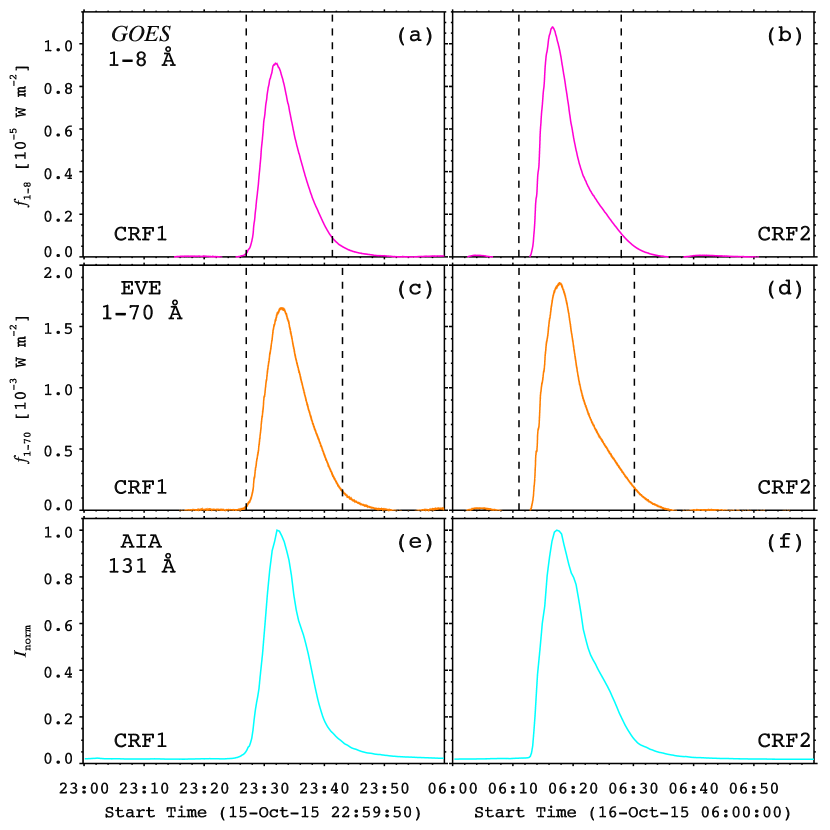
Figure 7: (a)-(d) Background-subtracted light curves in 1$-$8 Å and 1$-$70 Å of the two flares. The dashed lines denote the lower and upper time limits of integrals. (e)-(f) Light curves of the flares in 131 Å.

4.3 Radiated energy from the SXR-emitting plasma

The total optically thin radiative loss from the SXR-emitting plasma can be obtained based on the observed EM and $\Lambda(T_{e})$,

$$T_{rad}=\int_{t_{1}}^{t_{2}}\mathrm{EM}(t)\times\Lambda(T_{e}(t))dt,$$ (3)

where $\Lambda(T_{e})$ denotes the radiative loss rate (Cox & Tucker, 1969). EM and $T_{e}$ are derived from GOES observations (see Figure 3(b) and Figure 4(b)). The lower limit ($t_{1}$) and upper limit ($t_{2}$) of the integral are the same as those in Equation 1. For CRF2, the profiles of $T_{e}$ and EM are abnormal before 06:12:48 UT. Therefore, the time of $t_{1}$ for CRF2 is taken to be 06:12:48 UT. In Figure 8, the profile of $\Lambda(T_{e})$ obtained from CHIANTI 8.0 database assuming coronal abundances is adopted for calculation (Del Zanna et al., 2015). The total radiative loss from the hot plasma of CRF1 and CRF2, being 2.26$\times$10²⁹ erg and 1.41$\times$10²⁹ erg, are listed in the ninth column of Table 2. The radiative losses of the flares are $\sim$40 and $\sim$20 times larger than the radiations in 1$-$8 Å for CRF1 and CRF2, which is consistent with previous results that radiative output in 1$-$8 Å is one order of magnitude lower than the radiative loss (Feng et al., 2013). The values of $T_{rad}$ increase by a factor of $\sim$12% when $t_{2}$ changes like in Section 4.1.

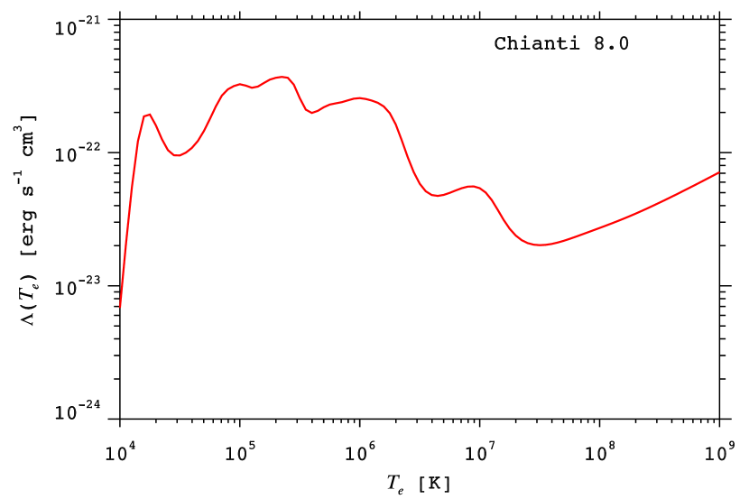
Figure 8: Radiative loss rate $\Lambda(T_{e})$ as a function of temperature ($T_{e}$) obtained from CHIANTI 8.0 database.

4.4 Peak thermal energy of the SXR-emitting plasma

The thermal energy of the SXR-emitting plasma can be expressed as

$$E_{th}=3n_{e}k_{B}T_{e}fV=3k_{B}T_{e}\sqrt{\mathrm{EM}\times fV},$$ (4)

where $n_{e}=\sqrt{\mathrm{EM}/V}$ is the electron number density, $k_{B}=1.38\times 10^{-16}$ erg K^-1 is the Boltzmann constant, $f\approx 1.0$ is the volumetric filling factor, and $V$ is the volume of the SXR-emitting plasma (Emslie et al., 2012; Feng et al., 2013). Assuming that $V$ is an invariable, then $E_{th}$ reaches the peak value when $T_{e}\sqrt{\mathrm{EM}}$ is maximal (see Figure 3(b) and Figure 4(b)).

To get a better estimation of $V$, we use two independent methods. As pointed out by O’Dwyer et al. (2010), the dominant contribution of flare spectrum for AIA 131 Å channel comes from the Fe xxi line with formation temperature of $\log T\approx 7.05$. In the bottom panels of Figure 7, light curves of the flares in 131 Å are plotted with cyan lines. It is evident that the 131 Å irradiance is well correlated with $f_{1-8}$. Therefore, the hot plasma observed in 131 Å during a flare is a good proxy of the SXR-emitting plasma (Fletcher et al., 2013). In Figure 9, the left panels demonstrate the 131 Å images 10 minutes after the peak times ($t_{peak}$ in Table 2), since the images at the peak times are severely saturated. The total areas ($A_{131}$) of the flares can be obtained by setting a threshold of intensity, which is $\sim$5 times larger than the average intensity of a nearby quiet region. Considering that the flares were close to the limb, the projection effect is corrected by multiplying a factor of $(\cos\mu)^{-1}$, where $\mu$ denotes the longitude of flare core. The corresponding volume $V_{131}$ is defined as $A_{131}^{3/2}$. The values of $A_{131}$ and $V_{131}$ are listed in the second and third columns of Table 3. If the threshold intensity is set to be $\sim$6 times larger than the quiet region intensity, the areas in 131 Å drop by a factor of 6%$-$8% and the volumes decrease by a factor of 10%$-$12%, accordingly.

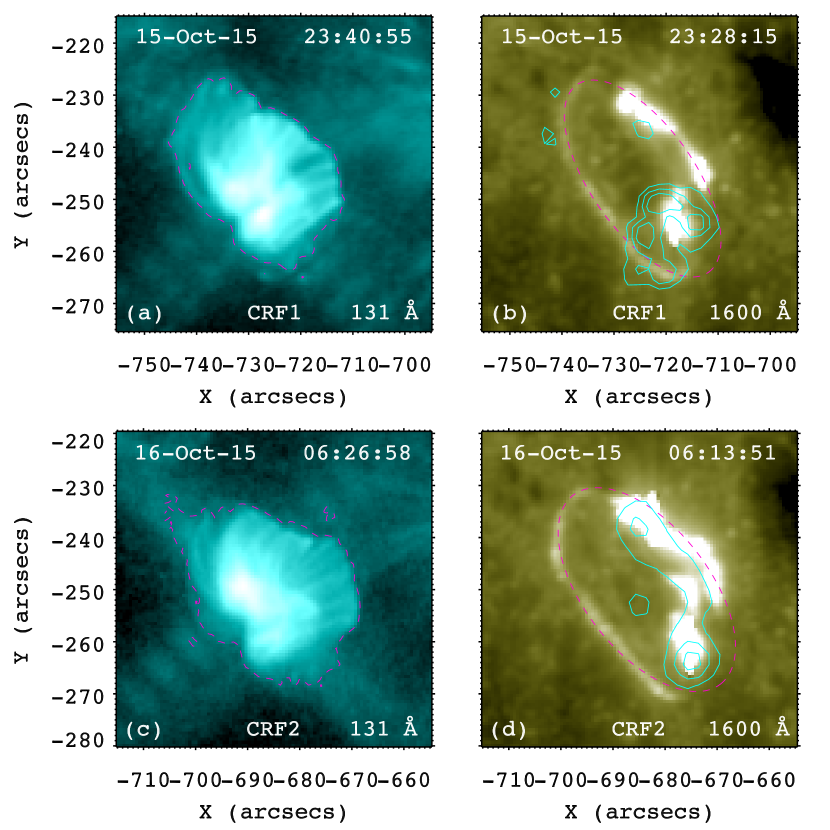
Figure 9: Left panels: AIA 131 Å images of the flares $\sim$10 minutes after the peak times. Intensity contours of the images are overlaid with magenta dashed lines. The flare area in 131 Å is calculated by summing up the pixels inside the contours. Right panels: AIA 1600 Å images of the flares at their peak times. Intensity contours of the HXR images at 12$-$25 keV are overlaid with cyan solid lines. Ellipse fittings of the outer ribbons are overlaid with magenta dashed lines. The flare area in 1600 Å is represented by the area of ellipses. (An animation of this figure is available.)

The second approach to calculating the flare area is based on the fact that the outer ribbons of CRFs mapping the footprints of the post-flare loops in the chromosphere hardly expand with time. In Figure 9, the right panels demonstrate the 1600 Å images at their peak times when the ribbons are the most noticeable (see Figure 3(f) and Figure 4(f)). Since the outer ribbons are not fully closed, we perform an ellipse fitting of the outer ribbons (magenta dashed lines). Hence, the flare areas in 1600 Å ($A_{1600}$) are represented by the areas of ellipses after correcting the projection effect. The corresponding volume $V_{1600}$ is defined as $A_{1600}^{3/2}$. The values of $A_{1600}$ and $V_{1600}$ are listed in the fourth and fifth columns of Table 3. It is obvious that both area and volume in 131 Å and 1600 Å are close to each other, suggesting that the two methods are reasonable. By adopting the mean values of $\bar{V}$ in the last column of Table 3 and peak EM during the flares, the mean electron number density ($\bar{n}_{e}$) of the hot plasma is estimated to be $\sim$2.2$\times$10¹⁰ cm^-3 for CRF1 and $\sim$1.9$\times$10¹⁰ cm^-3 for CRF2. The peak thermal energies of CRF1 and CRF2 are calculated to be 1.81$\times$10³⁰ erg and 2.06$\times$10³⁰ erg. They are listed in the tenth column of Table 2 (see also Figure 12). The increases of threshold intensity in 131 Å have marginal influence (5.5%$-$6.5%) on the final estimation of peak thermal energies. Combing the peak thermal energy and radiative loss, the total energy required to heat and maintain the hot plasma at temperatures near 10 MK are $\geq$2.0$\times$10³⁰ erg for CRF1 and $\geq$2.2$\times$10³⁰ erg for CRF2, respectively.

4.5 Energy in flare-accelerated electrons

In Figure 10, three characteristic RHESSI spectra made from detector 5 near the peak time of 25$-$50 keV flux of CRF1 are displayed. The integration time is 20 s (Feng et al., 2013).

The distribution of injected nonthermal electrons $F_{0}(E_{0})$ is assumed to be in the form of single power law (Saint-Hilaire & Benz, 2005):

$$F_{0}(E_{0})=A_{0}E_{0}^{-\delta},E_{0}\geq E_{c},$$ (5)

where $A_{0}$ is a normalized parameter of the total electron flux (in unit of 10³⁵ electrons s^-1), $E_{c}$ signifies the low-energy cutoff, and $\delta$ denotes the power-law index. In each panel, the fitted thermal component is drawn with a red line, while the nonthermal component is drawn with a blue line. Likewise, three characteristic spectra and results of fitting for CRF2 around 06:14 UT are displayed in Figure 11. As expected, the isothermal temperature from RHESSI observation is systematically higher than that from GOES observation, which is explained by the fact that RHESSI is more sensitive to high-temperature plasma (Warmuth & Mann, 2016a, b). The temperature exceeds 25 MK only at one moment (see Figure 11(a)), implying the existence of direct-heated super-hot plasma (Caspi et al., 2014; Warmuth & Mann, 2016a, b). For each flare, EM increases with time, which is consistent with the occurrence of chromospheric evaporation that quickly responds to the injection of electrons (Fisher et al., 1985; Graham & Cauzzi, 2015). The values of $\delta$ in the range 4$-$9 are close to those of M1.0 flare on 2010 August 7 (Fletcher et al., 2013).

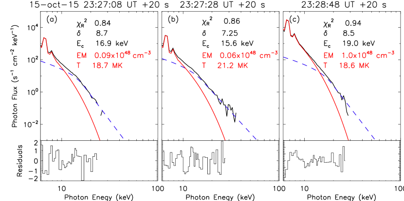
Figure 10: Three characteristic HXR spectra (black solid lines) and the fitted thermal (red solid lines) and nonthermal (blue dashed lines) components during CRF1. The isothermal temperature and EM of the thermal component are labeled. The low-energy cutoff ($E_{c}$), spectral index ($\delta$) of nonthermal electrons, and $\chi_{R}^{2}$ of the residuals are also labeled.

By comparing the spectra in Figure 10 and Figure 11, it is revealed that the electrons are accelerated to higher energies by CRF2 than CRF1. Meanwhile, the spectra indices of CRF2 are a factor of $\sim$1.5 harder than those of CRF1, indicating that CRF2 is more energetic than CRF1. The low-energy cutoffs (15$-$20 keV) of the two flares, however, do not have considerable difference.

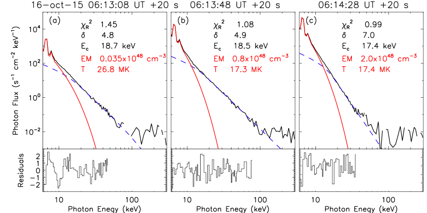
Figure 11: Same as Figure 10, but for CRF2.

The accumulated energy carried by nonthermal electrons above $E_{c}$ is derived by integrating the injected power with time,

$$E_{nt,e}=A_{nt}\int_{t_{1}^{\prime}}^{t_{2}^{\prime}}\int_{E_{c}}^{E_{H}}E_{0}F_{0}(E_{0}){dE_{0}dt},$$ (6)

where $A_{nt}$ is the electron injection area, $E_{H}$ is fixed at 30 MeV (Emslie et al., 2012; Warmuth & Mann, 2016a), $t_{1}^{\prime}$ and $t_{2}^{\prime}$ stand for the lower and upper time limits of integral. For CRF1, $t_{1}^{\prime}$ and $t_{2}^{\prime}$ are set to be 23:27 UT and 23:47 UT. For CRF2, they are set to be 06:11 UT and 06:31 UT, respectively. It is noticeable that the predominant input of nonthermal energy happens around the peak time of HXR above 25 keV. The contribution of nonthermal energy well after the peak time is negligible. The nonthermal energies in electrons are calculated by summing over all time intervals between $t_{1}^{\prime}$ and $t_{2}^{\prime}$, which are listed in the last column of Table 2. It is obvious that the nonthermal energy input by flare-accelerated electrons is sufficient to explain the heating requirement of hot plasma including the radiative loss.

Compared with the energy in electrons, a quantitative calculation of the nonthermal energy in flare-accelerated ions is much more difficult. In this work, we might as well estimate the energy in ions according to previous statistical works. The mean ratio of energy in ions to that in electrons is reported to be $\sim$1/3 (Emslie et al., 2012; Aschwanden et al., 2017). Hence, the nonthermal energy in ions for CRF1 and CRF2 are 1.1$\times$10³⁰ erg and 1.5$\times$10³⁰ erg, respectively. The total nonthermal energy including electrons and ions for CRF1 and CRF2 are thus 4.3$\times$10³⁰ erg and 6.1$\times$10³⁰ erg (see Figure 12). Our results are in accordance with previous conclusion that the thermal and nonthermal energies are of the same magnitude (Holman et al., 2003; Saint-Hilaire & Benz, 2005).

So far, it is still controversial whether the energy content in flare-accelerated electrons and ions is sufficient to account for the bolometric radiation (i.e., TSI). On one hand, Emslie et al. (2012) concluded with caution that there is sufficient energy in the flare-accelerated particles to account for the total bolometric radiation, though the mean ratio of energy in accelerated particles to the bolometric radiated energy is $\sim$0.7 in their sample. On the other hand, Warmuth & Mann (2016b) insisted that the nonthermal energy input by energetic electrons is insufficient to account for the total heating requirement of the hot plasma or for the bolometric loss, especially for weak flares. In this study, the estimated nonthermal energies of CRFs are very close to the estimated bolometric radiation (see Section 4.2 and Figure 12). Hence, our result is in favor of the conclusion by Emslie et al. (2012), albeit in-depth investigation is needed in the future.

In a comprehensive investigation of the global energetics of $\sim$400 flare/CME events observed by SDO, Aschwanden et al. (2017) concluded that nonthermal energy of flare-accelerated particles, the energy of direct heating, and the energy in CMEs, which are the primary processes in an eruptive flare, account for $\sim$87% of the dissipated magnetic energy. The nonthermal energies in electrons and ions account for more than 2/3 of the dissipated energy. Therefore, the dissipated magnetic energies of CRF1 and CRF2 can be estimated, being $\sim$6.4$\times$10³⁰ erg and $\sim$9.1$\times$10³⁰ erg (see Figure 12). It should be emphasized that the estimated dissipated free energy is an upper limit, since the CRFs in our work are confined events without CMEs and a larger part of dissipated energy are involved in particle acceleration. The reason why we do not perform a nonlinear force-free field extrapolation is that AR 12434 was close to the limb, so that the measurement of photospheric vector magnetograms was less reliable.

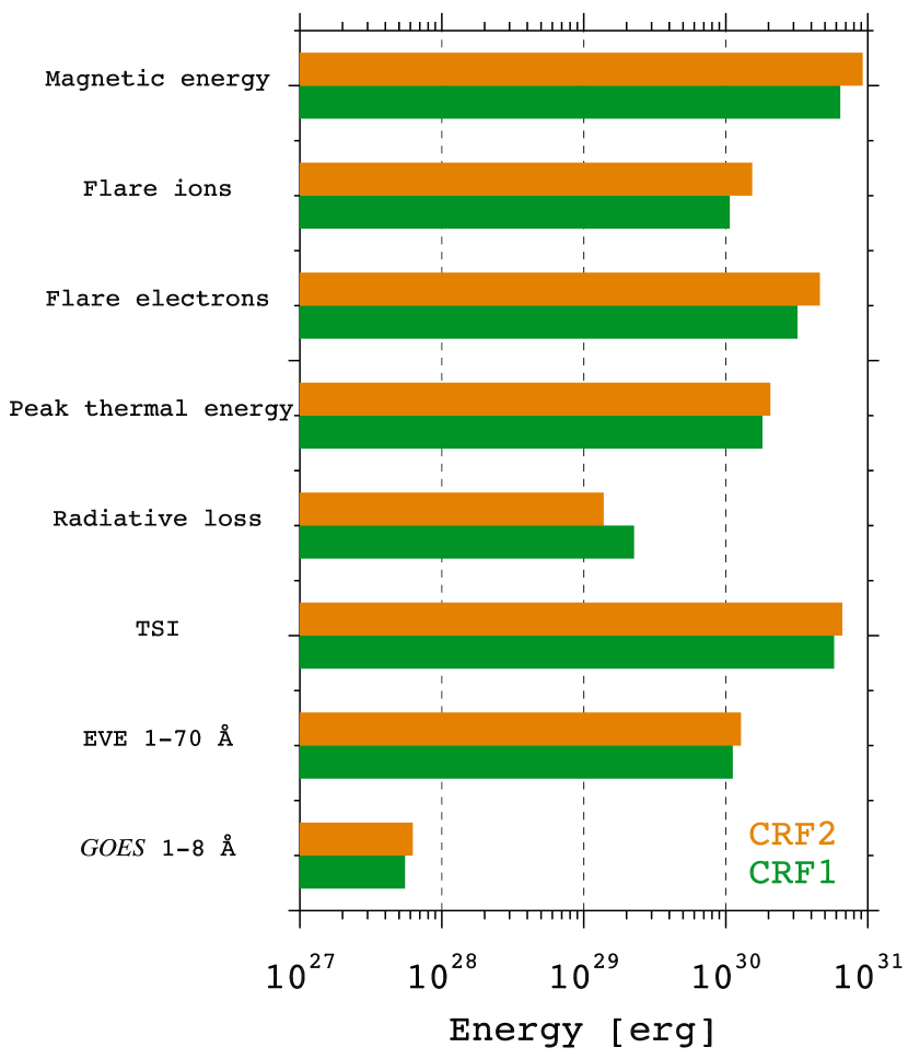
Figure 12: Bar chart showing the different energy components of CRF1 (green bars) and CRF2 (orange bars). The TSI, nonthermal energy of flare-accelerated ions, and dissipated magnetic energy are estimated from previous statistical results.

Table 2: Event list with component energies ($\times$10³⁰ erg) and the ratios (CRF2/CRF1)

flare	Class	Date	$t_{sta}$	$t_{peak}$	$t_{end}$	1$-$8 Å	1$-$70 Å	$T_{rad}$	$E_{th}$	$E_{nt,e}$
CRF1	M1.1	15-Oct-15	23:27	23:31	23:50	5.50e-3	1.12	2.26e-1	1.81	3.2
CRF2	M1.1	16-Oct-15	06:11	06:16	06:35	6.24e-3	1.28	1.41e-1	2.06	4.6
Ratio	$\cdots$	$\cdots$	$\cdots$	$\cdots$	$\cdots$	1.13	1.14	0.62	1.14	1.44

Table 3: Evaluation of the area ($\times$10¹⁸ cm²) and volume ($\times$10²⁸ cm³) of SXR-emitting plasma

flare	$A_{131}$	$V_{131}$	$A_{1600}$	$V_{1600}$	$\bar{A}$	$\bar{V}$
CRF1	6.30	1.58	5.65	1.34	5.98	1.46
CRF2	6.67	1.72	6.62	1.70	6.64	1.71

5 Discussions

As mentioned in Section 1, CRFs are confined flares without CMEs in most cases. A few works are dedicated to the energy partition in confined flares until now. Thalmann et al. (2015) studied the homologous confined X-class flares in AR 12192 in 2014 October. The total nonthermal energy in electrons ($\sim$10³² erg) of an X1.6 flare, accounting for $\sim$10% of the free magnetic energy stored in the AR, is significantly greater than that in eruptive flares of the same class. For the two M1.1 CRFs in this study, the nonthermal energies in electrons ((3.9$\pm$0.7)$\times$10³⁰ erg) are comparable to that of M1.2 flare (3.25$\times$10³⁰ erg) in Warmuth & Mann (2016a) and nearly twice larger than that of M1.2 flare (2.0$\times$10³⁰ erg) in Saint-Hilaire & Benz (2005). Additional statistical study is worthwhile to clarify whether nonthermal energies in confined M-class flares are substantially larger than in eruptive flares of the same class.

In this work, for the first time we explore the energy partition in two homologous CRFs. There are several factors that may have effect on the estimation of different energy contents. On one hand, the isothermal temperatures of flares from GOES are adopted when calculating the peak thermal energies (Emslie et al., 2012; Feng et al., 2013). However, the post-flare loops are multithermal in nature (Sun et al., 2014). The thermal energies based on DEM analysis are found to be $\sim$14 times on average larger than those of isothermal plasma (Aschwanden et al., 2015). Hence, the peak thermal energies in our study might be underestimated. On the other hand, the volumes of SXR-emitting plasma in Table 3 are almost one order of magnitude larger than the values of M-class flares (Saint-Hilaire & Benz, 2005). The difference may originate from the different methods of volume calculation. As mentioned above, the threshold intensities of flares in 131 Å also have effect on the volume of thermal plasma. In this respect, the estimations of thermal energies might be overestimated. In brief, the two factors (temperature and volume) play complementary roles, indicating that the results of thermal energies are in a reasonable range.

The nonthermal energy of electrons is quite sensitive to the low-energy cutoff (Aschwanden et al., 2016). Sui et al. (2005) analyzed an M1.2 flare on 2002 April 15 and determined the cutoff energy (24$\pm$2 keV). The total nonthermal energy in electrons is calculated to be $\sim$1.6$\times$10³⁰ erg. For the two M1.1 flares in our study, the cut-off energies are less than 20 keV (see Figure 10 and Figure 11). In the fourth line of Table 2, the ratios of energy components between CRF2 and CRF1 are listed. It is obvious that CFR2 is somewhat more energetic than CRF1, and the energy partition is similar for the homologous flares of the same class.

Finally, it should be emphasized that our calculation of energy partition of CRFs have limitations. The magnetic free energy, nonthermal energy of flare-accelerated ions, and TSI are estimated based on previous results for the lack of suitable data (see Figure 12). Besides, the conductive loss is not considered, although it might be negligible compared to radiative loss (Emslie et al., 2012). The energies of CMEs and solar energetic particles accelerated by a CME-driven shock are not considered because of the confined nature of flares.

In the next step, investigation of the energetics of CRFs with an EUV late phase (Woods et al., 2011; Dai et al., 2013) is worthwhile, since part of the thermal energy is contained in the hot spine loops during the late phase as long as 1$-$2 hr after the main impulsive phase (Sun et al., 2013). Furthermore, we will work out the energetics of eruptive CRFs associated with jets (Wang & Liu, 2012; Zhang & Ni, 2019) or CMEs (Joshi et al., 2015). The kinetic, potential, and thermal energies distributed in the flare-related jets or CMEs will be evaluated as precise as possible.

6 Summary

In this paper, we investigate the energy partition of two homologous M1.1 CRFs in AR 12434 on 2015 October 15 and 16. The peak thermal energy, nonthermal energy of flare-accelerated electrons, total radiative loss of hot plasma, and radiant energies in 1$-$8 Å and 1$-$70 Å of the flares are calculated. The main results are summarized below:

1. The two flares have similar energetics, with CRF2 being slightly more energetic than CRF1. The peak thermal energies are (1.81$-$2.06)$\times$10³⁰ erg. The nonthermal energies in flare-accelerated electrons are (3.2$-$4.6)$\times$10³⁰ erg. The radiative outputs of the flare loops in 1$-$70 Å ((1.12$-$1.28)$\times$10³⁰ erg) are $\sim$200 times greater than the outputs in 1$-$8 Å.

2. The radiative losses of SXR-emitting plasma ((1.41$-$2.26)$\times$10²⁹ erg) are one order of magnitude lower than the peak thermal energies. The total heating requirements of flare loops including radiative loss are (2.1$\pm$0.1)$\times$10³⁰ erg, which could sufficiently be supplied by nonthermal electrons.

3. The dissipated magnetic free energies, nonthermal energies of flare-accelerated ions, and TSI are roughly estimated based on previous statistical results. In-depth investigations of energy partition of eruptive CRFs and CRFs with EUV late phases will be focused in the future.

References

- Aulanier et al. (2007) Aulanier, G., Golub, L., DeLuca, E. E., et al. 2007, Science, 318, 1588
- Aschwanden (2002) Aschwanden, M. J. 2002, Space Sci. Rev., 101, 1
- Aschwanden et al. (2014) Aschwanden, M. J., Xu, Y., & Jing, J. 2014, ApJ, 797, 50
- Aschwanden et al. (2015) Aschwanden, M. J., Boerner, P., Ryan, D., et al. 2015, ApJ, 802, 53
- Aschwanden et al. (2016) Aschwanden, M. J., Holman, G., O’Flannagain, A., et al. 2016, ApJ, 832, 27
- Aschwanden et al. (2017) Aschwanden, M. J., Caspi, A., Cohen, C. M. S., et al. 2017, ApJ, 836, 17
- Benz (2008) Benz, A. O. 2008, Living Reviews in Solar Physics, 5, 1
- Benz (2017) Benz, A. O. 2017, Living Reviews in Solar Physics, 14, 2
- Bougeret et al. (1995) Bougeret, J.-L., Kaiser, M. L., Kellogg, P. J., et al. 1995, Space Sci. Rev., 71, 231
- Brown (1971) Brown, J. C. 1971, Sol. Phys., 18, 489
- Cargill et al. (1995) Cargill, P. J., Mariska, J. T., & Antiochos, S. K. 1995, ApJ, 439, 1034
- Caspi et al. (2014) Caspi, A., Krucker, S., & Lin, R. P. 2014, ApJ, 781, 43
- Chen (2011) Chen, P. F. 2011, Living Reviews in Solar Physics, 8, 1
- Chen et al. (2019) Chen, X., Yan, Y., Tan, B., et al. 2019, ApJ, 878, 78
- Cox & Tucker (1969) Cox, D. P., & Tucker, W. H. 1969, ApJ, 157, 1157
- Dai et al. (2013) Dai, Y., Ding, M. D., & Guo, Y. 2013, ApJ, 773, L21
- Del Zanna et al. (2015) Del Zanna, G., Dere, K. P., Young, P. R., et al. 2015, A&A, 582, A56
- Demoulin et al. (1996) Demoulin, P., Henoux, J. C., Priest, E. R., & Mandrini, C. H. 1996, A&A, 308, 643
- Emslie et al. (2004) Emslie, A. G., Kucharek, H., Dennis, B. R., et al. 2004, Journal of Geophysical Research (Space Physics), 109, A10104
- Emslie et al. (2005) Emslie, A. G., Dennis, B. R., Holman, G. D., et al. 2005, Journal of Geophysical Research (Space Physics), 110, A11103
- Emslie et al. (2012) Emslie, A. G., Dennis, B. R., Shih, A. Y., et al. 2012, ApJ, 759, 71
- Feng et al. (2013) Feng, L., Wiegelmann, T., Su, Y., et al. 2013, ApJ, 765, 37
- Fisher et al. (1985) Fisher, G. H., Canfield, R. C., & McClymont, A. N. 1985, ApJ, 289, 414
- Fletcher et al. (2011) Fletcher, L., Dennis, B. R., Hudson, H. S., et al. 2011, Space Sci. Rev., 159, 19
- Fletcher et al. (2013) Fletcher, L., Hannah, I. G., Hudson, H. S., et al. 2013, ApJ, 771, 104
- Graham & Cauzzi (2015) Graham, D. R., & Cauzzi, G. 2015, ApJ, 807, L22
- Hao et al. (2017) Hao, Q., Yang, K., Cheng, X., et al. 2017, Nature Communications, 8, 2202
- Hernandez-Perez et al. (2017) Hernandez-Perez, A., Thalmann, J. K., Veronig, A. M., et al. 2017, ApJ, 847, 124
- Hinterreiter et al. (2018) Hinterreiter, J., Veronig, A. M., Thalmann, J. K., et al. 2018, Sol. Phys., 293, 38
- Holman et al. (2003) Holman, G. D., Sui, L., Schwartz, R. A., et al. 2003, ApJ, 595, L97
- Holman et al. (2011) Holman, G. D., Aschwanden, M. J., Aurass, H., et al. 2011, Space Sci. Rev., 159, 107
- Holman (2016) Holman, G. D. 2016, Journal of Geophysical Research (Space Physics), 121, 11,667
- Hurford et al. (2002) Hurford, G. J., Schmahl, E. J., Schwartz, R. A., et al. 2002, Sol. Phys., 210, 61
- Ji et al. (2004) Ji, H., Wang, H., Goode, P. R., Jiang, Y., & Yurchyshyn, V. 2004, ApJ, 607, L55
- Jiang et al. (2013) Jiang, C., Feng, X., Wu, S. T., et al. 2013, ApJ, 771, L30
- Joshi et al. (2015) Joshi, N. C., Liu, C., Sun, X., et al. 2015, ApJ, 812, 50
- Kumar et al. (2015) Kumar, P., Nakariakov, V. M., & Cho, K.-S. 2015, ApJ, 804, 4
- Lemen et al. (2012) Lemen, J. R., Title, A. M., Akin, D. J., et al. 2012, Sol. Phys., 275, 17
- Li et al. (2015) Li, D., Ning, Z. J., & Zhang, Q. M. 2015, ApJ, 813, 59
- Li et al. (2017a) Li, H., Jiang, Y., Yang, J., et al. 2017, ApJ, 836, 235
- Li et al. (2017b) Li, Y., Sun, X., Ding, M. D., et al. 2017, ApJ, 835, 190
- Li et al. (2018) Li, T., Yang, S., Zhang, Q., et al. 2018, ApJ, 859, 122
- Li & Yang (2019) Li, H., & Yang, J. 2019, ApJ, 872, 87
- Lin et al. (2002) Lin, R. P., Dennis, B. R., Hurford, G. J., et al. 2002, Sol. Phys., 210, 3
- Mann et al. (1999) Mann, G., Jansen, F., MacDowall, R. J., et al. 1999, A&A, 348, 614
- Mann et al. (2006) Mann, G., Aurass, H., & Warmuth, A. 2006, A&A, 454, 969
- Masson et al. (2009) Masson, S., Pariat, E., Aulanier, G., & Schrijver, C. J. 2009, ApJ, 700, 559
- Masson et al. (2017) Masson, S., Pariat, É., Valori, G., et al. 2017, A&A, 604, A76
- Nakajima et al. (1994) Nakajima, H., Nishio, M., Enome, S., et al. 1994, IEEE Proceedings, 82, 705
- Ning et al. (2009) Ning, Z., Cao, W., Huang, J., et al. 2009, ApJ, 699, 15
- O’Dwyer et al. (2010) O’Dwyer, B., Del Zanna, G., Mason, H. E., et al. 2010, A&A, 521, A21
- Priest & Forbes (2002) Priest, E. R., & Forbes, T. G. 2002, A&A Rev., 10, 313
- Qiu et al. (2002) Qiu, J., Lee, J., Gary, D. E., & Wang, H. 2002, ApJ, 565, 1335
- Qiu et al. (2017) Qiu, J., Longcope, D. W., Cassak, P. A., & Priest, E. R. 2017, ApJ, 838, 17
- Reid et al. (2012) Reid, H. A. S., Vilmer, N., Aulanier, G., et al. 2012, A&A, 547, A52
- Saint-Hilaire & Benz (2005) Saint-Hilaire, P., & Benz, A. O. 2005, A&A, 435, 743
- Scherrer et al. (2012) Scherrer, P. H., Schou, J., Bush, R. I., et al. 2012, Sol. Phys., 275, 207
- Schwenn (2006) Schwenn, R. 2006, Living Reviews in Solar Physics, 3, 2
- Song & Tian (2018) Song, Y., & Tian, H. 2018, ApJ, 867, 159
- Su et al. (2007) Su, Y., Golub, L., & Van Ballegooijen, A. A. 2007, ApJ, 655, 606
- Su et al. (2013) Su, Y., Veronig, A. M., Holman, G. D., et al. 2013, Nature Physics, 9, 489
- Sui et al. (2005) Sui, L., Holman, G. D., & Dennis, B. R. 2005, ApJ, 626, 1102
- Sun et al. (2014) Sun, J. Q., Cheng, X., & Ding, M. D. 2014, ApJ, 786, 73
- Sun et al. (2012) Sun, X., Hoeksema, J. T., Liu, Y., et al. 2012, ApJ, 748, 77
- Sun et al. (2013) Sun, X., Hoeksema, J. T., Liu, Y., et al. 2013, ApJ, 778, 139
- Sun et al. (2015) Sun, X., Bobra, M. G., Hoeksema, J. T., et al. 2015, ApJ, 804, L28
- Thalmann et al. (2015) Thalmann, J. K., Su, Y., Temmer, M., et al. 2015, ApJ, 801, L23
- Tian & Chen (2018) Tian, H., & Chen, N.-H. 2018, ApJ, 856, 34
- Wang & Zhang (2007) Wang, Y., & Zhang, J. 2007, ApJ, 665, 1428
- Wang & Liu (2012) Wang, H., & Liu, C. 2012, ApJ, 760, 101
- Warmuth & Mann (2016a) Warmuth, A., & Mann, G. 2016a, A&A, 588, A115
- Warmuth & Mann (2016b) Warmuth, A., & Mann, G. 2016b, A&A, 588, A116
- White et al. (2005) White, S. M., Thomas, R. J., & Schwartz, R. A. 2005, Sol. Phys., 227, 231
- Wiegelmann et al. (2014) Wiegelmann, T., Thalmann, J. K., & Solanki, S. K. 2014, A&A Rev., 22, 78
- Woods et al. (2004) Woods, T. N., Eparvier, F. G., Fontenla, J., et al. 2004, Geophys. Res. Lett., 31, L10802
- Woods et al. (2011) Woods, T. N., Hock, R., Eparvier, F., et al. 2011, ApJ, 739, 59
- Woods et al. (2012) Woods, T. N., Eparvier, F. G., Hock, R., et al. 2012, Sol. Phys., 275, 115
- Xu et al. (2017) Xu, Z., Yang, K., Guo, Y., et al. 2017, ApJ, 851, 30
- Xue et al. (2016) Xue, Z., Yan, X., Cheng, X., et al. 2016, Nature Communications, 7, 11837
- Yang et al. (2015) Yang, K., Guo, Y., & Ding, M. D. 2015, ApJ, 806, 171
- Yashiro et al. (2005) Yashiro, S., Gopalswamy, N., Akiyama, S., et al. 2005, Journal of Geophysical Research (Space Physics), 110, A12S05
- Zhang et al. (2012) Zhang, Q. M., Chen, P. F., Guo, Y., Fang, C., & Ding, M. D. 2012, ApJ, 746, 19
- Zhang et al. (2015) Zhang, Q. M., Ning, Z. J., Guo, Y., et al. 2015, ApJ, 805, 4
- Zhang et al. (2016a) Zhang, Q. M., Li, D., Ning, Z. J., et al. 2016a, ApJ, 827, 27
- Zhang et al. (2016b) Zhang, Q. M., Li, D., & Ning, Z. J. 2016b, ApJ, 832, 65
- Zhang et al. (2019) Zhang, Q. M., Li, D., & Huang, Y. 2019, ApJ, 870, 109
- Zhang & Ni (2019) Zhang, Q. M., & Ni, L. 2019, ApJ, 870, 113