Fractional Dark Matter decay: cosmological imprints and observational constraints
Abstract
If a fraction of the Dark Matter decays into invisible and massless particles (so-called “dark radiation”) with the decay rate (or inverse lifetime) , such decay will leave distinctive imprints on cosmological observables. With a full consideration of the Boltzmann hierarchy, we calculate the decay-induced impacts not only on the CMB but also on the redshift distortion and the kinetic Sunyaev-Zel’dovich effect, while providing detailed physical interpretations based on evaluating the evolution of gravitational potential. By using the current cosmological data with a combination of Planck 2015, Baryon Acoustic Oscillation and redshift distortion measurements which can improve the constraints, we update the bound on the fraction of decaying DM from to for the short-lived DM (assuming ). However, no constraints are improved from RSD data () for the long-lived DM (i.e., ). We also find the fractional DM decay can only slightly reduce the and tensions, which is consistent with other previous works. Furthermore, our calculations show that the kSZ effect in future would provide a further constraining power on the decaying DM.
1 Introduction
The CDM model has been remarkably successful in accounting for a number of astronomical and cosmological observations of the universe such as the temperature and polarization anisotropies in the Cosmic Microwave Background (CMB) and the large scale structure. The existence of the Dark Matter (DM) in our universe is undoubtedly believed, whereas the particle physics nature of DM remains elusive after decades of research, which is mainly due to the fact that the cosmological observables are only sensitive to the purely gravitational effect of DM rather than its particle properties.
The recent Planck CMB measurements [1, 2] can achieve sub-percent accuracy in determining the cosmological parameters. However, the CMB results and other cosmological measurements have revealed several inconsistencies in the CDM model, for instance, the tension [3, 4], the tension [1, 5, 6, 7] and the missing satellite problem [8, 9], etc. On the theory side, the cosmological constant problem [10] and the coincidence problem [11] remain the major challenges in the modern cosmology. Many attempts have been made so far to remedy the tensions on and by taking account of some new physics beyond the CDM model, for instance, a holographic dark energy plus sterile neutrino model [12], non-zero coupling in the dark sector components [13], a minimally coupled and slowly-or-moderately rolling quintessence field [14], multiple Dark Energy (DE) models [15] and the early dark energy [16], or even some models in the form of phantom DE or extra radiation [17]. Alternatively, one can take into account modifications of the standard cold DM scenario, including a cannibal dark matter [18], partially acoustic dark matter models [19], dissipative dark matter models [20], hot axions [21], charged DM with chiral photons [22] and decaying DM scenarios [23, 24, 25, 26, 27, 28, 29, 30, 31, 32, 33, 34, 35, 36, 37, 38], etc., which provide other possible solutions to resolve the tensions. Moreover, DM self-interactions [39] and DM-DE interacting models [40, 41, 42, 43, 44, 45, 46, 47, 48, 49, 51, 50, 52] as well as the modified gravity [54, 55] are also possible solutions to fix such the tensions.
On the other hand, a variety of hypothesized extensions of the Standard Model of particle physics generally predict new dynamics between the electroweak and the Planck scales together with a number of new particles readily with the required properties to be dark matter. For instance, the extremely light axions [56, 57], the Weakly Interacting Massive Particles (WIMPs) [58, 59, 60] and the Kaluza-Klein DM [61, 62] are most popular DM scenarios, which not only offer solutions to several shortcomings of the Standard Model, but also provide possibilities to solve the observed cosmological tensions. If DM is composed of these particles, it could be unstable and can decay on cosmological time-scales, yielding visible effects in cosmological observations. The influences of unstable DM producing electromagnetically-interacting particles on the CMB and the large scale structure are first investigated by [63, 64, 65, 66].
In this work, we consider a fractional cold DM decay model [37] that allows to mitigate the and tensions [67, 68, 69]. The decay products are invisible and massless particles, i.e, “Dark Radiation” (DR) and can not be identified/constrained by cosmic-ray measurements. In this study, we therefore investigate its cosmological imprints on CMB temperature anisotropies and the large-scale structure growth as well as the baryon velocity field via the evolution of the gravitational potential in terms of this DM decay model. We perform a joint analysis by combining the CMB datasets from Planck 2015 [1], Baryon Acoustic Oscillation (BAO) and the redshift distortion (RSD) data at very low redshifts. Furthermore, we propose the use of the kinetic Sunyaev-Zel’dovich (kSZ) effect to probe/constrain the DM decay model from further surveys.
The paper is organized as follows. In Sec. 2 we describe our fractional DM decay model and present the basic equations for the evolution of the background dynamics and the linear perturbations. In Sec. 3, we examine the effects of the decaying DM model on various cosmological observables, and we present our results in Sec. 4. Sec. 5 is devoted to conclusions.
2 A fractional DM decay model
Here we briefly describe the main equations describing the DM-decay induced gravitational impacts by following [37], assuming that the fractional DM decays into invisible and massless particles, dubbed as “Dark Radiation” (DR). In this DM-decaying model, the ratio of the decaying cold DM (DCDM) fraction to the total one, , and the decay rate, , are two free parameters. With these notations, the abundance of the standard cold DM (SDM) is then . With the standard procedure, we split up the evolution equations into the homogeneous background part and the small perturbation part as follows.
2.1 Background equations
With a considerion of DM decay, energy conservation for the DM and dark radiation in the unperturbed background metric yields
| (2.1) | |||
| (2.2) |
The prime (’) above, and thereafter denotes the derivative with respect to conformal time, and is the scalar factor of the universe. Here denotes the density of the fractional decaying DM (i.e., , where denotes the total DM density), and is the density of dark radiation. Here we assume a positive that implies the decays from DM to DR, but not vice verse. We shall come back to the standard CDM model if either or is set to be zero.
2.2 Perturbation evolutions
After having computed the cosmological perturbations at the linear order [35] and following the notation of Ref. [37], one can derive the expressions of the DCDM scalar perturbations in both synchronous and Newtonian gauges, which read
| (2.3) | |||||
| (2.4) |
where is the DCDM overdensity and is the velocity divergence, the wavenumber in Fourier space and . Note that, as proposed in Ref. [35], we have introduced two variables and . Since the numerical code CAMB [71] is written in the synchronous gauge and the Newtonian gauge is convenient for later discussions on physical aspects, we provide the expression of the sources terms in both gauges, reported in Tab. 1.
Furthermore, by following Ref. [70, 37], the full Boltzmann hierarchy to describe the perturbations induced by DR reads
| (2.5) | |||||
| (2.6) | |||||
| (2.7) | |||||
| (2.8) |
which is the gauge-independent hierarchy and has to be truncated at some large multipole for calculation, and the anisotropic stress developing in the fluid is governed by the lowest three multipoles , which in terms of the standard variables , , in DR fluid read:
| (2.9) |
Here, is defined as
| (2.10) |
with to be the critical density at present. The conformal time derivative of is expressed by
| (2.11) |
By using Eq. 2.9, one would arrive at the final set of equations:
| (2.12) | |||||
| (2.13) |
Note that, Eqs. 2.12 and 2.13 are rather similar, but not exactly equivalent to those for massless neutrino due to the decay terms as the function of .
| Synchronous | Newtonian | |
|---|---|---|
| 0 | ||
| 0 |
3 Cosmological Imprints from fractional DM decay
In this section, we investigate the purely DM-decaying induced gravitational effects on the CMB temperature anisotropies, redshift distortion (RSD) and kinetic Sunyaev-Zel’dovich effect (kSZ), as a function of the decaying DM fraction, , and its decay rate, . The imprints on the CMB and the matter power spectrum has been already discussed in Ref. [37], and we in this study further calculate the DM-decaying induced effects on the RSD and kSZ, which would be measured accurately in future observations. Before doing so, it is worthwhile clarifying the initial condition setting for our DCDM model and demonstrating DCDM background evolution.
3.1 Initial Condition Setting and DCDM Background Evolution
In order to illustrate the effect of the DM decay rate on the CMB temperature angular power spectrum and to qualitatively discuss the corresponding physical origins clearly, we have to fix some cosmological parameters in calculations. As known, if we were altering the decay rate while keeping the DM density remains same as that at the present day, the solver CAMB would automatically adjust the initial conditions in the early universe. However, such adjustments would lead to the effects of on the perturbations mixed with that of changing the early cosmological evolution.
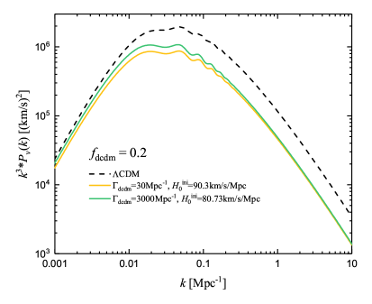
Therefore, a better choice (as in Ref. [35, 37]) is to fix the following cosmological parameters at the early time of same as those in standard CDM universe, including the baryon density , the total DM density , the amplitude of primordial perturbation , the index of the primordial perturbation spectrum , the redshift of reionization and the angular size of the sound horizon . We also assume that the decaying DM of the density starts to decay at . With these parameters fixed and varying and , as the consequence, the present-day value of DM density , the optical depth and the Hubble constant will change accordingly. These fixed parameters are chosen from Planck 2015 best-fitted TT, TE, EE+Low-P parameters [1]: {, , , , , and }. To avoid confusions, hereinafter we abbreviate , and km/s/Mpc as the input/initial parameters. Note that, the angular size of the sound horizon is fixed in this section such that the peak positions of CMB TT spectrum are unaltered, which is convenient for our discussions and can cancel the trivial effects in the CMB [37]. When performing the Monte-Carlo analysis in Sec. 4, we of course leave as a parameter. For illustration purpose, we fix the fraction of decaying DM to be and the fiducial decay rate 111To be consistent with the units used in CAMB, the decay rate in this study is expressed in units of , related to other works making use of by the conversion factor of in the range of – Mpc-1. The evolution equations are numerically solved by a modified CAMB [71] code.
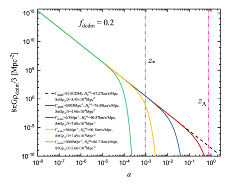
In Fig. 1, we illustrate the evolution of the background DCDM density evolution, starting with our initial conditions. We observe that, for the long-lived DCDM where Mpc-1 (i.e., longer than recombination time), the evolution starts to deviate from the standard CDM one when , which would lead to different predictions for , and be able to mitigate their tensions from recent cosmological data. For very large ( Mpc-1), corresponding to very short-lived DCDM, the DCDM density decreases significantly well before recombination (), leaving strong imprints on the CMB.
In all cases, eventually become smaller than its initial value due to the DCDM decay so that is automatically adjusted to higher values in order to keep the angular size fixed, in which is the sound horizon before photon decoupling and is the angular diameter distance to the last scattering surface. As a result, (or equivalently the density ) has to be changed and depend on non-monotonically when varying the decay rate. See more details and discussions in Appendix A.
3.2 Impacts on the CMB TT spectrum from DM decay


In this subsection we investigate the impacts of the decay on the CMB TT angular power spectrum. In order to fully understand the changes in CMB power spectrum, we will carefully examine the decay-induced impacts on the Sachs-Wolfe effect (SW), the early Integrated Sachs-Wolfe effect (early-ISW) and the late Integrated Sachs-Wolfe effect (late-ISW), as well as on the gravitational potential.
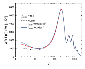
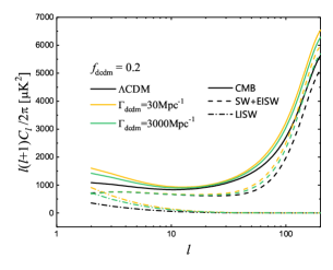
Let us first focus on the long-lived DCDM models where Mpc-1. From Fig. 2a, the amplitudes of the power spectrum at are almost identical for the different , but the decay apparently increases the amplitude at low- regime, .
These features are consistent with what we expect in the long-lived case from Fig. 1, since the DM lifetime longer than the recombination time would be almost no effect in the early universe but change the late universe considerably. The CMB perturbation modes at small scales with have already well entered the horizon after recombination, so that the decay is not able to affect those modes. As we fix in this section and decay will lead to a decrease in , the density has to be adjusted to a higher value when decay occurs (see Appendix A in detail). This process will always compensate for decreasing by increasing . As a result, a higher value of can lead to an enhancement in the ISW effect and consequently in low- CMB amplitudes.
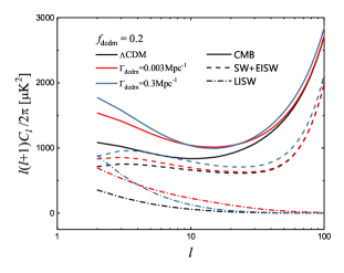
The enhancement in low- amplitude in fact comes from the decay-induced changes in the SW, early-ISW and late-ISW effects, which is shown in Fig. 2b. Let us focus on two cases: Mpc-1 and Mpc-1, respectively. We find that, the decay will increase the both SW and early-ISW effects at and the larger decay rate increase the total amplitude of the SW and early-ISW more than from the smaller one, whereas the increase in the late-ISW from the smaller one could be greater than that from the larger one, except for at very large scales of where the contribution to late-ISW is mainly from incerasing (i.e., increasing in order to keep fixed).
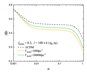
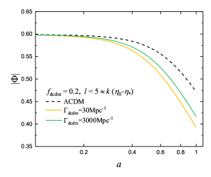
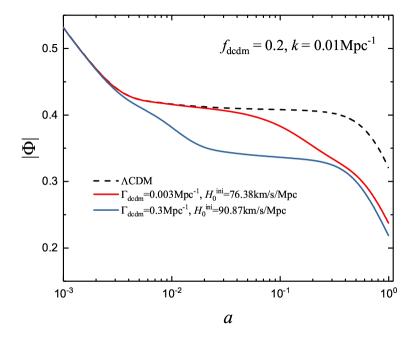
In order to physically understand these observed behaviors, we will investigate the evolution of the gravitational potential, namely the Weyl potential defined in CAMB, where the scalar metric perturbations evaluated in the Newtonian gauge are shown in Table 1. Intuitively due to the fact that the decay will decrease , we expect the growth of would be suppressed. As known, the SW and ISW effects are determined by the evolution of time-dependent gravitational potential. In Fig. 3, we illustrate the potential for given wavenumbers as a function of scalar factor . The wavenumber is related to the multipole through the relation of , where and denote the conformal time at the recombination and present day, respectively. As seen, compared with the standard CDM case, the smaller decay rate Mpc-1 mainly affect the potential at and the larger rate Mpc-1 affects earlier. Such influences increase the changes of after recombination, leading to a strong boost in the SW and ISW effects. Moreover, in Fig. 2b, the larger decay rate Mpc-1 can offer a strong SW and early-ISW effects at . For the late-ISW effect at in Fig. 2b, the potential decay at in DCDM model is stronger than that in the standard CDM model (seen from Fig. 3b) and the potential become lower for a larger , as expected.
From the above discussion about the case of the small decay rate, we are convinced that, the long-lived DCDM has almost no effect in the TT power spectrum at whereas it increases the amplitude of the spectrum notably at very large scales of . Note that, again, the angular size under the different decay rates is fixed to the value derived from the standard CDM model in the calculations, and therefore the density has to be adjusted accordingly.
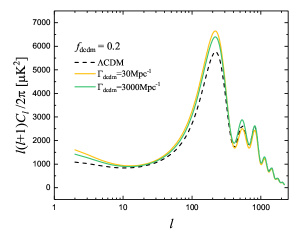
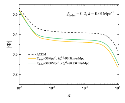
Next, let us move to the short-lived case which has a large decay rate with Mpc-1. As expected, the short-lived DCDM would play an important role at early universe before recombination, and leads to considerable changes in the CMB power spectrum at a broad range of multipoles, , shown in Fig. 4. To understand these features, following the same line of reasoning as in small case, Fig. 4b and 5 show the SW and the early/late-ISW effects, and the evolution of , respectively. As seen, due to the decay of DM which leads a suppression in , both the SW and ISW effects are enhanced visibly at the scales of . However, contrary to an intuitive expectation that the changes in from smaller decay rates are weaker than from larger ones, the smaller decay rate in fact will lead to a stronger influence in the CMB power spectrum. Also, all of the decaying DM with such large decay rates will disappear into dark radiations before the recombination and thus the comoving density of the remaining cold DM is unchanged with respect to , so that different decay rates will start to change differently, mostly at the very early universe at . Meanwhile, the detailed calculation in Appendix. B shows the anti-correlation between and in the short-lived case. This anti-correlated feature will be also related to the explanations of the results in Sec. 3.3 and 3.4.
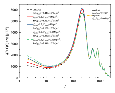
Now let us focus on the effects from the DM density fraction . Since the DM density in terms of the Taylor series of can be written as , the impacts on cosmological observables at the linear level are expected to depend on the quantity only, which means that the cosmological data could not break this degeneracy between and when and cosmological parameters are fixed. Nevertheless, the condition () can be relaxed for a specific cosmological probe. For example, from Fig. 2(a) we can observe that, changes on TT spectrum at by varying from 0.003 to 0.3 Mpc-1 with respect to the CDM one are almost negligible. This negligible effect is also observed at the EE power spectrum in Fig. 1 (Ref. [37]). Thus, the condition can be relaxed to Mpc-1 for the CMB signals at small scales, since we have fixed the (leading to adjusted accordingly for a given ) and the primary CMB acoustic peaks are then insensitive to the . Morever, as observed in Fig. 6, when is fixed in either long-lived or short-lived case, the changes in TT spectrum at are essentially invisible by varying . However, such strong degeneracy is entirely broken at the large scales since in our calculations is fixed and thus is changed accordingly by varying . The short-lived one can have an additional impact on the TT spectrum, boosting the first-peak amplitude, which might be due to contributions from the higher order terms .
For the sake of simplicity, here we only discuss the effects in the CMB TT power spectrum. It is straightforward to extend the discussion into CMB polarization patterns (for details of impacts on the polarization see Ref. [37]). However, when performing the joint analysis in Sec. 4, all Planck CMB power spectra of TT, TE and EE are included.
3.3 Impacts of DM decay on the growth of the large-scale structure
| z | Reference | |
|---|---|---|
| 0.02 | 0.360 0.040 | [75] |
| 0.067 | 0.423 0.055 | [76] |
| 0.10 | 0.37 0.13 | [77] |
| 0.17 | 0.51 0.06 | [78] |
| 0.22 | 0.42 0.07 | [79] |
| 0.38 | 0.497 0.045 | [80] |
| 0.41 | 0.45 0.04 | [79] |
| 0.51 | 0.458 0.038 | [80] |
| 0.6 | 0.43 0.04 | [79] |
| 0.61 | 0.436 0.034 | [80] |
| 0.77 | 0.490 0.180 | [78] |
| 0.78 | 0.38 0.04 | [79] |
| 0.80 | 0.47 0.08 | [81] |

A measurement of the large-scale structure growth may give further constraints on the DCDM model. In this study, we focus on the investigation of decay effects in the RSD and provide a constraint on the model by using the data (listed in Table 2) from [50]. The model independent matter growth rate is defined as
| (3.1) |
which in generally is a function of the redshift , however the growth rate might be not sensitive to the small scales of Mpc-1. In the DCDM model, the overdensity of total matter is modified as
| (3.2) |
where .
We usually use the variance of the density field smoothed within Mpc (denoted as or ) and the velocity-density correlation with the same smoothing scale , to estimate the growth rate through
| (3.3) |
There is no modification in the formalism of from the DCDM model in the synchronous gauge (see Eq. 2.3), so we have
| (3.4) |
which is completely different from interacting dark matter-dark energy scenarios [50, 72, 73, 74], and thus the measurements of from Eqs. 3.1 and 3.3 should be almost identical at small scales, confirmed by the illustration in Fig. 7.
For data, the measurements are based on the coherent motion of galaxies that characterized by the continuity equation, which reads
| (3.5) |
Here we have introduced the RSD parameter , with , where is the galaxy bias (). Under the assumption of , we can therefore straightly obtain the continuity equation for the total matter by combining Eq. 3.1 and Eq. 3.4 as
| (3.6) |
which indicates the strong dependence of the divergence of the velocity field on the growth rate.
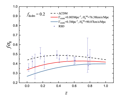
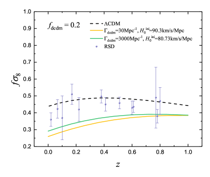
We now investigate the evolution of in the presence of the decaying DM. By varying the decay rate, Fig. 8 shows the predicted , together with the observational data. As seen, for long-lived DCDM will decrease as decreases monotonically, whereas for short-lived DCDM the anti-correlated feature (mentioned in Sec. 3.2) still exists, which is consistent with the impact of the decay on shown in Fig. 11 (see further discussion later).
Moreover, one may invoke the DCDM model, since the prediction on from CDM is slightly higher than the observed data222For example, the of for CDM and the DCDM model with Mpc-1 (the red line in Fig. 8a) are 28.07 and 11.51, respectively, implying the DCDM model have a better fit to observational growth rate data points with respect to the CDM one. and such overestimate can be reduced by allowing for our DCDM model that suppresses the growth rate of cosmological perturbations. Also, the in the low-z region () is very sensitive to the value of , and thus we expect that the current and the future data combined with the Planck CMB observations will provide a tight constraint on the decaying model.
3.4 Impacts of DM decay on baryon velocity field and kSZ effect
The baryon velocity field is an accurate tracer of the cosmic evolution that is sensitive to the DM decay, and thus it may pose a strong constraint for the DCDM model.
In the linear perturbation theory, the evolution of the baryon peculiar velocity in the Fourier space follows
| (3.7) |
where the subscript “b” represents baryon. The corresponding statistical information on can be obtained by translating into the root-mean-square velocity dispersion of baryon
| (3.8) |
within a sphere of radius , where is the power spectrum of , is the top-hat filter in the -space, and is the bulk flow of baryon on such radius .
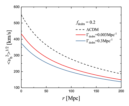
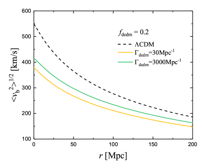
Fig. 9 illustrates a strong suppression in the baryon velocity field across all scales. A larger decay rate will lead to a stronger suppression for the long-lived DM model with Mpc-1. However, the short-lived DM impacts on the velocity field in the other way around and a larger decay rate will weaken the suppression from Fig. 9b. The trend of the suppression can be clearly understood as follows: 1) the top-hat filter in Eq. 3.8 results in the contribution of to almost from the modes with Mpc-1; 2) on very large scale is insignificant, and what really makes sense is the statistical information within range we plot in Fig. 10; 3) is the auto-correlation of , and on small scales the baryon velocity field is proportional to the overdensity that is still controlled by the gravitational potential. The deeper the potential is, the stronger the resulting growth is, which is demonstrated by varying the decay rates shown in Fig. 11.

Furthermore, we also expect that the decaying DM would affect the velocity field of the universe even before the reionization, which might be able to be tested by the kinetic Sunyaev-Zel’dovich effect (kSZ) that directly encode the information of the peculiar velocity field of the matter distribution and the baryonic matter density. The kSZ induced temperature anisotropies in a given direction () on the sky is given by [82]
| (3.9) |
where is the electron density, the Thomson cross-section, the optical depth, the peculiar velocity vector of ionized electrons and corresponds to the distance along the line-of-sight (l.o.s) from , which will happen before the reionization as we want to collect all the kSZ signals along l.o.s, to the present day . Assuming , where is the ionization fraction, the mean electron density today and is the position in comoving coordinates. For simplicity, in this study we only consider the contribution from homogenous kSZ, not from the patchy effect. The “patchy” reionization kSZ in the fiduical model is subdominant with respect to the homogeneous one. Also, the patchy effect is stronly model dependent and depends on . Moreover, one could separate the late-time and reionization kSZ by considering a higher-order statistic proposed in Ref. [83]. With this concern, in this study is assumed to be a function of the redshift only, and the contribution from inhomogeneous is neglected. The kSZ-induced temperature anisotropies then can be computed as
| (3.10) |
in which is the peculiar momentum of the free electrons and can be decomposed into the gradient part and the curl part . As known, there is no contribution from to the kSZ effect [84, 85] since the gradient part cancels out when integrating along the line of sight. Thus we only consider the curl part and the corresponding power spectrum is computed by
| (3.11) |
where is the power spectrum of and the kernel . In the linear perturbation theory and for , the peculiar velocity is related to the overdensity through
| (3.12) |
in which is the growth factor for the electron overdensity that is same as the baryonic one at the linear level. With by setting , Eq. 3.11 can be re-expressed as
| (3.13) |
where is the linear power spectrum of the baryon, is the transfer function that suppresses the at small scales [86] and we take it as unity in our calculations. Since the non-linear evolution of matter overdensity would enhance the kSZ signal, this effect can be modeled by a transfer function such that the non-linear power spectrum . Refering to Ref. [87, 88, 89], one can recast Eq. 3.13 for the non-linear effect as
| (3.14) |
In non-standard cosmology, can be accurately fitted from numerical simulations. Several works dedicated to non-linear clustering [37, 69] find that the standard Halofit model would significantly overestimate the small-scale power spectrum in the presence of the DCDM models [90, 91]. Recently, Ref. [69] provides a more accurate fitting formula from N-body simulations to correct such overestimation. However, this fitting formula is guaranteed to be accurate only for the extreme long-lived DCDM model of GyrMpc, which has a much longer lifetime than the typical values of investigated in this study. With a conservative assumption that the predicted value from this fitting formula for a larger would not be deviated considerably, we therefore calculate the non-linear growth of the baryon via the fitting formula evaluated by a fixed of Gyr-1. The kSZ signal thus can be calculated through
| (3.15) |
where . The contribution to kSZ signal from high redshifts is quite small since in the fiducial “sudden” reionization model used in CAMB [92] with and , where is the redshift when the reionization fraction is about half of its maximum and is the width of the reionization transition. From numerical tests, we choose the upper limit of the integral as as any contributions from the higher ones can be safely neglected.
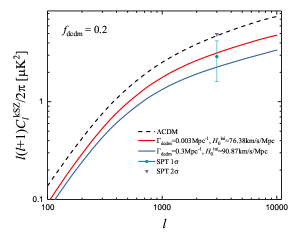
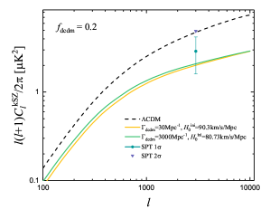
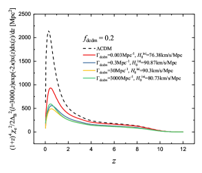
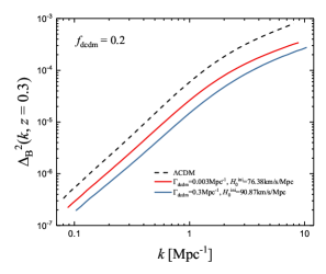
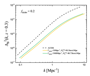
Fig. 12 shows the predicted angular power spectrum of the kSZ anisotropies in the presence of the DCDM, in comparison with the measured data from the South Pole Telescope (SPT) [93]. The measured amplitude of the kSZ power spectrum by SPT is at and the corresponding upper limit is about . As seen, the predicted amplitude of kSZ from the standard CDM is consistent within measured value at the level, whereas the current measurement in fact favour the DCDM model as the kSZ signal will be suppressed considerably by the presence of the DCDM which leads to the kSZ amplitudes consistent with data within . Furthermore, the DCDM-induced influences in kSZ for the long-lived (in Fig. 12a) and short-lived (in Fig. 12b) models are essentially compatible with those in the bulk flow of the baryon shown in Fig. 9.
In Fig. 13a, we illustrate the integrand in Eq. 3.15 as the function of at . One can find that the dominated contributions to the kSZ power spectrum only come from low redshifts of , which means the kSZ signal is not strongly dependent on the reionization history. Again, is fixed in calculating the kSZ signals for different decay rates. With such “fixing”, changing the decay rate will lead to a different dark energy density and Hubble expansion rate, and, consequently, leave an impact on and in Eq. 3.15. Furthermore, as shown in Fig. 13b, the power spectrum will decrease monotonically as increasing in the long-lived case. From Fig. 13c, we also find that a strong suppression in appears whereas the strength of such suppression is insensitive to in the short-lived case.
With the above discussions about the DCDM-induced suppression in the kSZ power spectrum, the recent kSZ measurement by SPT would provide a further constraint on the parameter space of the DCDM model and MCMC-based constraints by using current observations are present in Sec. 4.
4 Constraints on DM decay rate and fraction
In this section, by running Monte Carlo Markov chains (MCMC) with using the public code CosmoMC [94, 95], we perform a joint analysis of the cosmological data to place tight constraints on the DCDM model. We compare the constraining power of various observables including the CMB, BAO, RSD and kSZ measurements as follows.
4.1 Constraints from the CMB power spectra, BAO and data
To understand how the measurements improve the constrains on the DCDM model, we start with using Planck 2015 temperature and polarization data over the full range of multipoles (referring to them as “Planck2015”) 333The CMB data used in the analysis include the Planck low- () TT, TE, EE spectra, combined with the high- data in the range of for TT and for TE and EE.. We then include the data listed in Tab. 2 and refer to these data as “RSD” 444Compared with Ref. [38], in this study we further take into account the decay before the recombination and perform an analysis with more RSD data involved.. After that, we add BAO data from Six-degree-Field Galaxy Survey (6DFGS) at [96], SDSS Main Galaxy Sample (MGS) at [97], the BOSS-LOWZ at effective redshift and the CMASS-DR11 at effective redshift [98], for placing further constraints on the DCDM model. In our analysis, we assume flat priors on the six cosmological parameters and two DCDM-related ones: . Note that, we choose a flat prior on as Mpc-1 for the long-lived case and Mpc for the short-lived one. We also keep the total neutrino mass, the relativistic number of degrees of freedom and the spectrum lensing normalization as well as the Helium fraction fixed to eV, , and , respectively. We set a Gelman and Rubin criterion of to ensure the chains to be converged.
| Planck2015+BAO | Planck2015+BAO+RSD | |||
| Parameter | Best fit | 68% limits | Best fit | 68% limits |
| 0.02233 | 0.02223 | |||
| 0.1189 | 0.1198 | |||
| 1.041 | 1.041 | |||
| 0.09105 | 0.07504 | |||
| 0.9655 | 0.9635 | |||
| 3.114 | 3.084 | |||
| Mpc-1 | ||||
| 0.001585 | 0.008991 | |||
| 0.6917 | 0.6933 | |||
| 0.3083 | 0.3067 | |||
| 11.09 | 9.7 | |||
| 67.83 | 68.21 | |||
| 0.836 | 0.8251 | |||
| 13.79 | 13.77 | |||


| Planck2015+BAO | Planck2015+BAO+RSD | |||
|---|---|---|---|---|
| Parameter | Best fit | 68% limits | Best fit | 68% limits |
| 0.02224 | 0.02216 | |||
| 0.1299 | 0.1213 | |||
| 1.041 | 1.041 | |||
| 0.08943 | 0.05536 | |||
| 0.9787 | 0.9696 | |||
| 3.128 | 3.052 | |||
| Mpc | 2.365 | 2.043 | ||
| 0.05596 | 0.01446 | |||
| 0.6741 | 0.6874 | |||
| 0.3259 | 0.3126 | |||
| 11.08 | 7.832 | |||
| 68.46 | 67.91 | |||
| 0.8657 | 0.8167 | |||
| 13.68 | 13.78 | |||

In Fig. 14, we first consider the models of CDM and DCDM constrained by “Planck2015” and RSD data, respectively. We see that, the inferred values of and from CMB data are still in about tensions with those from RSD data and the DCDM model can only slightly alleviate such tensions, which confirms the results found in Ref. [37]. Then in Table. 3, we present the results for the long-lived DCDM model from the combined datasets “Planck15+BAO” and “Planck15+BAO+RSD”, and the inferred 1D distributions and 2D contours are shown in Fig. 15.
Using the “Planck15+BAO” dataset, we find a CL upper limits on the fraction is but very weak constraint on due to the tiny changes from the decay in the CMB angular power spectra at (see Fig. 2a and Fig. 1 in Ref. [37]). When including RSD data in the analysis, one can not obtain stronger constraint on , and the bound on now becomes weaker by about a factor of 1.1. These results indicate that the RSD data prefer a relatively larger decaying DM fraction, consistent with our findings in Sec. 3.3 where the predicted values of fit the data better than the CDM predicted. Also, as expected, the current datasets can not effectively break down the degeneracy between and for the long-lived model (see Fig. 6).
The constraints in the short-lived DCDM model (most of the DCDM has decayed away before the recombination) are summarized in Tab. 4 and the corresponding 1D marginalized posterior distributions and 2D contours are shown in Fig. 16. To speed up the exploration of the parameter space in , we scan over Mpc with a flat prior instead of . Due to the fact that the total DM density at the recombination is tightly fixed by the CMB and increasing will lead to the total DM density significantly decreased at that time, therefore one can find a strong positive correlation between initial DM density and DM fraction . From the 1D distributions, we also find that, the RSD data provides strong constraints on and and the bound on , however, becomes slightly weaker than that by “Planck2015+BAO”. As known from Fig. 8b, the predicted from the short-lived case is noticeably lower than the CDM one, and thus the current RSD data obtained from the surveys in late universe are much more in favor of the lower abundance of DCDM. Furthermore, Fig. 8b also indicates that for a fixed the larger leads to a smaller suppression on and gives a better fit to the data. As a result, a lower abundance of DCDM with a relatively larger decay rate would be also compatible with the data “Planck2015+BAO+RSD”, which gives rise to a relatively weaker bound on with the inclusion of RSD data. Finally, the marginalized upper limit on is improved by a factor of about 1.9 ( from “Planck2015+BAO” and from “Planck2015+BAO+RSD”), when the RSD data are included in the analysis.
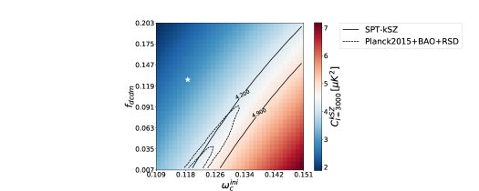
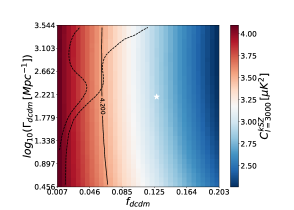
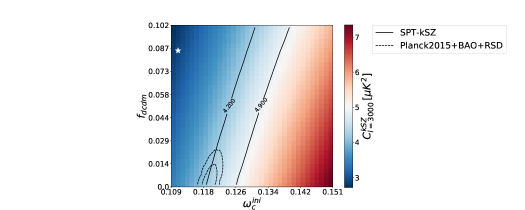
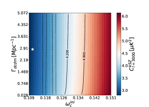
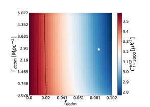
4.2 Adding kSZ data from SPT
The influences of DM decays on the kSZ signal has been investigated in Sec. 3.4, and thus let us compute the constraining power of the SPT-kSZ data. Since the SPT provides a measurement of the kSZ signal at only, it is not able to provide significant improvements in the constraints on the DCDM model. Here, we therefore only investigate the constraint from such kSZ data by fixing cosmological parameters with the “Planck 2015” best-fitted values but varying , and that allows us to construct a 3D parameter space. In Fig. 17 and 18, we show the results for the long- and short-lived DCDM models, respectively. Comparing with the constraining power of the “Planck2015+BAO+RSD” dataset, the current kSZ data prefers a non-zero fraction of DCDM, which is consistent with the results in Sec. 3.4 but somewhat opposite to the preference from “CMB+BAO+RSD” measurements. We find that the best fitted value of the SPT-kSZ measurement (the “white star” in Fig. 17 & 18) deviates from the “Planck2015+BAO+RSD”-inferred one at 2 level. This disagreement might imply a possible tension between the current kSZ and CMB data, and future precise kSZ measurements would provide independent evidence for the existence of DCDM.

5 Conclusions
In this work, we have investigated cosmological bounds on a fractional decaying DM that is allowed to decay into invisible relativistic particles (“dark radiation”). The DCDM model is characterized by two parameters, the fraction of the DCDM and the decay width , and we estimate the constraints on such two parameters by purely gravitational effects from the measurements of the CMB temperature anisotropies, the redshift distortion and the kinetic Sunyaev-Zel’dovich effect. Based on a full calculation of the evolution equations for the background and the perturbations by modifying the full Boltzmann hierarchy, we have quantitatively determined the impacts of the decaying DM on cosmological observables and placed a cosmological constrains on and from a joint analysis of the cosmological data by running Monte Carlo Markov chains.
With respect to the previous literature, the main features of this paper are as follows. 1) More cosmological observables have been taken into account in the analysis, including not only the CMB temperature anisotropies, but also the structure growth rate, the bulk flow of the baryon and the kSZ effect. 2) We have evaluated in detail the impacts of the DM decay on the Sachs-Wolfe (SW) effect, the early/late Integrated SW effects, as well as on the evolution of the Weyl potential , which explicitly provides physical explanations for the decay-induced signatures in the CMB TT power spectrum, the growth rate , the bulk flow of baryon , and the kSZ power spectrum. We find that the DM decay leads to a visible suppression in and consequently changes the above-mentioned cosmological observables accordingly. 3) When adding growth rate measurements of the RSD data, the CL upper limit tightens considerably from to for the short-lived DCDM model, whereas the inclusion of RSD data can not place a tighter constraint on than that from the combined dataset of “CMB+BAO” for the long-lived one. our results also show that the DCDM model does not significantly alleviate the and tensions, which remain at 3 level. 4) For the first time, we also investigated the constraining power of the kSZ effect on the DCDM model in detail. The current SPT-kSZ prefers the presence of the decaying DM that leads to a suppression in the kSZ power spectrum. The derived contours from the kSZ data alone, which are different from the “CMB+BAO+RSD” inferred ones, indicate that the kSZ signal is sensitive to the DCDM model and would provide an independent constraint on the parameter space. We thus expect that future precise kSZ surveys will constrain the properties of DCDM tightly.
Definitely, if the cold DM decays into electromagnetic particles, many other cosmological observables will provide additional information for detecting/constraining the decaying DM, such as the reionization history (e.g., [99, 100, 101]), and, the existence of DCDM can be strictly tested by ongoing and future reionization observations [102, 103, 104, 105, 106, 107, 108, 109]. Moreover, the weak lensing surveys [110, 111, 112, 113] are expected to further improve the constraints considerably. Finally, it is worthwhile to examine the impacts of DCDM models on the non-linear clustering regime carefully by N-body simulations in a future study.
Appendix A Adjust the initial and for keeping fixed
When investigating and discussing the new physics using cosmological observations, one has to specify which cosmological parameters are kept fixed, in order to clearly demonstrate predicted signatures from new physics.
Specifically, the effects of DM decay rate on the CMB can lead to a change in the angular diameter distance to decoupling and a shift of the peaks and trough positions, compared with the standard CDM predictions. To cancel the trivial effects in the CMB and to discuss the effects associated to the decays conveniently, we keep a constant value of for the DCDM model before Sec. 4 and, consequently, the initial Hubble parameter and will be adjusted accordingly for a given and . Note that, we however treat as a free parameter for the MCMC analysis in Sec. 4.
Now, let us focus on the dependence of and on when fixing . By definition,
| (A.1) |
where
| (A.2) | |||
| (A.3) |
Here, and denote the sound horizon before the photon decoupling at and the angular diameter distance from last scattering surface to us, respectively. is the speed of sound in the photon-baryon fluid. As expected, the decay will change the Hubble expansion rate due to some amount of DM () decaying into invisible relativistic particles (), and then alter the . By assuming the present-day value of the baryon density is fixed, varying the dark energy density gives a solution for compensating for the change in .
For the long-lived model, as the typical time scale of the decay , the is insensitive to the decay, but the would increase significantly due to a large decrease in . We therefore increase to reduce the so as to keep unchanged. Moreover, the larger will enhance the CMB low- power due to the late integrated Sachs-Wolfe effect.
For the short-lived model where Mpc-1, the typical decay occurs before the recombination and only a small fraction of decaying DM are still alive at the late-time universe. In this scenario, the decay has impacts on both and , unlike the long-lived model. Increasing will lead to both and increased as decreased. However, , the ratio of and , does not monotonically change in , since the dependences of and on are obviously different. As a result, in some cases with considerably large , the changes in would become even smaller than those from a smaller (shown in Fig. 1).
In Tab. 5, we illustrate the derived values of , and by varying and , while keeping fixed. For each , with adjusting to an appropriate value or without, we clearly demonstrate the effects of the decay in . When fixing to the standard value (i.e., ), we qualitatively confirm the above claims. One can find that, the increase in for Mpc-1 (i.e., short-lived) is smaller than that for or 30 Mpc-1, and must be adjusted to the higher values (increased by 42.2 and by for and Mpc-1 for the long-lived model, respectively.
| Mpc-1 | Mpc-1 | Mpc-1 | ||
|---|---|---|---|---|
| 0 | 1 | 144.551 | 13889.245 | 1 |
| 0.003 | 1.422 | 144.551 | 13888.883 | 1 |
| 0.003 | 1 | 144.551 | 14274.113 | 0.973 |
| 0.3 | 2.205 | 144.580 | 13891.647 | 1 |
| 0.3 | 1 | 144.580 | 14847.220 | 0.935 |
| 30 | 2.171 | 146.391 | 14065.403 | 1 |
| 30 | 1 | 146.391 | 15002.749 | 0.937 |
| 3000 | 1.643 | 150.297 | 14441.074 | 1 |
| 3000 | 1 | 150.297 | 15019.707 | 0.961 |
Appendix B Behaviours of on large
Here, we apply for a semi-analytical method to qualitatively understand the behaviours of on large mentioned in Sec. 3.2, where a larger however leads to a smaller suppression in , completely different from what we would expect.
For simplicity (without loss of generality), suppose that , Eqs. 2.1 and 2.2 then reads
| (B.1) | |||||
| (B.2) |
The analytic solutions of these two equations are expressed by
| (B.3) | |||||
| (B.4) |
where is the proper time and the (’) denotes integration variables. The Weyl potential is determined by the Poisson equation,
| (B.5) |
in which and collect all the linear terms in perturbations (e.g., overdensity, peculiar velocity, etc.), and and .
Recalling the adopted initial condition described in Sec. 3.1, and defining , the deviation of from the , one can explicitly rewrite Eq. B.5 as
| (B.6) |
Here, we have assumed that, before the matter-dominated epoch there is no difference in or between the CDM and the DCDM model. During the radiation dominated epoch (RD), Mpc when and Mpc when , so that . With this approximation, one can further derive the following equation,
| (B.7) |
As known that during RD in the CDM, is expected be positive. If is small enough, , implying that the evolution of is well consistent with that in the CDM. Now, let us move to the short-lived scenario with a very large (e.g., Mpc-1 in Fig. 5). At the RD (), Eq. B.7 indicates the value of in the DCDM model tends to be larger than that in the CDM, and a larger will lead to a larger (i.e., ). However, at the epoch after the recombination (), all decaying DM completely decay away for such large decay rates (i.e., ), giving rise to . Along with the cosmological evolution, the trend of is still observed from our numerical calculations, leading to the feature of the deeper suppression for the smaller shown in Fig. 5.
Acknowledgments
This work was supported by the National Science Foundation of China (11621303, 11653003, 11773021, 11835009,11890691), the National Key R&D Program of China (2018YFA0404601, 2018YFA0404504), the 111 project, and the CAS Interdisciplinary Innovation Team (JCTD-2019-05).
References
- [1] P. A. R. Ade et al. [Planck Collaboration], “Planck 2015 results. XIII. Cosmological parameters,” Astron. Astrophys. 594, A13 (2016), arXiv:1502.01589 [astro-ph.CO].
- [2] N. Aghanim et al. [Planck Collaboration], “Planck 2018 results. VI. Cosmological parameters,” arXiv:1807.06209 [astro-ph.CO].
- [3] A. G. Riess et al., “A 3% Solution: Determination of the Hubble Constant with the Hubble Space Telescope and Wide Field Camera 3,” Erratum: [Astrophys. J. 732, 129 (2011)], arXiv:1103.2976 [astro-ph.CO].
- [4] A. G. Riess et al., “A 2.4% Determination of the Local Value of the Hubble Constant,” Astrophys. J. 826, no. 1, 56 (2016), arXiv:1604.01424 [astro-ph.CO].
- [5] J. Hamann and J. Hasenkamp, “A new life for sterile neutrinos: resolving inconsistencies using hot dark matter,” JCAP 1310, 044 (2013), arXiv:1308.3255 [astro-ph.CO].
- [6] R. A. Battye and A. Moss, “Evidence for Massive Neutrinos from Cosmic Microwave Background and Lensing Observations,” Phys. Rev. Lett. 112, no. 5, 051303 (2014), arXiv:1308.5870 [astro-ph.CO].
- [7] A. Petri, J. Liu, Z. Haiman, M. May, L. Hui and J. M. Kratochvil, “Emulating the CFHTLenS Weak Lensing data: Cosmological Constraints from moments and Minkowski functionals,” Phys. Rev. D 91, no. 10, 103511 (2015), arXiv:1503.06214 [astro-ph.CO].
- [8] A. A. Klypin, A. V. Kravtsov, O. Valenzuela and F. Prada, “Where are the missing Galactic satellites?,” Astrophys. J. 522, 82 (1999), [astro-ph/9901240].
- [9] J. D. Simon and M. Geha, “The Kinematics of the Ultra-Faint Milky Way Satellites: Solving the Missing Satellite Problem,” Astrophys. J. 670, 313 (2007), arXiv:0706.0516 [astro-ph].
- [10] S. Weinberg, “The Cosmological Constant Problem,” Rev. Mod. Phys. 61, 1 (1989).
- [11] L. P. Chimento, A. S. Jakubi, D. Pavon and W. Zimdahl, “Interacting quintessence solution to the coincidence problem,” Phys. Rev. D 67, 083513 (2003), [astro-ph/0303145].
- [12] R. Y. Guo, J. F. Zhang and X. Zhang, “Can the tension be resolved in extensions to CDM cosmology?,” JCAP 1902, 054 (2019), arXiv:1809.02340 [astro-ph.CO].
- [13] S. Kumar, R. C. Nunes and S. K. Yadav, “Dark sector interaction: a remedy of the tensions between CMB and LSS data,” arXiv:1903.04865 [astro-ph.CO].
- [14] H. Miao and Z. Huang, “The Tension in Non-flat QCDM Cosmology,” Astrophys. J. 868, no. 1, 20 (2018), arXiv:1803.07320 [astro-ph.CO].
- [15] E. Mörtsell and S. Dhawan, “Does the Hubble constant tension call for new physics?,” JCAP 1809, no. 09, 025 (2018), arXiv:1801.07260 [astro-ph.CO].
- [16] V. Poulin, T. L. Smith, T. Karwal and M. Kamionkowski, “Early Dark Energy Can Resolve The Hubble Tension,” arXiv:1811.04083 [astro-ph.CO].
- [17] S. Vagnozzi, “New physics in light of the tension: an alternative view,” arXiv:1907.07569 [astro-ph.CO].
- [18] M. A. Buen-Abad, R. Emami and M. Schmaltz, “Cannibal Dark Matter and Large Scale Structure,” Phys. Rev. D 98, no. 8, 083517 (2018), arXiv:1803.08062 [hep-ph].
- [19] M. Raveri, W. Hu, T. Hoffman and L. T. Wang, “Partially Acoustic Dark Matter Cosmology and Cosmological Constraints,” Phys. Rev. D 96, no. 10, 103501 (2017), arXiv:1709.04877 [astro-ph.CO].
- [20] W. J. C. da Silva, H. S. Gimenes and R. Silva, “Extended CDM model,” Astropart. Phys. 105, 37 (2019), arXiv:1809.07797 [astro-ph.CO].
- [21] F. D’Eramo, R. Z. Ferreira, A. Notari and J. L. Bernal, “Hot Axions and the tension,” JCAP 1811, no. 11, 014 (2018), arXiv:1808.07430 [hep-ph].
- [22] P. Ko, N. Nagata and Y. Tang, “Hidden Charged Dark Matter and Chiral Dark Radiation,” Phys. Lett. B 773, 513 (2017), arXiv:1706.05605 [hep-ph].
- [23] A. G. Doroshkevich, M. Khlopov and A. A. Klypin, “Large-scale structure of the universe in unstable dark matter models,” Mon. Not. Roy. Astron. Soc. 239, 923 (1989).
- [24] M. Kaplinghat, R. E. Lopez, S. Dodelson and R. J. Scherrer, “Improved treatment of cosmic microwave background fluctuations induced by a late decaying massive neutrino,” Phys. Rev. D 60, 123508 (1999), [astro-ph/9907388].
- [25] K. Ichiki, M. Oguri and K. Takahashi, “WMAP constraints on decaying cold dark matter,” Phys. Rev. Lett. 93, 071302 (2004), [astro-ph/0403164].
- [26] M. Lattanzi and J. W. F. Valle, “Decaying warm dark matter and neutrino masses,” Phys. Rev. Lett. 99, 121301 (2007), arXiv:0705.2406 [astro-ph].
- [27] Y. Gong and X. Chen, “Cosmological Constraints on Invisible Decay of Dark Matter,” Phys. Rev. D 77, 103511 (2008), arXiv:0802.2296 [astro-ph].
- [28] S. De Lope Amigo, W. M. Y. Cheung, Z. Huang and S. P. Ng, “Cosmological Constraints on Decaying Dark Matter,” JCAP 0906, 005 (2009), arXiv:0812.4016 [hep-ph].
- [29] A. H. G. Peter, “Mapping the allowed parameter space for decaying dark matter models,” Phys. Rev. D 81, 083511 (2010), arXiv:1001.3870 [astro-ph.CO].
- [30] A. H. G. Peter and A. J. Benson, “Dark-matter decays and Milky Way satellite galaxies,” Phys. Rev. D 82, 123521 (2010), arXiv:1009.1912 [astro-ph.GA].
- [31] R. Huo, “Constraining Decaying Dark Matter,” Phys. Lett. B 701, 530 (2011), arXiv:1104.4094 [hep-ph].
- [32] S. Aoyama, K. Ichiki, D. Nitta and N. Sugiyama, “Formulation and constraints on decaying dark matter with finite mass daughter particles,” JCAP 1109, 025 (2011), arXiv:1106.1984 [astro-ph.CO].
- [33] M. Y. Wang, R. A. C. Croft, A. H. G. Peter, A. R. Zentner and C. W. Purcell, “Lyman-α forest constraints on decaying dark matter,” Phys. Rev. D 88, no. 12, 123515 (2013), arXiv:1309.7354 [astro-ph.CO].
- [34] S. Aoyama, T. Sekiguchi, K. Ichiki and N. Sugiyama, “Evolution of perturbations and cosmological constraints in decaying dark matter models with arbitrary decay mass products,” JCAP 1407, 021 (2014), arXiv:1402.2972 [astro-ph.CO].
- [35] B. Audren, J. Lesgourgues, G. Mangano, P. D. Serpico and T. Tram, “Strongest model-independent bound on the lifetime of Dark Matter,” JCAP 1412, no. 12, 028 (2014), arXiv:1407.2418 [astro-ph.CO].
- [36] A. Chudaykin, D. Gorbunov and I. Tkachev, “Dark matter component decaying after recombination: Lensing constraints with Planck data,” Phys. Rev. D 94, 023528 (2016), arXiv:1602.08121 [astro-ph.CO].
- [37] V. Poulin, P. D. Serpico and J. Lesgourgues, “A fresh look at linear cosmological constraints on a decaying dark matter component,” JCAP 1608, no. 08, 036 (2016), arXiv:1606.02073 [astro-ph.CO].
- [38] A. Chudaykin, D. Gorbunov and I. Tkachev, “Dark matter component decaying after recombination: Sensitivity to baryon acoustic oscillation and redshift space distortion probes,” Phys. Rev. D 97, no. 8, 083508 (2018), arXiv:1711.06738 [astro-ph.CO].
- [39] S. Tulin and H. B. Yu, “Dark Matter Self-interactions and Small Scale Structure,” Phys. Rept. 730, 1 (2018), arXiv:1705.02358 [hep-ph].
- [40] L. Amendola, “Coupled quintessence,” Phys. Rev. D 62, 043511 (2000), [astro-ph/9908023].
- [41] L. Amendola and C. Quercellini, “Tracking and coupled dark energy as seen by WMAP,” Phys. Rev. D 68, 023514 (2003), [astro-ph/0303228].
- [42] D. Pavon and W. Zimdahl, “Holographic dark energy and cosmic coincidence,” Phys. Lett. B 628, 206 (2005), [gr-qc/0505020].
- [43] C. G. Boehmer, G. Caldera-Cabral, R. Lazkoz and R. Maartens, “Dynamics of dark energy with a coupling to dark matter,” Phys. Rev. D 78, 023505 (2008), arXiv:0801.1565 [gr-qc].
- [44] G. Olivares, F. Atrio-Barandela and D. Pavon, “Matter density perturbations in interacting quintessence models,” Phys. Rev. D 74, 043521 (2006), [astro-ph/0607604].
- [45] O. Bertolami, F. Gil Pedro and M. Le Delliou, “Dark Energy-Dark Matter Interaction and the Violation of the Equivalence Principle from the Abell Cluster A586,” Phys. Lett. B 654, 165 (2007), astro-ph/0703462 [ASTRO-PH].
- [46] S. Micheletti, E. Abdalla and B. Wang, “A Field Theory Model for Dark Matter and Dark Energy in Interaction,” Phys. Rev. D 79, 123506 (2009), arXiv:0902.0318 [gr-qc].
- [47] L. Lopez Honorez, B. A. Reid, O. Mena, L. Verde and R. Jimenez, “Coupled dark matter-dark energy in light of near Universe observations,” JCAP 1009, 029 (2010), arXiv:1006.0877 [astro-ph.CO].
- [48] A. A. Costa, L. C. Olivari and E. Abdalla, “Quintessence with Yukawa Interaction,” Phys. Rev. D 92, no. 10, 103501 (2015), arXiv:1411.3660 [astro-ph.CO].
- [49] C. van de Bruck and J. Morrice, “Disformal couplings and the dark sector of the universe,” JCAP 1504, 036 (2015), arXiv:1501.03073 [gr-qc].
- [50] A. A. Costa, X. D. Xu, B. Wang and E. Abdalla, “Constraints on interacting dark energy models from Planck 2015 and redshift-space distortion data,” JCAP 1701, no. 01, 028 (2017), arXiv:1605.04138 [astro-ph.CO].
- [51] B. Wang, E. Abdalla, F. Atrio-Barandela and D. Pavon, “Dark Matter and Dark Energy Interactions: Theoretical Challenges, Cosmological Implications and Observational Signatures,” Rept. Prog. Phys. 79, no. 9, 096901 (2016), arXiv:1603.08299 [astro-ph.CO].
- [52] W. Yang, S. Pan, E. Di Valentino, R. C. Nunes, S. Vagnozzi and D. F. Mota, “Tale of stable interacting dark energy, observational signatures, and the tension,” JCAP 1809, 019 (2018), arXiv:1805.08252 [astro-ph.CO].
- [53] E. Di Valentino, A. Melchiorri, O. Mena and S. Vagnozzi, “Interacting dark energy after the latest Planck, DES, and measurements: an excellent solution to the and cosmic shear tensions,” arXiv:1908.04281 [astro-ph.CO].
- [54] A. De Felice and S. Tsujikawa, “f(R) theories,” Living Rev. Rel. 13, 3 (2010), arXiv:1002.4928 [gr-qc].
- [55] T. Harko and F. S. N. Lobo, “Generalized curvature-matter couplings in modified gravity,” Galaxies 2, no. 3, 410 (2014), arXiv:1407.2013 [gr-qc].
- [56] J. Preskill, M. B. Wise and F. Wilczek, “Cosmology of the Invisible Axion,” Phys. Lett. B 120, 127 (1983).
- [57] R. D. Peccei and H. R. Quinn, “CP Conservation in the Presence of Instantons,” Phys. Rev. Lett. 38, 1440 (1977).
- [58] H. Goldberg, “Constraint on the Photino Mass from Cosmology,” Erratum: [Phys. Rev. Lett. 103, 099905 (2009)].
- [59] G. Jungman, M. Kamionkowski and K. Griest, “Supersymmetric dark matter,” Phys. Rept. 267, 195 (1996), [hep-ph/9506380].
- [60] B. W. Lee and S. Weinberg, “Cosmological Lower Bound on Heavy Neutrino Masses,” Phys. Rev. Lett. 39, 165 (1977).
- [61] G. Servant and T. M. P. Tait, “Is the lightest Kaluza-Klein particle a viable dark matter candidate?,” Nucl. Phys. B 650, 391 (2003), [hep-ph/0206071].
- [62] H. C. Cheng, J. L. Feng and K. T. Matchev, “Kaluza-Klein dark matter,” Phys. Rev. Lett. 89, 211301 (2002), [hep-ph/0207125].
- [63] J. A. Adams, S. Sarkar and D. W. Sciama, “CMB anisotropy in the decaying neutrino cosmology,” Mon. Not. Roy. Astron. Soc. 301, 210 (1998), [astro-ph/9805108].
- [64] X. L. Chen and M. Kamionkowski, “Particle decays during the cosmic dark ages,” Phys. Rev. D 70 (2004) 043502, [astro-ph/0310473].
- [65] L. Zhang, X. Chen, M. Kamionkowski, Z. g. Si and Z. Zheng, “Constraints on radiative dark-matter decay from the cosmic microwave background,” Phys. Rev. D 76, 061301 (2007), arXiv:0704.2444 [astro-ph].
- [66] L. Zhang, X. L. Chen, Y. A. Lei and Z. G. Si, “The impacts of dark matter particle annihilation on recombination and the anisotropies of the cosmic microwave background,” Phys. Rev. D 74, 103519 (2006), [astro-ph/0603425].
- [67] K. L. Pandey, T. Karwal and S. Das, “Alleviating the and anomalies with a decaying dark matter model,” arXiv:1902.10636 [astro-ph.CO].
- [68] K. Vattis, S. M. Koushiappas and A. Loeb, “Late universe decaying dark matter can relieve the tension,” arXiv:1903.06220 [astro-ph.CO].
- [69] K. Enqvist, S. Nadathur, T. Sekiguchi and T. Takahashi, “Decaying dark matter and the tension in ,” JCAP 1509, no. 09, 067 (2015), arXiv:1505.05511 [astro-ph.CO].
- [70] C. P. Ma and E. Bertschinger, “Cosmological perturbation theory in the synchronous and conformal Newtonian gauges,” Astrophys. J. 455, 7 (1995), [astro-ph/9506072].
- [71] A. Lewis, A. Challinor and A. Lasenby, “Efficient computation of CMB anisotropies in closed FRW models,” Astrophys. J. 538, 473 (2000), [astro-ph/9911177].
- [72] R. J. F. Marcondes, R. C. G. Landim, A. A. Costa, B. Wang and E. Abdalla, “Analytic study of the effect of dark energy-dark matter interaction on the growth of structures,” JCAP 1612, no. 12, 009 (2016), arXiv:1605.05264 [astro-ph.CO].
- [73] R. An, A. A. Costa and B. Wang, “Constraints on the quintessence model with Yukawa interaction from Planck 2015 and weak lensing data,” arXiv:1809.03224 [astro-ph.CO].
- [74] A. A. Costa et al., “J-PAS: forecasts on interacting dark energy from baryon acoustic oscillations and redshift-space distortions,” arXiv:1901.02540 [astro-ph.CO].
- [75] M. J. Hudson and S. J. Turnbull, “The growth rate of cosmic structure from peculiar velocities at low and high redshifts,” Astrophys. J. 751, L30 (2013), arXiv:1203.4814 [astro-ph.CO].
- [76] F. Beutler et al., “The 6dF Galaxy Survey: measurement of the growth rate and ,” Mon. Not. Roy. Astron. Soc. 423, 3430 (2012), arXiv:1204.4725 [astro-ph.CO].
- [77] M. Feix, A. Nusser and E. Branchini, “Growth Rate of Cosmological Perturbations at from a New Observational Test,” Phys. Rev. Lett. 115, no. 1, 011301 (2015), arXiv:1503.05945 [astro-ph.CO].
- [78] Y. S. Song and W. J. Percival, “Reconstructing the history of structure formation using Redshift Distortions,” JCAP 0910, 004 (2009), arXiv:0807.0810 [astro-ph].
- [79] C. Blake et al., “The WiggleZ Dark Energy Survey: the growth rate of cosmic structure since redshift z=0.9,” Mon. Not. Roy. Astron. Soc. 415, 2876 (2011), arXiv:1104.2948 [astro-ph.CO].
- [80] S. Alam et al. [BOSS Collaboration], “The clustering of galaxies in the completed SDSS-III Baryon Oscillation Spectroscopic Survey: cosmological analysis of the DR12 galaxy sample,” Mon. Not. Roy. Astron. Soc. 470, no. 3, 2617 (2017), arXiv:1607.03155 [astro-ph.CO].
- [81] S. de la Torre et al., “The VIMOS Public Extragalactic Redshift Survey (VIPERS). Galaxy clustering and redshift-space distortions at z=0.8 in the first data release,” Astron. Astrophys. 557, A54 (2013), arXiv:1303.2622 [astro-ph.CO].
- [82] R. A. Sunyaev and Y. B. Zeldovich, “The Observations of relic radiation as a test of the nature of X-Ray radiation from the clusters of galaxies,” Comments Astrophys. Space Phys. 4, 173 (1972).
- [83] K. M. Smith and S. Ferraro, “Detecting Patchy Reionization in the Cosmic Microwave Background,” Phys. Rev. Lett. 119, no. 2, 021301 (2017), arXiv:1607.01769 [astro-ph.CO].
- [84] E. T. Vishniac, “Reionization and small-scale fluctuations in the microwave background,” Astrophys. J. 322, 597 (1987).
- [85] P. J. Zhang, U. L. Pen and H. Trac, “Precision era of the kinetic Sunyaev-Zeldovich effect: Simulations, analytical models and observations and the power to constrain reionization,” Mon. Not. Roy. Astron. Soc. 347, 1224 (2004), [astro-ph/0304534].
- [86] L. Z. Fang, H. g. Bi, S. p. Xiang and G. Borner, “Linear evolution of cosmic baryonic medium on large scales,” Astrophys. J. 413, 477 (1993).
- [87] W. Hu, “Reionization revisited: secondary cmb anisotropies and polarization,” Astrophys. J. 529, 12 (2000), [astro-ph/9907103].
- [88] C. P. Ma and J. N. Fry, “Nonlinear kinetic Sunyaev-Zeldovich effect,” Phys. Rev. Lett. 88, 211301 (2002), [astro-ph/0106342].
- [89] L. D. Shaw, D. H. Rudd and D. Nagai, “Deconstructing the kinetic SZ Power Spectrum,” Astrophys. J. 756, 15 (2012), arXiv:1109.0553 [astro-ph.CO].
- [90] R. E. Smith et al. [VIRGO Consortium], “Stable clustering, the halo model and nonlinear cosmological power spectra,” Mon. Not. Roy. Astron. Soc. 341, 1311 (2003), [astro-ph/0207664].
- [91] R. Takahashi, M. Sato, T. Nishimichi, A. Taruya and M. Oguri, “Revising the Halofit Model for the Nonlinear Matter Power Spectrum,” Astrophys. J. 761, 152 (2012), arXiv:1208.2701 [astro-ph.CO].
- [92] A. Lewis, “Cosmological parameters from WMAP 5-year temperature maps,” Phys. Rev. D 78, 023002 (2008), arXiv:0804.3865 [astro-ph].
- [93] E. M. George et al., “A measurement of secondary cosmic microwave background anisotropies from the 2500-square-degree SPT-SZ survey,” Astrophys. J. 799, no. 2, 177 (2015), arXiv:1408.3161 [astro-ph.CO].
- [94] A. Lewis and S. Bridle, “Cosmological parameters from CMB and other data: A Monte Carlo approach,” Phys. Rev. D 66, 103511 (2002), [astro-ph/0205436].
- [95] A. Lewis, “Efficient sampling of fast and slow cosmological parameters,” Phys. Rev. D 87, no. 10, 103529 (2013), arXiv:1304.4473 [astro-ph.CO].
- [96] F. Beutler et al., “The 6dF Galaxy Survey: Baryon Acoustic Oscillations and the Local Hubble Constant,” Mon. Not. Roy. Astron. Soc. 416, 3017 (2011), arXiv:1106.3366 [astro-ph.CO].
- [97] A. J. Ross, L. Samushia, C. Howlett, W. J. Percival, A. Burden and M. Manera, “The clustering of the SDSS DR7 main Galaxy sample I. A 4 per cent distance measure at ,” Mon. Not. Roy. Astron. Soc. 449, no. 1, 835 (2015), arXiv:1409.3242 [astro-ph.CO].
- [98] L. Anderson et al. [BOSS Collaboration], “The clustering of galaxies in the SDSS-III Baryon Oscillation Spectroscopic Survey: baryon acoustic oscillations in the Data Releases 10 and 11 Galaxy samples,” Mon. Not. Roy. Astron. Soc. 441, no. 1, 24 (2014), arXiv:1312.4877 [astro-ph.CO].
- [99] I. M. Oldengott, D. Boriero and D. J. Schwarz, “Reionization and dark matter decay,” JCAP 1608, no. 08, 054 (2016), arXiv:1605.03928 [astro-ph.CO].
- [100] A. Rudakovskiy and D. Iakubovskyi, “Influence of 7 keV sterile neutrino dark matter on the process of reionization,” JCAP 1606, no. 06, 017 (2016), arXiv:1604.01341 [astro-ph.CO].
- [101] A. Rudakovskyi and D. Iakubovskyi, “Dark matter model favoured by reionization data: 7 keV sterile neutrino vs cold dark matter,” arXiv:1811.02799 [astro-ph.CO].
- [102] G. Mellema et al., “Reionization and the Cosmic Dawn with the Square Kilometre Array,” Exper. Astron. 36, 235 (2013), arXiv:1210.0197 [astro-ph.CO].
- [103] J. C. Pober et al., “What Next-Generation 21 cm Power Spectrum Measurements Can Teach Us About the Epoch of Reionization,” Astrophys. J. 782, 66 (2014), arXiv:1310.7031 [astro-ph.CO].
- [104] A. H. Patil et al., “Constraining the epoch of reionization with the variance statistic: simulations of the LOFAR case,” Mon. Not. Roy. Astron. Soc. 443, no. 2, 1113 (2014), arXiv:1401.4172 [astro-ph.CO].
- [105] Z. S. Ali et al., “PAPER-64 Constraints on Reionization: The 21cm Power Spectrum at 8.4,” Astrophys. J. 809, no. 1, 61 (2015), arXiv:1502.06016 [astro-ph.CO].
- [106] J. D. Bowman et al., “Science with the Murchison Widefield Array,” Publ. Astron. Soc. Austral. 30, e031 (2013), arXiv:1212.5151 [astro-ph.IM].
- [107] R. A. Monsalve, A. E. E. Rogers, J. D. Bowman and T. J. Mozdzen, “Calibration of the EDGES High-Band Receiver to Observe the Global 21-cm Signature from the Epoch of Reionization,” Astrophys. J. 835, no. 1, 49 (2017), arXiv:1602.08065 [astro-ph.IM].
- [108] N. Aghanim, F. X. Desert, J. L. Puget and R. Gispert, “Ionization by early quasars and cosmic microwave background anisotropies,” Astron. Astrophys. 311, 1 (1996), [astro-ph/9811054].
- [109] A. Gruzinov and W. Hu, “Secondary CMB anisotropies in a universe reionized in patches,” Astrophys. J. 508, 435 (1998), [astro-ph/9803188].
- [110] H. Hildebrandt et al., “KiDS-450: Cosmological parameter constraints from tomographic weak gravitational lensing,” Mon. Not. Roy. Astron. Soc. 465, 1454 (2017), arXiv:1606.05338 [astro-ph.CO].
- [111] R. Laureijs et al. [EUCLID Collaboration], “Euclid Definition Study Report,” arXiv:1110.3193 [astro-ph.CO].
- [112] C. Hikage et al. [HSC Collaboration], “Cosmology from cosmic shear power spectra with Subaru Hyper Suprime-Cam first-year data,” PSAJ, arXiv:1809.09148 [astro-ph.CO].
- [113] A. Abate et al. [LSST Dark Energy Science Collaboration], “Large Synoptic Survey Telescope: Dark Energy Science Collaboration,” arXiv:1211.0310 [astro-ph.CO].