Scaling Relations for Terrestrial Exoplanet Atmospheres from Baroclinic Criticality

Abstract

The macroturbulent atmospheric circulation of Earth-like planets mediates their equator-to-pole heat transport. For fast-rotating terrestrial planets, baroclinic instabilities in the mid-latitudes lead to turbulent eddies that act to transport heat poleward. In this work, we derive a scaling theory for the equator-to-pole temperature contrast and bulk lapse rate of terrestrial exoplanet atmospheres. This theory is built on the work of Jansen & Ferrari (2013), and determines how unstable the atmosphere is to baroclinic instability (the baroclinic “criticality”) through a balance between the baroclinic eddy heat flux and radiative heating/cooling. We compare our scaling theory to General Circulation Model (GCM) simulations and find that the theoretical predictions for equator-to-pole temperature contrast and bulk lapse rate broadly agree with GCM experiments with varying rotation rate and surface pressure throughout the baroclincally unstable regime. Our theoretical results show that baroclinic instabilities are a strong control of heat transport in the atmospheres of Earth-like exoplanets, and our scalings can be used to estimate the equator-to-pole temperature contrast and bulk lapse rate of terrestrial exoplanets. These scalings can be tested by spectroscopic retrievals and full-phase light curves of terrestrial exoplanets with future space telescopes.

1. Introduction

We are approaching an era in which the atmospheres of terrestrial exoplanets will be detectable with both space-based (Kreidberg & Loeb 2016; Morley et al. 2017) and ground-based (Snellen et al. 2015; Baker et al. 2019; Molliere & Snellen 2019) observatories. Observations with the future space telescopes LUVOIR/HabEx/OST will constrain the molecular abundances and atmospheric structure of terrestrial exoplanets orbiting Sun-like stars (Feng et al. 2018), and their reflectance as a function of orbital phase will be inverted to derive maps of the planetary surface (Cowan et al. 2009; Kawahara & Fujii 2010; Cowan & Strait 2013; Lustig-Yaeger et al. 2018). These observations will determine if theories developed to understand the climate of Earth apply throughout the wide parameter space of exoplanets.
The potential temperature, $\theta$, is a measure of entropy, and represents the temperature that a parcel would have if it were adiabatically displaced to a standard reference pressure. The slope of the potential temperature with height depends on whether the atmosphere is unstable or stable to dry convection. If the atmosphere is unstable to dry convection, the potential temperature decreases with height ($d\theta/dz<0$), if the atmosphere is stable the potential temperature increases with height ($d\theta/dz>0$), and if the atmosphere is neutral the potential temperature is constant with height ($d\theta/dz=0$). In an atmosphere unstable to dry convection, turbulent motions relax the troposphere toward constant potential temperature, causing the temperature profile to be that of a dry adiabat (Pierrehumbert 2010). Earth’s atmosphere is stable to dry convection, but near neutrality to moist convection in the tropics.
On Earth, the equator-to-pole temperature contrast is approximately the same as the potential temperature contrast between the surface and the tropopause. This means that isentropes (contours of constant entropy or potential temperature) in Earth’s atmosphere that lie at the surface at the equator slope up to the tropopause at the pole. This slope is such that Earth’s atmosphere is marginally unstable to certain types of baroclinic instability, which lead to the storms that represent weather in Earth’s mid-latitudes (Charney 1947; Eady 1949; Vallis 2006; Showman et al. 2013). The criticality of the atmosphere to baroclinic instability can be characterized by a baroclinic criticality parameter, $\xi$, which is $\approx 1$ for marginally critical conditions, $>1$ for baroclinically unstable circulation, and $<1$ for stable flow. Earth’s atmosphere happens to have $\xi\approx 1$ (Stone 1978).
Based on GCM simulations, Schneider (2004) and Schneider & Walker (2006) argued that Earth’s atmosphere is forced to this marginally baroclincally unstable state. However, in a series of papers, Jansen & Ferrari (2012a, b, 2013) showed theoretically and numerically that varying atmospheric properties can cause the atmosphere to adjust to different baroclinic criticality parameters. Additionally, Jansen & Ferrari built upon previous quasi-geostrophic theory (Held & Larichev 1996; Held 2007) to derive scaling relations for the baroclinic criticality parameter $\xi$. The baroclinic criticality parameter is directly related to isentropic slopes in the atmosphere, which in turn are controlled by the ratio of the equator-to-pole and surface-to-tropopause potential temperature contrasts. Using an additional constraint on the relationship between the horizontal and vertical heat transport, Jansen & Ferrari further propose separate scalings for the equator-to-pole and surface-to-tropopause potential temperature contrast.
In this work, we use the theory of Jansen & Ferrari to derive scalings for how the equator-to-pole temperature contrast and the bulk lapse rate of Earth-like exoplanets depend on planetary parameters. We define the bulk lapse rate as the minimum of the potential temperature contrast from the surface to the tropopause and the potential temperature contrast over one scale height. We compare our theory to results from a sophisticated exoplanet GCM to show the applicability of our scalings to terrestrial exoplanet atmospheres. Similar GCMs have been used previously to study how the circulation of terrestrial exoplanets orbiting Sun-like stars depend on a broad range of planetary parameters (Yang et al. 2014; Kaspi & Showman 2015; Popp et al. 2016; Chemke & Kaspi 2017; Way et al. 2017; Wolf et al. 2017; Jansen et al. 2019; Kang 2019a, b). We focus on planets the size of Earth to isolate the dependence of baroclinic criticality on planetary rotation rate and surface pressure. We find that the theory of Jansen & Ferrari applies throughout the regime of baroclinically unstable and marginally critical atmospheres of Earth-sized exoplanets.
This paper is organized as follows. In Section 2, we build upon the work of Jansen & Ferrari to develop scalings for the baroclinic criticality parameter as a function of planetary parameters and use this to predict the scaling of the equator-to-pole temperature contrast and bulk lapse rate with planetary parameters. We outline our numerical setup in Section 3, and then compare our GCM results to our theoretical scalings in Section 4. Lastly, we discuss the application of our results to interpret future exoplanet observations, describe the limitations of our theory, and state conclusions in Section 5.

2. Theoretical scalings

2.1. Criticality parameter

The baroclinic criticality parameter is related to the ratio of the equator-to-pole and surface-to-tropopause potential temperature contrasts, $\xi\sim\Delta_{h}\bar{\theta}/\Delta_{v}\bar{\theta}$, where the overbars represent a zonal average and $\Delta$ represents a difference taken across the troposphere. Given that the slope of atmospheric isentropes is $s=-\left(\partial\bar{\theta}/\partial y\right)/\left(\partial\bar{\theta}/\partial z\right)$, where $y$ is latitude and $z$ is height, we can relate the criticality parameter to the bulk slope of atmospheric isentropes as (Jansen & Ferrari 2013)

$$\xi=s\frac{a}{H}\mathrm{,}$$ (1)

where $a$ is the planetary radius and $H$ is the height of the tropopause. The derivation in Jansen & Ferrari (2013) assumes a Boussinesq approximation, which is appropriate only if the tropopause height is small compared to the atmospheric scale height. In the opposite limit, the relevant height scale $H$ in Equation (1) is the atmospheric scale height (e.g., Chai & Vallis 2014). In this work, we take $H$ to be the minimum of the tropopause height and scale height.
We define the length of an isentrope to be the smaller of the length over which it rises from the surface to the tropopause or one scale height. As a result, we can write the slope of isentropes as the ratio of their height to their length, that is $s=H/l$. As in Jansen & Ferrari (2013), we scale the length of isentropes with the distance that baroclinic eddies can diffusively mix the atmosphere over a radiative relaxation timescale $\tau_{\mathrm{rad}}$,

$$l_{\mathrm{diff}}\sim\sqrt{\tau_{\mathrm{rad}}D_{\mathrm{eddy}}}\mathrm{,}$$ (2)

where $D_{\mathrm{eddy}}$ is a characteristic eddy diffusivity. Now, we rewrite the slope of isentropes as

$$s\sim\frac{H}{\sqrt{\tau_{\mathrm{rad}}D_{\mathrm{eddy}}}}\mathrm{,}$$ (3)

and plugging this expression for $s$ into Equation (1) we find that the criticality parameter scales as

$$\xi\sim\frac{a}{\sqrt{\tau_{\mathrm{rad}}D_{\mathrm{eddy}}}}.$$ (4)

To relate the eddy diffusivity $D_{\mathrm{eddy}}$ to basic-state properties of the atmosphere, we assume that the eddy diffusivity scales as $D_{\mathrm{eddy}}\sim UL_{\mathrm{Rh}}$, where $U$ is a characteristic eddy velocity. $L_{\mathrm{Rh}}\approx\sqrt{U/\beta}$ is the Rhines scale, which is the scale at which the growth of macroturbulent eddies is arrested by differential rotation, where $\beta=df/dy=2\Omega\mathrm{cos}\left(\phi\right)/a$ is the change in the Coriolis parameter $f$ with latitudinal distance, where $\Omega$ is the rotation rate. We then use scalings from Held & Larichev (1996) that relate the Rhines scale to the length scale at which gravity waves are affected by rotation (the Rossby deformation length $L_{\mathrm{d}}$) as $L_{\mathrm{Rh}}\sim\xi L_{\mathrm{d}}$. The Rossby deformation length $L_{\mathrm{d}}\approx\left(\partial_{z}\sqrt{b}\right)H/f$, where $b\approx g\alpha{\left(\theta-\theta_{0}\right)}$ is buoyancy, $g$ is gravity, $\alpha$ is the thermal expansion coefficient of air, and $\theta_{0}$ is a reference potential temperature. Solving for the eddy diffusivity, we recover the scaling of Held & Larichev (1996):

$$D_{\mathrm{eddy}}\sim\beta\left(\xi L_{\mathrm{d}}\right)^{3}\mathrm{.}$$ (5)

Inserting Equation (5) into Equation (4) and assuming that the radiative relaxation timescale scales as $\tau_{\mathrm{rad}}\propto p/(gT^{3})$ (Showman & Guillot 2002), where $p$ is pressure and $T$ is temperature, we arrive at a scaling for the criticality parameter as a function of planetary parameters:

$$\xi\sim\xi_{\varoplus}\left(\frac{\Omega}{\Omega_{\varoplus}}\right)^{2/5}\left(\frac{p}{p_{\varoplus}}\right)^{-1/5}\left(\frac{H}{H_{\varoplus}}\right)^{-3/5}\left(\frac{a}{a_{\varoplus}}\right)^{3/5}\left(\frac{g}{g_{\varoplus}}\right)^{-1/10}\mathrm{,}$$ (6)

where $\xi_{\varoplus}\sim 1$ is the criticality parameter on Earth and all parameters are normalized to their values on Earth. Note that Equation (6) assumes that changes in $\partial_{z}\theta$ are relatively small, which is consistent with the results discussed below. Equation (6) suggests that faster-rotating planets with less massive atmospheres will be more unstable to baroclinic instabilities.

2.2. Equator-to-pole temperature contrast and bulk lapse rate

Jansen & Ferrari (2013) showed that the baroclinic criticality parameter can be linked to the equator-to-pole temperature contrast and bulk lapse rate, the latter of which is related to the surface-to-tropopause temperature contrast. As in Jansen & Ferrari (2013), for the purposes of this scaling derivation we will approximate the radiative heating/cooling as a Newtonian relaxation of potential temperature to an equilibrium value over the radiative timescale, with $d\theta/dt=-\left(\theta-\theta_{\mathrm{eq}}\right)/\tau_{\mathrm{rad}}$. Then, the vertical eddy heat flux needed to balance diabatic heating/cooling scales as

$$F_{\mathrm{eddy,v}}\sim H\frac{\Delta_{v}\bar{\theta}-\Delta_{v}\bar{\theta}_{\mathrm{eq}}}{\tau_{\mathrm{rad}}}\mathrm{,}$$ (7)

where $\Delta_{v}$ denotes a vertical contrast, taken from the tropopause to the surface ($\Delta_{v}\theta=\theta_{\mathrm{tropopause}}-\theta_{\mathrm{surface}}$).
Similarly, the horizontal eddy heat flux has to balance the diabatic heating and cooling at low and high latitudes. This allows us to relate the horizontal eddy heat flux $F_{\mathrm{eddy,h}}$ and the horizontal temperature contrast taken from equator to pole ($\Delta_{h}\theta=\theta_{\mathrm{equator}}-\theta_{\mathrm{pole}}$):

$$F_{\mathrm{eddy,h}}\sim-a\frac{(\Delta_{h}\bar{\theta}-\Delta_{h}\bar{\theta}_{\mathrm{eq}})}{\tau_{\mathrm{rad}}}\mathrm{.}$$ (8)

Following Jansen & Ferrari (2013), we assume that the eddy heat flux is directed along isentropes. Additionally, we relate the ratio of the horizontal to vertical potential temperature contrasts (which scales directly with the criticality parameter) to the isentropic slope as $\Delta_{h}\bar{\theta}/\Delta_{v}\bar{\theta}\sim sa/H$. This allows us to relate the vertical eddy heat flux to the horizontal eddy heat flux as

$$F_{\mathrm{eddy,v}}\sim sF_{\mathrm{eddy,h}}\sim\frac{H}{a}\frac{\Delta_{h}\bar{\theta}}{\Delta_{v}\bar{\theta}}F_{\mathrm{eddy,h}}\mathrm{.}$$ (9)

Combining Equations (7), (8) and (9), we relate the vertical and horizontal potential temperature contrasts as:

$$\Delta_{v}\bar{\theta}\left(\Delta_{v}\bar{\theta}-\Delta_{v}\bar{\theta}_{\mathrm{eq}}\right)=-\Delta_{h}\bar{\theta}\left(\Delta_{h}\bar{\theta}-\Delta_{h}\bar{\theta}_{\mathrm{eq}}\right)\mathrm{.}$$ (10)

Substituting $\xi\sim\Delta_{h}\bar{\theta}/\Delta_{v}\bar{\theta}$ into Equation (10) and assuming a stable background atmosphere with $\Delta_{v}\theta_{\mathrm{eq}}\approx 0$, we relate the horizontal potential temperature contrast individually to the criticality parameter

$$\Delta_{h}\bar{\theta}\sim\frac{\Delta_{h}\theta_{\mathrm{eq}}}{1+\xi^{-2}}\mathrm{.}$$ (11)

Dividing through by $\xi$, we relate the bulk lapse rate to the criticality parameter as

$$\Delta_{v}\bar{\theta}\sim\frac{\Delta_{h}\theta_{\mathrm{eq}}}{\xi+\xi^{-1}}\mathrm{.}$$ (12)

Equation (12) has a maximum in bulk lapse rate for $\xi=1$, which is the regime that Earth itself is in.
Substituting our scaling for the baroclinic criticality parameter as a function of planetary parameters from Equation (6) into Equation (11), we write a scaling for the equator-to-pole temperature contrast as a function of planetary parameters:

$$\Delta_{h}\bar{\theta}\sim\left(\Delta_{h}\theta_{\mathrm{eq}}\right)\bigg{[}1+ \xi_{\varoplus}^{-2}\left(\frac{\Omega}{\Omega_{\varoplus}}\right)^{-4/5}\left(\frac{p}{p_{\varoplus}}\right)^{2/5}$$ (13)

$$\left(\frac{H}{H_{\varoplus}}\right)^{6/5}\left(\frac{a}{a_{\varoplus}}\right)^{-6/5}\left(\frac{g}{g_{\varoplus}}\right)^{1/5}\bigg{]}^{-1}\mathrm{,}$$

where $\left(\Delta_{h}\theta_{\mathrm{eq}}\right)$ is the equilibrium equator-to-pole potential temperature contrast. Similarly, we substitute our scaling for the criticality parameter from Equation (6) into Equation (12) to find a scaling for the bulk lapse rate as a function of planetary parameters:

$$\Delta_{v}\theta\sim \left(\Delta_{h}\theta_{\mathrm{eq}}\right)\bigg{[}\xi_{\varoplus}\left(\frac{\Omega}{\Omega_{\varoplus}}\right)^{2/5}\left(\frac{p}{p_{\varoplus}}\right)^{-1/5}\left(\frac{H}{H_{\varoplus}}\right)^{-3/5}$$ (14)

$$\left(\frac{a}{a_{\varoplus}}\right)^{3/5}\left(\frac{g}{g_{\varoplus}}\right)^{-1/10}+\xi_{\varoplus}^{-1}\left(\frac{\Omega}{\Omega_{\varoplus}}\right)^{-2/5}\left(\frac{p}{p_{\varoplus}}\right)^{1/5}$$

$$\left(\frac{H}{H_{\varoplus}}\right)^{3/5}\left(\frac{a}{a_{\varoplus}}\right)^{-3/5}\left(\frac{g}{g_{\varoplus}}\right)^{1/10}\bigg{]}^{-1}\ \mathrm{.}$$

We expect that the equator-to-pole temperature contrast increases for faster rotation rates and smaller surface pressures, until the limit where $\xi\gg 1$ when the temperature gradient approaches its radiative equilibrium value. We expect that the bulk lapse rate increases with faster rotation rates and smaller surface pressures for $\xi<1$, increases with slower rotation rates and larger surface pressures when $\xi>1$, and has a maximum near $\xi=1$. Next, we will introduce our numerical simulations, which will then be compared to our analytic scaling predictions for the criticality parameter, equator-to-pole temperature contrast, and bulk lapse rate in Section 4.

3. Numerical Methods

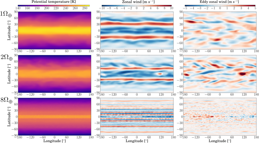
Figure 1.— Potential temperature (left), zonal wind (center), and eddy component of the zonal wind (right) maps at the lowest atmospheric model level for rotation rates of $1,2,~{}\mathrm{and}~{}8~{}\Omega_{\varoplus}$. The surface pressure for these simulations is 1 bar. Eddies that form from baroclinic instabilities are apparent in the mid-latitudes.

To compare with our scaling theory, we perform simulations with the ExoCAM GCM. ExoCAM is a version of the Community Atmosphere Model version 4 with upgraded radiative transfer and water vapor absorption coefficients for application to exoplanets, and has been used for a wide range of exoplanet studies (Kopparapu et al. 2016, 2017; Wolf et al. 2017; Wolf 2017; Haqq-Misra et al. 2018; Komacek & Abbot 2019; Yang et al. 2019). In this work, we use the same basic model setup as Kopparapu et al. (2017); Haqq-Misra et al. (2018); Komacek & Abbot (2019), and Yang et al. (2019): we consider aquaplanets without continents that have immobile slab oceans with a depth of $50~{}\mathrm{m}$ and an atmosphere comprised only of N₂ and H₂O. We consider planets with zero obliquity orbiting a Sun-like star, with varying rotation rates from $0.0625-8\Omega_{\varoplus}$, where $\Omega_{\varoplus}$ is the rotation rate of Earth, and varying surface pressure from $0.25-4~{}\mathrm{bars}$. When varying rotation rate, we keep the surface pressure fixed at 1 bar. Similarly, when we vary surface pressure, we keep the rotation rate fixed to $1\Omega_{\varoplus}$.
These simulations are the same as those in Komacek & Abbot (2019), except that we extend the suite of simulations to faster rotation rates. All simulations assume an incident stellar flux of $1360.8\ \mathrm{W}\ \mathrm{m}^{-2}$, equal to that of Earth. The majority of these simulations use a horizontal resolution of $4^{\circ}\times 5^{\circ}$ with 40 vertical levels and a timestep of $30~{}\mathrm{minutes}$. However, we use a horizontal resolution of $0.47^{\circ}\times 0.63^{\circ}$ and a timestep of $7.5~{}\mathrm{minutes}$ for the fastest rotating case, which has a rotation rate 8 times greater than that of Earth.
Figure 1 shows maps of near-surface potential temperature, zonal wind, and eddy component of the zonal wind from a subset of our GCM simulations with varying rotation rates of $1-8\Omega_{\varoplus}$. The eddy component of the zonal wind is $u^{\prime}=u-\bar{u}$, where $u$ is the zonal wind and $\bar{u}$ is the zonal-mean of the zonal wind. We find that the width of tropical regions decreases and the number of zonal jets increases with increasing rotation rate, as expected from previous work (Rhines 1975; Williams & Holloway 1982; Kaspi & Showman 2015; Wang et al. 2018). We also find that the scale of mid-latitude eddies decreases with increasing rotation rate due to the decreasing deformation radius, as expected from previous work (Schneider & Walker 2006; Kaspi & Schneider 2011, 2013; Wang et al. 2018). This basic understanding qualitatively agrees with that from our scaling theory, which found that the baroclinic criticality parameter should increase with increasing rotation rate.

4. GCM-Theory comparison

4.1. Criticality parameter

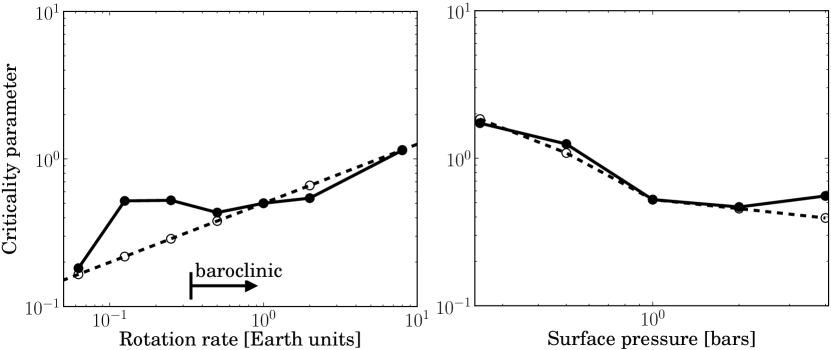
Figure 2.— Scaling for the criticality parameter (dashed lines) compared to GCM results (solid lines) for separately varying rotation rate (left panel) and surface pressure (right panel). For the simulations varying rotation rate (left panel), we keep the surface pressure fixed to 1 bar. For the simulations varying surface pressure (right panel), we keep the rotation rate fixed to that of Earth. We find good agreement between our scaling and GCM results throughout the baroclinically unstable regime, identified by the arrow. However, at rotation rates less than about $1/3\Omega_{\varoplus}$ our scaling under-predicts the criticality parameter, as baroclinic effects weaken.

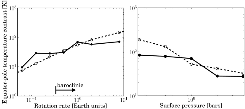
Figure 3.— Scaling for the equator-to-pole temperature contrast (dashed lines) compared to GCM results (solid lines) with varying rotation rate (left panel) and surface pressure (right panel). The equator-to-pole temperature contrast increases with increasing rotation rate and decreasing surface pressure in both our theory and GCM experiments. As a result, we find that our scaling explains the qualitative trends in equator-to-pole temperature contrast throughout the baroclinically unstable regime.

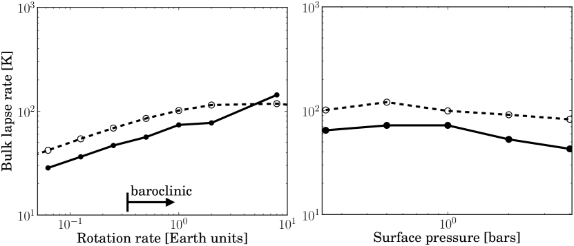
Figure 4.— Scaling for the bulk lapse rate (dashed lines) compared to GCM results for the mid-latitude bulk lapse rate with varying rotation rate (left panel) and surface pressure (right panel). Overall, the variations in bulk lapse rate with planetary parameters are relatively weak compared to the variations in equator-to-pole temperature contrast. As expected from our theory, the bulk lapse rate in our simulations increases with increasing rotation rate up to a maximum at $\approx 8\Omega_{\varoplus}$. The bulk lapse rate increases and then decreases with increasing surface pressure in our simulations, as predicted by our theory.

We calculate the baroclinic criticality parameter from our GCM results similarly to Jansen & Ferrari (2013):

$$\xi=\frac{a\left<\partial\bar{\theta}/\partial y\right>}{H\left<\partial\bar{\theta}/\partial z\right>}\mathrm{,}$$ (15)

where $a=6.37\times 10^{6}~{}\mathrm{m}$ is the planetary radius and $H$ is the smaller of the height of the tropopause and scale height averaged between $30^{\circ}-80^{\circ}$ latitude. The ratio of partial derivatives of potential temperature with respect to latitude and height gives the slope of isentropes from our simulations. We average these partial derivatives from a pressure of $0.5p_{s}$ (where $p_{s}$ is the surface pressure) to the surface and between $30^{\circ}-80^{\circ}$ latitude. Equation (15) calculates the criticality parameter as an average of local isentropic slopes, which is not equivalent to the ratio of the equator-to-pole temperature contrast and bulk lapse rate. We describe the calculation of the equator-to-pole temperature contrast and bulk lapse rate from our GCM experiments in Section 4.2.
Figure 2 shows a comparison of the baroclinic criticality parameter from our GCM results (solid lines) with the scaling theory from Equation (6) (dashed lines) for varying rotation rate and surface pressure. In this comparison, we set $\xi=\xi_{\varoplus}$ for an Earth-like rotation rate and surface pressure. We find that the scaling of criticality parameter as $\Omega^{2/5}$ from Equation (6) is in good agreement with simulations that have rotation rates $\Omega\geq 0.5\Omega_{\varoplus}$ (left panel of Figure 2). The under-prediction of the criticality parameter at slower rotation rates is not surprising, as planets with rotation rates of $\Omega\lesssim 1/3\Omega_{\varoplus}$ have weak baroclinic effects because the deformation radius is larger than the planetary circumference.
We also find good agreement between our theoretical scaling of the criticality parameter with surface pressure and GCM experiments (right hand panel of Figure 2). Note that for the scaling with surface pressure, we include the minimum of the tropopause height and scale height calculated from our GCM experiments in the predicted criticality, because the tropopause height increases with increasing surface pressure. As a result, the decrease of baroclinic criticality with increasing surface pressure is due to the combined effects of increasing surface pressure and increasing tropopause height.

4.2. Equator-to-pole temperature contrast and bulk lapse rate

Figure 3 shows a comparison of the equator-to-pole temperature contrast in the GCM experiments (solid lines) with our theory from Equation (13) (dashed lines) for varying rotation rate and surface pressure. In the GCM results, we average the equator-to-pole temperature contrast from $0.5p_{s}$ to the surface. We keep $\Delta_{h}\theta_{\mathrm{eq}}$ fixed at $242\ \mathrm{K}$, which is the radiative equilibrium emission temperature contrast between the equator and the pole for a zero obliquity planet with Earth’s incident stellar flux. Our estimate of $\Delta_{h}\theta_{\mathrm{eq}}$ assumes an albedo of $0.55$, which is the albedo of our simulation with an Earth-like value of rotation rate and surface pressure. In keeping $\Delta_{h}\theta_{\mathrm{eq}}$ fixed, we ignore changes in the albedo due to changes in the sea ice cover. Notice that, with this choice, there is no tunable parameter in our equations for the equator-to-pole temperature contrast and bulk lapse rate.
We find that the theoretical scalings for the equator-to-pole temperature contrast broadly match those from our GCM experiments, although not as well as for the criticality parameter. The equator-to-pole temperature contrast increases with increasing rotation rate and decreasing surface pressure in our GCM experiments, due to the increased criticality parameter leading to reduced eddy length scales. Note that the equator-to-pole temperature contrast is greatly reduced for simulations with surface pressures of 2 and 4 bars because they are in an ice-covered state due to the lack of CO₂. The change from partial to total ice cover causes a change in $\Delta_{h}\theta_{\mathrm{eq}}$, which is not accounted for in our prediction.
Figure 4 shows the bulk lapse rate calculated from our suite of GCM experiments, averaged between $30-80^{\circ}$ latitude, along with predictions from our theoretical scaling (Equation 14). We find that the bulk lapse rate does not show as strong of a dependence on planetary parameters as the equator-to-pole temperature contrast because our simulations are all near the $\xi\approx 1$ regime. Our theoretical prediction for the bulk lapse rate increases with increasing rotation rate throughout the parameter regime studied, with a maximum at $\approx 8\Omega_{\varoplus}$. This is because $\xi<1$ in our simulations for rotation rates $\Omega<8\Omega_{\varoplus}$ (see Figure 2), and when $\xi<1$ the bulk lapse rate scales with the criticality parameter (see Equation 12). Our prediction for the bulk lapse rate is not strongly dependent on pressure, but does have a maximum at a pressure around $0.5\ \mathrm{bars}$. This maximum at $0.5\ \mathrm{bars}$ occurs because at this surface pressure $\xi\approx 1$, while at lower pressures the criticality parameter $\xi>1$ and at higher pressures $\xi<1$. Our simulations also show a maximum in bulk lapse rate at an intermediate surface pressure, though the maximum occurs at a slightly larger pressure than expected from the theory.

5. Discussion & Conclusions

Our predictions for the equator-to-pole temperature contrast and bulk lapse rate can be tested by future observations of terrestrial exoplanet atmospheres with LUVOIR/HabEx/OST. We predict that the equator-to-pole temperature contrast should increase with increasing rotation rate and decreasing surface pressure. Our theoretical predictions can be tested by observationally constraining the equator-to-pole temperature contrast. It may be possible to constrain the equator-to-pole temperature contrast for planets with non-zero obliquity, as both their polar and equatorial regions are visible throughout one planetary rotation (Cowan & Fujii 2018; Olson et al. 2018). Our scalings show that, when varying only rotation rate and considering fixed incident stellar flux, surface pressure, and atmospheric composition, planets with faster rotation rates will have colder poles. As a result, planets in a cold climate regime like those simulated in this work should have wider ice coverage with increasing rotation rate, which could be detectable through albedo variations over planetary orbital phase.
We predict that the bulk lapse rate is only weakly dependent on planetary parameters relative to the equator-to-pole temperature contrast. We also found that the bulk lapse rate has a maximum for planets with baroclinic criticality parameters $\xi\approx 1$. For Earth-like planets with rotation rates $\Omega\lesssim 8\Omega_{\varoplus}$, we find in our GCM experiments that the bulk lapse rate increases with rotation rate, while for faster rotating planets the bulk lapse rate should decrease with increasing rotation rate. We also find that the bulk lapse rate is very weakly dependent on surface pressure, with less than a factor of two variation when increasing the surface pressure from 0.25 to 4 bars. The bulk lapse rate is related to the vertical potential temperature contrast. Planets with greater vertical potential temperature contrasts have more stably stratified atmospheres with smaller in-situ temperature lapse rates. As a result, a large bulk (potential temperature) lapse rate implies a small in-situ temperature lapse rate. In this way, our predictions for the bulk lapse rate can be tested with inverse (retrieval) methods that constrain the atmospheric lapse rate from an observed spectrum, which have been applied widely to interpret previous exoplanet observations (Madhusudhan & Seager 2009; Benneke & Seager 2012; Line & Yung 2013; Waldmann et al. 2015; Feng et al. 2016). Retrieval methods can determine the height of the top of the tropospheric cloud layer (Feng et al. 2018), which occurs approximately at the tropopause. Given the height of the tropopause, we can relate the bulk lapse rate directly to the temperature lapse rate and compare it to our theoretical prediction.
We tested our analytic theory using simulations of terrestrial exoplanets with varying rotation rate and surface pressure. However, this suite of simulations was limited in extent, as we kept the atmospheric composition and host stellar spectrum fixed. We only considered an N₂-H₂O atmosphere without additional greenhouse gases, and as a result our simulations are in a relatively cold climate regime with large sea-ice coverage, relatively little water vapor, and weak latent heat transport. If our simulations were instead in a warm climate regime, for example by including an Earth-like complement of greenhouse gases, the equator to pole temperature contrast would be smaller (Kaspi & Showman 2015; Jansen et al. 2019). Additionally, we used the Solar incident spectrum for our suite of simulations. Near-IR absorption by water vapor could change the bulk lapse rate from that predicted by our theory for non-tidally locked planets that orbit later spectral type host stars than the Sun (Cronin & Jansen 2016).
Our theoretical model, while applicable throughout a wide range of parameter space, can only be applied to predict the atmospheric circulation of planets that have baroclinically unstable atmospheres. Baroclinic effects are significantly weaker on slowly rotating planets that have deformation radii which are larger than the planetary circumference. As a result, our theory does not apply to Earth-sized planets with rotation periods $\gtrsim 3~{}\mathrm{days}$. Note that Earth-like planets could have a wide range of spin rates, with rotation periods ranging from $1-10^{4}\ \mathrm{hr}$ due to the stochastic nature of the oligarchic stage of planetary growth (Miguel & Brunini 2010). Additionally, Earth itself rotated faster in the past, as its rotation is slowed due to tidal interactions with the Moon. The theory presented here cannot be applied to slowly-rotating terrestrial planets orbiting Sun-like stars or tidally locked planets orbiting M dwarf stars. However, Wordsworth (2015) and Koll & Abbot (2016) have developed theories for the temperature structure and wind speeds of tidally locked terrestrial planets. Additionally, theories developed to understand circulation in the tropical regions of Earth (Held & Hou 1980; Held 2000; Sobel et al. 2001; Chemke & Kaspi 2017) can be used to understand the atmospheric heat transport of slowly rotating planets orbiting Sun-like stars.
Our scaling theory could also help with the interpretation of observations of warm Jupiter and warm Neptune exoplanets with the James Webb Space Telescope (JWST). Baroclinic instabilities play a key role in driving the zonal jets in Jupiter’s atmosphere (Williams 1978; Gierasch et al. 1979; Williams 1979; Kaspi & Flierl 2006; Lian & Showman 2008; Young et al. 2019), and likely affect the circulation of fast-rotating gas giant exoplanets. Previous work has studied how the atmospheric circulation of warm Jupiters depends on rotation rate, incident stellar flux, and obliquity (Showman et al. 2015; Rauscher 2017). Showman et al. (2015) found that the equator-to-pole temperature contrast of warm Jupiters increases with increasing rotation rate, as expected from our scaling theory. Emission spectra with JWST will constrain the temperature-pressure profiles of warm Jupiters and warm Neptunes (Greene et al. 2016), which may also be affected by baroclinic instabilities.
In this work, we extended Earth-based theoretical scalings for baroclinic instability to estimate basic quantities of the circulation of terrestrial exoplanets. Our scalings can be used to predict the baroclinic criticality parameter throughout the baroclinically unstable regime of terrestrial exoplanets. As the criticality parameter is directly linked to the slope of isentropes, we apply these scalings to estimate the equator-to-pole temperature contrast and bulk lapse rate. These scalings predict that the equator-to-pole temperature contrast increases with increasing rotation rate and decreasing surface pressure, while the bulk lapse rate depends relatively weakly on variations in planetary parameters around Earth-like values and has a maximum when the criticality parameter is near one. We find reasonable agreement between the equator-to-pole temperature contrast and bulk lapse rate predicted by our scaling theory and simulated using a detailed GCM. This agreement extends throughout the parameter regime of Earth-sized exoplanets with rotation rates $\gtrsim 1/3\Omega_{\varoplus}$, but for more slowly rotating planets baroclinic effects are small and our theory no longer applies.

References

- Baker et al. (2019) Baker, A., Blake, C., & Halverson, S. 2019, Publications of the Astronomical Society of the Pacific, 131, 064402
- Benneke & Seager (2012) Benneke, B. & Seager, S. 2012, The Astrophysical Journal, 753, 100
- Chai & Vallis (2014) Chai, J. & Vallis, G. 2014, Journal of the Atmospheric Sciences, 71, 2300
- Charney (1947) Charney, J. 1947, Journal of Meteorology, 4, 135
- Chemke & Kaspi (2017) Chemke, R. & Kaspi, Y. 2017, The Astrophysical Journal, 841, 1
- Cowan & Fujii (2018) Cowan, N. & Fujii, Y. Handbook of Exoplanets, ed. H. Deeg & J. Belmonte (Springer)
- Cowan et al. (2009) Cowan, N. B., Agol, E., Meadows, V. S., Robinson, T., Livengood, T. A., Deming, D., Lisse, C. M., A’Hearn, M. F., Wellnitz, D. D., Seager, S., & Charbonneau, D. 2009, The Astrophysical Journal, 700, 915
- Cowan & Strait (2013) Cowan, N. B. & Strait, T. E. 2013, The Astrophysical Journal Letters, 765, L17
- Cronin & Jansen (2016) Cronin, T. & Jansen, M. 2016, Geophysical Research Letters, 43, 449
- Eady (1949) Eady, E. 1949, Tellus, 1, 33
- Feng et al. (2016) Feng, Y., Line, M., Fortney, J., Stevenson, K., Bean, J., Kreidberg, L., & Parmentier, V. 2016, The Astrophysical Journal, 829, 52
- Feng et al. (2018) Feng, Y., Robinson, T., Fortney, J., Lupu, R., Marley, M., Lewis, N., Macintosh, B., & Line, M. 2018, The Astronomical Journal, 155, 200
- Gierasch et al. (1979) Gierasch, P., Ingersoll, A., & Pollard, D. 1979, Icarus, 40, 205
- Greene et al. (2016) Greene, T., Line, M., Montero, C., Fortney, J., Lustig-Yaeger, J., & Luther, K. 2016, The Astrophysical Journal, 817, 17
- Haqq-Misra et al. (2018) Haqq-Misra, J., Wolf, E., Josh, M., Zhang, X., & Kopparapu, R. 2018, The Astrophysical Journal, 852, 67
- Held (2000) Held, I. 2000, in Program in Geophysical Fluid Dynamics (Woods Hole, MA: Woods Hole Oceanographic Institute)
- Held (2007) —. The Global Circulation of the Atmosphere, ed. T. Schneider & A. Sobel (Princeton University Press), 1
- Held & Hou (1980) Held, I. & Hou, A. 1980, Journal of the Atmospheric Sciences, 37, 515
- Held & Larichev (1996) Held, I. & Larichev, V. 1996, Journal of the Atmospheric Sciences, 53, 946
- Jansen & Ferrari (2012a) Jansen, M. & Ferrari, R. 2012a, Journal of the Atmospheric Sciences, 69, 695
- Jansen & Ferrari (2012b) —. 2012b, Journal of the Atmospheric Sciences, 70, 1456
- Jansen & Ferrari (2013) —. 2013, Journal of the Atmospheric Sciences, 70, 2948
- Jansen et al. (2019) Jansen, T., Scharf, C., Way, M., & Genio, A. D. 2019, The Astrophysical Journal, 875, 79
- Kang (2019a) Kang, W. 2019a, The Astrophysical Journal Letters, 876, L1
- Kang (2019b) —. 2019b, The Astrophysical Journal Letters, 877, L6
- Kaspi & Flierl (2006) Kaspi, Y. & Flierl, G. 2006, Journal of the Atmospheric Sciences, 64, 3177
- Kaspi & Schneider (2011) Kaspi, Y. & Schneider, T. 2011, Journal of the Atmospheric Sciences, 68, 2459
- Kaspi & Schneider (2013) —. 2013, Journal of the Atmospheric Sciences, 70, 2596
- Kaspi & Showman (2015) Kaspi, Y. & Showman, A. 2015, The Astrophysical Journal, 804, 60
- Kawahara & Fujii (2010) Kawahara, H. & Fujii, Y. 2010, The Astrophysical Journal, 720, 1333
- Koll & Abbot (2016) Koll, D. & Abbot, D. 2016, The Astrophysical Journal, 825, 99
- Komacek & Abbot (2019) Komacek, T. & Abbot, D. 2019, The Astrophysical Journal, 871, 245
- Kopparapu et al. (2017) Kopparapu, R., Wolf, E., Arney, G., Batalha, N., Haqq-Misra, J., Grimm, S., & Heng, K. 2017, The Astrophysical Journal, 845, 5
- Kopparapu et al. (2016) Kopparapu, R., Wolf, E., Haqq-Misra, J., Yang, J., Kasting, J., Meadows, V., Terrien, R., & Mahadevan, S. 2016, The Astrophysical Journal, 819, 84
- Kreidberg & Loeb (2016) Kreidberg, L. & Loeb, A. 2016, The Astrophysical Journal Letters, 832, L12
- Lian & Showman (2008) Lian, Y. & Showman, A. 2008, Icarus, 194, 597
- Line & Yung (2013) Line, M. & Yung, Y. 2013, The Astrophysical Journal, 779, 3
- Lustig-Yaeger et al. (2018) Lustig-Yaeger, J., Meadows, V., Mendoza, G., Schwieterman, E., Fujii, Y., Luger, R., & Robinson, T. 2018, The Astronomical Journal, 156, 301
- Madhusudhan & Seager (2009) Madhusudhan, N. & Seager, S. 2009, The Astrophysical Journal, 707, 24
- Miguel & Brunini (2010) Miguel, Y. & Brunini, A. 2010, Monthly Notices of the Royal Astronomical Society, 406, 1935
- Molliere & Snellen (2019) Molliere, P. & Snellen, I. 2019, Astronomy & Astrophysics, 622, A139
- Morley et al. (2017) Morley, C., Kreidberg, L., Rustamkulov, Z., Robinson, T., & Fortney, J. 2017, The Astrophysical Journal, 850, 121
- Olson et al. (2018) Olson, S., Schwieterman, E., Reinhard, C., Ridgewell, A., Kane, S., Meadows, V., & Lyons, T. 2018, The Astrophysical Journal Letters, 858, L14
- Pierrehumbert (2010) Pierrehumbert, R. 2010, Principles of Planetary Climate (Cambridge: Cambridge University Press)
- Popp et al. (2016) Popp, M., Schmidt, H., & Marotzke, J. 2016, Nature Communications, 7, 10627
- Rauscher (2017) Rauscher, E. 2017, The Astrophysical Journal, 846, 69
- Rhines (1975) Rhines, P. 1975, Journal of Fluid Mechanics, 69, 417
- Schneider (2004) Schneider, T. 2004, Journal of the Atmospheric Sciences, 61, 1317
- Schneider & Walker (2006) Schneider, T. & Walker, C. 2006, Journal of the Atmospheric Sciences, 63, 1569
- Showman & Guillot (2002) Showman, A. & Guillot, T. 2002, Astronomy and Astrophysics, 385, 166
- Showman et al. (2015) Showman, A., Lewis, N., & Fortney, J. 2015, The Astrophysical Journal, 801, 95
- Showman et al. (2013) Showman, A., Wordsworth, R., Merlis, T., & Kaspi, Y. Comparative Climatology of Terrestrial Planets, ed. S. Mackwell, A. Simon-Miller, J. Harder, & M. Bullock (Tucson, AZ: University of Arizona Press)
- Snellen et al. (2015) Snellen, I., de Kok, R., Birkby, J., Brandl, B., Brogi, M., Keller, C., Kenworthy, M., Schwarz, H., & Stuik, R. 2015, Astronomy & Astrophysics, 576, A59
- Sobel et al. (2001) Sobel, A., Nilsson, J., & Polvani, L. 2001, Journal of the Atmospheric Sciences, 58, 3650
- Stone (1978) Stone, P. 1978, Journal of the Atmospheric Sciences, 35, 561
- Vallis (2006) Vallis, G. 2006, Atmospheric and Oceanic Fluid Dynamics: Fundamentals and Large-Scale Circulation (Cambridge: Cambridge University Press)
- Waldmann et al. (2015) Waldmann, I., Tinetti, G., Rocchetto, M., Barton, E., Yurchenko, S., & Tennyson, J. 2015, The Astrophysical Journal, 802, 107
- Wang et al. (2018) Wang, Y., Read, P., Tabataba-Vakili, F., & Young, R. 2018, Quarterly Journal of the Royal Meteorological Society, 144, 2537
- Way et al. (2017) Way, M., Aleinov, I., Amundsen, D., Chandler, M., Clune, T., Genio, A. D., Fujii, Y., Kelley, M., Kiang, N., Sohl, L., & Tsigaridis, K. 2017, The Astrophysical Journal Supplement Series, 231, 12
- Williams (1978) Williams, G. 1978, Journal of the Atmospheric Sciences, 35, 1399
- Williams (1979) —. 1979, Journal of the Atmospheric Sciences, 36, 932
- Williams & Holloway (1982) Williams, G. & Holloway, J. 1982, Nature, 297, 295
- Wolf (2017) Wolf, E. 2017, The Astrophysical Journal Letters, 839, L1
- Wolf et al. (2017) Wolf, E., Shields, A., Kopparapu, R., Haqq-Misra, J., & Toon, O. 2017, The Astrophysical Journal, 837, 107
- Wordsworth (2015) Wordsworth, R. 2015, The Astrophysical Journal, 806, 180
- Yang et al. (2019) Yang, H., Komacek, T., & Abbot, D. 2019, The Astrophysical Journal Letters, 876, L27
- Yang et al. (2014) Yang, J., Boue, G., Fabrycky, D., & Abbot, D. 2014, The Astrophysical Journal Letters, 787, L2
- Young et al. (2019) Young, R., Read, P., & Wang, Y. 2019, Icarus, 326, 225