Audio-visual Speech Enhancement Using Conditional Variational Auto-Encoders

Abstract

Variational auto-encoders (VAEs) are deep generative latent variable models that can be used for learning the distribution of complex data. VAEs have been successfully used to learn a probabilistic prior over speech signals, which is then used to perform speech enhancement. One advantage of this generative approach is that it does not require pairs of clean and noisy speech signals at training. In this paper, we propose audio-visual variants of VAEs for single-channel and speaker-independent speech enhancement. We develop a conditional VAE (CVAE) where the audio speech generative process is conditioned on visual information of the lip region. At test time, the audio-visual speech generative model is combined with a noise model based on nonnegative matrix factorization, and speech enhancement relies on a Monte Carlo expectation-maximization algorithm. Experiments are conducted with the recently published NTCD-TIMIT dataset as well as the GRID corpus. The results confirm that the proposed audio-visual CVAE effectively fuses audio and visual information, and it improves the speech enhancement performance compared with the audio-only VAE model, especially when the speech signal is highly corrupted by noise. We also show that the proposed unsupervised audio-visual speech enhancement approach outperforms a state-of-the-art supervised deep learning method.

I Introduction

The problem of speech enhancement (SE) consists in estimating clean-speech signals from noisy single-channel or multiple-channel audio recordings. There is a long tradition of audio speech enhancement (ASE) methods and associated algorithms, software and systems, e.g. [1, 2, 3]. In this paper we address the problem of audio-visual speech enhancement (AVSE): in addition to audio, we exploit the benefits of visual speech information available with video recordings of lip movements. The rationale of AVSE is that, unlike audio information, visual information (lip movements) is not corrupted by acoustic perturbations, and hence visual information can help the speech enhancement process, in particular in the presence of audio signals with low signal-to-noise ratios.

Although it has been shown that the fusion of visual and audio information is beneficial for various speech perception tasks, e.g. [4, 5, 6], AVSE has been far less investigated than ASE. AVSE methods can be traced back to [7] and subsequent work, e.g. [8, 9, 10, 11, 12, 13]. Not surprisingly, AVSE has been recently addressed in the framework of deep neural networks and a number of interesting architectures and well-performing algorithms were developed, e.g. [14, 15, 16, 17, 18].

In this paper we propose to fuse single-channel audio and single-camera visual information for speech enhancement in the framework of variational auto-encoders. This may well be viewed as a multimodal extension of VAE-based methods of [19, 20, 21, 22, 23, 24] which, up to our knowledge, yield state-of-the-art ASE performance in an unsupervised learning setting. In order to incorporate visual observations into the VAE speech enhancement framework, we propose to use conditional variational auto-encoders [25]. As in [20] we proceed in three steps.

First, the parameters of the audio-visual CVAE (AV-CVAE) architecture are learned using synchronized clean audio-speech and visual-speech data. This yields an audio-visual speech prior model. The training is totally unsupervised, in the sense that speech signals mixed with various types of noise signal are not required. This stays in contrast with supervised DNN methods that need to be trained in the presence of many noise types and noise levels in order to ensure generalization and good performance, e.g. [14, 15, 16, 26]. Second, the learned speech prior is used in conjunction with a mixture model and with a nonnegative matrix factorization (NMF) noise variance model, to infer both the gain, which models the time-varying loudness of the speech signal, and the NMF parameters. Third, the clean speech is reconstructed using the speech prior (VAE parameters) as well as the inferred gain and noise variance. The latter may well be viewed as a probabilistic Wiener filter. The learned VAE architecture and its variants, the gain- and noise- parameter inference algorithms, and the proposed speech reconstruction method are thoroughly tested and compared with a state-of-the-art method, using the NTCD-TIMIT dataset [27] as well as the GRID corpus [28] containing audio-visual recordings.

The remainder of the paper is organized as follows. Section II summarizes related work. In Section III we briefly review how to use a VAE to model the speech prior distribution. Then, in Section IV we introduce two VAE network variants for learning the speech prior from visual data. In Section V, we present the proposed AV-CVAE used to model the acoustic speech distribution conditioned by visual information. In Section VI, we discuss the inference phase, i.e., the actual speech enhancement process. Finally, our experimental results are presented in Section VII.

II Related Work

Speech enhancement has been an extremely investigated topic for the last decades and a complete state of the art is beyond the scope of this paper. We briefly review the literature on single-channel SE and then we discuss the most significant work in AVSE.

Classical methods use spectral subtraction [29] and Wiener filtering [30] based on noise and/or speech power spectral density (PSD) estimation in the short-time Fourier transform (STFT) domain. Another popular family of methods is the short-term spectral amplitude estimator [31], initially based on a local complex-valued Gaussian model of the speech STFT coefficients and then extended to other density models [32, 33], and to a log-spectral amplitude estimator [34, 35]. A popular technique for modeling the PSD of speech signals [36] is NMF, e.g., [37, 38, 39].

More recently, SE has been addressed in the framework of DNNs [40]. Supervised methods learn mappings between noisy-speech and clean-speech spectrograms, which are then used to reconstruct a speech waveform [41, 42, 43]. Alternatively, the noisy input is mapped onto a time frequency (TF) mask, which is then applied to the input to remove noise and to preserve speech information as much as possible [44, 45, 46, 26]. In order for these supervised learning methods to generalize well and to yield state-of-the-art results, the training data must contain a large variability in terms of speakers and, even more critically, in terms of noise types and noise levels [44, 42]; in practice this leads to cumbersome learning processes. Alternatively, generative (or unsupervised) DNNs do not use any kind of noise information for training, and for this reason they are very interesting because they have very good generalization capabilities. An interesting generative formulation is provided by VAEs [47]. Combined with NMF, VAE-based methods yield state-of-the-art SE performance [19, 20, 21, 22, 23, 24] for an unsupervised learning setting. VAEs conditioned on the speaker identity have also been used for speaker-dependent multi-microphone speech separation [48, 49] and dereverberation [50].

The use of visual cues to complement audio, whenever the latter is noisy, ambiguous or incomplete, has been thoroughly studied in psychophysics [4, 5, 6]. Indeed, speech production implies simultaneous air circulation through the vocal tract and tongue and lip movements, and hence speech perception is multimodal. Several computational models were proposed to exploit the correlation between audio and visual information for the perception of speech, e.g. [9, 12]. A multi-layer perceptron architecture was proposed in [8] to map noisy-speech linear prediction features concatenated with visual features onto clean-speech linear prediction features. Then Wiener filters were built for denoising. Audio-visual Wiener filtering was later extended using phoneme-specific Gaussian mixture regression and filterbank audio features [51] . Other AVSE methods exploit noise-free visual information [10, 11] or make use of twin hidden Markov models (HMMs) [13].

State-of-the-art supervised AVSE methods are based on DNNs. The rationale of [14, 16] is to use visual information to predict a TF soft mask in the STFT domain and to apply this mask to the audio input in order to remove noise. In [16] a video-to-speech architecture is trained for each speaker in the dataset, which yields a speaker-dependent AVSE method. The architecture of [14] is composed of a magnitude subnetwork that takes both visual and audio data as inputs, and a phase subnetwork that only takes audio as input. Both subnetworks are trained using ground-truth clean speech. Then, the magnitude subnetwork predicts a binary mask which is then applied to both the magnitude and phase spectrograms of the input signal, thus predicting a filtered speech spectrogram. The architectures of [17] and [15] are quite similar: they are composed of two subnetworks, one for processing noisy speech and one for processing visual speech. The two encodings are then concatenated and processed to eventually obtain an enhanced speech spectrogram. The main difference between [17] and [15] is that the former predicts both enhanced visual and audio speech, while the latter predicts only audio speech. The idea of obtaining a binary mask for separating speech of an unseen speaker from an unknown noise was exploited in [18]: a hybrid DNN model integrates a stacked long short-term memory (LSTM) and convolutional LSTM for audio-visual (AV) mask estimation.

In the supervised deep learning methods just mentioned, generalization to unseen data is a critical issue. The major issues are noise and speaker variability. Therefore, training these methods requires noisy mixtures with a large number of noise types and speakers, in order to guarantee generalization. In comparison, the proposed method is totally unsupervised: its training is based on VAEs and it only requires clean audio speech and visual speech. The gain and the noise variance are estimated at testing using a Monte Carlo expectation-maximization (MCEM) algorithm [52]. The clean speech is then reconstructed from the audio and visual inputs using the learned parameters. The latter may well be viewed as a probabilistic Wiener filter. This stays in contrast with the vast majority of supervised DNN-based AVSE methods that predict a TF mask which is applied to the noisy input. Empirical validation, based on standard SE scores and using a widely used publicly available dataset, shows that our method outperforms the ASE method [20] as well as the state-of-the-art supervised AVSE method [15].

III Audio VAE

In this section, we briefly review the deep generative speech model that was first proposed in [19] along with its parameters estimation procedure using VAEs [47]. Let $s_{fn}$ denote the complex-valued speech STFT coefficient at frequency index $f\in\{0,...,F-1\}$ and at frame index $n$. At each TF bin, we have the following model which will be referred to as audio VAE (A-VAE):

$$s_{fn}|\mathbf{z}_{n} \sim\mathcal{N}_{c}(0,\sigma_{f}(\mathbf{z}_{n})),$$ (1)

$$\mathbf{z}_{n} \sim\mathcal{N}(\mathbf{0},\mathbf{I})$$ (2)

where $\mathbf{z}_{n}\in\mathbb{R}^{L}$, with $L\ll F$, is a latent random variable describing a speech generative process, $\mathcal{N}(\mathbf{0},\mathbf{I})$ is a zero-mean multivariate Gaussian distribution with identity covariance matrix, and $\mathcal{N}_{c}(0,\sigma)$ is a univariate complex proper Gaussian distribution with zero mean and variance $\sigma$. Let $\mathbf{s}_{n}\in\mathbb{C}^{F}$ be the vector whose components are the speech STFT coefficients at frame $n$. The set of non-linear functions $\{\sigma_{f}:\mathbb{R}^{L}\mapsto\mathbb{R}_{+}\}_{f=0}^{F-1}$ are modeled as neural networks sharing the input $\mathbf{z}_{n}\in\mathbb{R}^{L}$. The parameters of these neural networks are collectively denoted with $\boldsymbol{\theta}$. This variance can be interpreted as a model for the short-term PSD of the speech signal.

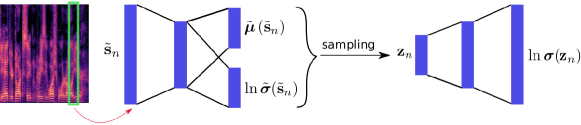
Figure 1: The A-VAE network used for learning a speech prior using audio data. The encoder network (left) takes as input the squared magnitude vector $\tilde{{\bf s}}_{n}$, associated with the STFT frame ${\bf s}_{n}$ (outlined in green), and outputs the mean and variance of the posterior distribution $q\left(\mathbf{z}_{n}|{{\bf s}}_{n};\boldsymbol{\psi}\right)$. The decoder network (right) takes ${\bf z}_{n}$ as input (sampled from the posterior distribution) and outputs the variance of $p({\bf s}_{n}|{\bf z}_{n};\boldsymbol{\theta})$.

An important property of VAEs is to provide an efficient way of learning the parameters $\boldsymbol{\theta}$ of such generative models [47], taking ideas from variational inference [53, 54]. Let $\mathbf{s}=\{\mathbf{s}_{n}\in\mathbb{C}^{F}\}_{n=0}^{N_{tr}-1}$ be a training dataset of clean-speech STFT frames and let $\mathbf{z}=\{\mathbf{z}_{n}\in\mathbb{R}^{L}\}_{n=0}^{N_{tr}-1}$ be the associated latent variables. In the VAE framework, the parameters $\boldsymbol{\theta}$ are estimated by maximizing a lower bound of the log-likelihood, $\ln p(\mathbf{s};\boldsymbol{\theta})$, called evidence lower bound (ELBO), defined by:

$$\mathcal{L}\left({\bf s};\boldsymbol{\theta},\boldsymbol{\psi}\right)=\mathbb{E}_{q\left(\mathbf{z}|\mathbf{s};\boldsymbol{\psi}\right)}\left[\ln p\left(\mathbf{s}|\mathbf{z};\boldsymbol{\theta}\right)\right]-D_{\text{KL}}\left(q\left(\mathbf{z}|\mathbf{s};\boldsymbol{\psi}\right)\parallel p(\mathbf{z})\right),$$ (3)

where $q\left(\mathbf{z}|\mathbf{s};\boldsymbol{\psi}\right)$ denotes an approximation of the intractable true posterior distribution $p(\mathbf{z}|\mathbf{s};\boldsymbol{\theta})$, $p(\mathbf{z})$ is the prior distribution of ${\bf z}$, and $D_{\text{KL}}(q\parallel p)=\mathbb{E}_{q}[\ln(q/p)]$ is the Kullback-Leibler divergence. Independently, for all $l\in\{0,...,L-1\}$ and all $n\in\{0,...,N_{tr}-1\}$, $q(\mathbf{z}|\mathbf{s};\boldsymbol{\psi})$ is defined by:

$$z_{ln}|\mathbf{s}_{n}\sim\mathcal{N}\left(\tilde{\mu}_{l}\left(\tilde{\mathbf{s}}_{n}\right),\tilde{\sigma}_{l}\left(\tilde{\mathbf{s}}_{n}\right)\right),$$ (4)

where $\tilde{\mathbf{s}}_{n}\triangleq(|s_{0n}|^{2}\dots|s_{F-1\>n}|^{2})^{\top}$. The non-linear functions $\{\tilde{\mu}_{l}:\mathbb{R}_{+}^{F}\mapsto\mathbb{R}\}_{l=0}^{L-1}$ and $\{\tilde{\sigma}_{l}:\mathbb{R}_{+}^{F}\mapsto\mathbb{R}_{+}\}_{l=0}^{L-1}$ are modeled as neural networks, sharing as input the speech power spectrum frame $\tilde{\mathbf{s}}_{n}$, and collectively parameterized by $\boldsymbol{\psi}$. The parameter set $\boldsymbol{\psi}$ is also estimated by maximizing the variational lower bound defined in (3), which is actually equivalent to minimizing the Kullback-Leibler divergence between $q\left(\mathbf{z}|\mathbf{s};\boldsymbol{\psi}\right)$ and the intractable true posterior distribution $p(\mathbf{z}|\mathbf{s};\boldsymbol{\theta})$ [53]. Using (1), (2) and (4) we can develop this objective function as follows:

$$\mathcal{L}\left({\bf s};\boldsymbol{\theta},\boldsymbol{\psi}\right)\overset{c}{=} -\sum_{f=0}^{F-1}\sum_{n=0}^{N_{tr}-1}\mathbb{E}_{q\left(\mathbf{z}_{n}|\mathbf{s}_{n};\boldsymbol{\psi}\right)}\left[d_{\text{IS}}\left(\left|s_{fn}\right|^{2};\sigma_{f}(\mathbf{z}_{n})\right)\right]$$

$$+\frac{1}{2}\sum_{l=0}^{L-1}\sum_{n=0}^{N_{tr}-1}\left[\ln\tilde{\sigma}_{l}\left(\tilde{\mathbf{s}}_{n}\right)-\tilde{\mu}^{2}_{l}\left(\tilde{\mathbf{s}}_{n}\right)-\tilde{\sigma}_{l}\left(\tilde{\mathbf{s}}_{n}\right)\right],$$ (5)

where $d_{\text{IS}}(x;y)=x/y-\ln(x/y)-1$ is the Itakura-Saito divergence [36]. Finally, using sampling techniques combined with the so-called “reparametrization trick” [47] to approximate the intractable expectation in (5), one obtains an objective function which is differentiable with respect to both $\boldsymbol{\theta}$ and $\boldsymbol{\psi}$ and can be optimized using gradient-ascent algorithms [47]. The encoder-decoder architecture of the A-VAE speech prior is summarized in Figure 1.

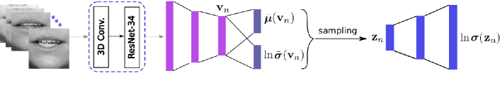
Figure 2: The two V-VAE network variants (base and augmented) for learning speech prior from visual features. A lip ROI is embedded into a visual feature vector, denoted $\mathbf{v}_{n}$, which is encoded and decoded using the same architecture and the same learning method as A-VAE. Optionally, one can also use a pre-trained network (dashed box) composed of a 3D convolution layer followed by a ResNet with 34 layers.

IV Visual VAE

We now introduce two VAE network variants for learning the speech prior from visual data, that will be referred to as base visual VAE (V-VAE) and augmented V-VAE, and which are summarized in Figure 2. As it can be seen, this architecture is similar to A-VAE, with the notable difference that it takes as input visual observations, namely lip images. In more detail, standard computer vision algorithms are used to extract a fixed-sized bounding-box from the image of a speaking face, with the lips in its center, i.e. a lip ROI. This ROI is embedded into a visual feature vector $\mathbf{v}_{n}\in\mathbb{R}^{M}$ using a two-layer fully-connected network, referred below as the base network, where $M$ is the dimension of the visual embedding. Optionally, one can use an additional pre-trained front-end network (dashed box) composed of a 3D convolution layer followed by a ResNet with 34 layers, as part of a network specifically trained for the task of supervised audio-visual speech recognition [55]. This second option is referred to as augmented V-VAE.

In variational inference [53, 54], any distribution over the latent variables $\mathbf{z}$ can be considered for approximating the intractable posterior $p(\mathbf{z}|\mathbf{s};\boldsymbol{\theta})$ and for defining the ELBO. For the V-VAE model, we explore the use of an approximate posterior distribution $q({\bf z}|{\mathbf{v}};\boldsymbol{\gamma})$ defined by:

$$z_{ln}|{\mathbf{v}}_{n}\sim\mathcal{N}\left(\bar{\mu}_{l}({\mathbf{v}}_{n}),\bar{\sigma}_{l}({\mathbf{v}}_{n})\right),$$ (6)

where $\mathbf{v}=\{\mathbf{v}_{n}\}_{n=1}^{N_{tr}-1}$ is the training set of visual features, and where the non-linear functions $\{\bar{\mu}_{l}:{\mathbb{R}}^{M}\mapsto\mathbb{R}\}_{l=0}^{L-1}$ and $\{\bar{\sigma}_{l}:{\mathbb{R}}^{M}\mapsto\mathbb{R}_{+}\}_{l=0}^{L-1}$ are collectively modeled with a neural network parameterized by $\gamma$ and which takes ${\mathbf{v}}_{n}$ as input. Notice that V-VAE and A-VAE share the same decoder architecture, i.e. (1). Eventually, the objective function of V-VAE has the same structure as (5) and hence one can use the same gradient-ascent algorithm as above to estimate the parameters of the V-VAE network.

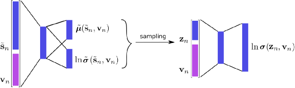
Figure 3: Pipeline of the proposed AV-CVAE architecture for learning an audio-visual speech prior for speech enhancement. The encoder takes a single frame of squared magnitude of speech’s STFT, denoted by $\tilde{{\bf s}}_{n}$, as well as the corresponding visual feature vector ${\mathbf{v}}_{n}$, and outputs the parameters of the posterior distribution $q\left(\mathbf{z}_{n}|{{\bf s}}_{n},{\mathbf{v}}_{n};\boldsymbol{\psi}\right)$. The decoder network takes ${\bf z}_{n}$, sampled from the posterior distribution, together with ${\mathbf{v}}_{n}$ as input and outputs the variance of $p({{\bf s}}_{n}|{\bf z}_{n},{\mathbf{v}}_{n};\boldsymbol{\theta})$.

V Audio-visual VAE

We now investigate an audio-visual VAE model, namely a model that combines audio speech with visual speech. The rationale behind this multimodal approach is that audio data are often corrupted by noise while visual data are not. Without loss of generality, it will be assumed that audio and visual data are synchronized, i.e. there is a video frame associated with each audio frame.

In order to combine the above A-VAE and V-VAE formulations, we consider the CVAE framework to learn structured-output representations [25]. At training, a CVAE is provided with data as well as with associated class labels, such that the network is able to learn a structured data distribution. At test, the trained network is provided with a class label to generate samples from the corresponding class. CVAEs have been proven to be very effective for missing-value inference problems, e.g., computer vision problems with partially available input-output pairs [25].

In the case of AV speech enhancement we consider a training set of $N_{tr}$ synchronized frames of AV features, namely $(\mathbf{s},\mathbf{v})=\{\mathbf{s}_{n},\mathbf{v}_{n}\}_{n=1}^{N_{tr}-1}$ where, as above, ${\mathbf{v}}_{n}\in\mathbb{R}^{M}$ is a lip ROI embedding. The clean audio speech, which is only available at training, is conditioned on the observed visual speech. The visual information is however available both at training and at testing, therefore it serves as a deterministic prior on the desired clean audio speech. Interestingly, it also affects the prior distribution of ${\bf z}_{n}$. To summarize, the following latent space model is considered, independently for all $l\in\{0,...,L-1\}$ and all TF bins $(f,n)$:

$$s_{fn}|\mathbf{z}_{n},{\mathbf{v}}_{n} \sim\mathcal{N}_{c}(0,\sigma_{f}(\mathbf{z}_{n},{\mathbf{v}}_{n})),$$ (7)

$$z_{ln}|{\mathbf{v}}_{n} \sim\mathcal{N}\left(\bar{\mu}_{l}({\mathbf{v}}_{n}),\bar{\sigma}_{l}({\mathbf{v}}_{n})\right),$$ (8)

where the non-linear functions $\{{\sigma}_{f}:{\mathbb{R}}^{L}\times{\mathbb{R}}^{M}\mapsto\mathbb{R}_{+}\}_{f=0}^{F-1}$ are modeled as a neural network parameterized by $\boldsymbol{\theta}$ and taking ${\bf z}_{n}$ and ${\mathbf{v}}_{n}$ as input, and where (8) is identical with (6) but the corresponding parameter set $\gamma$ will have different estimates, as explained below. Also, notice that $\sigma_{f}$ in (1) and in (7) are different, but they both correspond to the PSD of the generative speech model. This motivates the abuse of notation that holds through the paper. The proposed architecture is referred to as AV-CVAE and is shown in Fig. 3. Compared to A-VAE of Section III and Figure 1 and with V-VAE of Section IV and Figure 2, the mean and variance of the ${\bf z}_{n}$ prior distribution, are conditioned by visual inputs.

We introduce now the distribution $q\left(\mathbf{z}|\mathbf{s},{\mathbf{v}};\boldsymbol{\psi}\right)$, which approximates the intractable posterior distribution $p(\mathbf{z}|\mathbf{s},{\mathbf{v}};\boldsymbol{\theta})$, defined, as above, independently for all $l\in\{0,...,L-1\}$ and all frames:

$$z_{ln}|\mathbf{s}_{n},{\mathbf{v}}_{n}\sim\mathcal{N}\left(\tilde{\mu}_{l}\left(\tilde{\mathbf{s}}_{n},{\mathbf{v}}_{n}\right),\tilde{\sigma}_{l}\left(\tilde{\mathbf{s}}_{n},{\mathbf{v}}_{n}\right)\right),$$ (9)

where the non-linear functions $\{\tilde{\mu}_{l}:\mathbb{R}_{+}^{F}\times{\mathbb{R}}^{M}\mapsto\mathbb{R}\}_{l=0}^{L-1}$ and $\{\tilde{\sigma}_{l}:\mathbb{R}_{+}^{F}\times{\mathbb{R}}^{M}\mapsto\mathbb{R}_{+}\}_{l=0}^{L-1}$ are collectively modeled as an encoder neural network, parameterized by $\boldsymbol{\psi}$, that takes as input the speech power spectrum and its associated visual feature vector, at each frame. The complete set of model parameters, i.e. $\gamma$, $\boldsymbol{\theta}$ and $\boldsymbol{\psi}$, can be estimated by maximizing a lower bound of the conditional log-likelihood $\ln p(\mathbf{s}|{\mathbf{v}};\boldsymbol{\theta},{\mbox{\boldmath$\gamma$}})$ over the training dataset, defined by:

$$\mathcal{L}_{\text{av-cvae}}\left({\bf s},{\mathbf{v}};\boldsymbol{\theta},\boldsymbol{\psi},{\mbox{\boldmath$\gamma$}}\right) =\mathbb{E}_{q\left(\mathbf{z}|\mathbf{s},{\mathbf{v}};\boldsymbol{\psi}\right)}\left[\ln p\left(\mathbf{s}|\mathbf{z},{\mathbf{v}};\boldsymbol{\theta}\right)\right]$$ (10)

$$-D_{\text{KL}}\left(q\left(\mathbf{z}|\mathbf{s},{\mathbf{v}};\boldsymbol{\psi}\right)\parallel p(\mathbf{z}|{\mathbf{v}};{\mbox{\boldmath$\gamma$}})\right),$$

where $\mathbf{z}=\{\mathbf{z}_{n}\in\mathbb{R}^{L}\}_{n=0}^{N_{tr}-1}$. This network architecture appears to be very effective for the task at hand. In fact, if one looks at the cost function in (10), it can be seen that the KL term achieves its optimal value for $q\left(\mathbf{z}|\mathbf{s},{\mathbf{v}};\boldsymbol{\psi}\right)=p(\mathbf{z}|{\mathbf{v}};{\mbox{\boldmath$\gamma$}})$. By looking at the encoder of Fig. 3, this can happen by ignoring the contribution of the audio input. Moreover, the first term in the cost function (10) attempts to reconstruct as well as possible the audio speech vector at the output of the decoder. This can be done by using the audio vector in the input of the encoder as much as possible. This stays in contrast with the optimal behavior of the second term which tries to ignore the audio input. By minimizing the overall cost, the visual and audio information can be fused in the encoder.

During the training of AV-CVAE, the variable ${\bf z}_{n}$ is sampled from the approximate posterior modeled by the encoder, and it is then passed to the decoder. However, at testing only the decoder and prior networks are used while the encoder is discarded. Hence, ${\bf z}_{n}$ is sampled from the prior network, which is basically different from the encoder network. The KL-divergence term in the cost function (10) is responsible for reducing as much as possible the discrepancy between the recognition and prior networks. One can even control this by weighting the the KL-divergence term with $\beta>1$:

$$\mathcal{L}_{\beta\text{-av-cvae}}\left({\bf s},{\mathbf{v}};\boldsymbol{\theta},\boldsymbol{\psi},{\mbox{\boldmath$\gamma$}}\right) =\mathbb{E}_{q\left(\mathbf{z}|\mathbf{s},{\mathbf{v}};\boldsymbol{\psi}\right)}\left[\ln p\left(\mathbf{s}|\mathbf{z},{\mathbf{v}};\boldsymbol{\theta}\right)\right]$$ (11)

$$-\beta D_{\text{KL}}\left(q\left(\mathbf{z}|\mathbf{s},{\mathbf{v}};\boldsymbol{\psi}\right)\parallel p(\mathbf{z}|{\mathbf{v}};{\mbox{\boldmath$\gamma$}})\right).$$

This was introduced in [56], namely $\beta$-VAE, and was shown to facilitate the automated discovery of interpretable factorized latent representations. However, in the case of the proposed AV-CVAE architecture, we follow a different stragety, proposed in [25], in order to decrease the gap between the recognition and prior networks. As a consequence, the ELBO defined in (10) is modified as follows:

$$\tilde{\mathcal{L}}_{\text{av-cvae}}\left({\bf s},{\mathbf{v}};\boldsymbol{\theta},\boldsymbol{\psi},{\mbox{\boldmath$\gamma$}}\right) =\alpha\mathcal{L}_{\text{av-cvae}}\left({\bf s},{\mathbf{v}};\boldsymbol{\theta},\boldsymbol{\psi},{\mbox{\boldmath$\gamma$}}\right)$$ (12)

$$+(1-\alpha)\mathbb{E}_{p\left(\mathbf{z}|{\mathbf{v}};{\mbox{\boldmath$\gamma$}}\right)}\left[\ln p\left(\mathbf{s}|\mathbf{z},{\mathbf{v}};\boldsymbol{\theta}\right)\right],$$

where $0\leq\alpha\leq 1$ is a trade-off parameter. Note that the original ELBO is obtained by setting $\alpha=1$. The new term in the right-hand side of the above cost function is actually the original reconstruction cost in (10) but with each ${\bf z}_{n}$ being sampled from the prior distribution, i.e., $p\left(\mathbf{z}_{n}|{\mathbf{v}}_{n};{\mbox{\boldmath$\gamma$}}\right)$. In this way the prior network is forced to learn latent vectors that are suitable for reconstructing the corresponding speech frames. As it will be shown below, this method significantly improves the overall speech enhancement performance.

To develop the cost function in (12), we note that the KL-divergence term admits a closed-form solution, because all the distributions are Gaussian. Furthermore, since the expectations with respect to the approximate posterior and prior of ${\bf z}_{n}$ are not tractable, we approximate them using Monte-Carlo estimations, as is usually done in practice. After some mathematical manipulations, one obtains the following cost function:

$$\tilde{\mathcal{L}}_{\text{av-cvae}}\big{(}{\bf s}, {\mathbf{v}};\boldsymbol{\theta},\boldsymbol{\psi},{\mbox{\boldmath$\gamma$}}\big{)}$$ (13)

$$= \frac{1}{R}\sum_{r=1}^{R}\sum_{n=0}^{N_{tr}-1}\Big{(}\alpha\ln p(\mathbf{s}_{n}|\mathbf{z}_{n,1}^{(r)},{\mathbf{v}}_{n};\boldsymbol{\theta})$$

$$+(1-\alpha)\ln p(\mathbf{s}_{n}|\mathbf{z}_{n,2}^{(r)},{\mathbf{v}}_{n};\boldsymbol{\theta})\Big{)}$$

$$+\frac{\alpha}{2}\sum_{l=0}^{L-1}\sum_{n=0}^{N_{tr}-1}\Big{(}\ln\frac{\tilde{\sigma}_{l}\left(\tilde{\mathbf{s}}_{n},{\mathbf{v}}_{n}\right)}{\bar{\sigma_{l}}({\mathbf{v}}_{n})}$$

$$-\frac{\ln\tilde{\sigma}_{l}\left(\tilde{\mathbf{s}}_{n},{\mathbf{v}}_{n}\right)+\left(\tilde{\mu}_{l}\left(\tilde{\mathbf{s}}_{n},{\mathbf{v}}_{n}\right)-\bar{\mu_{l}}({\mathbf{v}}_{n})\right)^{2}}{\bar{\sigma_{l}}({\mathbf{v}}_{n})}\Big{)},$$

where $\mathbf{z}_{n,1}^{(r)}\sim q(\mathbf{z}_{n}|\mathbf{s}_{n},{\mathbf{v}}_{n};\boldsymbol{\psi})$ and $\mathbf{z}_{n,2}^{(r)}\sim p(\mathbf{z}_{n}|{\mathbf{v}}_{n};{\mbox{\boldmath$\gamma$}})$. This cost function can be optimized in a similar way as with classical VAEs, namely by using the reparametrization trick together with a stochastic gradient-ascent algorithm. Notice that the reparameterization trick must be used twice, for $\mathbf{z}_{n,1}^{(r)}$ and for $\mathbf{z}_{n,2}^{(r)}$.

VI AV-CVAE for Speech Enhancement

This section describes the speech enhancement algorithm based on the proposed AV-CVAE speech model. It is very similar to the algorithm that was proposed in [20] for audio-only speech enhancement with VAE. The unsupervised noise model is first presented, followed by the mixture model, and by the proposed algorithm to estimate the parameters of the noise model. Finally, clean-speech inference procedure is described. Through this section, ${\mathbf{v}}=\left\{{\mathbf{v}}_{n}\right\}_{n=0}^{N-1}$, $\mathbf{s}=\left\{\mathbf{s}_{n}\right\}_{n=0}^{N-1}$ and $\mathbf{z}=\left\{\mathbf{z}_{n}\right\}_{n=0}^{N-1}$ denote the test sets of visual features, clean-speech STFT features and latent vectors, respectively. These variables are associated with a noisy-speech test sequence of $N$ frames. One should notice that the test data are different than the training data used in the previous sections. The observed microphone (mixture) frames are denoted with $\mathbf{x}=\left\{\mathbf{x}_{n}\right\}_{n=0}^{N-1}$.

VI-A Unsupervised Noise Model

As in [20, 19], we use an unsupervised NMF-based Gaussian noise model that assumes independence across TF bins:

$$b_{fn}\sim\mathcal{N}_{c}\left(0,\left(\mathbf{W}_{b}\mathbf{H}_{b}\right)_{fn}\right),$$ (14)

where $\mathbf{W}_{b}\in{\mathbb{R}}_{+}^{F\times K}$ is a nonnegative matrix of spectral power patterns and $\mathbf{H}_{b}\in{\mathbb{R}}_{+}^{K\times N}$ is a nonnegative matrix of temporal activations, with $K$ being chosen such that $K(F+N)\ll FN$ [36]. We remind that $\mathbf{W}_{b}$ and $\mathbf{H}_{b}$ need to be estimated from the observed microphone signal.

VI-B Mixture Model

The observed mixture (microphone) signal is modeled as follows:

$$x_{fn}=\sqrt{g_{n}}s_{fn}+b_{fn},$$ (15)

for all TF bins $(f,n)$, where $g_{n}\in\mathbb{R}_{+}$ represents a frame-dependent and frequency-independent gain, as suggested in [20]. This gain provides robustness of the AV-CVAE model with respect to the possibly highly varying loudness of the speech signal across frames. Let us denote by $\mathbf{g}=(g_{0}\dots g_{N-1})^{\top}$ the vector of gain parameters that must be estimated. The speech and noise signals are further assumed to be mutually independent, such that by combining (7), (14) and (15), we obtain, for all TF bins $(f,n)$:

$$x_{fn}|\mathbf{z}_{n},{\mathbf{v}}_{n}\sim\mathcal{N}_{c}\left(0,g_{n}\sigma_{f}(\mathbf{z}_{n},{\mathbf{v}}_{n})+\left(\mathbf{W}_{b}\mathbf{H}_{b}\right)_{f,n}\right).$$ (16)

Let $\mathbf{x}_{n}\in\mathbb{C}^{F}$ be the vector whose components are the STFT noisy mixture coefficients at frame $n$.

VI-C Parameter Estimation

Having defined the speech generative model (7) and the observed mixture model (16), the inference process requires to estimate the set of model parameters $\boldsymbol{\phi}=\{\mathbf{W}_{b},\mathbf{H}_{b},\mathbf{g}\}$ from the set of observed STFT coefficients $\mathbf{x}$ and of observed visual features ${\mathbf{v}}$. Then, these parameters will be used to estimate the clean-speech STFT coefficients. Since integration with respect to the latent variables is intractable, straightforward maximum likelihood estimation of $\boldsymbol{\phi}$ is not possible. Alternatively, the latent-variable structure of the model can be exploited to derive an expectation-maximization (EM) algorithm [57]. Starting from an initial set of model parameters $\boldsymbol{\phi}^{\star}$, EM consists of iterating until convergence between:

• E-step: Evaluate $Q(\boldsymbol{\phi};\boldsymbol{\phi}^{\star})=\mathbb{E}_{p(\mathbf{z}|\mathbf{x},{\mathbf{v}};\boldsymbol{\phi}^{\star})}\left[\ln p(\mathbf{x},\mathbf{z},{\mathbf{v}};\boldsymbol{\phi})\right]$;

• M-step: Update $\boldsymbol{\phi}^{\star}\leftarrow\operatornamewithlimits{argmax}_{\boldsymbol{\phi}}\,Q(\boldsymbol{\phi};\boldsymbol{\phi}^{\star})$.

VI-C1 E-Step

Because of the non-linear relation between the observations and the latent variables in (16), we cannot compute the posterior distribution ${p(\mathbf{z}|\mathbf{x},{\mathbf{v}};\boldsymbol{\phi}^{\star})}$, and hence we cannot evaluate $Q(\boldsymbol{\phi};\boldsymbol{\phi}^{\star})$ analytically. As in [20], we thus rely on the following Monte Carlo approximation:

$$Q(\boldsymbol{\phi};\boldsymbol{\phi}^{\star})\approx\tilde{Q} (\boldsymbol{\phi};\boldsymbol{\phi}^{\star})$$ (17)

$$\overset{c}{=}-\frac{1}{R}\sum_{r=1}^{R}\sum_{(f,n)} \bigg{(}\ln\left(g_{n}\sigma_{f}(\mathbf{z}_{n}^{(r)},{\mathbf{v}}_{n})+\left(\mathbf{W}_{b}\mathbf{H}_{b}\right)_{f,n}\right)$$

$$+\frac{|x_{fn}|^{2}}{g_{n}\sigma_{f}(\mathbf{z}_{n}^{(r)},{\mathbf{v}}_{n})+\left(\mathbf{W}_{b}\mathbf{H}_{b}\right)_{f,n}}\bigg{)},$$

where $\overset{c}{=}$ denotes equality up to additive terms that do not depend on $\boldsymbol{\phi}$ and $\boldsymbol{\phi}^{\star}$, and where $\{\mathbf{z}_{n}^{(r)}\}_{r=1}^{R}$ is a sequence of samples drawn from the posterior $p(\mathbf{z}_{n}|\mathbf{x}_{n},{\mathbf{v}}_{n};\boldsymbol{\phi}^{\star})$ using Markov Chain Monte Carlo (MCMC) sampling. In practice we use the Metropolis-Hastings algorithm [58], which forms the basis of the MCEM algorithm [52]. At the $m$-th iteration of the Metropolis-Hastings algorithm and independently for all $n\in\{0,...,N-1\}$, a sample $\mathbf{z}_{n}$ is first drawn from a proposal random walk distribution:

$$\mathbf{z}_{n}|\mathbf{z}_{n}^{(m-1)};\epsilon^{2}\sim\mathcal{N}(\mathbf{z}_{n}^{(m-1)},\epsilon^{2}\mathbf{I}).$$ (18)

Using the fact that this is a symmetric proposal distribution [58], the acceptance probability $\eta$ is computed by:

$$\eta= \min\left(1,\frac{p(\mathbf{x}_{n}|\mathbf{z}_{n},{\mathbf{v}}_{n};\boldsymbol{\phi}^{\star})p(\mathbf{z}_{n}|{\mathbf{v}}_{n};{\mbox{\boldmath$\gamma$}}^{\star})}{p(\mathbf{x}_{n}|\mathbf{z}_{n}^{(m-1)},{\mathbf{v}}_{n};\boldsymbol{\phi}^{\star})p(\mathbf{z}_{n}^{(m-1)}|{\mathbf{v}}_{n};{\mbox{\boldmath$\gamma$}}^{\star})}\right),$$

where

$$p\left(\mathbf{x}_{n}|\mathbf{z}_{n},{\mathbf{v}}_{n};\boldsymbol{\phi}^{\star}\right)=\prod_{f=0}^{F-1}p(x_{fn}|\mathbf{z}_{n},{\mathbf{v}}_{n};\boldsymbol{\theta}_{u}^{\star}),$$ (19)

with $p(x_{fn}|\mathbf{z}_{n},{\mathbf{v}}_{n};\boldsymbol{\theta}_{u}^{\star})$ defined in (16) and $p\left(\mathbf{z}_{n}|{\mathbf{v}}_{n};{\mbox{\boldmath$\gamma$}}^{\star}\right)$ defined in (7). Next, $u$ is drawn from a uniform distribution $\mathcal{U}([0,1])$. If $u<\eta$, the sample is accepted and we set $\mathbf{z}_{n}^{(m)}=\mathbf{z}_{n}$, otherwise the sample is rejected and we set $\mathbf{z}_{n}^{(m)}=\mathbf{z}_{n}^{(m-1)}$. Only the last $R$ samples are kept for computing $\tilde{Q}(\boldsymbol{\phi};\boldsymbol{\phi}^{\star})$ in (17), i.e. the samples drawn during a so called burn-in period are discarded.

VI-C2 M-Step

$\tilde{Q}(\boldsymbol{\phi};\boldsymbol{\phi}^{\star})$ in (17) is maximized with respect to the new model parameters $\boldsymbol{\phi}$. As usual in the NMF literature [59], we adopt a block-coordinate approach by successively and individually updating $\mathbf{H}_{b}$, $\mathbf{W}_{b}$ and $\mathbf{g}$, using the auxiliary function technique as done in [20]. Following the same methodology, we obtain the following formula for updating the NMF model parameters:

$$\mathbf{H}_{b}\leftarrow\mathbf{H}_{b}\odot\left(\frac{\mathbf{W}_{b}^{\top}\left(|\mathbf{X}|^{\odot 2}\odot\sum\limits_{r=1}^{R}\left(\mathbf{V}_{x}^{(r)}\right)^{\odot-2}\right)}{\mathbf{W}_{b}^{\top}\sum\limits_{r=1}^{R}\left(\mathbf{V}_{x}^{(r)}\right)^{\odot-1}}\right)^{\odot 1/2},$$ (20)

$$\mathbf{W}_{b}\leftarrow\mathbf{W}_{b}\odot\left(\frac{\left(|\mathbf{X}|^{\odot 2}\odot\sum\limits_{r=1}^{R}\left(\mathbf{V}_{x}^{(r)}\right)^{\odot-2}\right)\mathbf{H}_{b}^{\top}}{\sum\limits_{r=1}^{R}\left(\mathbf{V}_{x}^{(r)}\right)^{\odot-1}\mathbf{H}_{b}^{\top}}\right)^{\odot 1/2},$$ (21)

where $(\cdot)^{\odot(\cdot)}$ denotes element-wise exponentiation, $(\cdot)\odot(\cdot)$ denotes element-wise multiplication, and $\frac{(\cdot)}{(\cdot)}$ denotes element-wise division. Moreover, $\mathbf{V}_{x}^{(r)}\in\mathbb{R}_{+}^{F\times N}$ is the matrix with entries $g_{n}\sigma_{f}(\mathbf{z}_{n}^{(r)},{\mathbf{v}}_{n})+\left(\mathbf{W}_{b}\mathbf{H}_{b}\right)_{f,n}$, and $\mathbf{X}\in\mathbb{C}^{F\times N}$ is the matrix with entries $\left(\mathbf{X}\right)_{f,n}=x_{fn}$. The gains are updated as follows:

$$\mathbf{g}^{\top}\leftarrow\mathbf{g}^{\top}\odot\left(\frac{\mathbf{1}^{\top}\left(|\mathbf{X}|^{\odot 2}\odot\sum\limits_{r=1}^{R}\left(\mathbf{V}_{s}^{(r)}\odot\left(\mathbf{V}_{x}^{(r)}\right)^{\odot-2}\right)\right)}{\mathbf{1}^{\top}\left[\sum\limits_{r=1}^{R}\left(\mathbf{V}_{s}^{(r)}\odot\left(\mathbf{V}_{x}^{(r)}\right)^{\odot-1}\right)\right]}\right)^{\odot 1/2},$$ (22)

where $\mathbf{1}$ is a vector of ones of dimension $F$ and $\mathbf{V}_{s}^{(r)}\in\mathbb{R}_{+}^{F\times N}$ is the matrix with entries $\sigma_{f}(\mathbf{z}_{n}^{(r)},{\mathbf{v}}_{n})$. The nonnegative property of $\mathbf{H}_{b}$, $\mathbf{W}_{b}$ and of $\mathbf{g}$ is ensured, provided that their entries are initialized with nonnegative values. In practice, only one iteration of updates (20), (21) and (22) is performed at each M-step.

Algorithm 1 Audio-visual CVAE speech enhancement

1:Inputs:

• Learned CVAE generative model for clean speech, i.e., (7) and (9)

• Noisy microphone frames $\mathbf{x}=\left\{\mathbf{x}_{n}\right\}_{n=0}^{N-1}$

• Video frames $\mathbf{v}=\left\{\mathbf{v}_{n}\right\}_{n=0}^{N-1}$

2:Initialization:

• Initialization of NMF noise parameters ${\bf H}_{b}$ and ${\bf W}_{b}$ with random nonnegative values

• Initialization of latent codes $\mathbf{z}=\left\{\mathbf{z}_{n}\right\}_{n=0}^{N-1}$ using the learned encoder network (9) with $\mathbf{x}=\left\{\mathbf{x}_{n}\right\}_{n=0}^{N-1}$ and $\mathbf{v}=\left\{\mathbf{v}_{n}\right\}_{n=0}^{N-1}$

• Initialization of the gain vector $\mathbf{g}=(g_{0}\dots g_{N-1})^{\top}=\mathbf{1}$

3:while stop criterion not met do:

4:      E-step: Compute (17) using the Metropolis-Hastings                 algorithm

5:     M-${\bf H}_{b}$-step: Update ${\bf H}_{b}$ using (20)

6:     M-${\bf W}_{b}$-step: Update ${\bf W}_{b}$ using (21)

7:     M-$\mathbf{g}$-step: Update $\mathbf{g}$ using (22)

8:end while

9:Speech reconstruction: Estimate $\mathbf{s}=\left\{\mathbf{s}_{n}\right\}_{n=0}^{N-1}$ with (23)

VI-D Speech Reconstruction

Let $\boldsymbol{\phi}^{\ast}=\{\mathbf{W}_{b}^{\ast},\mathbf{H}_{b}^{\ast},\mathbf{g}^{\ast}\}$ denote the set of parameters estimated by the above MCEM algorithm. Let $\tilde{s}_{fn}=\sqrt{g_{n}^{\ast}}s_{fn}$ be the scaled version of the speech STFT coefficients as introduced in (15), with $g_{n}^{\ast}=(\mathbf{g}^{\ast})_{n}$. The final step is to estimate these coefficients according to their posterior mean [20]:

$$\hat{\tilde{s}}_{fn} =\mathbb{E}_{p(\tilde{s}_{fn}|x_{fn},{\mathbf{v}}_{n};\boldsymbol{\phi}^{\ast})}[\tilde{s}_{fn}]$$ (23)

$$=\mathbb{E}_{p(\mathbf{z}_{n}|\mathbf{x}_{n},{\mathbf{v}}_{n};\boldsymbol{\phi}^{\ast})}\left[\mathbb{E}_{p(\tilde{s}_{fn}|\mathbf{z}_{n},{\mathbf{v}}_{n},\mathbf{x}_{n};\boldsymbol{\phi}^{\ast})}[\tilde{s}_{fn}]\right]$$

$$=\mathbb{E}_{p(\mathbf{z}_{n}|\mathbf{x}_{n},{\mathbf{v}}_{n};\boldsymbol{\phi}^{\ast})}\left[\frac{g_{n}^{\ast}\sigma_{f}^{2}(\mathbf{z}_{n},{\mathbf{v}}_{n})}{g_{n}^{\ast}\sigma_{f}^{2}(\mathbf{z}_{n},{\mathbf{v}}_{n})+(\mathbf{W}_{b}^{\ast}\mathbf{H}_{b}^{\ast})_{f,n}}\right]x_{fn}.$$

This estimation corresponds to a “probabilistic” version of Wiener filtering, with an averaging of the filter over the posterior distribution of the latent variables. As above, this expectation cannot be computed analytically, but instead it can be approximated using the same Metropolis-Hastings algorithm of Section VI-C1. The time-domain estimate of the speech signal is finally obtained from the inverse STFT with overlap-add.

The complete speech enhancement procedure is summarized in Algorithm 1, which we refer to as AV-CVAE speech enhancement.

VII Implementation and Experiments

VII-A The NTCD-TIMIT Dataset

For training, validation and test we used the NTCD-TIMIT dataset [27], which contains AV recordings from $56$ English speakers with an Irish accent, uttering $98$ different sentences. So there are $56\times 98=5488$ videos with an approximate length of $5$ seconds [60]. The visual data consists of 30 FPS videos of lip ROIs. Each frame (ROI) is of size 67$\times$67 pixels. The speech signal is sampled at $16$ kHz. The audio spectral features are computed using an STFT window of 64 ms ($1024$ samples per frame) with 47.9% overlap, hence $F=513$. This guarantees that the audio frame rate is equal to the visual frame rate and that the frames associated with the two modalities are synchronized.

In addition to clean signals, noisy versions are also provided, with six types of noise, namely Living Room (LR), White, Cafe, Car, Babble, and Street. For each noise type, there are five noise levels: $-5$ dB, $0$ dB, $5$ dB, $15$ dB and $20$ dB. In all the experiments, we used five sequences per speaker, and six noise levels, $-15$ dB, $-10$ dB, $-5$ dB, $0$ dB, $5$ dB, and $15$ dBs to test the performance of different architectures. The dataset is divided into $39$ speakers for training, $8$ speakers for validation, and $9$ speakers for testing, as proposed in [27]. The speakers in each split are different. The length of clean-speech corpora used for training is of about $5$ hours, while the length of noisy speech used for testing is of $1$ hour.

VII-B The GRID Dataset

For the test phase, in addition to the NTCD-TIMIT test set, we also experimented with the GRID dataset [28]. This dataset contains clean AV recordings of 34 people (16 women and 18 men), each uttering 1000 sentences. The duration of each utterance is about 3 seconds. We randomly selected 270 samples from this dataset as our test data. Because there is no noisy version for the audio recordings in this dataset, we created our own noisy test set by adding to each test sample different noise types with different noise levels. The noise types are the same as those in the NTCD-TIMIT dataset.

VII-C Model and Architecture Variants

In order to assess the performance of the proposed AV speech enhancement method and, in particular, to quantify the contribution of visual information, we implemented and tested the AV-CVAE architecture as well as several variants, namely A-VAE [20], i.e. Section III and Fig. 1, V-VAE, i.e. Section IV and Fig. 2, and AV-VAE, i.e. a simplified version of AV-CVAE where the prior for ${\bf z}$ is a standard Gaussian distribution. As it can be observed in Fig. 3, AV-CVAE combines A-VAE and V-VAE, we therefore describe in detail these two architectures.

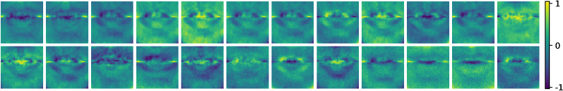
Figure 4: Each one of these 67$\times$67 images visualizes the learned values of the weights associated with a node of the first fully-connected layer of the base V-VAE architecture. This first layer contains 512 nodes, hence there is an equal number of images like the ones displayed here. This illustrates the effectiveness of the proposed model to extract speech features from lips.

A-VAE uses the same architecture as the one described in [20]: both encoder and decoder have a single hidden layer with 128 nodes and hyperbolic tangent activations, consisting of only fully-connected layers. The input dimension of the encoder is $F=513$. The dimension of the latent space is $L=32$. As already mentioned in Section IV and illustrated in Fig. 2, V-VAE shares the same decoder architecture as A-VAE. The encoder is, however, different because of the need of additional visual feature extraction, as described below.

We adopt two architectures for embedding lip ROIs into a feature vector $\mathbf{v}\in\mathbb{R}^{M}$, with $M=128$. The first architecture, base V-VAE, is composed of two fully-connected layers with 512 and 128 nodes, respectively. The dimension of the input corresponds to a single frame that is vectorized, namely $4489=67\times 67$. A fully-connected layer then takes as input the feature vector of dimension $M=128$ and predicts as output the mean and variance parameters in the latent space. The second architecture consists of the base network just described and augmented with a front-end network composed of a 3D convolution layer, that takes as input five consecutive frames and which is constituted of 64 kernels of size $5\times 7\times 7$, followed by batch normalization and rectified linear units, and by a 34 layer ResNet, yielding an output of dimension $1280$ which is then passed to the base network. This front-end network is shown in a dashed box on Fig. 2. The front-end network was trained as part of an AV speech recognition deep architecture [55] using a 500 word vocabulary.

The AV-CVAE architecture is similar to that of A-VAE, except for the fact that the visual features (extracted using one of the two networks described above) are concatenated with the speech-spectrogram time frames at the input of the encoder, as well as with the latent code at the input of the decoder. Note that the visual network just described appears three times, once as part of the prior network for ${\bf z}$ and twice as part of AV-CVAE, hence two training strategies are possible, (i) to constrain these three networks to share the same set of weights, or (ii) to allow a different set of weights for each one of these networks. Through our experiments, we noticed that the former strategy yields better performance that the latter, which also has the advantages of dealing with fewer weights, of a lower chance of overfitting and of a reduced computational cost.

It is worth looking at the learned values of the weights associated with the first fully-connected layer of the base V-VAE architecture. In this case, the input consists of $67\times 67$ lip ROIs which is fed into a layer with 512 nodes. Hence, there are $67\times 67$ weights per node. The trained weights of the first layer of the visual sub-network are multiplied (in an element-wise way) with the input, namely raw lip images. As such, these weights extract important features present in the lip images. These weights give us some insights about how the network exploits the visual data. One can visualize these nodes as an image, e.g. Fig. 4 in which 24 such images are displayed. This illustrates the effectiveness of the proposed V-VAE model to extract salient visual speech features. It can be seen that the shown weights exhibit lip-like shapes. The parts of the weight images with higher intensities correspond to regions on the input lip images that are relevant for the task at hand.

VII-D State of the Art Method

The AV speech enhancement method we propose is unsupervised, i.e. it does not require pairs of clean and noisy speech signals for training. Nevertheless, it is interesting to compare its performance with a supervised method. We compare our approach with the recently proposed state-of-the-art supervised method [15], which is close to the one proposed in [17], and whose Python implementation is publicly available online. This method is based on a DNN made of two subnetworks, one for processing spectrograms of noisy speech and another one for processing lip ROIs. The resulting audio and visual encodings are then concatenated and processed to yield a single embedding which is fed into a network with three fully-connected layers. Finally, a spectrogram of the enhanced speech is obtained using an audio decoder [15].

As is the case with the front-end visual network described above [55], 128$\times$128 frames containing lip ROIs are extracted from the raw video associated with a speaker and the visual input to the network is composed of five consecutive frames. The audio input is a spectrogram synchronized with these five frames. For training, we used the parameter setting suggested by the authors of [15]. Training this supervised method requires noisy mixtures. We used the DEMAND dataset [62] to add various noise types to the clean-speech sequences of the NTCD-TIMIT dataset, with various SNR levels. We used the same SNR levels as in the NTCDT-TIMIT test dataset. The noise types of the DEMAND dataset are different than the ones that were used to generate noisy-speech instances described in Section VII-A, although they share similarities.

In addition to the supervised audio-visual method described above, we also compare the performance of the proposed method with an audio-only NMF baseline. It corresponds to a framework referred to as “semi-supervised source separation” in the literature [63, 64, 39], where during a training phase, we first learn a speech NMF dictionary from a dataset of clean speech signals. Then, at test time, given the learned dictionary, the speech activation matrix and the noise NMF model parameters are estimated from the noisy mixture signals. The speech signal is then estimated by Wiener filtering.

VII-E Implementation Details and Parameter Settings

As mentioned above, VAE training requires a gradient-ascent method. In practice we used the Adam optimizer [65] with a step size of $10^{-4}$. Using the NTCD-TIMIT validation set, early stopping was used with a patience of $20$ epochs. To alleviate the effect of random initialization, we have trained each VAE model five times. The performance was measured by averaging across the sequences present in the dataset (see below) as well as across these five trained models.

The rank of the NMF noise model is set to $K=10$ and the parameters of the nonnegative matrices associated with this model are randomly initialized with nonnegative values. For the baseline NMF method [63], the rank of the NMF speech model is set to $64$. Similarly to [19, 20], at the first iteration of the MCEM algorithm, the Markov chain of the Metropolis-Hastings algorithm was initialized using the mixture signal and the corresponding visual features as input to the encoder. That is, for all $l\in\{0,...,L-1\}$, $z_{ln}^{(0)}=\tilde{\mu}_{l}\left(\tilde{\mathbf{x}}_{n},{\mathbf{v}}_{n}\right)$, where we used the same notation as above, namely $\tilde{\mathbf{x}}_{n}\triangleq(|x_{0n}|^{2}\dots|x_{F-1\>n}|^{2})^{\top}$

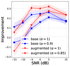
(a) PESQ

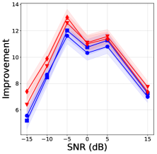
(b) SDR

Figure 5: Performance of AV-CVAE for two different values of $\alpha$ in (12), and for the two variants of visual feature embedding.

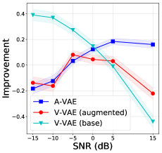
(a) PESQ

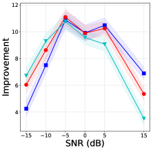
(b) SDR

Figure 6: Performance comparison of A-VAE and of the two variants of V-VAE.

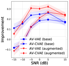
(a) PESQ

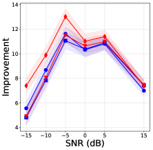
(b) SDR

Figure 7: Performance and comparison of AV-VAE and AV-CVAE.

VII-F Results

We used standard speech enhancement scores, namely the signal-to-distortion ratio (SDR) [66], the perceptual evaluation of speech quality (PESQ) [67], and the short-time objective intelligibility (STOI) scores [68]. SDR is measured in decibels (dB), while PESQ and STOI values lie in the intervals $[-0.5,4.5]$ and $[0,1]$, respectively (the higher the better). For computing SDR the mir_eval Python library was used. For each measure, we report the difference between the output value, i.e., evaluated on the enhanced speech signal, and the input value, i.e., evaluated on the noisy/unprocessed mixture signal.

We compared the proposed unsupervised AV-CVAE method and its variants with the supervised state of the art method outlined above, [15], and the unsupervised NMF method inspired from [63]. For each experiment, the median values of SDR, PESQ, and STOI scores, along with their corresponding standard errors, computed over all noise types, all test samples, and over five models obtained with five random initializations. The SDR, PESQ, and STOI scores are plotted as a function of noise levels.

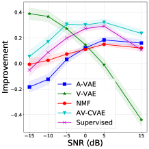
(a) PESQ

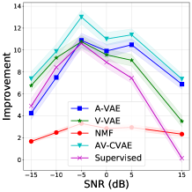
(b) SDR

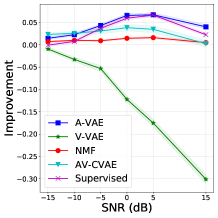
(c) STOI

Figure 8: Performance comparison of A-VAE, V-VAE, NMF, AV-CVAE, and [15] on the test samples from the NTCD-TIMIT dataset.

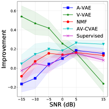
(a) LR

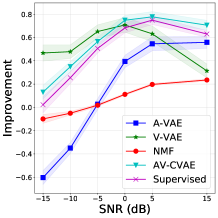
(b) White

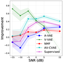
(c) Street

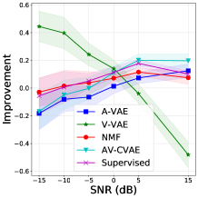
(d) Cafe

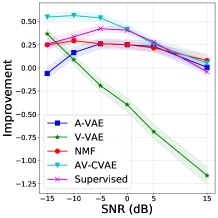
(e) Car

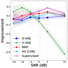
(f) Babble

Figure 9: PESQ results per noise types.

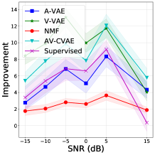
(a) LR

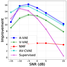
(b) White

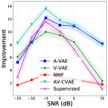
(c) Street

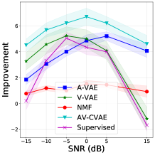
(d) Cafe

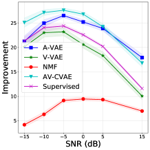
(e) Car

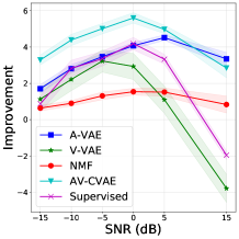
(f) Babble

Figure 10: SDR results per noise types.

We start by comparing the performance of A-VAE with the two V-VAE variants described in Section IV and Section VII-C and illustrated in Fig. 2. The performance scores as a function of noise are shown in Fig. 6. V-VAE performs better than A-VAE when the latter has to deal with high noise levels. One explanation for this could be the initialization of the latent variables in the Markov chain of the Metropolis-Hastings algorithm. In the case of V-VAE, the initialization is based on the visual features, whereas in A-VAE, it is based on the noisy mixture. Consequently, the former provides a better initialization than the latter, as it uses noise-free data (visual features). However, compared with A-VAE, the performance of V-VAE decreases as the noise level decreases. Intuitively, this is expected since the visual input of V-VAE does not depend on the noise associated with the audio signal. This intuition is confirmed by the curves plotted in Fig. 6. From this figure we can also see that the augmented V-VAE performs worse than the base V-VAE for high noise levels, especially in terms of PESQ. This can be explained by the fact that in V-VAE the posterior distribution of the latent variables is learned using only visual data. Therefore, by training from raw visual data, i.e., lip images, the network tries to learn as much as possible from raw visual data to reconstruct the audio data. Pre-trained visual features obtained from the ResNet, on the other hand, may not be as efficient as directly learning from raw visual data. This is because the ResNet has been trained to perform a different task.

Next we assess the performance of AV-CVAE using two values for $\alpha$ in (12): $\alpha=1$ which corresponds to the original ELBO in (10), $\alpha=0.9$ using the base V-VAE network and $\alpha=0.85$ using the augmented V-VAE. The score curves are plotted in Fig. 5 and one can see that the method performs better with $\alpha<1$ than with $\alpha=1$. As explained in Section V, this improvement comes from the reduction of the gap between the prior and the approximate posterior of the AV-CVAE model. In fact, the prior network is trained to generate latent vectors from visual features that are suitable for speech enhancement. In the following we thus use the AV-CVAE network with $\alpha=0.9$.

We also compared the performance of AV-CVAE with AV-VAE. We briefly remind that the former model uses visual information for training the prior, while the latter doesn’t use visual information. Clearly, as it can be seen in Fig. 7, AV-CVAE significantly outperforms AV-VAE, in particular with high noise levels.

In order to assess an overall performance of the proposed algorithms, we compared A-VAE, V-VAE, AV-CVAE, NMF [63], and the state of the art method of [15]. The scores plotted in Fig. 8 show that AV-CVAE outperforms the A-VAE method by more than $2$ dB, in terms of SDR, and by more than $0.3$ in terms of the PESQ score. Moreover, AV-CVAE outperforms [15] by more than $2$dBs (on an average) in terms of SDR and by $0.1$ in terms of PESQ. Nevertheless, A-VAE and [15] outperforms AV-CVAE in terms of STOI for low noise levels. NMF, on the other hand, shows a worse performance than A-VAE and AV-CVAE. However, it outperforms A-VAE in terms of PESQ for high noise levels.

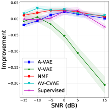
(a) LR

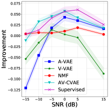
(b) White

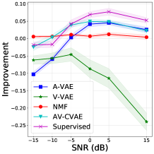
(c) Street

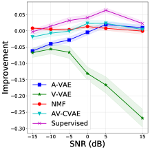
(d) Cafe

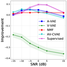
(e) Car

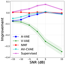
(f) Babble

Figure 11: STOI results per noise types.

To see how the algorithms perform for each different noise type, we have reported the performance scores computed over all test samples, separately for each type of noise. Figures 9, 10, and 11 show the results. As can be seen, the performance ordering of the algorithms is different for each noise type.

Finally, we compared the performance of all the algorithms, trained using the NTCD-TIMIT dataset, on some test samples from the GRID dataset. The scores are shown in Fig. 12, where we can see that AV-CVAE outperforms all the other methods in terms of PESQ (except for low noise levels, which is expected since visual information is less useful as the SNR is increased) and SDR with a significant margin.

It should be emphasized that while the supervised method [15] needs to be trained with various noise types and noise levels, in order to have a good generalization performance, the proposed method is only trained on clean audio-speech and visual-speech samples, independently of noise types and noise levels. However, one advantage of [15] is its computational efficiency at testing. Also, notice that this method takes advantage of the dynamics of both the audio and visual data, through the presence of convolutional layers, which is not the case of our method that used fully-connected layers.

VIII Conclusions

We proposed an audio-visual conditional VAE to model speech prior for speech enhancement. We described in detail several VAE architecture variants and we provided details on how to estimate their parameters. We combined this audio-visual speech prior model with an audio mixture model and with a noise variance model based on NMF. We derived an MCEM algorithm that infers both the time-varying loudness of the speech input and the noise variance parameters. Finally, a probabilistic Wiener filter performs speech reconstruction.

Extensive experiments empirically validate the effectiveness of the proposed methodology to fuse audio and visual inputs for speech enhancement. In particular, the visual modality, i.e. video frames of moving lips, is shown to improve the performance, in particular when the audio modality is highly corrupted with noise.

Future works include the use of recurrent and convolutional layers in order to model temporal dependencies between audio and visual frames, and the investigation of computational efficient inference algorithms. It is also planned to extend the proposed AV-CVAE framework to deal with more realistic visual information, e.g. in the presence of head motions and of temporary occlusions of the lips. Phase-aware speech generative models such as [69] could also be considered for AV speech enhancement.

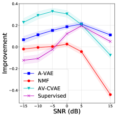
(a) PESQ

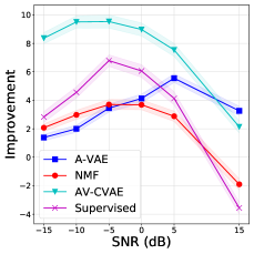
(b) SDR

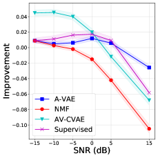
(c) STOI

Figure 12: Performance comparison of A-VAE, NMF, AV-CVAE, and [15] on the GRID dataset. All the models have been trained on the NTCD-TIMIT dataset.

References

- [1] Jae Soo Lim, Speech enhancement, Prentice-Hall Englewood Cliffs, NJ, 1983.
- [2] Jacob Benesty, Shoji Makino, and Jingdong Chen, Speech enhancement, Springer Science & Business Media, 2006.
- [3] Philipos C. Loizou, Speech enhancement: theory and practice, CRC press, 2007.
- [4] William Sumby and Irwin Pollack, “Visual contribution to speech intelligibility in noise,” The Journal of the Acoustical Society of America, vol. 26, no. 2, pp. 212–215, 1954.
- [5] Norman Erber, “Auditory-visual perception of speech,” Journal of Speech and Hearing Disorders, vol. 40, no. 4, pp. 481–492, 1975.
- [6] Alison MacLeod and Quentin Summerfield, “Quantifying the contribution of vision to speech perception in noise,” British Journal of Audiology, vol. 21, no. 2, pp. 131–141, 1987.
- [7] Laurent Girin, Gang Feng, and Jean-Luc Schwartz, “Noisy speech enhancement with filters estimated from the speaker’s lips,” in Proc. European Conference on Speech Communication and Technology (EUROSPEECH), Madrid, Spain, 1995, pp. 1559–1562.
- [8] Laurent Girin, Jean-Luc Schwartz, and Gang Feng, “Audio-visual enhancement of speech in noise,” The Journal of the Acoustical Society of America, vol. 109, no. 6, pp. 3007–3020, 2001.
- [9] John W. Fisher III, Trevor Darrell, William T. Freeman, and Paul A. Viola, “Learning joint statistical models for audio-visual fusion and segregation,” in Proc. Advances in Neural Information Processing Systems (NIPS), 2001, pp. 772–778.
- [10] Sabine Deligne, Gerasimos Potamianos, and Chalapathy Neti, “Audio-visual speech enhancement with AVCDCN (audio-visual codebook dependent cepstral normalization),” in Proc. IEEE International Workshop on Sensor Array and Multichannel Signal Processing, 2002, pp. 68–71.
- [11] Roland Goecke, Gerasimos Potamianos, and Chalapathy Neti, “Noisy audio feature enhancement using audio-visual speech data,” in Proc. IEEE International Conference on Acoustics, Speech, and Signal Processing (ICASSP), 2002, pp. II–2025–2028.
- [12] John R. Hershey and Michael Casey, “Audio-visual sound separation via hidden Markov models,” in Proc. Advances in Neural Information Processing Systems (NIPS), 2002, pp. 1173–1180.
- [13] Ahmed Hussen Abdelaziz, Steffen Zeiler, and Dorothea Kolossa, “Twin-HMM-based audio-visual speech enhancement,” in Proc. IEEE International Conference on Acoustics, Speech and Signal Processing (ICASSP), 2013, pp. 3726–3730.
- [14] Triantafyllos Afouras, Joon Son Chung, and Andrew Zisserman, “The conversation: Deep audio-visual speech enhancement,” in Proc. Conference of the International Speech Communication Association (INTERSPEECH), 2018, pp. 3244–3248.
- [15] Aviv Gabbay, Asaph Shamir, and Shmuel Peleg, “Visual speech enhancement,” in Proc. Conference of the International Speech Communication Association (INTERSPEECH), 2018, pp. 1170–1174.
- [16] Aviv Gabbay, Ariel Ephart, Tavi Halperin, and Shmuel Peleg, “Seeing through noise: Speaker separation and enhancement using visually-derived speech,” in Proc. IEEE International Conference on Acoustics, Speech, and Signal Processing (ICASSP), 2018, pp. 3051–3055.
- [17] Jen-Cheng Hou, Syu-Siang Wang, Ying-Hui Lai, Yu Tsao, Hsiu-Wen Chang, and Hsin-Min Wang, “Audio-visual speech enhancement using multimodal deep convolutional neural networks,” IEEE Transactions on Emerging Topics in Computational Intelligence, vol. 2, no. 2, pp. 117–128, 2018.
- [18] Mandar Gogate, Ahsan Adeel, Ricard Marxer, Jon Barker, and Amir Hussain, “DNN driven speaker independent audio-visual mask estimation for speech separation,” in Proc. Conference of the International Speech Communication Association (INTERSPEECH), 2018, pp. 2723–2727.
- [19] Yoshiaki Bando, Masato Mimura, Katsutoshi Itoyama, Kazuyoshi Yoshii, and Tatsuya Kawahara, “Statistical speech enhancement based on probabilistic integration of variational autoencoder and non-negative matrix factorization,” in Proc. IEEE International Conference on Acoustics, Speech, and Signal Processing (ICASSP), 2018, pp. 716–720.
- [20] Simon Leglaive, Laurent Girin, and Radu Horaud, “A variance modeling framework based on variational autoencoders for speech enhancement,” in Proc. IEEE International Workshop on Machine Learning for Signal Processing (MLSP), 2018, pp. 1–6.
- [21] Kouhei Sekiguchi, Yoshiaki Bando, Kazuyoshi Yoshii, and Tatsuya Kawahara, “Bayesian multichannel speech enhancement with a deep speech prior,” in Proc. Asia-Pacific Signal and Information Processing Association Annual Summit and Conference (APSIPA ASC), 2018, pp. 1233–1239.
- [22] Simon Leglaive, Laurent Girin, and Radu Horaud, “Semi-supervised multichannel speech enhancement with variational autoencoders and non-negative matrix factorization,” in Proc. IEEE International Conference on Acoustics, Speech, and Signal Processing (ICASSP), 2019, pp. 101–105.
- [23] Simon Leglaive, Umut Şimşekli, Antoine Liutkus, Laurent Girin, and Radu Horaud, “Speech enhancement with variational autoencoders and alpha-stable distributions,” in Proc. IEEE International Conference on Acoustics, Speech, and Signal Processing (ICASSP), 2019, pp. 541–545.
- [24] Manuel Pariente, Antoine Deleforge, and Emmanuel Vincent, “A statistically principled and computationally efficient approach to speech enhancement using variational autoencoders,” in Proc. Conference of the International Speech Communication Association (INTERSPEECH), 2019.
- [25] Kihyuk Sohn, Honglak Lee, and Xinchen Yan, “Learning structured output representation using deep conditional generative models,” in Proc. Advances in Neural Information Processing Systems (NIPS), 2015, pp. 3483–3491.
- [26] Xiaofei Li and Radu Horaud, “Multichannel speech enhancement based on time-frequency masking using subband long short-term memory,” in IEEE Workshop on Applications of Signal Processing to Audio and Acoustics. IEEE, 2019, pp. 298–302.
- [27] Ahmed Hussen Abdelaziz, “NTCD-TIMIT: A new database and baseline for noise-robust audio-visual speech recognition,” in Proc. Conference of the International Speech Communication Association (INTERSPEECH), 2017, pp. 3752–3756.
- [28] Martin Cooke, Jon Barker, Stuart Cunningham, and Xu Shao, “An audiovisual corpus for speech perception and automatic speech recognition,” J. Acoustical Society of America, vol. 120, no. 5, pp. 2421–2424, 2006.
- [29] Steven Boll, “Suppression of acoustic noise in speech using spectral subtraction,” IEEE Transactions on Acoustics, Speech, and Signal Processing, vol. 27, no. 2, pp. 113–120, 1979.
- [30] Jae Soo Lim and Alan V Oppenheim, “Enhancement and bandwidth compression of noisy speech,” Proceedings of the IEEE, vol. 67, no. 12, pp. 1586–1604, 1979.
- [31] Yariv Ephraim and David Malah, “Speech enhancement using a minimum-mean square error short-time spectral amplitude estimator,” IEEE Transactions on Acoustics, Speech, and Signal Processing, vol. 32, no. 6, pp. 1109–1121, 1984.
- [32] Rainer Martin, “Speech enhancement based on minimum mean-square error estimation and supergaussian priors,” IEEE Transactions on Speech and Audio Processing, vol. 13, no. 5, pp. 845–856, 2005.
- [33] Jan Erkelens, Richard Hendriks, Richard Heusdens, and Jesper Jensen, “Minimum mean-square error estimation of discrete Fourier coefficients with generalized Gamma priors,” IEEE Transactions on Audio, Speech, and Language Processing, vol. 15, no. 6, pp. 1741–1752, 2007.
- [34] Yariv Ephraim and David Malah, “Speech enhancement using a minimum mean-square error log-spectral amplitude estimator,” IEEE Transactions on Acoustics, Speech, and Signal Processing, vol. 33, no. 2, pp. 443–445, 1985.
- [35] Israel Cohen and Baruch Berdugo, “Speech enhancement for non-stationary noise environments,” Signal processing, vol. 81, no. 11, pp. 2403–2418, 2001.
- [36] Cédric Févotte, Nancy Bertin, and Jean-Louis Durrieu, “Nonnegative matrix factorization with the Itakura-Saito divergence: With application to music analysis,” Neural computation, vol. 21, no. 3, pp. 793–830, 2009.
- [37] Kevin Wilson, Bhiksha Raj, Paris Smaragdis, and Ajay Divakaran, “Speech denoising using nonnegative matrix factorization with priors,” in Proc. IEEE International Conference on Acoustics, Speech and Signal Processing (ICASSP), Las Vegas, USA, 2008, pp. 4029–4032.
- [38] Bhiksha Raj, Rita Singh, and Tuomas Virtanen, “Phoneme-dependent NMF for speech enhancement in monaural mixtures,” in Proc. Conference of the International Speech Communication Association (INTERSPEECH), 2011, pp. 1217–1220.
- [39] Nasser Mohammadiha, Paris Smaragdis, and Arne Leijon, “Supervised and unsupervised speech enhancement using nonnegative matrix factorization,” IEEE Transactions on Audio, Speech, and Language Processing, vol. 21, no. 10, pp. 2140–2151, 2013.
- [40] DeLiang Wang and Jitong Chen, “Supervised speech separation based on deep learning: An overview,” IEEE Transactions on Audio, Speech, and Language Processing, vol. 26, no. 10, pp. 1702–1726, 2018.
- [41] Xugang Lu, Yu Tsao, Shigeki Matsuda, and Chiori Hori, “Speech enhancement based on deep denoising autoencoder.,” in Proc. Conference of the International Speech Communication Association (INTERSPEECH), 2013, pp. 436–440.
- [42] Yong Xu, Jun Du, Li-Rong Dai, and Chin-Hui Lee, “A regression approach to speech enhancement based on deep neural networks,” IEEE Transactions on Audio, Speech, and Language Processing, vol. 23, no. 1, pp. 7–19, 2015.
- [43] Szu-Wei Fu, Yu Tsao, and Xugang Lu, “SNR-aware convolutional neural network modeling for speech enhancement.,” in Proc. Conference of the International Speech Communication Association (INTERSPEECH), 2016, pp. 3768–3772.
- [44] Yuxuan Wang and DeLiang Wang, “Towards scaling up classification-based speech separation,” IEEE Transactions on Audio, Speech, and Language Processing, vol. 21, no. 7, pp. 1381–1390, 2013.
- [45] Yuxuan Wang, Arun Narayanan, and DeLiang Wang, “On training targets for supervised speech separation,” IEEE/ACM transactions on audio, speech, and language processing, vol. 22, no. 12, pp. 1849–1858, 2014.
- [46] Felix Weninger, Hakan Erdogan, Shinji Watanabe, Emmanuel Vincent, Jonathan Le Roux, John R Hershey, and Björn Schuller, “Speech enhancement with LSTM recurrent neural networks and its application to noise-robust ASR,” in Proc. International Conference on Latent Variable Analysis and Signal Separation (LVA/ICA), 2015, pp. 91–99.
- [47] Diederik. P. Kingma, Danilo J. Rezende, Shakir Mohamedy, and Max Welling, “Semi-supervised learning with deep generative models,” in Adv. Neural Information Processing Systems (NIPS), 2014, pp. 3581–3589.
- [48] Hirokazu Kameoka, Li Li, Shota Inoue, and Shoji Makino, “Supervised determined source separation with multichannel variational autoencoder,” Neural Computation, vol. 31, no. 9, pp. 1–24, 2019.
- [49] Li Li, Hirokazu Kameoka, and Shoji Makino, “Fast MVAE: Joint separation and classification of mixed sources based on multichannel variational autoencoder with auxiliary classifier,” in Proc. IEEE International Conference on Acoustics, Speech, and Signal Processing (ICASSP), 2019, pp. 546–550.
- [50] Shota Inoue, Hirokazu Kameoka, Li Li, Shogo Seki, and Shoji Makino, “Joint separation and dereverberation of reverberant mixtures with multichannel variational autoencoder,” in Proc. IEEE International Conference on Acoustics, Speech, and Signal Processing (ICASSP), 2019, pp. 96–100.
- [51] Ibrahim Almajai and Ben Milner, “Visually derived wiener filters for speech enhancement,” IEEE Transactions on Audio, Speech, and Language Processing, vol. 19, no. 6, pp. 1642–1651, 2010.
- [52] Greg C.G. Wei and Martin A. Tanner, “A Monte Carlo implementation of the EM algorithm and the poor man’s data augmentation algorithms,” Journal of the American statistical Association, vol. 85, no. 411, pp. 699–704, 1990.
- [53] Michael I. Jordan, Zoubin Ghahramani, Tommi S. Jaakkola, and Lawrence K. Saul, “An introduction to variational methods for graphical models,” Machine learning, vol. 37, no. 2, pp. 183–233, 1999.
- [54] David M. Blei, Alp Kucukelbir, and Jon D. McAuliffe, “Variational inference: A review for statisticians,” Journal of the American Statistical Association, vol. 112, no. 518, pp. 859–877, 2017.
- [55] Stavros Petridis, Themos Stafylakis, Pingchuan Ma, Feipeng Cai, Georgios Tzimiropoulos, and Maja Pantic, “End-to-end audiovisual speech recognition,” in Proc. IEEE International Conference on Acoustics, Speech, and Signal Processing (ICASSP), 2018, pp. 6548–6552.
- [56] Irina Higgins, Loic Matthey, Arka Pal, Christopher Burgess, Xavier Glorot, Matthew Botvinick, Shakir Mohamed, and Alexander Lerchner, “-vae: Learning basic visual concepts with a constrained variational framework,” in International Conference on Learning Representations (ICLR), 2017.
- [57] Arthur P. Dempster, Nan M. Laird, and Donald B. Rubin, “Maximum likelihood from incomplete data via the EM algorithm,” Journal of the royal statistical society. Series B (Methodological), vol. 39, no. 1, pp. 1–38, 1977.
- [58] Christian P. Robert and George Casella, Monte Carlo Statistical Methods, Springer-Verlag New York, Inc., Secaucus, NJ, USA, 2005.
- [59] Cédric Févotte and Jérôme Idier, “Algorithms for nonnegative matrix factorization with the -divergence,” Neural computation, vol. 23, no. 9, pp. 2421–2456, 2011.
- [60] John S. Garofolo, Lori F. Lamel, William M. Fisher, Jonathan G. Fiscus, David S. Pallett, Nancy L. Dahlgren, and Victor Zue, “TIMIT acoustic phonetic continuous speech corpus,” in Linguistic data consortium, 1993.
- [61] Hans-Günter Hirsch, “FaNT– filtering and noise adding tool,” Tech. Rep., International Computer Science Institute, Niederrhein University of Applied Science, 2005.
- [62] Joachim Thiemann, Nobutaka Ito, and Emmanuel Vincent, “The Diverse Environments Multi-channel Acoustic Noise Database (DEMAND): A database of multichannel environmental noise recordings,” in Proc. International Congress on Acoustics, 2013.
- [63] Paris Smaragdis, Bhiksha Raj, and Madhusudana Shashanka, “Supervised and semi-supervised separation of sounds from single-channel mixtures,” in Proc. Int. Conf. Indep. Component Analysis and Signal Separation, 2007, pp. 414–421.
- [64] Gautham J. Mysore and Paris Smaragdis, “A non-negative approach to semi-supervised separation of speech from noise with the use of temporal dynamics,” in 2011 IEEE International Conference on Acoustics, Speech and Signal Processing (ICASSP), 2011.
- [65] Diederik P. Kingma and Jimmy Ba, “Adam: A method for stochastic optimization,” in International Conference on Learning Representations (ICLR), 2015.
- [66] Emmanuel Vincent, Rémi Gribonval, and Cédric Févotte, “Performance measurement in blind audio source separation,” IEEE Transactions on Audio, Speech, and Language Processing, vol. 14, no. 4, pp. 1462–1469, 2006.
- [67] Antony W. Rix, John G. Beerends, Michael P. Hollier, and Andries P. Hekstra, “Perceptual evaluation of speech quality (PESQ)-a new method for speech quality assessment of telephone networks and codecs,” in Proc. IEEE International Conference on Acoustics, Speech, and Signal Processing (ICASSP), 2001, pp. 749–752.
- [68] Cees H. Taal, Richard C. Hendriks, Richard Heusdens, and Jesper Jensen, “An algorithm for intelligibility prediction of time–frequency weighted noisy speech,” IEEE Trans. Audio, Speech, Language Process., vol. 19, no. 7, pp. 2125–2136, 2011.
- [69] Aditya Arie Nugraha, Kouhei Sekiguchi, and Kazuyoshi Yoshii, “A deep generative model of speech complex spectrograms,” in Proc. IEEE International Conference on Acoustics, Speech, and Signal Processing (ICASSP), 2019, pp. 905–909.