Free-Lunch Saliency via Attention in Atari Agents

Abstract

We propose a new approach to visualize saliency maps for deep neural network models and apply it to deep reinforcement learning agents trained on Atari environments. Our method adds an attention module that we call FLS (Free Lunch Saliency) to the feature extractor from an established baseline [24]. This addition results in a trainable model that can produce saliency maps, i.e., visualizations of the importance of different parts of the input for the agent’s current decision making. We show experimentally that a network with an FLS module exhibits performance similar to the baseline (i.e., it is “free”, with no performance cost) and can be used as a drop-in replacement for reinforcement learning agents. We also design another feature extractor that scores slightly lower but provides higher-fidelity visualizations. In addition to attained scores, we report saliency metrics evaluated on the Atari-HEAD dataset of human gameplay.

1 Introduction

Reinforcement learning (RL) models train agents that process input information from the environment in order to learn and implement a policy that maximizes the desired reward [39]. Over the last decade, reinforcement learning has shifted towards deep reinforcement learning, where policies and/or models of the environment are modeled with deep neural networks, with impressive results achieved across a wide variety of tasks, from game playing to robotics [2, 14]. Unfortunately, both RL and deep learning in general suffer from poor interpretability: it is hard to explain why a deep neural network performs as it does, hard to understand why an RL agent has assigned a specific value to a given state, and harder yet when these two inherently “black-box” methods come together [8]. On the other hand, interpretability is a key feature for many critical applications, especially in robotics. This motivates the design of interpretable RL agents and modifying existing architectures for easier interpretation.

In this work, we concentrate on RL problems where the environment is represented by an image; a common example is given by Atari game environments popularized for deep RL in [23]. In this context, interpretability often comes in the form of saliency maps, i.e., values of how important individual pixels or small patches of the input image are for the Q-function or current policy decision. In the context of deep convolutional networks, saliency maps were introduced in [34], where gradients of the output category for image classification problems were visualized with respect to the input components (pixels). A map of such values provides some intuition of pixel importance: large absolute values of the gradients tell us that changes in those pixels can significantly affect the output category. Later works shifted the focus from trying to interpret already trained models towards building interpretability into the models themselves, usually with some form of an attention mechanism [4]; we give a survey of these and other methods in Section 2. However, adding built-in interpretability often leads to a significant decrease in the actual rewards obtained by the resulting RL agents, i.e., usually one can have either state of the art performance or interpretability but not both.

We aim to explore the possibility of having both interpretable visualizations and high rewards at the same time. We introduce a visualization layer used to change the feature extractor’s architecture in such a way that it learns visualizations as a side effect of training. We conduct a comprehensive experimental study on six Atari environments: BeamRider, Breakout, MsPacman, SpaceInvaders, Enduro, and Seaquest. As a result of applying soft attention to Atari gameplay screenshots (adding a new layer), the resulting agent is able to localize its attention and generate saliency maps in the process of training. These saliency maps can be used to understand how the agent learns. Moreover, they provide a close match to human attention. To evaluate this effect, we have used the Atari Human Eye-Tracking and Demonstration Dataset (Atari-HEAD) [45] as the ground truth, measuring the similarity between saliency maps and human eye movements across three metrics: normalized scanpath saliency (NSS), KL divergence, and shuffled AUC.

Thus, we present a useful and interpretable way for visualization. Unlike other ways of visualizing the agents’ performance, such as Jacobians or reward curves [40], saliency maps can allow even non-experts to draw reasonable conclusions. Moreover, it provides an easy way for debugging agents and interpreting the policy.

The paper is organized as follows. In Section 2, we provide an overview of different ways to improve the interpretability of deep RL models and agents. Section 3 introduces our attention-based modifications to the baseline RL agents and previously developed models. A comprehensive evaluation study of our model against these competitors is provided in Section 4. We speculate on potential avenues for future research and conclude the paper in Section 5.

2 Related work

In this section, we review the recent interpretability and saliency studies in deep reinforcement learning (RL). Since we had been unable to find comprehensive surveys of existing work to reference during literature review, we decided to make this section into such a review. The deep RL revolution was started by [23], who successfully used deep CNNs trained using Q-learning to play Atari games from raw pixels. In a follow-up work [24] they were also the first to attempt to interpret trained models by applying t-SNE to network hidden states. They used a single architecture to play all of the environments. We show its feature extractor in Figure 2.a, with the corresponding Sparse block in Figure 1.a. We broadly divide work on interpreting deep RL models and deep neural networks in general into two major categories: post-hoc and built-in saliency. Next, we briefly review the former and provide a comprehensive survey of the latter.

Post-hoc saliency

includes approaches where additional techniques intended for interpretation follow an already trained model, without affecting the model and the training process itself.

As we have already noted, saliency maps were first introduced in deep learning in the context of image classification by [34], who proposed to visualize gradients of output category with respect to input image. This general approach was extended in many later works, most notably with guided backpropagation [37], integrated gradients [38], Grad-CAM [31], LRP [3], and DeepLIFT [33]. The current state of the art approaches are SmoothGrad [35] and VarGrad [1], which were studied theoretically in [32] and found to be best in a recent comprehensive evaluation [20].

In the context of deep RL in particular, studies of interpretability were pioneered by [24] who applied t-SNE to a CNN network playing Atari games; later, Jacobians of value and advantage streams with respect to input images were used for the same purpose in [40]. The work [44] investigated t-SNE embeddings in more depth. In [15], saliency maps for Atari agents trained with A3C were visualized by blurring different parts of input images and measuring the $L^{2}$ difference between actor and critic outputs; such an approach is computationally expensive but the resulting images are clearer than Jacobians. Recently, the work [41] took a closer look at a slightly modified version of Grad-CAM in the context of deep RL on Atari games.

Built-in saliency

refers to approaches where interpretability follows from special constructions added to the models themselves. There is already a significant number of works in this direction. We give a brief summary of their main features in Table 1 and describe them in more detail below.

Ref	Algorithm	Custom env	# envs (Atari)	Based on	Train- able attn	Attention types	Attention architecture	Sum- pool	Vis. method	Metrics
[36]	DRQN	✗	5	[17]	✓	Soft and hard self-attention	Fig. 1.d	✓	Upscale	Reward
[9]	DRQN	✗	3	[17]	✓	Soft temporal and spatial self-attention	Fig. 1.d	✓	Upscale*	Reward
[26]	DRQN	✗	5	[17]	✓	Soft self-attention	Fig. 1.e	✓	Upscale*	NSS, AUC
[10]	DQN	GridWorld	0	Custom	✓	Soft key-value	See [10]	✓	Raw	Reward
[46]	Imitation	✗	8	[24]	✓	Soft, on human data	See [46]	N/A	Raw	Reward, NSS, AUC, KL, CC
[43]	A2C	Catch	4	[24]	✗	N/A	N/A	N/A	Opt. flow	Reward
[42]	Rainbow	✗	8	[24]	✓	Soft	Fig. 1.c	✗	Jacobian	Reward
[22]	PPO	✗	10	[24]	✓	Soft self-attention	*	✗	Grad-CAM + upscale	Reward
[25]	IMPALA	✗	57	[13]	✓	Soft key-value	See [25]	✓	Raw	Reward
Ours	PPO	✗	6	[24], custom	✓	Soft self-attention	Fig. 1.f	both	$\mathrm{conv}^{T}$	Reward, NSS, KL, sAUC

Table 1: Papers on ad-hoc saliency. Asterisks show cases where the original paper is vague on exact details.

One of the first notable models with saliency in RL via attention is DARQN [36] (Figure 1.d), a modification of DRQN [17] augmented with spatial attention dependent on the recurrent state. The authors experimented with both soft attention (regular spatial attention) and hard attention (sampling from the distribution generated by the attention network). The results are ambiguous: while achieving high scores on Seaquest, they scored lower than baseline scores on Breakout. We compare our approach against a non-recurrent variation of their method, which we call DAQN.

In [9], a similar approach is augmented by experiments with temporal attention in addition to spatial attention. Despite the fact that temporal attention appears to improve performance, it cannot be used to obtain saliency maps, so we do not consider it in our work. The work [9] is vague on the exact procedure for obtaining visualizations, although they look like simple upscalings of attention activations.

The work [26] refers to assessors in order to get areas of the input image (frame) which people are most likely to look at during a game. The collected data is used as a proxy for gaze positions. Comparing to previous works, the model is trained with a smaller attention module, and the resulting saliency maps are evaluated by measuring how similar they are to data collected from humans. The authors compare their approach with two methods for determining saliency that are not based on DL: Itti-Koch saliency model [21] and Graph-Based Visual Saliency (GBVS) [16]. They show that both of them are no better than random, while attention-based saliency significantly outperforms them. They also do not specify their visualization method precisely.

The work [46] also uses human attention data but brings a different approach: they have collected a dataset of human gaze positions with an eye tracker, trained an encoder-decoder architecture to predict human gaze positions using that data, and finally used it to train an agent with imitation learning, achieving promising results.

The approach of [42] is very similar to ours: their main modification is the addition of a custom attention block (Figure 2.c) that they call RS (Region-Sensitive) module. They train the resulting model with Rainbow [19] and show that the it learns to focus its attention on semantically relevant areas. The work [22] tested variations of self-attention but used Grad-CAM to visualize saliency maps.

Inspired by selective attention models, the authors of [43] use optical flow between two frames as the attention map. They experiment with A2C on Atari games, conducting several experiments on DQN with and without attention and reporting moderate performance improvements on four Atari games (Breakout, Seaquest, MsPacman, and Centipede). However, they provide no metrics or ways to estimate the result quantitatively. The authors remark that more experimental data is needed to show the benefits of visual attention for deep RL models, stating that “experiments on more games should be conducted to provide a more comprehensive evaluation for the effect of introducing visual attention”.

In [10], an attention model is applied to a toy problem in single-agent and multi-agent settings. The authors show better performance compared to the DQN and report advantages of a multi-agent architecture over a single-agent one. Furthermore, they report 20% better sample efficiency.

In a recent paper [25], soft top-down attention in a recurrent model is used to force the agent to focus on task-relevant information. The resulting agent exhibits performance comparable to state of the art on Atari games.

3 Our approach

Figure 1: Convolutional and attention blocks. At time $t$, input frames $s_{t}$ are turned into embeddings $v_{t}$, $h_{t}$ is the recurrent state: (a) Sparse convolutional block; (b) Dense convolutional block; (c) Region-Sensitive Module [42]; (d) DARQN [36] ($N=256$) and [9] ($N=512$); (e) architecture from [26]; (f) our architecture ($h_{t}\equiv 0$).

Figure 2: Model architectures; $s_{t}$ – input frames at time $t$: (a) Nature CNN [24]; (b) DAQN, inspired by [36]; (c) LTIAA [42]; (d) our architecture. Fig. 1 shows the Sparse and Dense blocks and attention modules.

Our work continues the general idea of applying attention improvements to RL agents in order to get interpretability while hopefully not sacrificing performance. Unlike all works discussed in Section 2, we suggest a quantitative way to evaluate attention maps produced by the models, using the information from an eye-tracker recently made available in the Atari Human Eye-Tracking and Demonstration Dataset (Atari-HEAD) [45]. This allows us to compare multiple architectures and model setups in order to find the best way of introducing attention to deep RL models.

Contrary to some of the prior art, the Sparse FLS architecture we propose in our work is a small, incremental change from the non-recurrent baseline. We conduct experiments using 5 random seeds across 6 Atari environments, and in all of our experiments, our model performs similarly to the baseline, while also producing visualizations. We also compute saliency metrics using the Atari-HEAD dataset [46] of human eye fixations captured using an eye tracker from human players playing Atari games, showing that neural models perform significantly better than random in approximating human gazes. Finally, we also propose a Dense FLS architecture, which, despite attaining lower scores, generates significantly sharper images.

Deep RL models are notorious for their sensitivity to hyperparameters [18]. For this reason, we primarily investigate incremental changes to approaches that are known to work well [23, 24] rather than attempt to build a new one from scratch. Since post-hoc saliency methods have been studied quite extensively (see Section 2), we develop a model that has built-in saliency. We turn to the idea of attention [4], and, borrowing elements from [27], integrate visual soft self-attention into a baseline model from [24]. We show details of the architectures in Figure 2.

Similar to [42] (Fig. 2.c with the RS module detailed in Fig. 1.c; see Section 2), we add an extra self-attention module between convolutional and fully-connected layers. One of the main differences is that we use SoftPlus [12] as the activation function for the final layer of the FLS module. The choice of SoftPlus is inspired by [27] and motivated by the fact that, in contrast to previous approaches [36, 9, 26, 42], it does not use any normalization. We have verified experimentally that normalizing the output of SoftPlus makes the model perform worse (see Section 4.2). We have also seen that adding sum-pooling makes the model perform worse.

In addition to the Sparse block which is a part of the baseline model from [24], we also propose a different convolutional block which we call Dense, as shown in Fig. 1. It is designed in such a way that the receptive fields and strides of neurons in its final layer are small, making visualizations crisper; but, as we will see in experiments, this comes at the cost of the achieved reward. This model can only reasonably fit in GPU memory if sum-pooling is applied after attention.

We visualize saliency maps generated by FLS modules by drawing receptive fields of all neurons from the final convolutional layer with intensity proportional to the activations of the corresponding neurons in the attention layer, which we implement via transposed convolution of the output of the FLS module with a unit kernel (i.e., a tensor filled with ones) with suitable kernel size, strides, and padding. This approach strikes the balance between bilinear upscaling of the attention activations and more mathematically sound but extremely noisy Jacobian of the input image with respect to some function of attention activations.

In the next section, we proceed to show direct experimental comparisons against the architecture from [42] trained with PPO (which we call RS-PPO) and a non-recurrent version of [36] (denoted DAQN).

4 Experimental evaluation

4.1 Setup

We run all experiments on 6 Atari games [5]: BeamRider, Breakout, MsPacman, SpaceInvaders, Enduro, and Seaquest. This is identical to the set of games reported in an early version of [42] (a later version added Frostbite) with the exception that we replaced Pong with Breakout because in Pong, the score is capped at 21, and it is relatively easy to train an agent that achieves perfect or near-perfect score, which trivializes many comparisons. We use environments provided by the OpenAI Gym library [7], specifically their NoFrameskip-v4 versions.

All agents were trained using the Proximal Policy Optimization (PPO) algorithm [30] as implemented in the OpenAI Baselines library [11], with default hyperparameters. We ran 8 environments in parallel and capped the total number of environment steps at $5\cdot 10^{7}$ to limit resource usage.

For each environment and each architecture, we trained 5 agents with different random seeds. For every experiment, we recorded a smoothed curve of episode rewards the agents obtained during training. Reward curves in Figure 3 show the mean score and its standard deviation on every timestep. Specifically, we show the eprewmean metric reported by the Baselines library and computed as follows: during training, collecting experience is interleaved with agent updates. Experience is collected in 8 threads, which, under default hyperparameters, are executed for 128 steps at a time, totaling 1024 environment steps between agent updates. The eprewmean metric is the average reward for the last 100 episodes completed by the time the experience collection step is over. This includes episodes that are completed in steps prior to the current one. We have made the source code for the implementation of our models and reproducing the experiments available at https://github.com/dniku/free-lunch-saliency.

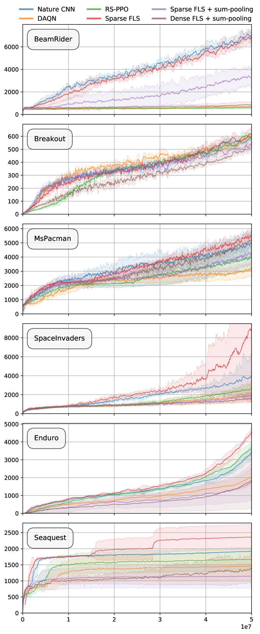
Figure 3: Reward curves during training. The horizontal axis shows the number of environment frames, the vertical axis shows the current reward.

Model	# params	% of [24]
Nature CNN [24]	1,686,693	100%
DAQN [36]	130,726	7.8%
RS-PPO [42]	1,720,999	102.0%
Sparse FLS	1,836,710	108.9%
Sparse FLS + sum-pooling	263,846	15.6%
Dense FLS + sum-pooling	280,358	16.6%
Sparse + FLS after first conv layer	1,762,982	104.5%
Sparse + FLS after each conv layer	2,063,016	122.3%

Table 2: Model sizes. Colors correspond to Fig. 3.

4.2 Performance

Figure 3 shows reward curves obtained during training. It can be seen that our Sparse FLS architecture, which is the baseline model with an extra attention module, performs similarly to the baseline, while our Dense FLS architecture achieves lower rewards. We evaluate each trained model $2^{13}=8192$ times on environments initialized with a previously unseen random seed.

Game	BeamRider	Breakout	Enduro	MsPacman	Seaquest	SpaceInvaders
Nature CNN [24]	6949$\pm$2569	618$\pm$209	3808$\pm$1670	4874$\pm$1701	1920$\pm$37	3867$\pm$3627
DAQN [36]	701$\pm$205	601$\pm$201	2182$\pm$1075	3111$\pm$1165	1453$\pm$420	2096$\pm$1554
RS-PPO [42]	583$\pm$185	605$\pm$202	3851$\pm$1677	3943$\pm$1435	1670$\pm$372	2562$\pm$1339
RS-PPO [42] w/o padding	823$\pm$432	591$\pm$199	3658$\pm$1670	3950$\pm$1371	1710$\pm$379	2248$\pm$782
Sparse FLS	6634$\pm$2361	624$\pm$211	5094$\pm$1876	5421$\pm$1517	2440$\pm$382	9359$\pm$13230
Sparse FLS + sum-pooling	3356$\pm$1878	520$\pm$183	1917$\pm$1486	4317$\pm$1485	1150$\pm$385	1847$\pm$773
Sparse FLS + norm	6584$\pm$2159	598$\pm$200	4524$\pm$1807	3409$\pm$1275	1161$\pm$348	11206$\pm$10441
Sparse FLS w/ $1\times 1$ convs	6870$\pm$2413	621$\pm$207	4701$\pm$1880	4887$\pm$1589	2252$\pm$336	5673$\pm$6344
Sparse FLS w/ $\operatorname{SoftPlus}_{2}$	6697$\pm$2261	612$\pm$208	4854$\pm$1823	5242$\pm$1527	1908$\pm$29	6443$\pm$7684
Sparse FLS w/o final ReLU	6777$\pm$2242	589$\pm$207	4814$\pm$1904	5049$\pm$1145	2013$\pm$185	2929$\pm$556
Sparse FLS w/o final ReLU + sum-pooling	1057$\pm$1061	480$\pm$158	2093$\pm$1469	3365$\pm$1292	2356$\pm$1874	1999$\pm$899
Sparse + FLS after first conv layer	7468$\pm$2645	640$\pm$212	4942$\pm$2053	4720$\pm$1455	2181$\pm$376	9395$\pm$13615
Sparse + FLS after each conv layer	6588$\pm$2348	633$\pm$217	5950$\pm$3739	4978$\pm$1461	2083$\pm$314	2855$\pm$194
Dense FLS + sum-pooling	866$\pm$415	532$\pm$173	2114$\pm$2164	4977$\pm$1253	1368$\pm$517	1549$\pm$831
Dense FLS w/o final ReLU + sum-pooling	730$\pm$245	503$\pm$162	1292$\pm$1829	4879$\pm$1282	10052$\pm$11853	1316$\pm$813

Table 3: Evaluation scores. We trained 5 models with different random seeds for each (game, architecture) pair. Each model was evaluated $8192$ times on environments initialized with a previously unseen random seed, with results aggregated across models. Colors correspond to Fig. 3.

The final results are shown in Table 3. In addition to testing the architectures discussed in Section 3, Table 3 also shows an ablation study and the results of testing several variations intended to verify our hypotheses.

First, we hypothesize that inferior performance of our Dense FLS model is at least partially due to spatial sum-pooling; we test this hypothesis by training an intermediate model, one with a Sparse block and spatial sum-pooling. Experimental results validate our hypothesis, showing much lower results for this intermediate model compared with the regular Sparse-based model. The loss of performance from sum-pooling may be caused by the loss of spatial information (i.e., the position of the ball and paddle in Breakout). Indeed, the work [25] suggests to concatenate fixed Fourier basis vectors to the tensor before applying spatial sum-pooling. We have not investigated the effects of similar workarounds. Note, however, that our Sparse FLS architecture has approximately 10% more parameters than the baseline, while the addition of sum-pooling reduces the number of parameters in the model by nearly a factor of 7 (see Table 2). Thus, in some applications sum-pooling may be a sensible choice in terms of the memory-performance trade-off.

Second, we hypothesize that normalizing the output of the FLS module makes the model perform worse, and train a model where we divide the output of the FLS module by its sum. This, again, reduces the performance, yielding evidence in favor of this hypothesis. Third, we tested the model with $3\times 3$ convolutions replaced with $1\times 1$. Although this change was beneficial in our early experiments, a full ablation study revealed that it actually makes little difference.

Fourth, note that the FLS module can learn to output a constant value of $\ln 2$ if all of its weights are set to zero. We hypothesize that since we multiply the output of convolutional blocks by the output of the FLS module, model performance can be improved if this constant is instead $1$. To test that, we replace SoftPlus with its base-2 equivalent: $\mathrm{SoftPlus}_{2}(x)=\log_{2}\left(1+2^{x}\right)=\frac{1}{\log 2}{\mathrm{SoftPlus}(x\cdot\log 2)}$. Table 3 shows that this change does not significantly affect model performance. We also showed that the non-linearity before the FLS module is essential: removing it and feeding the output of the final convolutional layer directly into the FLS module severely degrades performance.

Finally, we experimented with other positions for the FLS module. Experiments suggest that inserting it after the first convolutional layer does not significantly affect performance; however, the resulting images tend to be less coherent that the ones produced by our Sparse FLS model. Similarly, inserting an instance of the module after each convolutional layer does not impact performance, but the images obtained by summing attention masks from each module tend to be very blurry (see Section 4.4 for visualizations).

Model	Breakout	Enduro	MsPacman	Seaquest	SpaceInv.
Normalized Scanpath Saliency (NSS)
DAQN	1.344$\pm$0.114	0.586$\pm$0.356	0.881$\pm$0.100	0.334$\pm$0.096	1.899$\pm$0.052
RS-PPO	0.947$\pm$0.107	0.922$\pm$0.123	0.943$\pm$0.081	0.955$\pm$0.111	1.775$\pm$0.039
Sparse FLS	0.510$\pm$0.055	1.588$\pm$0.072	0.631$\pm$0.029	0.556$\pm$0.109	1.664$\pm$0.015
Sparse+SP	0.747$\pm$0.267	0.251$\pm$0.369	0.621$\pm$0.059	0.286$\pm$0.067	1.569$\pm$0.043
Dense+SP	1.385$\pm$0.545	0.629$\pm$0.689	-0.136$\pm$0.188	0.797$\pm$0.265	-0.230$\pm$0.557
KL divergence
DAQN	2.885$\pm$0.072	4.025$\pm$0.370	3.364$\pm$0.054	4.418$\pm$0.155	2.880$\pm$0.063
RS-PPO	3.209$\pm$0.101	3.368$\pm$0.093	3.325$\pm$0.053	3.294$\pm$0.094	2.979$\pm$0.029
Sparse FLS	3.472$\pm$0.031	3.180$\pm$0.033	3.491$\pm$0.018	3.492$\pm$0.072	3.145$\pm$0.019
Sparse+SP	3.481$\pm$0.342	4.752$\pm$0.614	3.535$\pm$0.049	4.281$\pm$0.417	3.086$\pm$0.017
Dense+SP	3.070$\pm$0.261	3.453$\pm$0.325	4.075$\pm$0.232	3.553$\pm$0.299	4.186$\pm$0.445
Shuffled Area-Under-Curve (Shuffled AUC)
DAQN	0.758$\pm$0.024	0.527$\pm$0.013	0.604$\pm$0.017	0.502$\pm$0.011	0.679$\pm$0.015
RS-PPO	0.654$\pm$0.029	0.552$\pm$0.018	0.629$\pm$0.024	0.629$\pm$0.020	0.678$\pm$0.011
Sparse FLS	0.530$\pm$0.012	0.530$\pm$0.015	0.520$\pm$0.005	0.453$\pm$0.027	0.656$\pm$0.010
Sparse+SP	0.612$\pm$0.071	0.536$\pm$0.017	0.524$\pm$0.013	0.486$\pm$0.010	0.660$\pm$0.020
Dense+SP	0.698$\pm$0.105	0.579$\pm$0.107	0.610$\pm$0.121	0.693$\pm$0.097	0.419$\pm$0.110

Table 4: Saliency metrics. Comparing against DAQN [36] and RS-PPO [42]. Sparse/Dense+SP denotes Sparse/Dense FLS with sum-pooling. Colors correspond to Fig. 3.

4.3 Saliency metrics

Saliency metrics estimate how well the saliency maps generated by a model approximate human eye fixations on the same images. We used the Atari-HEAD dataset of human actions and eye movements recorded while playing Atari videos games [46] in order to compare saliency maps generated by our models with human eye fixations. The dataset consists of $44$ hours of gameplay data from 16 games and a total of $2.97$ million demonstrated actions.

Computing the metrics is rather nontrivial due to a complex image preprocessing stack in the Baselines library whose design follows that of [23, 24] and is widely regarded as standard. For the particular task of computing saliency metrics, the most relevant are the following steps. First, images are downscaled from $160\times 210$ to $84\times 84$ and converted to grayscale. Second, only two out of every four subsequent images are retained, and they are combined into one image with pixel-wise maximum. In the resulting stream, images are batched together in groups of size 4. Therefore, disregarding batch size, the neural network takes as input tensors of shape $84\times 84\times 4$, each of which corresponds to 8 images in the original stream. For saliency metrics, we took the union of all eye fixations in the corresponding 8 images as ground truth fixations for every frame. The saliency map was generated by applying transposed convolution to the FLS module activations as shown in Section 3 and then upscaling the resulting map from $84\times 84$ to $160\times 210$. We averaged per-frame metrics over gameplay recordings, dropping frames with undefined metrics.

Following [29], we computed three metrics: normalized scanpath saliency (NSS) [28], KL divergence, and shuffled AUC [6]. Throughout this section, we assume that the saliency map and fixation map are matrices of the same size; the saliency map contains floating-point values (output of the FLS module), while the fixation map contains integers, i.e., how many times an eye fixation was registered in a pixel while the human was viewing the image.

NSS measures the extent to which pixels with eye fixations are more prominent in saliency maps compared to other pixels. First, the saliency map is normalized to have zero mean and unit variance (NSS is undefined for saliency maps with zero variance). Then, the values of the pixels are averaged with weights equal to the number of fixations for the corresponding pixel:

$$\operatorname{NSS}({f},{s})=\frac{\sum_{{i},{j}}{f[i,j]}\cdot\widehat{{s}}{[i,j]}}{\sum_{{i},{j}}{f[i,j]}},$$ (1)

where ${s}$ is the saliency map, ${f}$ is the fixation map, and $\widehat{{s}}$ is the normalized saliency map.

Kullback-Leibler (KL) divergence is a pseudometric between probability distributions. It does not work well for discrete distributions such as a fixation map, which may have, e.g., non-intersecting supports [46]; therefore, before computing the KL divergence we blur fixation maps with Gaussian blur and $\sigma=5$, a value also used in [15]:

$$\operatorname{D_{KL}}({f}\|{s})=\sum_{{i},{j}}\overline{{f}}{[i,j]}\cdot\log\dfrac{\overline{{f}}{[i,j]}}{\overline{{s}}{[i,j]}},$$ (2)

where $\overline{{s}}$ is the saliency map normalized to $\left[0..1\right]$, and $\overline{{f}}$ is the fixation map after blurring and a similar normalization.

Shuffled AUC (Area Under Curve) is a metric specifically designed for measuring the quality of saliency maps. It takes into account that the distribution of real fixations is skewed. The metric operates on a per-pixel level, regarding a saliency map as a prediction of the probability that there is an eye fixation in each pixel. As the name suggests, it computes the AUC by taking true fixations as true positives. However, as true negatives it takes real fixations for other frames in the same dataset. Shuffled AUC compensates for dataset bias by scoring a center prior at chance which implies that a model with more central predictions will have lower sAUC score than a model with predictions closer to the edges. Similar to AUC, shuffled AUC equal to $1$ indicates that the saliency model is perfect while being equal to $0.5$ means random predictions from the ground truth.

We summarize our experimental results in Table 4 (there is no BeamRider because it is not included in Atari-HEAD). Somewhat surprisingly, these experiments show that while all models perform better than random (an observation also made in [26]), no model can be singled out as a clear winner. Dense FLS has the highest variance, which may be explained by the fact that the space of saliency distributions it is able to generate is larger than that of any other model.

4.4 Visualizations

Figure 4 illustrates the information that can be gained via saliency maps. The top part of every image contains raw observations, while the blue channel of the bottom part shows preprocessed images as they are fed into the neural network. Saliency maps produced by the models are drawn in white for raw observations and in green for the preprocessed ones.

In general, Figure 4 shows that Dense FLS produces crisp visualizations that are easy to interpret, but its performance is inferior to Sparse FLS, which yields very coarse maps.

Figs. 4(a)-(b) show Dense FLS digging a tunnel through blocks in Breakout. The model focuses its attention on the end of the tunnel as soon as it is complete, suggesting that it sees shooting the ball through the tunnel as a good strategy.

Figs. 4(c)-(d) depict the same concept of tunneling performed by the Sparse FLS model. Note how it focuses attention on the upper part of the screen after destroying multiple bricks from the top. This attention does not go away after the ball moves elsewhere (not shown in the images). We speculate that this is how the agent models tunneling: rather than having a high-level concept of digging a tunnel, it simply strikes wherever it has managed to strike already.

Figs. 4(e)-(f) illustrate how the Dense FLS model playing Seaquest has learned to attend to in-game objects and, importantly, the oxygen bar at the bottom of the screen. As the oxygen bar is nearing depletion, attention focuses around it, and the submarine reacts by rising to refill its air supply.

Figs. 4(g)-(h) are two consecutive frames where an agent detects a target appearing from the left side of the screen. The bottom part of the screenshots shows how attention in the bottom left corner lights up as soon as a tiny part of the target, only a few pixels wide, appears from the left edge of the screen. In the next frame, the agent will turn left and shoot the target (not shown here). However, the agent completely ignores targets in the top part of the screen, and its attention does not move as they move (also not shown).

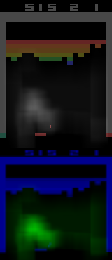
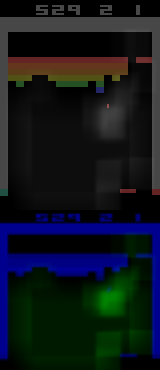
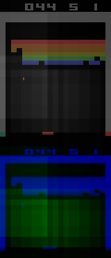
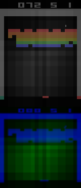
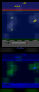
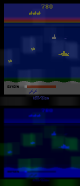
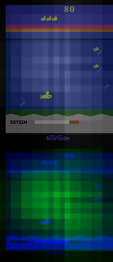
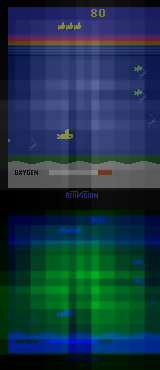
(a)	(b)	(c)	(d)	(e)	(f)	(g)	(h)

Figure 4: Game visualizations: (a-d) Breakout; (e-h) Seaquest; (a,b,e,f) Dense FLS; (c,d,g,h) Sparse FLS.

Fig. 5 shows similar visualizations on the Atari-HEAD dataset. We have also made a full gameplay video available at https://youtu.be/i41rQXKsa50.

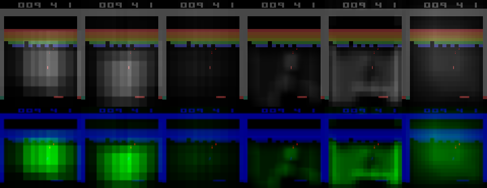
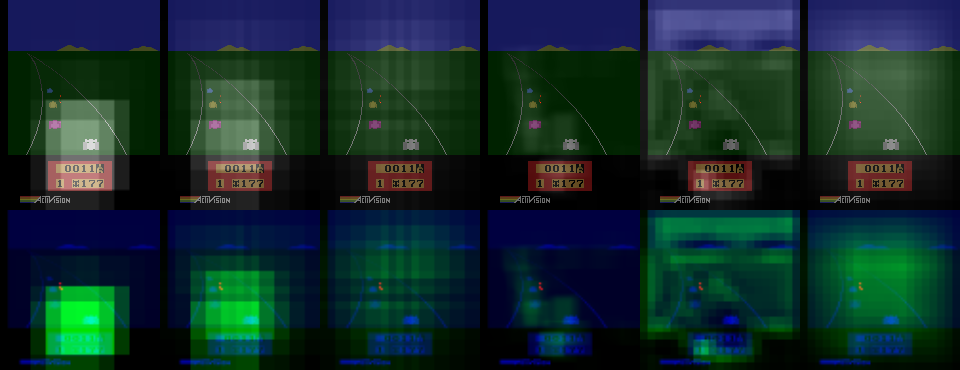
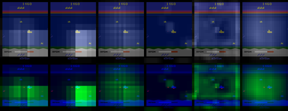
(a)	(b)	(c)
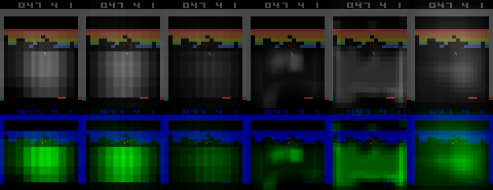
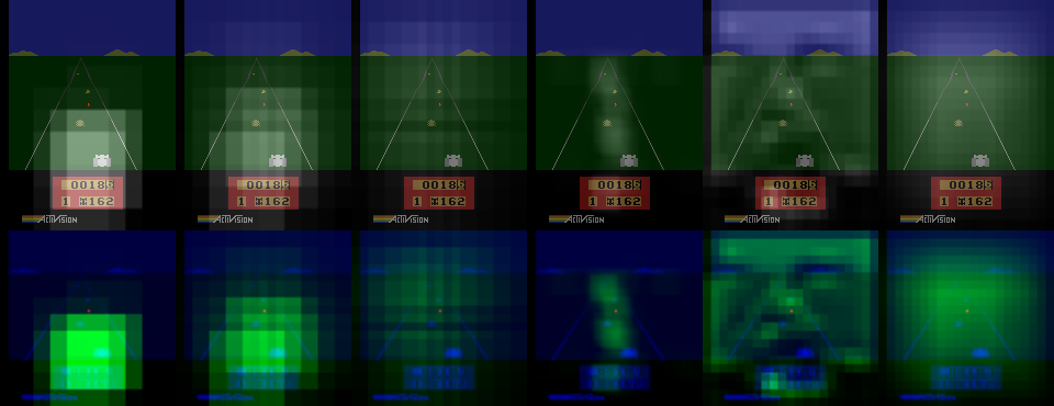
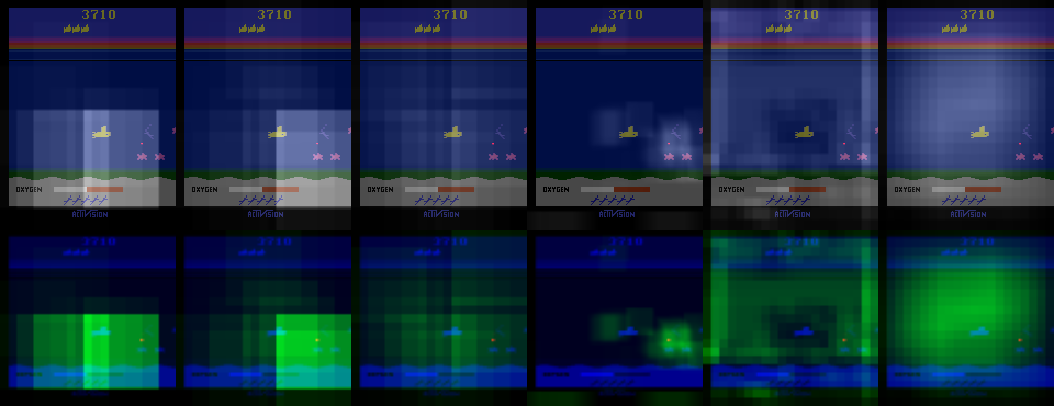
(d)	(e)	(f)

Figure 5: Atari-HEAD visualizations: (a,d) Breakout; (b,e) Enduro; (c,f) Seaquest. Each image shows the same frame with saliency maps produced by, left to right: DAQN [36], RS-PPO [42], Sparse FLS, Dense FLS, Sparse + FLS after first conv layer, Sparse + FLS after each conv layer. Human eye fixations are shown in red.

5 Conclusion

In this work, we have addressed the need for clear interpretable explanations for the behaviour of deep RL agents. We have proposed two new attention-based architectures designed to obtain saliency maps in the process of training while having competitive performance. Experiments on Atari environments show that our architectures (both Sparse and Dense) allow to get interpretable visualizations and also exhibit several other advantages: the Sparse model with sum-pooling is smaller in terms of the number of parameters, while the Dense model provides the best visualizations.

We have studied two feature extractors for deep RL playing Atari games. The Sparse FLS model achieves results very similar to the baseline but yields coarse visualizations. The Dense FLS model, to the contrary, provides crisp images but achieves lower scores. One obvious open question is how to strike the balance between the two models we present. One plays well but yields worse visualizations, the other plays worse but produces excellent pictures — can we have the best of both worlds? Our results suggest that inserting an attention module between early convolutional layers where receptive fields are small or using multiple attention modules does not improve visualizations. One possible idea for further research would be to use multiple attention modules and maintain a loss term such as KL divergence to ensure that different modules yield similar attention maps. The attention modules could also be penalized with entropy loss. A visual attention module such as FLS could also improve interpretability in contexts other than deep reinforcement learning, such as image classification; this is also an avenue for further work. In general, we believe that visualizations can be further improved with custom loss functions, which again are a subject for further research.

A visual attention module such as FLS could also improve interpretability in contexts other than reinforcement learning, such as image classification; this is also an avenue for further work. We believe that continued work in this direction may improve state of the art in deep learning interpretability even further.

6 Appendix

6.1 Performance details

Figs. 6–7 show curves for some models omitted in Fig. 3.

Figs. 8–14 show in detail performance evaluations summarized in Table 3. Each scatterplot corresponds to one model. Each circle in each scatterplot corresponds to one completed episode. The horizontal axis shows the number of steps in the episodes; the vertical axis shows attained reward. Color is proportional to density.

6.2 Breakout is censored

We pay special attention to Breakout (Fig. 8–9) because it is a popular benchmark. During experimentation, we noticed that none of the episodes attained a score greater than 864. It turned out that this was by design; the blocks could be cleared out only twice and did not respawn for the third time. This feature hampers our ability to compare agents that play the game; indeed, performance approaches 864 asymptotically, while variance remains high, making differences between models imperceptible. To work around this issue, we modified the original game so that blocks would respawn each time they are cleared and called the modified version “BreakoutInfinite”. We did so by patching the atari-py wrapper from OpenAI to overwrite the score value in the emulator RAM: as soon as the value of 864 is attained, we replace it with 432, which triggers the built-in game logic for respawning blocks. We evaluated all of our models on the modified environment in addition to the standard one. The results are shown in Table 5.

Game	Breakout	BreakoutInfinite
Nature CNN [24]	618$\pm$209	652$\pm$274 (+5.4%)
DAQN [36]	601$\pm$201	622$\pm$245 (+3.5%)
RS-PPO [42]	605$\pm$202	625$\pm$244 (+3.3%)
RS-PPO [42] w/o padding	591$\pm$199	606$\pm$234 (+2.5%)
Sparse FLS	624$\pm$211	663$\pm$283 (+6.4%)
Sparse FLS + sum-pooling	520$\pm$183	529$\pm$204 (+1.6%)
Sparse FLS + norm	598$\pm$200	621$\pm$247 (+3.8%)
Sparse FLS w/ $1\times 1$ convs	621$\pm$207	650$\pm$272 (+4.8%)
Sparse FLS w/ $\operatorname{SoftPlus}_{2}$	612$\pm$208	641$\pm$268 (+4.8%)
Sparse FLS w/o final ReLU	589$\pm$207	614$\pm$255 (+4.4%)
Sparse FLS w/o final ReLU + SP	480$\pm$158	484$\pm$172 (+0.9%)
Sparse + FLS after first conv layer	640$\pm$212	689$\pm$291 (+7.6%)
Sparse + FLS after each conv layer	633$\pm$217	681$\pm$302 (+7.7%)
Dense FLS + sum-pooling	532$\pm$173	534$\pm$182 (+0.3%)
Dense FLS w/o final ReLU + SP	503$\pm$162	506$\pm$171 (+0.6%)

Table 5: Comparison of evaluation scores for original and modified Breakout. SP denotes sum-pooling. Colors correspond to Fig. 3.

We see that, as expected, in all cases the models perform better. However, the difference is not overwhelming, and never exceeds 8%. Although we have not tested this, we hypothesize that training on “BreakoutInfinite” may improve model performance.

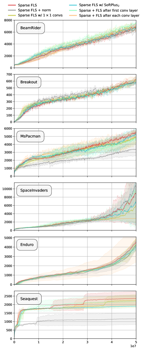
Figure 6: Reward curves for some models omitted in Fig. 3, highlighting various modifications of Sparse FLS.

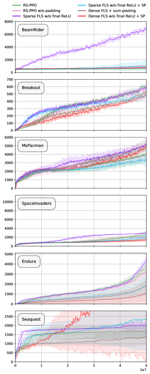
Figure 7: Reward curves for some models omitted in Fig. 3. Note that RS-PPO w/o padding performs about as well as vanilla RS-PPO, and missing ReLU before attention destroys performance (except for Dense FLS on Seaquest).

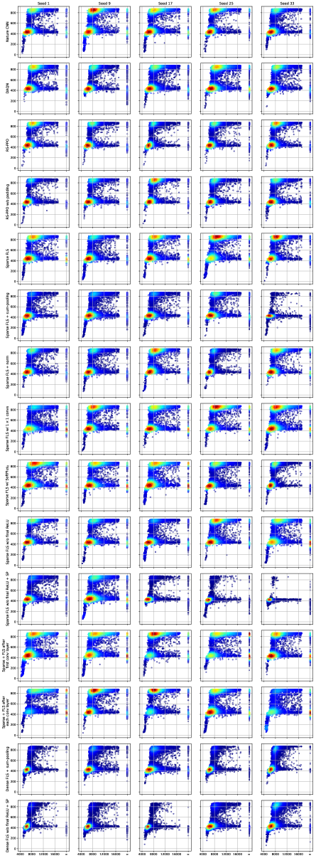
Figure 8: Breakout scatterplot.

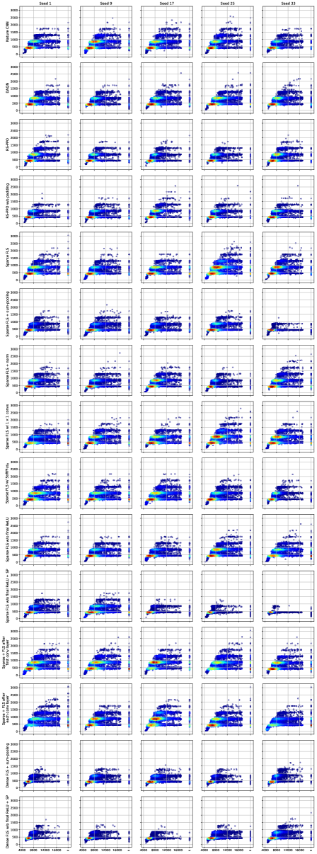
Figure 9: BreakoutInfinite scatterplot. See 6.2 for more details.

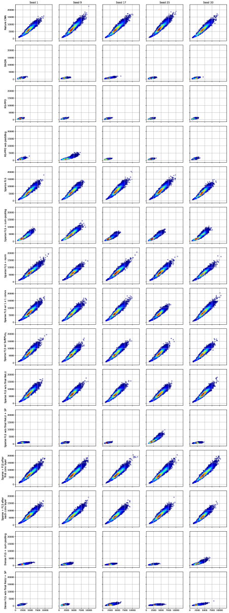
Figure 10: BeamRider scatterplot.

Figure 11: MsPacman scatterplot.

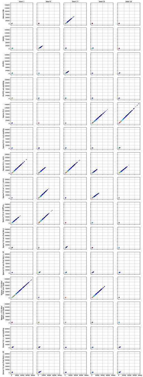
Figure 12: SpaceInvaders scatterplot.

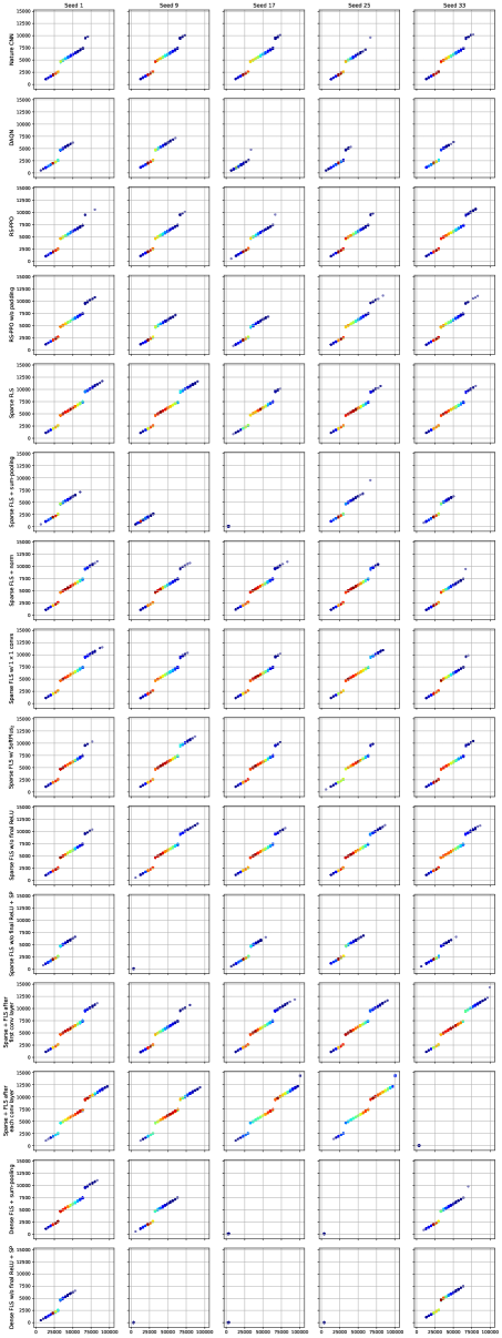
Figure 13: Enduro scatterplot.

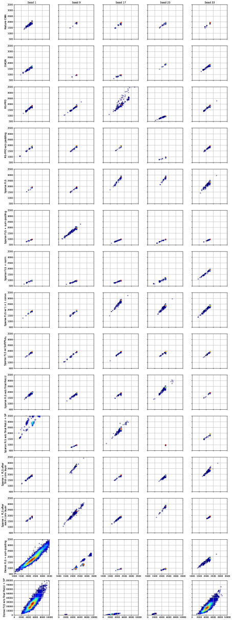
Figure 14: Seaquest scatterplot. Note the difference in scale on the vertical axis between the last model and the other ones.

References

- [1] J. Adebayo, J. Gilmer, I. Goodfellow, and B. Kim. Local explanation methods for deep neural networks lack sensitivity to parameter values. arXiv preprint arXiv:1810.03307, 2018.
- [2] K. Arulkumaran, M. P. Deisenroth, M. Brundage, and A. A. Bharath. Deep reinforcement learning: A brief survey. IEEE Signal Processing Magazine, 34(6):26–38, Nov 2017.
- [3] S. Bach, A. Binder, G. Montavon, F. Klauschen, K.-R. Müller, and W. Samek. On pixel-wise explanations for non-linear classifier decisions by layer-wise relevance propagation. PloS one, 10(7):e0130140, 2015.
- [4] D. Bahdanau, K. Cho, and Y. Bengio. Neural machine translation by jointly learning to align and translate. 2014.
- [5] M. G. Bellemare, Y. Naddaf, J. Veness, and M. Bowling. The arcade learning environment: An evaluation platform for general agents. Journal of Artificial Intelligence Research, 47:253–279, jun 2013.
- [6] A. Borji, D. N. Sihite, and L. Itti. Quantitative analysis of human-model agreement in visual saliency modeling: A comparative study. IEEE Transactions on Image Processing, 22(1):55–69, 2012.
- [7] G. Brockman, V. Cheung, L. Pettersson, J. Schneider, J. Schulman, J. Tang, and W. Zaremba. OpenAI Gym. arXiv preprint arXiv:1606.01540, 2016.
- [8] S. Chakraborty, R. Tomsett, R. Raghavendra, D. Harborne, M. Alzantot, F. Cerutti, M. Srivastava, A. Preece, S. Julier, R. M. Rao, T. D. Kelley, D. Braines, M. Sensoy, C. J. Willis, and P. Gurram. Interpretability of deep learning models: A survey of results. In 2017 IEEE SmartWorld, Ubiquitous Intelligence Computing, Advanced Trusted Computed, Scalable Computing Communications, Cloud Big Data Computing, Internet of People and Smart City Innovation (SmartWorld/SCALCOM/UIC/ATC/CBDCom/IOP/SCI), pages 1–6, Aug 2017.
- [9] Y. Chen, R. Zhu, and H. Liang. 10703 course project final report: Observe, attend and act: Attention mechanisms in DQN. page 8, 2017.
- [10] J. Choi, B.-J. Lee, and B.-T. Zhang. Multi-focus attention network for efficient deep reinforcement learning. 2017.
- [11] P. Dhariwal, C. Hesse, O. Klimov, A. Nichol, M. Plappert, A. Radford, J. Schulman, S. Sidor, Y. Wu, and P. Zhokhov. OpenAI Baselines. https://github.com/openai/baselines, 2017.
- [12] C. Dugas, Y. Bengio, F. Bélisle, C. Nadeau, and R. Garcia. Incorporating second-order functional knowledge for better option pricing. In Advances in neural information processing systems, pages 472–478, 2001.
- [13] L. Espeholt, H. Soyer, R. Munos, K. Simonyan, V. Mnih, T. Ward, Y. Doron, V. Firoiu, T. Harley, I. Dunning, et al. Impala: Scalable distributed deep-rl with importance weighted actor-learner architectures. arXiv preprint arXiv:1802.01561, 2018.
- [14] V. François-Lavet, P. Henderson, R. Islam, M. G. Bellemare, and J. Pineau. An introduction to deep reinforcement learning. CoRR, abs/1811.12560, 2018.
- [15] S. Greydanus, A. Koul, J. Dodge, and A. Fern. Visualizing and understanding atari agents. 2017.
- [16] J. Harel, C. Koch, and P. Perona. Graph-based visual saliency. In Proceedings of the 19th International Conference on Neural Information Processing Systems, NIPS’06, pages 545–552, Cambridge, MA, USA, 2006. MIT Press.
- [17] M. Hausknecht and P. Stone. Deep recurrent q-learning for partially observable MDPs. 2015.
- [18] P. Henderson, R. Islam, P. Bachman, J. Pineau, D. Precup, and D. Meger. Deep reinforcement learning that matters. In Thirty-Second AAAI Conference on Artificial Intelligence, 2018.
- [19] M. Hessel, J. Modayil, H. van Hasselt, T. Schaul, G. Ostrovski, W. Dabney, D. Horgan, B. Piot, M. G. Azar, and D. Silver. Rainbow: Combining improvements in deep reinforcement learning. In Proceedings of the Thirty-Second AAAI Conference on Artificial Intelligence, (AAAI-18), the 30th innovative Applications of Artificial Intelligence (IAAI-18), and the 8th AAAI Symposium on Educational Advances in Artificial Intelligence (EAAI-18), New Orleans, Louisiana, USA, February 2-7, 2018, pages 3215–3222, 2018.
- [20] S. Hooker, D. Erhan, P.-J. Kindermans, and B. Kim. Evaluating feature importance estimates. arXiv preprint arXiv:1806.10758, 2018.
- [21] L. Itti, C. Koch, and E. Niebur. A model of saliency-based visual attention for rapid scene analysis. IEEE Transactions on Pattern Analysis & Machine Intelligence, (11):1254–1259, 1998.
- [22] A. Manchin, E. Abbasnejad, and A. v. d. Hengel. Reinforcement learning with attention that works: A self-supervised approach. 2019.
- [23] V. Mnih, K. Kavukcuoglu, D. Silver, A. Graves, I. Antonoglou, D. Wierstra, and M. Riedmiller. Playing Atari with deep reinforcement learning. page 9, 2013.
- [24] V. Mnih, K. Kavukcuoglu, D. Silver, A. A. Rusu, J. Veness, M. G. Bellemare, A. Graves, M. Riedmiller, A. K. Fidjeland, G. Ostrovski, S. Petersen, C. Beattie, A. Sadik, I. Antonoglou, H. King, D. Kumaran, D. Wierstra, S. Legg, and D. Hassabis. Human-level control through deep reinforcement learning. 518(7540):529–533, 2015.
- [25] A. Mott, D. Zoran, M. Chrzanowski, D. Wierstra, and D. J. Rezende. Towards interpretable reinforcement learning using attention augmented agents. CoRR, abs/1906.02500, 2019.
- [26] S. Mousavi, M. Schukat, E. Howley, A. Borji, and N. Mozayani. Learning to predict where to look in interactive environments using deep recurrent q-learning. 2016.
- [27] H. Noh, A. Araujo, J. Sim, T. Weyand, and B. Han. Large-scale image retrieval with attentive deep local features. 2016.
- [28] R. J. Peters, A. Iyer, L. Itti, and C. Koch. Components of bottom-up gaze allocation in natural images. Vision research, 45(18):2397–2416, 2005.
- [29] N. Riche, M. Duvinage, M. Mancas, B. Gosselin, and T. Dutoit. Saliency and human fixations: State-of-the-art and study of comparison metrics. In Proceedings of the IEEE international conference on computer vision, pages 1153–1160, 2013.
- [30] J. Schulman, F. Wolski, P. Dhariwal, A. Radford, and O. Klimov. Proximal policy optimization algorithms. 2017.
- [31] R. R. Selvaraju, M. Cogswell, A. Das, R. Vedantam, D. Parikh, and D. Batra. Grad-cam: Visual explanations from deep networks via gradient-based localization. In Proceedings of the IEEE International Conference on Computer Vision, pages 618–626, 2017.
- [32] J. Seo, J. Choe, J. Koo, S. Jeon, B. Kim, and T. Jeon. Noise-adding methods of saliency map as series of higher order partial derivative. arXiv preprint arXiv:1806.03000, 2018.
- [33] A. Shrikumar, P. Greenside, and A. Kundaje. Learning important features through propagating activation differences. In Proceedings of the 34th International Conference on Machine Learning-Volume 70, pages 3145–3153. JMLR. org, 2017.
- [34] K. Simonyan, A. Vedaldi, and A. Zisserman. Deep Inside Convolutional Networks: Visualising Image Classification Models and Saliency Maps. arXiv e-prints, page arXiv:1312.6034, Dec 2013.
- [35] D. Smilkov, N. Thorat, B. Kim, F. Viégas, and M. Wattenberg. Smoothgrad: removing noise by adding noise. arXiv preprint arXiv:1706.03825, 2017.
- [36] I. Sorokin, A. Seleznev, M. Pavlov, A. Fedorov, and A. Ignateva. Deep attention recurrent q-network. 2015.
- [37] J. T. Springenberg, A. Dosovitskiy, T. Brox, and M. Riedmiller. Striving for simplicity: The all convolutional net. arXiv preprint arXiv:1412.6806, 2014.
- [38] M. Sundararajan, A. Taly, and Q. Yan. Axiomatic attribution for deep networks. In Proceedings of the 34th International Conference on Machine Learning-Volume 70, pages 3319–3328. JMLR. org, 2017.
- [39] R. S. Sutton and A. G. Barto. Reinforcement Learning. MIT Press, Cambridge, MA, 2nd edition, 2018.
- [40] Z. Wang, T. Schaul, M. Hessel, H. van Hasselt, M. Lanctot, and N. de Freitas. Dueling network architectures for deep reinforcement learning. 2015.
- [41] L. Weitkamp, E. van der Pol, and Z. Akata. Visual rationalizations in deep reinforcement learning for Atari games. 2019.
- [42] Z. Yang, S. Bai, L. Zhang, and P. H. S. Torr. Learn to interpret Atari agents. 2018.
- [43] L. Yuezhang, R. Zhang, and D. H. Ballard. An initial attempt of combining visual selective attention with deep reinforcement learning. 2018.
- [44] T. Zahavy, N. Ben-Zrihem, and S. Mannor. Graying the black box: Understanding DQNs. In International Conference on Machine Learning, pages 1899–1908, 2016.
- [45] R. Zhang, Z. Liu, L. Guan, L. Zhang, M. M. Hayhoe, and D. H. Ballard. Atari-HEAD: Atari human eye-tracking and demonstration dataset. CoRR, abs/1903.06754, 2019.
- [46] R. Zhang, Z. Liu, L. Zhang, J. A. Whritner, K. S. Muller, M. M. Hayhoe, and D. H. Ballard. AGIL: Learning attention from human for visuomotor tasks. In Proceedings of the European Conference on Computer Vision (ECCV), pages 663–679, 2018.