Mesh Variational Autoencoders with Edge Contraction Pooling

Abstract

3D shape analysis is an important research topic in computer vision and graphics. While existing methods have generalized image-based deep learning to meshes using graph-based convolutions, the lack of an effective pooling operation restricts the learning capability of their networks. In this paper, we propose a novel pooling operation for mesh datasets with the same connectivity but different geometry, by building a mesh hierarchy using mesh simplification. For this purpose, we develop a modified mesh simplification method to avoid generating highly irregularly sized triangles. Our pooling operation effectively encodes the correspondence between coarser and finer meshes in the hierarchy. We then present a variational auto-encoder structure with the edge contraction pooling and graph-based convolutions, to explore probability latent spaces of 3D surfaces. Our network requires far fewer parameters than the original mesh VAE and thus can handle denser models thanks to our new pooling operation and convolutional kernels. Our evaluation also shows that our method has better generalization ability and is more reliable in various applications, including shape generation, shape interpolation and shape embedding.

*Corresponding Author: gaolin@ict.ac.cn (Lin Gao)

1 Introduction

In recent years, 3D shape datasets have been increasingly available on the Internet. Consequently, data-driven 3D shape analysis has been an active research topic in computer vision and graphics. Apart from traditional data-driven works such as [8], recent works attempted to generalize deep neural networks from images to 3D shapes such as [32, 33, 19] for triangular meshes, [25] for point clouds, [37, 22] for voxel data, and so on. In this paper, we concentrate on deep neural networks for triangular meshes. Unlike images, 3D meshes have complex and irregular connectivity. Most existing works tend to keep mesh connectivity unchanged from layer to layer, thus losing the capability of increased receptive fields when pooling operations are applied.

As a generative network, the Variational Auto-Encoder (VAE) [17] has been widely used in various kinds of generation tasks, including generation, interpolation and exploration on triangular meshes [33]. The original MeshVAE [33] uses a fully connected network that requires a huge number of parameters and its generalization ability is often weak. Although the fully connected layers allow the changes of mesh connectivity, due to irregular changes, they cannot be followed by convolutional operations. Litany et al. [19] use the VAE structure with graph convolutions, aiming to deal with model completion. Gao et al. [11] include a spatial convolutional mesh VAE in their pipeline. However, these two kinds of convolution operations cannot change the connectivity of the mesh. The work [27] introduces sampling operations in convolutional neural networks (CNNs) on meshes, but their sampling strategy does not aggregate all the local neighborhood information when reducing the number of vertices. Therefore, in order to deal with denser models and enhance the generalization ability of the network, it is necessary to design a pooling operation for meshes similar to the pooling for images to reduce the number of network parameters. Moreover, it is desired that the defined pooling operation can support further convolutions and allow recovery of the original resolution through a relevant de-pooling operation.

In this paper we propose a VAE architecture with newly defined pooling operations. Our method uses mesh simplification to form a mesh hierarchy with different levels of details, and achieves effective pooling by keeping track of the mapping between coarser and finer meshes. To avoid generating highly irregular triangles during mesh simplification, we introduce a modified mesh simplification approach based on the classical mesh simplification algorithm [12]. The input to our network is a vertex-based deformation feature representation [10], which unlike 3D coordinates, encodes deformations using deformation gradients defined on vertices. Our framework use a collection of 3D shapes with the same connectivity to train the network. Meshes with consistent connectivity have been commonly used for various applications such as data-driven deformation [31], deformation transfer [11, 2], human shape generation [33] and shape completion [19]. Such meshes can be easily obtained through consistent remeshing. Also, we adopt graph convolutions [7] in our network. In all, our network follows a VAE architecture where pooling operations and graph convolutions are applied. As we will show later, our network not only has better generalization capabilities but also can handle much higher resolution meshes, benefiting various applications, such as shape generation, interpolation and embedding.

2 Related Work

Deep Learning for 3D Shapes. Deep learning on 3D shapes has received increasing attention. From the Euclidean domain, Boscaini et al. [3, 4] generalize CNNs to the non-Euclidean domain, which is useful for 3D shape analysis such as establishing correspondences. Bronstein et al. [6] give an overview of utilizing CNNs on non-Euclidean domains, including graphs and meshes. Masci et al. [21] proposed the first mesh convolutional operations by applying filters to local patches represented in geodesic polar coordinates. Sinha et al. [29] convert 3D shapes to geometry images to obtain a Euclidean parameterization, on which standard CNNs can be applied. Maron et al. [20] parameterize a surface to a planar flat-torus to define a natural convolution operator for CNNs on surfaces. Wang et al. [35, 36] proposed octree-based convolutions for 3D shape analysis. Unlike local patches, geometry images, planar flat-torus, or octree structure, our work performs convolutional operations using vertex features [10] as inputs.

To analyze meshes with the same connectivity but different geometry, the work [33] first introduced the VAE architecture to 3D mesh data, and demonstrates its usefulness using various applications. Tan et al. [32] use a convolutional auto-encoder to extract localized deformation components from mesh datasets with large-scale deformations. Gao et al. [11] proposed a network which combines convolutional mesh VAE with CycleGAN [39] for automatic unpaired shape deformation transfer. The works of [32, 11] apply convolutional operations to meshes in the spatial domain, while the works of [7, 13] extend CNNs to irregular graphs by construction in the spectral domain, and show superior performance when compared with spatial convolutions. Following  [7, 38], our work also performs convolutional operations in the spectral domain.

While pooling operations have been widely used in the deep networks for image processing, existing mesh-based VAE methods either do not support pooling [33, 11], or use a simple sampling process [27], which is not able to aggregate all the local neighborhood information. In fact, the sampling approach in [27], while being also based on a simplification algorithm, directly drops the vertices, and uses the barycentric coordinates in a triangle to recover the lost vertices by interpolation. In contrast, our pooling operations can aggregate local information by recording the simplification procedure, and support direct reverse of the pooling operation to effectively achieve a de-pooling operation.

Uniform Sampling or Pooling Methods. Based on point cloud, Pointnet++ [26] has proposed a uniform sampling method for point cloud based neural networks. Using the same idea, TextureNet [14] also conducts uniform sampling on the vertices of mesh. This kind of sampling method destroys the connection between vertices, turning mesh data into point cloud and cannot support further graph convolutions. Simplification methods can build mesh hierarchy, so can help us build mesh pooling operation. However, most simplification methods, such as [12], are shape-preserving, not uniform. Remeshing operation, such as [5], can build uniform simplified meshes, but loss the correspondence between hierarchies. We, therefore, modify the classical simplification [12] to simplify mesh more uniform and record the correspondences between coarse mesh and dense mesh for newly defined mesh pooling and de-pooling operations.

Deforming Mesh Representations and Applications. In order to better represent 3D meshes, a straightforward approach is to use vertex coordinates of a 3D shape. However, vertex coordinates are neither translation invariant nor rotation invariant, making it difficult to learn large-scale deformation. We instead use a recent 3D shape deformation representation [10], which compared with another widely used representation [9], has the benefit of recording deformations at vertices, making graph convolutions and pooling operations easier to achieve.

Shape generation and interpolation are common applications on mesh data. Utilizing the VAE structure, MeshVAE [33] generates more deformable mesh shapes, and the method in [27] generates 3D faces with vivid expressions from a latent space. In fact, these VAE-based methods [33, 27, 19] can also be used for the task of shape interpolation. Shape interpolation is a well researched topic. Existing mesh interpolation methods can be largely categorized into geometry-based methods (e.g. [15]) and data-driven methods (e.g. [8]). The latter exploits the information hidden in the shape dataset, and thus such approaches can produce more reasonable and reliable interpolation results. It has been shown that meshVAE [33] achieves better results than existing data-driven methods [8]. However, [33] cannot deal with the shapes that contain too many vertices (e.g. the elephant model from [31]), which restricts the resolution of generated mesh shapes. Although the method in [27] performs well on face shapes, its reconstruction results on human body [34] are not satisfactory. Our work is also based on the VAE architecture, and therefore can naturally be used for shape generation and shape interpolation. Our framework improves over MeshVAE, and has better generalization ability, as we will demonstrate later.

Figure 1: Our network architecture. $\epsilon$ is a random variable with a Gaussian distribution with 0 mean and unit variance.

3 Feature Representation

To better represent shapes used in our network, as previously discussed, we utilize a recent deformation representation [10]. We assume that shapes in the dataset have the same mesh connectivity. This assumption is satisfied by many deformable object datasets [1, 34, 31], and the same connectivity can be achieved with consistent remeshing. Let $N$ be the number of shapes in the dataset, and the $m^{\rm th}$ shape is represented as $S_{m}$. $\mathbf{p}_{m,i}\in\mathbb{R}^{3}$ is the $i^{\rm th}$ vertex on the $m^{\rm th}$ model. The deformation gradient $\mathbf{T}\in\mathbb{R}^{3\times 3}$ is a local affine transform that describes local deformation around a vertex. Using polar decomposition, $\mathbf{T}_{m,i}=\mathbf{R}_{m,i}\mathbf{S}_{m,i}$, that is, the deformation gradient $\mathbf{T}_{m,i}$ can be decomposed into a rotation matrix $\mathbf{R}_{m,i}$ and a scale/shear matrix $\mathbf{S}_{m,i}$. By collecting non-trivial entries in the rotation and scale/shear components, the deformation around the $i^{\rm th}$ vertex of the $m^{\rm th}$ shape can be represented as a vector $q_{m,i}\in\mathbb{R}^{9}$. Following [33], We further apply a linear scaling to map each element of $q_{m,i}$ to $[-0.95,0.95]$ to allow $tanh$ to be used as an activation function.

4 Our Framework

In this section we introduce the basic operations and network architecture used in our framework. We first describe our modified mesh simplification algorithm, which will be used to build mesh hierarchy for our pooling operations. Then the graph convolutional operation will be introduced. Finally we will summarize our network structure.

4.1 Mesh Simplification

Figure 2: Comparison of the mesh simplification algorithm [12] and our modified version. (a) the original mesh with 12,500 vertices, (b) a result of [12] with 6,251 vertices, and (c) our result with 6,250 vertices.

We use mesh simplification to help build reliable pooling operations. For this purpose, mesh simplification not only creates a mesh hierarchy with different levels of details, but also ensures the correspondences between coarser and finer meshes. Our simplification process is based on the classical method [12], which performs repeated edge contraction in an order based on a metric measuring shape changes. However, the original approach cannot guarantee that the simplified mesh contains evenly distributed triangles. To achieve more effective pooling, each vertex in the coarser mesh should correspond to a similarly sized region.

Our observation is that the edge length is an important indicator for this process. To avoid contracting long edges, we incorporate the edge length as one of the criteria to order pairs of points to be simplified. The original work defines the error at vertex $\mathbf{v}=[v_{x},v_{y},v_{z},1]^{\mathrm{T}}$ to be a quadratic form $\mathbf{v}^{\mathrm{T}}\mathbf{Q}\mathbf{v}$, where $\mathbf{Q}$ is the sum of the fundamental error quadrics introduced in [12]. For a given edge contraction $(\mathbf{v}_{1},\mathbf{v}_{2})\rightarrow\bar{\mathbf{v}}$, they simply choose to use $\bar{\mathbf{Q}}=\mathbf{Q}_{1}+\mathbf{Q}_{2}$ to be the new matrix which approximates the error at $\bar{\mathbf{v}}$. So the error at $\bar{\mathbf{v}}$ will be $\bar{\mathbf{v}}^{\mathrm{T}}\bar{\mathbf{Q}}\bar{\mathbf{v}}$. We propose to add the new edge length to the original simplification error metric. Specifically, given an edge $(\mathbf{v}_{i},\mathbf{v}_{j})$ to be contracted to a new vertex $\bar{\mathbf{v}}_{k}$, the total error is defined as:

$$E =\bar{\mathbf{v}}_{k}^{\mathrm{T}}\bar{\mathbf{Q}}_{k}\bar{\mathbf{v}}_{k}$$ (1)

$$+\lambda\max\{L_{km},L_{kn}|m\in\mathcal{N}_{i},n\in\mathcal{N}_{j},m\neq j,n\neq i\},$$

where $L_{km}$ (resp. $L_{kn}$) is the new edge length between vertex $k$ and vertex $m$ (resp. vertex $n$). $\mathcal{N}_{i}$ (resp. $\mathcal{N}_{j}$) is the set of neighboring vertices of vertex $i$ (resp. vertex $j$), and $\lambda$ is a weight. Note that we only penalize the maximum edge length around newly created vertices $\bar{\mathbf{v}}_{k}$ to effectively avoid triangles with too long edges. In our experiments, we contract half of the vertices between adjacent levels of details to support effective pooling. A representative simplification example is shown in Fig. 2, which clearly shows the effect of our modified simplification algorithm. The advantage of our modified simplification algorithm over the original one on pooling and thus shape reconstruction will be discussed in Section 5.1.

Figure 3: We use a simplification algorithm to introduce our pooling operation on meshes. The red vertices are simplified to the green vertex by edge contraction and the features of the red vertices are averaged to give the feature of the green vertex.

4.2 Pooling and De-pooling

Mesh simplification is achieved by repeated edge contraction, i.e., contracting two adjacent vertices to a new vertex. We exploit this process to define our pooling operation, in a way similar to image-based pooling. We use average pooling for our framework (and alternative pooling operations can be similarly defined). As illustrated in Fig. 3, following an edge contraction step, we define the feature of a new vertex as the average feature of the contracted vertices. This ensures that the pooling operation effectively operates at relevant simplified regions. This process has some advantages: It preserves a correct topology to support multiple levels of convolutions/pooling, and makes the receptive field well defined.

Since our network has a decoder structure, we also need to properly define a de-pooling operation. We similarly take advantage of simplification relationships, and define de-pooling as the inverse operation: the features of the vertices on the simplified mesh are equally assigned to the corresponding contracted vertices on the dense mesh.

4.3 Graph Convolution

To form a complete neural network architecture, we adopt the spectral graph convolutions introduced in [7]. Let $\mathbf{x}$ be the input and $\mathbf{y}$ be the output of a convolution operation. $\mathbf{x}$ and $\mathbf{y}$ are matrices where each row corresponds to a vertex and each column corresponds to a feature dimension. Let $\mathbf{L}$ denote the normalized graph Laplacian. The spectral graph convolution used in our network is then defined as

$$\mathbf{y}=g_{\theta}(\mathbf{L})\mathbf{x}=\sum_{h=0}^{H-1}{\theta_{h}\mathbf{T}_{h}(\tilde{\mathbf{L}})\mathbf{x}},$$ (2)

where $\tilde{\mathbf{L}}=2\mathbf{L}/\lambda_{max}-\mathbf{I}$, $\theta\in\mathbb{R}^{H}$ is polynomial coefficients, and $\mathbf{T}_{h}(\tilde{\mathbf{L}})\in\mathbb{R}^{V\times V}$ is the Chebyshev polynomial of order $h$ evaluated at $\tilde{\mathbf{L}}$.

4.4 Network Structure

As illustrated in Fig. 1, our overall network is built on our average pooling operation and convolutional operation, with a variational auto-encoder structure. The input to the encoder is the preprocessed features which are shaped as $X\in\mathbb{R}^{V\times 9}$, where $V$ is the number of vertices and 9 is the dimension of the deformation representation.

Unlike the original mesh VAE [33], which uses fully connected layers, our approach benefits from graph convolutions and especially, the newly defined pooling operations to massively reduce the number of parameters. The introduction of the pooling operations also improves the generalizability of the network.

Our network takes the preprocessed vertex features defined in [10] as input, which then go through two graph convolutional layers, followed by one pooling layer and another graph convolutional layer. In order to avoid overfitting, the last convolutional layer does not use any nonlinear activation function. The output of the last convolutional layer is mapped to a mean vector and a deviation vector by two different fully-connected layers. The mean vector does not have an activation function, and the deviation vector uses sigmoid as the activation function.

To reconstruct the shape representation from the latent vector, the decoder is used, which basically mirrors the encoder steps. For the decoder convolutional layers, we use the transposed weights of the corresponding layers in the encoder, with all layers using the $tanh$ output activation function. Corresponding to the pooling operation, the de-pooling operation as described in Section 4.2 maps features in a coarser mesh to a finer mesh. The output of the whole network is $\hat{X}\in\mathbb{R}^{V\times 9}$, which has the identical dimension as the input, and can be rescaled back to the deformation representation and used for reconstructing the deformed shape.

In order to train the model to fit the large dimension of mesh features, we use the mean squared error (MSE) as the reconstruction loss. Combined with the KL-divergence [18], the total loss function for the model is defined as

$$L=\frac{1}{2M}\sum_{i=1}^{M}{\|X^{i}-\hat{X}^{i}\|^{2}_{F}}+\alpha D_{KL}(q(z|X)\|p(z)),$$ (3)

where $X^{i}$ and $\hat{X}^{i}$ represent the preprocessed features of the $i^{\rm th}$ model and the output of the network. $\|\cdot\|_{F}$ is the Frobenius norm of matrix, $M$ is the number of shapes in the dataset, $\alpha$ is a parameter to adjust the priority between the reconstruction loss and KL-divergence. $z$ is the latent vector, $p(z)$ is the prior probability, $q(z|X)$ is the posterior probability, and $D_{KL}$ is the KL-divergence.

4.5 Conditional VAE

When the VAE is used for shape generation, it is often preferred to allow the selection of shape types to be generated, especially for datasets containing shapes from different categories (such as men and women, thin and fat, see [24] for more examples). To achieve this, we refer to [30] and add labels to the input and the latent vectors to extend our framework. In this case, our loss function is changed to

$$L_{c}=\frac{1}{2M}\sum_{i=1}^{M}{\|X_{c}^{i}-\hat{X}^{i}\|^{2}_{F}}+\alpha D_{KL}(q(z|X,c)\|p(z|c)),$$ (4)

where $\hat{X}$ is the output of the conditional VAE, and $p(z|c)$ and $q(z|X,c)$ are conditional prior and posterior probabilities, respectively.

4.6 Implementation Details

In our experiments, we contract half of the vertices with $\lambda=0.001$ in Eq. 1 and set the hyper-parameter $H=3$ in graph convolutions, $\alpha=0.3$ in the total loss function. The latent space dimension is 128 for all our experiments. We also use $L_{2}$ regularization on the network weights to avoid over-fitting. We use Adam optimizer [16] with the learning rate set to $0.001$.

Dataset	Only	Only	[12]	Uniform	Graph	Mesh	Our
	Spatial Conv.	Spectral Conv.		Simp.	Pooling	Sampling	Method
SCAPE	0.1086	0.0825	0.0898	0.0813	0.0824	0.0831	0.0763
Swing	0.0359	0.0282	0.0284	0.0281	0.0292	0.0298	0.0268
Fat	0.0362	0.0267	0.0285	0.0305	0.0253	0.0289	0.0249
Hand	0.0300	0.0284	0.0271	0.0280	0.0306	0.0278	0.0260

Table 1: Comparison of RMS reconstruction errors for unseen data using our network with pooling, without pooling, with different convolutional operators, with original simplification [12]-based pooling, with uniform simplification-based pooling (remeshing [5]), with graph pooling [28] and with mesh sampling [27]. Note that ’Only Spectral Conv.’ also means ’No Pooling’.

Dataset	‘CPCPC’	‘CCPCCPC’	Our Network
SCAPE	0.0942	0.0863	0.0763

Table 2: Comparison of different network structures. ‘C’ and ‘P’ refer to a graph convolutional layer and a pooling layer respectively.

Dataset	#. Vertices	Tan	Gao	Ranjan	Ours
		2018	2018	2018
SCAPE	12500	-	0.1086	0.1095	0.0763
Swing	9971	-	0.0359	0.0557	0.0268
Fat	6890	0.0308	0.0362	0.0324	0.0249
Hand	3573	0.0362	0.0300	0.0632	0.0260
Face	11849	-	1.0619	1.1479	0.7257
Horse	8431	-	0.0128	0.0510	0.0119
Camel	11063	-	0.0134	0.0265	0.0115

Table 3: Comparison of RMS reconstruction errors for unseen data using different auto-encoder frameworks proposed by Tan et al.  [33], Gao et al. [11], and Ranjan et al. [27]. ‘-’ means the corresponding method runs out of memory (largely due to the use of fully connected networks).

Dataset	#. Vertices	Tan et al. 2018	Ours
Fat	6890	129,745,920	7,941,042
Hand	3573	68,610,048	4,118,706

Table 4: Comparison of parameters number with [33]. It can be seen that our network require far fewer parameters than [33].

5 Experiments

5.1 Framework Evaluation

To compare different network structures and settings, we use several shape deformation datasets, including SCAPE dataset [1], Swing dataset [34], Face dataset [23], Horse and Camel dataset [31], Fat (ID:50002) from the MPI DYNA dataset [24], and Hand dataset. For each dataset, it is randomly split into halves for training and testing. We test the capability of the network to generate unseen shapes, and report the average RMS (root mean squared) errors.

Effect of Pooling. In Table 1 (Column 3 and 8) we compare the RMS errors of reconstructing unseen shapes with and without pooling. The RMS error is lower by an average of $8.36\%$ with pooling. The results show the benefit of our pooling and de-pooling operations.

Comparison with Spatial Convolutions. We compare spectral graph convolutions with alternative spatial convolutions, both with a similar network architecture as shown in Fig. 1. The comparison results are shown in Table 1 (Column 2 and 3). One can easily find that spectral graph convolutions give better results.

Comparisons with Other Pooling or Sampling Methods. To demonstrate the benefit of our simplification-based pooling operation, we compare our pooling with with the original algorithm [12] for pooling, the existing graph pooling method [28], and the mesh sampling operation introduced in [27]. What’s more, we show comparisons to a representative uniform simplification method based on remeshing [5]. This method is able to distribute vertices uniformly but loses geometry details. In contrast, our method aims for a uniform, and also shape-preserving simplification, which leads to better results. The results are shown in Table 1. The RMS error of our pooling for unseen data is lower by an average of $9.17\%$ compared to [12]-based pooling, $8.06\%$ compared to graph pooling [28], and $9.64\%$ compared to mesh sampling [27], which shows our modified simplification algorithm is more effective in term of pooling and our pooling is superior on multiple datasets, leading to better generalization ability.

Figure 4: Qualitative comparison of reconstruction results for unseen data with  [11]. Reconstruction errors are color-coded. It can be seen that our method leads to more accurate reconstructions.

Figure 5: Qualitative comparison of reconstruction results for unseen data with  [27]. Our method leads to significantly lower reconstruction errors.

Figure 6: Qualitative comparison of reconstruction results with  [27]. The method of [27] suffers from easily noticeable artifacts.

Figure 7: Randomly generated new shapes using our framework, along with their nearest neighbors (NN) in the original datasets.

Figure 8: Conditional random generation of new shapes using our framework.

Alternative Network Structures. In addition to the architecture shown in Fig. 1, we also consider alternative architectures, including adding more convolutional and pooling layers (see Table 2). It can be seen that our chosen architecture has better performance than alternative architectures. This shows that our architecture is flexible enough to learn from the data but not overly complicated which might lead to overfitting.

Comparison with State-of-the-Art. In Table 3, we compare our method with the state-of-the-art mesh-based auto-encoder architectures [11, 27, 33] in terms of RMS errors of reconstructing unseen shapes. Thanks to spectral graph convolutions and our pooling, our method consistently reduces the reconstruction errors of unseen data, showing superior generalizability. For example, compared with [11], which uses the same per-vertex features as ours, our network achieves $29\%$ and $32\%$ lower average RMS reconstruction errors on the SCAPE and Face datasets. What’s more, we show the qualitative reconstruction comparison with [11] and [27] in Fig. 4, 5 and 6. These figures show that our method leads to more accurate reconstruction results than [11, 27]. In Table 4, we present two comparisons to illustrate that our network requires far fewer parameters than the original MeshVAE.

Figure 9: Comparison of mesh interpolation results with [33]. The models in the leftmost and rightmost columns are the input models to be interpolated. 1st row: the results of [33], and 2nd row: our results.

5.2 Generation of Novel Models

Once our network is trained, we can use the latent space and decoder to generate new shapes. We use the standard normal distribution $z\sim N(0,I)$ as the input to the trained decoder. It can be seen from Fig. 7 that our network is capable of generating reasonable new shapes. To prove that the generated shapes do not exist in the model dataset, we find the nearest shapes based on the average per-vertex Euclidean distance in the original datasets for visual comparison. It can be seen that the generated shapes are indeed new and different from any existing shape in the datasets. To show our conditional random generation ability, we train the network on the DYNA dataset from [24]. We use BMI+gender and motion as the condition to train the network. As shown in Fig. 8, our method is able to randomly generate models that are conditioned on the body shape ‘50007’ – a male model with BMI 39.0 and conditioned on the action with the label ‘One Leg Jump’ including lifting the leg.

Figure 10: Comparison of mesh interpolation results with [8] (1st row). The models in the leftmost and rightmost columns are the input models to be interpolated.

Figure 11: Comparison of mesh interpolation results with [19]. First row is the result of [19], and second row is our result.

Figure 12: Interpolation comparison between Mesh VAE [33] and our method. The original elephant model [31] has 42,321 vertices, which cannot be handled by Mesh VAE due to memory restriction and therefore a simplified mesh with 5,394 vertices is used instead. Our method operates on the original mesh model and produces results with more details.

5.3 Mesh Interpolation

Our method can also be used for shape interpolation. This is because VAE compresses complex 3D models into a low-dimensional latent vector. We test the capability of our framework to interpolate two different shapes in the original dataset. First, we generate the mean outputs of the probabilistic encoder for two shapes. Then, we linearly interpolate between the two latent vectors and generate a sequence of latent vectors for the probabilistic decoder. Finally, we use the outputs of the probabilistic decoder to reconstruct a 3D deformation sequence. We compare our method on the SCAPE dataset [1] with Mesh VAE [33], and a state-of-the-art data-driven deformation method [8], as shown in Figures 9 and 10 respectively. We can see that Mesh VAE [33] produces interpolation results with obvious artifacts. The results by the data-driven method of [8] tend to follow the movement sequences from the original dataset which has similar start and end states, leading to redundant motions such as the swing of right arm. In contrast, our interpolation results give more reasonable motion sequences. In Fig. 11, we show a comparison with the method of [19], which leads to artifacts especially in the synthesized human hands. We show more interpolation results in Fig. 13, including sequences between newly generated models and models beyond human bodies.

To show the ability of our network for processing denser meshes, we compare our network with Mesh VAE [33]. Mesh VAE can handle much smaller-resolution meshes due to the high memory demands of their fully connected network. This is not a problem with our method thanks to the convolution kernels and pooling operations. Therefore our method can recover superior details for interpolation, reconstruction and random generation. A comparison example for interpolation is shown in Fig. 12.

Figure 13: More interpolation results. (a)(b) more diverse shapes other than human bodies. (c) results interpolated between newly generated shapes.

5.4 Embedding

Our method can compress 3D shapes into low dimensional vectors for visualization. To better visualize the embedding, we calculate the two largest variances of the latent vector as the horizontal and vertical coordinates of the model in the 2D embedding graph. We utilize this capability to embed shapes in a low-dimensional space. Our method divides all the models according to their shapes, while allowing models of similar poses to stay in close places. We use a representative motion sequences of different deformation types, namely a horse motion sequence from [31]. The Horse dataset [31] contains a motion sequence of a galloping horse, which forms a cyclic sequence. We can conclude from the embedding result shown in Fig. 14, that a circle is formed that matches the original sequence, which shows that our network has good embedding ability. We also show comparison with t-SNE and PCA in Fig. 15. Our result presents as two circles, while t-SNE and PCA cannot reveal the intrinsic information of the data.

Figure 14: 2D embedding of Horse dataset [31]. The result presented as a circle matching the cyclic motion sequence.

(a) Our

(b) t-SNE

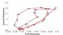
(c) PCA

Figure 15: Embedding comparisons with t-SNE and PCA.

6 Conclusions

In this paper we introduced a newly defined pooling operation based on a modified mesh simplification algorithm and integrated it into a mesh variational auto-encoder architecture, which uses per-vertex feature representations as inputs, and utilizes graph convolutions. Through extensive experiments we demonstrated that our generative model has better generalization ability. Compared to the original Mesh VAE, our method can generate high quality deformable models with richer details. Our experiments also show that our method outperforms the state-of-the-art methods in various applications including shape generation and shape interpolation. One of the limitations of our method is that it can process only homogeneous meshes. As a future work, it is desirable to develop a framework capable of handling shapes with different topology as input.

References

- [1] D. Anguelov, P. Srinivasan, D. Koller, S. Thrun, J. Rodgers, and J. Davis. Scape: shape completion and animation of people. ACM transactions on graphics, 24(3):408–416, 2005.
- [2] I. Baran, D. Vlasic, E. Grinspun, and J. Popović. Semantic deformation transfer. TOG, 28(3):36:1–36:6, July 2009.
- [3] D. Boscaini, J. Masci, E. Rodolà, and M. Bronstein. Learning shape correspondence with anisotropic convolutional neural networks. In NIPS, pages 3189–3197, 2016.
- [4] D. Boscaini, J. Masci, E. Rodolà, M. M. Bronstein, and D. Cremers. Anisotropic diffusion descriptors. Computer Graphics Forum, 35(2):431–441, 2016.
- [5] M. Botsch and L. Kobbelt. A remeshing approach to multiresolution modeling. In SGP, pages 185–192, 2004.
- [6] M. M. Bronstein, J. Bruna, Y. LeCun, A. Szlam, and P. Vandergheynst. Geometric deep learning: going beyond euclidean data. IEEE Signal Processing Magazine, 34(4):18–42, 2017.
- [7] M. Defferrard, X. Bresson, and P. Vandergheynst. Convolutional neural networks on graphs with fast localized spectral filtering. In Advances in NIPS, pages 3844–3852, 2016.
- [8] L. Gao, S.-Y. Chen, Y.-K. Lai, and S. Xia. Data-driven shape interpolation and morphing editing. Computer Graphics Forum, 36(8):19–31, 2017.
- [9] L. Gao, Y.-K. Lai, D. Liang, S.-Y. Chen, and S. Xia. Efficient and flexible deformation representation for data-driven surface modeling. ACM Transactions on Graphics, 35(5):158:1–158:17, 2016.
- [10] L. Gao, Y.-K. Lai, J. Yang, L.-X. Zhang, L. Kobbelt, and S. Xia. Sparse data driven mesh deformation. arXiv preprint arXiv:1709.01250, 2017.
- [11] L. Gao, J. Yang, Y.-L. Qiao, Y. Lai, P. Rosin, W. Xu, and S. Xia. Automatic unpaired shape deformation transfer. ACM Transactions on Graphics, 37(6):1–15, 2018.
- [12] M. Garland and P. S. Heckbert. Surface simplification using quadric error metrics. In Siggraph, pages 209–216, 1997.
- [13] M. Henaff, J. Bruna, and Y. LeCun. Deep convolutional networks on graph-structured data. arXiv preprint arXiv:1506.05163, 2015.
- [14] J. Huang, H. Zhang, L. Yi, T. Funkhouser, M. Niessner, and L. J. Guibas. Texturenet: Consistent local parametrizations for learning from high-resolution signals on meshes. In The IEEE Conference on Computer Vision and Pattern Recognition (CVPR), June 2019.
- [15] P. Huber, R. Perl, and M. Rumpf. Smooth interpolation of key frames in a riemannian shell space. Computer Aided Geometric Design, 52:313–328, 2017.
- [16] D. P. Kingma and J. Ba. Adam: A method for stochastic optimization. arXiv preprint arXiv:1412.6980, 2014.
- [17] D. P. Kingma and M. Welling. Auto-encoding variational bayes. arXiv preprint arXiv:1312.6114, 2013.
- [18] S. Kullback and R. A. Leibler. On information and sufficiency. The annals of mathematical statistics, 22(1):79–86, 1951.
- [19] O. Litany, A. Bronstein, M. Bronstein, and A. Makadia. Deformable shape completion with graph convolutional autoencoders. In The IEEE Conference on Computer Vision and Pattern Recognition (CVPR), June 2018.
- [20] H. Maron, M. Galun, N. Aigerman, M. Trope, N. Dym, E. Yumer, V. G. Kim, and Y. Lipman. Convolutional neural networks on surfaces via seamless toric covers. ACM Transactions on Graphics, 36(4):71, 2017.
- [21] J. Masci, D. Boscaini, M. Bronstein, and P. Vandergheynst. Geodesic convolutional neural networks on riemannian manifolds. In ICCV workshops, pages 37–45, 2015.
- [22] D. Maturana and S. Scherer. VoxNet: A 3D Convolutional Neural Network for Real-Time Object Recognition. In IROS, 2015.
- [23] T. Neumann, K. Varanasi, S. Wenger, M. Wacker, M. Magnor, and C. Theobalt. Sparse localized deformation components. ACM Transactions on Graphics (TOG), 32(6):179, 2013.
- [24] G. Pons-Moll, J. Romero, N. Mahmood, and M. J. Black. Dyna: A model of dynamic human shape in motion. ACM Transactions on Graphics, 34(4):120, 2015.
- [25] C. R. Qi, H. Su, K. Mo, and L. J. Guibas. Pointnet: Deep learning on point sets for 3d classification and segmentation. arXiv preprint arXiv:1612.00593, 2016.
- [26] C. R. Qi, L. Yi, H. Su, and L. J. Guibas. Pointnet++: Deep hierarchical feature learning on point sets in a metric space. In Advances in Neural Information Processing Systems, pages 5099–5108. Curran Associates, Inc., 2017.
- [27] A. Ranjan, T. Bolkart, S. Sanyal, and M. J. Black. Generating 3D faces using convolutional mesh autoencoders. In European Conference on Computer Vision (ECCV), pages 725–741. Springer International Publishing, 2018.
- [28] Y. Shen, C. Feng, Y. Yang, and D. Tian. Mining point cloud local structures by kernel correlation and graph pooling. In CVPR, volume 4, 2018.
- [29] A. Sinha, J. Bai, and K. Ramani. Deep learning 3d shape surfaces using geometry images. In ECCV, pages 223–240, 2016.
- [30] K. Sohn, H. Lee, and X. Yan. Learning structured output representation using deep conditional generative models. In Advances in NIPS, pages 3483–3491, 2015.
- [31] R. W. Sumner and J. Popović. Deformation transfer for triangle meshes. ACM Transactions on Graphics, 23(3):399–405, 2004.
- [32] Q. Tan, L. Gao, Y. Lai, J. Yang, and S. Xia. Mesh-based autoencoders for localized deformation component analysis. In AAAI, 2018.
- [33] Q. Tan, L. Gao, Y.-K. Lai, and S. Xia. Variational autoencoders for deforming 3d mesh models. In CVPR, June 2018.
- [34] D. Vlasic, I. Baran, W. Matusik, and J. Popović. Articulated mesh animation from multi-view silhouettes. ACM Transactions on Graphics, 27(3):97, 2008.
- [35] P.-S. Wang, Y. Liu, Y.-X. Guo, C.-Y. Sun, and X. Tong. O-CNN: Octree-based Convolutional Neural Networks for 3D Shape Analysis. ACM Transactions on Graphics (SIGGRAPH), 36(4), 2017.
- [36] P.-S. Wang, Y. Liu, Y.-X. Guo, C.-Y. Sun, and X. Tong. Adaptive O-CNN: A Patch-based Deep Representation of 3D Shapes. ACM Transactions on Graphics (SIGGRAPH Asia), 37(6), 2018.
- [37] J. Wu, C. Zhang, T. Xue, W. T. Freeman, and J. B. Tenenbaum. Learning a Probabilistic Latent Space of Object Shapes via 3D Generative-Adversarial Modeling. In Advances In Neural Information Processing Systems, pages 82–90, 2016.
- [38] L. Yi, H. Su, X. Guo, and L. J. Guibas. Syncspeccnn: Synchronized spectral cnn for 3d shape segmentation. In Proceedings of the IEEE Conference on Computer Vision and Pattern Recognition, pages 2282–2290, 2017.
- [39] J.-Y. Zhu, T. Park, P. Isola, and A. A. Efros. Unpaired image-to-image translation using cycle-consistent adversarial networks. In ICCV, 2017.