SNUTP18-003

Quantum vortices, M2-branes and black holes

Sunjin Choi¹, Chiung Hwang² and Seok Kim¹

¹Department of Physics and Astronomy & Center for Theoretical Physics,
Seoul National University, Seoul 08826, Korea.

²Dipartimento di Fisica, Università di Milano-Bicocca & INFN,
Sezione di Milano-Bicocca, I-20126 Milano, Italy.

E-mails: csj37100@snu.ac.kr, chiung.hwang@unimib.it, skim@phya.snu.ac.kr

We study the partition functions of BPS vortices and magnetic monopole operators, in gauge theories describing $N$ M2-branes. In particular, we explore two closely related methods to study the Cardy limit of the index on $S^{2}\times\mathbb{R}$. The first method uses the factorization of this index to vortex partition functions, while the second one uses a continuum approximation for the monopole charge sums. Monopole condensation confines most of the $N^{2}$ degrees of freedom except $N^{\frac{3}{2}}$ of them, even in the high temperature deconfined phase. The resulting large $N$ free energy statistically accounts for the Bekenstein-Hawking entropy of large BPS black holes in $AdS_{4}\times S^{7}$. Our Cardy free energy also suggests a finite $N$ version of the $N^{\frac{3}{2}}$ degrees of freedom.

1 Introduction

M2/M5-branes provide valuable insights to quantum field theories at strong coupling. An intriguing feature is that $N$ M2/M5-branes exhibit $N^{\frac{3}{2}}$ and $N^{3}$ degrees of freedom, respectively. These behaviors were first discovered from their black brane solutions [1]. Recent studies from field theory shed more lights on it, e.g. from the partition function on $S^{3}$ [2, 3] or $S^{5}$ [4]. However, these studies on $N^{\frac{3}{2}}$, $N^{3}$ have been on vacuum properties, such as vacuum entanglement entropy or vacuum energy. For M5-branes, more interesting quantities could be studied using anomalies [5], which see $N^{3}$. For instance, certain higher derivative terms proportional to $N^{3}$ are studied in [6], and the $N^{3}$ scaling of the D0-D4 system at high temperature was studied in [7], which are all related to 6d anomalies. More recently, these anomalies are used to count the microstates of BPS black holes in AdS₇ [8, 9]. For M2-branes, 3d QFTs deformed by topological twisting were studied, in which one finds a macroscopic number of ground states [10]. The entropy of these ground states scales like $N^{\frac{3}{2}}$, which accounts for the magnetic/dyonic black holes in the AdS₄ dual [10, 11].

In this paper, we study $N^{\frac{3}{2}}$ degrees of freedom of the radially quantized SCFT on M2-branes. We shall find the $N^{\frac{3}{2}}$ scaling of an entropic free energy, by counting excited states of this CFT. This free energy will account for the thermodynamic properties of the electrically charged rotating BPS black holes in $AdS_{4}\times S^{7}$ [12, 13]. From the field theory side, we find the deconfined $N^{\frac{3}{2}}$ degrees of freedom at high ‘temperature’ (meaning a suitable inverse chemical potential). The physics of magnetic monopoles or vortices makes the structures much richer and subtler than 4d deconfinement, whose details we explore in this paper.

As an intermediate observable, we first study an index for vortices in the M2-brane QFT deformed by massive parameters. Our QFT lives on $N$ D2-branes and $1$ D6-brane. This is a 3d $\mathcal{N}=4$ Yang-Mills theory with one adjoint and one fundamental hypermultiplet, which flows in IR to the $\mathcal{N}=8$ SCFT on M2-branes. It has been a useful setting to study M2-branes [14, 15]. We shall study its vortices in the Higgs branch, after a deformation by the Fayet-Iliopoulos (FI) parameter. This index is related to our main observable, the index on $S^{2}\times\mathbb{R}$ [16, 17, 18], in two closely related ways. One is by the factorization of the latter into various vortex partition functions. Another relation is obtained by taking the large angular momentum limit on $S^{2}$, which we call the Cardy limit. In this limit, we make a continuum approximation of the magnetic monopole’s charge sum, finding another asymptotic factorization to vortex partition functions. Using these relations, we compute the asymptotic free energy of the index on $S^{2}\times\mathbb{R}$ at large temperature-like parameter, also in the large $N$ limit. This free energy is proportional to $N^{\frac{3}{2}}$, and precisely accounts for the Bekenstein-Hawking entropies of large BPS black holes in $AdS_{4}\times S^{7}$ [12, 13]. A crucial role is played by the so-called entropy function of BPS AdS₄ black holes, recently discovered in [19].

Recently, supersymmetric AdS_D black holes in $D>3$ were studied rather explicitly from the radially quantized dual SCFTs in $D-1$ dimensions, which have been somewhat enigmatic for more than a decade. Studies are made for black holes in: $AdS_{5}$ [20, 8, 21, 22, 23, 24, 25, 26, 27], $AdS_{6}$ [28], and $AdS_{7}$ [21, 9]. In particular, it has been shown in $D=5,6,7$ that black holes with large angular momenta in $AdS_{D}$ can be studied using the Cardy formulae of the dual SCFTs [8, 28, 9]. (See also [23, 24, 25, 26].) In this paper, we study the case with $D=4$, establishing the microscopic studies of black holes in all higher dimensional AdS/CFT with SUSY.

The structures of our Cardy and large $N$ saddle points are intriguing. In 4d Cardy formulae studied recently, the Cardy saddle point (or high temperature saddle point) is ‘maximally deconfining’ in that the gauge symmetry is unbroken by the Polyakov loop operator. This makes the $N^{2}$ degrees of freedom fully visible. In 3d gauge theories, one also has to sum over the GNO charges of magnetic monopoles. We argue that this GNO charge sum will forbid the analogous maximally deconfining saddle point for the M2-brane system, following the ideas of [29, 30] for the vector-Chern-Simons model. On the other hand, magnetic monopole operators condense at the physical saddle point. The condensation effectively breaks the gauge symmetry of the QFTs, confining most of the $N^{2}$ degrees of freedom even at high temperature. The number of the remaining light degrees of freedom scales like $N^{\frac{3}{2}}$.

Our Cardy approximation is applicable to the Chern-Simons-matter theories [31, 32, 33] such as the ABJM theory, which we explore. Also, one can study the Cardy asymptotic free energy at finite $N$. We find a finite $N$ version of $N^{\frac{3}{2}}$ in this set-up.

The rest of this paper is organized as follows. In section 2, we study semi-classical vortices in the Higgs branch, and study their index. We also explain how the index on $S^{2}\times\mathbb{R}$ factorizes into vortex partition functions. In section 3, we explain a Cardy approximation of the index on $S^{2}\times\mathbb{R}$, based on approximating the GNO charge sum by an integral. We compare it with the vortex factorization formula of section 2. In section 4, we study the large $N$ and Cardy limit of the index on $S^{2}\times\mathbb{R}$, which accounts for the entropies of the dual AdS₄ black holes. We also comment on the monopole condensation, partial confinement and the behaviors of the Wilson-Polyakov loops. We then study the Cardy limit at finite $N$, suggesting a finite $N$ version of $N^{\frac{3}{2}}$. Section 5 concludes with remarks.

2 Vortices on M2-branes and their indices

We first explain the 3d QFTs that describes M2-branes. Among others, there are Chern-Simons-matter type theories at level $1$ [31, 32, 33]. We find this approach somewhat tricky for various reasons. The subtle aspects will be commented on below, but we shall also use these QFT approaches in section 4.3.

The gauge theory description that we shall mainly use is a Yang-Mills-matter theory engineered on $N$ D2-branes on top of one D6-brane. The UV theory has 3d $\mathcal{N}=4$ SUSY and $U(N)$ gauge symmetry. It consists of the following fields:

vector multiplet $$: A_{\mu}\ ,\ \ \Phi^{i}\ ,\ \ \textrm{fermions}$$ (2.1)

adjoint hypermultiplet $$: \phi_{A}=(\phi,\tilde{\phi}^{\dagger})\ ,\ \ \textrm{fermions}$$

fundamental hypermultiplet $$: q_{A}=(q,\tilde{q}^{\dagger})\ ,\ \ \textrm{fermions}$$

where $i=1,2,3$ is an $SU(2)_{r}$ triplet index, and $A=1,2$ is an $SU(2)_{R}$ doublet index. The $\mathcal{N}=4$ SUSY is associated with $SO(4)\sim SU(2)_{r}\times SU(2)_{R}$ R-symmetry. The adjoint hypermultiplet can be decomposed to two half-hypermultiplets, $\phi_{A}\rightarrow\phi_{Aa}$, with $a=1,2$ being a doublet index of $SU(2)_{L}$ flavor symmetry. The $SU(2)_{L}\times SU(2)_{R}\sim SO(4)$ acts on $\mathbb{R}^{4}$ along the D6-brane, transverse to D2’s. $SU(2)_{r}$ acts on $\mathbb{R}^{3}$ transverse to the D6-brane. Finally, there is a topological $U(1)_{T}$ symmetry coming from the current $j_{\mu}\sim{\rm tr}(\star F_{\mu})$. In string theory, this corresponds to the D0-brane charge, or the momentum charge along the M-theory circle. Here, note that the D6-brane (with transverse direction $\mathbb{R}^{3}$ spanned by $\Phi^{i}$) uplifts to a single-centered Taub-NUT ($TN$) space in M-theory. So the QFT describes $N$ M2-branes probing the transverse space $\mathbb{R}^{4}\times TN$. In the asymptotic $\mathbb{R}^{3}\times S^{1}$ region of Taub-NUT, $U(1)_{T}$ acts as the translation along the circle. The circle is fibered over $\mathbb{R}^{3}$ to form $\mathbb{R}^{4}$ near the Taub-NUT center. Near the center, $U(1)_{T}\times SU(2)_{r}$ enhances to $SO(4)$ rotation symmetry of $\mathbb{R}^{4}$. In particular, $U(1)_{T}$ becomes a Cartan of the rotation symmetry of $SO(8)$ acting on $\mathbb{R}^{8}$. The strong-coupling limit of 3d QFT corresponds to the large circle limit of M-theory, so the Taub-NUT effectively decompactifies to $\mathbb{R}^{4}$. So this QFT is expected to flow to the $\mathcal{N}=8$ SCFT describing $N$ M2-branes on flat spacetime. In particular, $SU(2)_{L}\times SU(2)_{R}\times U(1)_{T}\times SU(2)_{r}$ symmetry of our gauge theory is expected to enhance to $SO(8)$.

We are interested in the Higgs branch of this system, and the vortex solitons in this branch. We study the system with nonzero Fayet-Iliopoulos (FI) parameter. One can turn on three FI parameters $\zeta^{I}$, where $I=1,2,3$ is a triplet index of $SU(2)_{R}$. We shall only turn on $\zeta\equiv\zeta^{3}>0$, which breaks $SU(2)_{R}$ to $U(1)$. The Higgs branch vacuum condition is given by the following triplet of D-term conditions:

$$qq^{\dagger}-\tilde{q}^{\dagger}\tilde{q}+[\phi,\phi^{\dagger}]+[{\tilde{\phi},\tilde{\phi}}^{\dagger}]=\zeta\ ,\ \ q\tilde{q}+[\phi,\tilde{\phi}]=0\ .$$ (2.2)

$q$ is an $N\times 1$ matrix, $\tilde{q}$ is a $1\times N$ matrix, and $\phi,\tilde{\phi}$ are $N\times N$ matrices. These equations describe the moduli space of $N$ $U(1)$ instantons, which is real $4N$ dimensional after modding out by the $U(N)$ gauge orbit. The instanton moduli space appears since the Higgs branch describes $N$ D2-branes dissolved into the $\mathbb{R}^{4}$ part of D6 world-volume. $\zeta^{I}$ come from NS-NS B-fields on $\mathbb{R}^{4}$.

We study the vortex solitons on a subspace of the Higgs branch. With $\zeta>0$, we shall consider the subspace $\tilde{q}=0$ with nonzero $q$. The vortex partition functions appearing in the factorization formulae in section 2.2 will all assume $\tilde{q}=0$. Adjoint scalars $\phi,\tilde{\phi}$ may have very rich possibilities which allow vortices. In most of our discussions in this paper, we shall consider a simple subspace in which only $q,\phi$ are nonzero, with $\tilde{q}=0,\tilde{\phi}=0$. Only in section 2.2, we shall briefly comment on branches with nonzero $q,\phi,\tilde{\phi}$, and the vortex partition functions in these branches. Setting $\tilde{q}=0$, $\tilde{\phi}=0$, the vacuum condition is

$$qq^{\dagger}+[\phi,\phi^{\dagger}]=\zeta{\bf 1}_{N\times N}\ .$$ (2.3)

$q$ satisfies $q^{\dagger}q=N\zeta$. We can set $q^{\dagger}=(\sqrt{N\zeta},0,\cdots,0)$ using $U(N)$ rotation. Then one obtains

$$[\phi,\phi^{\dagger}]=\zeta~{}{\rm diag}(-(N-1),1,\cdots,1)\ .$$ (2.4)

A particular solution to this equation takes the following form:

$$\phi=\sqrt{\zeta}\left(\begin{array}[]{cccccc}0&\cdots\\ \sqrt{N\!-\!1}\!\!&0&\cdots\\ 0&\!\!\sqrt{N\!-\!2}\!\!&0&\cdots\\ \vdots&&&\ddots\\ 0&\cdots&&\sqrt{2}{}{}&0{}{}&0\\ 0&\cdots&&0{}{}&1{}{}&0\end{array}\right)\ .$$ (2.5)

This vacuum breaks $U(N)$ gauge symmetry. There are more general solutions labeled by $2N$ real parameters. Below, we discuss the classical vortex solitons only at the point (2.5), which will provide enough intuitions to understand our partition function.

In the above vacuum, vortex solitons are semi-classically described as follows. Each $U(1)$ of the spontaneously broken $U(1)^{N}\subset U(N)$ can host its own vortex charges, i.e. a $U(1)$ flux. On the other hand, vorticities are given by space-dependent VEV’s of the $N$ nonzero elements of $q$ and $\phi$ above, with winding numbers at asymptotic infinity of $\mathbb{R}^{2}$. Consider the following energy density, involving $\phi_{1}\equiv q_{1},\phi_{i}\equiv\phi_{i,i-1}$ ($i=2,\cdots,N$), $A_{\mu}$, where $\mu=1,2$:

$$\mathcal{E} = |(\partial_{\mu}-iA^{1}_{\mu})\phi_{1}|^{2}+\sum_{i=2}^{N}|(\partial_{\mu}-i(A^{i}_{\mu}-A^{i\!-\!1}_{\mu}))\phi_{i}|^{2}+\frac{1}{2g_{YM}^{2}}\sum_{i=1}^{N}(F_{12}^{i})^{2}$$

$$+\frac{g_{YM}^{2}}{2}\left[{\rm diag}(|\phi_{1}|^{2}-|\phi_{2}|^{2}-\zeta,|\phi_{2}|^{2}-|\phi_{3}|^{2}-\zeta,\cdots,|\phi_{N}|^{2}-\zeta)\right]^{2}$$

$$= \sum_{i=1}^{N}\left|(D_{1}+iD_{2})\phi_{i}\right|^{2}+\sum_{i=1}^{N-1}\frac{1}{2g_{YM}^{2}}\left[F^{i}_{12}+g_{YM}^{2}(|\phi_{i}|^{2}-|\phi_{i+1}|^{2}-\zeta)\right]^{2}$$

$$+\frac{1}{2g_{YM}^{2}}\left[F^{N}_{12}+g_{YM}^{2}(|\phi_{N}|^{2}-\zeta)\right]^{2}+\zeta\sum_{i=1}^{N}F_{12}^{i}-i\epsilon^{\mu\nu}\sum_{i=1}^{N}\partial_{\mu}\left(\phi_{i}^{\ast}D_{\nu}\phi_{i}\right)\ .$$

Here $D_{\mu}$’s are covariantized with $A^{1},A^{2}-A^{1},\cdots,A^{N}-A^{N-1}$ for $\phi_{1},\phi_{2},\cdots,\phi_{N}$, respectively. The last surface term can be ignored if $D_{\nu}\phi_{i}$ falls off sufficiently fast at infinity. One thus obtains the following BPS equations for vortices in this Higgs vacuum:

$$(D_{1}+iD_{2})\phi_{i}=0\ ,\ \ F_{12}^{i}=g_{YM}^{2}(\zeta-|\phi_{i}|^{2}+|\phi_{i+1}|^{2})\ ,\ \ F_{12}^{N}=g_{YM}^{2}(\zeta-|\phi_{N}|^{2})\ .$$ (2.7)

The vorticities $n_{i}\geq 0$ for $\phi_{i}$ are defined by the number of phase rotations made by $\phi_{i}$ at spatial infinity. This is related to the fluxes $k_{i}$ carried by $A_{\mu}^{i}$ by

$$n_{1}=k_{1}\ ,\ \ n_{2}=k_{2}-k_{1}\ ,\ \ \cdots\ ,\ \ n_{N}=k_{N}-k_{N-1}\ ,$$ (2.8)

from the ways in which $A_{\mu}^{i}$ appear in the covariant derivatives. Therefore, from the second term of the last line of (2), one finds the multi-vortex mass given by

$$M=2\pi\zeta\sum_{i=1}^{N}k_{i}\ \ ,\ \ k_{1}\leq k_{2}\leq\cdots\leq k_{N}\ .$$ (2.9)

The vortex masses are proportional to $\zeta$. The masses for elementary particles in the Higgs phase are proportional to $g_{YM}\cdot({\rm VEV})\sim g_{YM}\zeta^{\frac{1}{2}}$. Therefore, at ‘weak coupling’ $g_{YM}\ll\zeta^{\frac{1}{2}}$, vortex solitons are non-perturbative and much heavier than elementary particles. At ‘strong coupling’ $g_{YM}\gg\zeta^{\frac{1}{2}}$, vortices are lighter than elementary particles. We stress that the $N$ vortices are constrained as $k_{1}\leq k_{2}\leq\cdots\leq k_{N}$. This is an important aspect which will enable the partition function to have a smooth large $N$ limit. These vorticities are naturally parametrized by Young diagrams with $N$ or less rows, whose lengths are $k_{N},k_{N-1},\cdots,k_{1}$, respectively.

2.1 Indices on $D_{2}\times S^{1}$ and $\mathbb{R}^{2}\times S^{1}$

We study an index which counts the BPS vortices discussed so far. This is a partition function on $\mathbb{R}^{2}\times S^{1}$, where $S^{1}$ is for the Euclidean time, in the Higgs branch. The index is defined by

$$Z(q,t,z,Q)={\rm Tr}\left[(-1)^{F}q^{R+r+2j}t^{R-r}z^{2L}Q^{T}\right]\ ,$$ (2.10)

with suitable boundary conditions for fields assumed at infinity of $\mathbb{R}^{2}$, to be explained below. $r$, $R$, $L$ are the Cartans of $SU(2)_{r}\times SU(2)_{R}\times SU(2)_{L}$, $T$ is the $U(1)_{T}$ charge (the vorticity), and $j$ is the $SO(2)$ angular momentum on $\mathbb{R}^{2}$. The factors in the trace are chosen so that they commute with a supercharge within the $\mathcal{N}=4$ SUSY. More concretely, the $\mathcal{N}=4$ supercharges take the form of $Q^{\dot{A}B}_{\alpha}$, where $\dot{A}$, $B$ and $\alpha$ are doublet indices of $SU(2)_{r}$, $SU(2)_{R}$, $SO(2,1)$, respectively. The supercharge $Q^{\dot{+}+}_{-}$ has charges $r=R=\frac{1}{2}$, $j=-\frac{1}{2}$, $L=0$, $T=0$, so it commutes with the whole factor inside the trace. This supercharge and its Hermitian conjugate $Q^{\dot{-}-}_{+}$ annihilate the BPS states captured by this index. The supercharges $Q^{\dot{+}+}_{\alpha}$ and their conjugates $Q^{\dot{-}-}_{\alpha}$ define a 3d $\mathcal{N}=2$ supersymmetry. So the index will be computed below using various techniques developed for 3d $\mathcal{N}=2$ theories. From the $\mathcal{N}=2$ viewpoint, $R+r$ is the $SO(2)\sim U(1)$ R-charge, while $R-r$ is a flavor charge. The index on $\mathbb{R}^{2}\times S^{1}$ can also be regarded as the index on $D_{2}\times S^{1}$, where $D_{2}$ is a disk. One should impose suitable boundary conditions at the edge of $D_{2}$, which should be chosen to allow the nonzero Higgs VEV for the partition function on $\mathbb{R}^{2}\times S^{1}$. The alternative formulation of this partition function on $D_{2}\times S^{1}$ will have a technical advantage, when one studies the grand partition function summing over all vortex particles. The integral form of the $\mathcal{N}=2$ gauge theory index on $D_{2}\times S^{1}$ was derived in [34]. We summarize the results of [34], focussing on our model. See [34] for more details on SUSY QFTs on $D_{2}\times S^{1}$.

We first explain the boundary conditions on $D_{2}$. To realize the boundary conditions which admit nonzero VEV for $q$ and $\phi$, we impose Neumann boundary conditions for them: see eqn.(2.18) of [34] for the full boundary conditions for the corresponding chiral multiplets. As for the $\mathcal{N}=4$ vector multiplet, we decompose it into $\mathcal{N}=2$ vector multiplet (containing $A_{\mu}$, $\Phi^{3}$) and an adjoint chiral multiplet (containing $\Phi_{1}+i\Phi_{2}$). We impose the boundary condition given by eqn.(2.10) of [34] for the $\mathcal{N}=2$ vector multiplet. We further need to specify the boundary conditions for: the anti-fundamental chiral multiplet containing $\tilde{q}$, the adjoint chiral multiplet containing $\tilde{\phi}$, and another chiral multiplet containing $\Phi_{1}+i\Phi_{2}$ which originates from the $\mathcal{N}=4$ vector multiplet. Once the boundary conditions are given for $q,\phi$ and the $\mathcal{N}=2$ vector as above, the boundary conditions for the remaining fields can be naturally fixed as in section 6.4 of [34]. Namely, we give Dirichlet boundary conditions for the chiral multiplets $\tilde{q},\tilde{\phi}$, and Neumann boundary condition for the chiral multiplet $\Phi_{1}+i\Phi_{2}$. This choice naturally guarantees the cancelation of boundary gauge anomaly. We shall assume these boundary conditions below. The partition function with these boundary conditions will also naturally appear as a holomorphic block of the factorized index on $S^{2}\times\mathbb{R}$.

The contour integral form of our index on $D_{2}\times S^{1}$ is given by [34]

$$Z=\frac{1}{N!}\oint\prod_{a=1}^{N}\left[\frac{ds_{a}}{2\pi is_{a}}s_{a}^{-2\pi r\zeta}\right]\prod_{a=1}^{N}\frac{(s_{a}t^{-\frac{1}{2}}q^{\frac{3}{2}};q^{2})_{\infty}}{(s_{a}t^{\frac{1}{2}}q^{\frac{1}{2}};q^{2})_{\infty}}\cdot\frac{\prod_{a\neq b}(s_{a}s_{b}^{-1};q^{2})_{\infty}}{\prod_{a,b=1}^{N}(s_{a}s_{b}^{-1}t^{-1}q;q^{2})_{\infty}}\cdot\prod_{a,b=1}^{N}\frac{(s_{a}s_{b}^{-1}zt^{-\frac{1}{2}}q^{\frac{3}{2}};q^{2})_{\infty}}{(s_{a}s_{b}^{-1}zt^{\frac{1}{2}}q^{\frac{1}{2}};q^{2})_{\infty}}$$ (2.11)

where

$$(a;q)_{\infty}\equiv\prod_{n=0}^{\infty}(1-aq^{n})$$ (2.12)

is the q-Pochhammer symbol. The second/third/fourth product in the integrand come from the fundamental hypermultiplet, $\mathcal{N}=4$ vector multiplet, adjoint hypermultiplet, respectively. All q-Pochhammer symbols in the denominator come from scalars assuming Neumann boundary conditions, while those in the numerator come from fermions whose superpartner bosons assume Dirichlet boundary conditions. (The argument $t^{-1}q$ in the factor $(s_{a}s_{b}^{-1}t^{-1}q;q^{2})_{\infty}$ corrects a typo in [34].) $s_{a}$ are $N$ holonomy variables of the vector multiplet on $S^{1}$. Their integration contours are given by unit circles, $|s_{a}|=1$. Here, we note a subtle phenomenon that the FI parameter on $D_{2}\times S^{1}$ is quantized, $2\pi r\zeta\in\mathbb{Z}$, where $r$ is the radius of the hemisphere $D_{2}$. This is because the standard FI term is accompanied by a $r^{-1}$ curvature correction given by a 1d Chern-Simons term along the time direction [34], which demands the quantization of $\zeta$. Clearly, the factor $s_{a}^{-2\pi r\zeta}$ in (2.11) makes sense only with this quantization. The extra parameter $2\pi r\zeta>0$ still admits one to introduce another fugacity-like parameter $Q\equiv q^{4\pi r\zeta}$, which will be the fugacity for the vortex number. The quantization of $\zeta$ is an artificial constraint as we regulate our problem on $\mathbb{R}^{2}\times S^{1}$ to that on $D_{2}\times S^{1}$. After all the computation is done for the integral, we can continue $\zeta$ back to an arbitrary parameter.

If $Q$ is small enough, one can write the integral as a residue sum by evaluating $s_{a}$ integrals one by one. For $2\pi r\zeta>0$, since the factors from $s_{a}^{-2\pi r\zeta}$ damp to zero at $s_{a}=\infty$, there is no pole at $s_{a}=\infty$. We take residues from poles outside the unit circle. We assume $|tq|<1$, $|t^{-1}q|<1$, $|zt^{\frac{1}{2}}q^{\frac{1}{2}}|<1$, $|q|<1$, for convenience. The poles contributing to the residue sum take the following form, up to $N!$ permutations which cancel the overall $\frac{1}{N!}$ factor of (2.11):

$$s_{1} = t^{-\frac{1}{2}}q^{-\frac{1}{2}-2n_{1}}\ \ \ (n_{1}\geq 0)\ ,$$ (2.13)

$$s_{a} = s_{a-1}z^{-1}t^{-\frac{1}{2}}q^{-\frac{1}{2}-2n_{a}}\ \ \ (a=2,\cdots,N;n_{a}\geq 0)\ .$$

The value of $s_{1}$ is determined by the poles from the fundamental hypermultiplet, while other $s_{a}$’s are determined by the adjoint hypermultiplet. If poles are chosen from other denominators than the above, one can show that the numerator vanishes so that they are actually not poles. Iterating the second line of (2.13) to decide $s_{a}$’s, and defining $k_{a}\equiv\sum_{i=1}^{a}n_{i}$, one finds

$$s_{a}=u^{-1}v^{-a+1}q^{-2k_{a}}$$ (2.14)

for $a=1,\cdots,N$, where $u\equiv(tq)^{\frac{1}{2}}$, $v\equiv z(tq)^{\frac{1}{2}}$, and $k_{1}\leq k_{2}\leq\cdots\leq k_{N}$. $k_{a}$’s labeling the poles will turn out to be the $U(1)^{N}$ vortex charges $k_{1},\cdots,k_{N}$ that we introduced in the context of classical solitons. This correspondence can be understood by noting that $n_{a}$ in the pole (2.13) originates from a factor $\frac{1}{(a;q^{2})_{\infty}}\sim\frac{1}{1-aq^{2n_{a}}}$, which comes from the mode of a bosonic field with winding number $n_{a}$. Residue of this pole corresponds to a partition function with vortex defect inserted [35], confirming the vortex interpretation. The residue sum for (2.11) is given by

$$Z = \frac{1}{(q^{2};q^{2})_{\infty}^{\ N}}\sum_{0\leq k_{1}\leq\cdots\leq k_{N}}^{\infty}\prod_{a=1}^{N}\left(ua^{a-1}q^{2k_{a}}\right)^{2\pi r\zeta}\frac{(u^{-2}v^{-a+1}q^{2-2k_{a}};q^{2})_{\infty}}{(v^{-a+1}q^{-2k_{a}};q^{2})^{\prime}_{\infty}}$$ (2.15)

$$\times\prod_{a,b=1}^{N}\frac{(v^{-a+b}q^{-2k_{a}+2k_{b}};q^{2})_{\infty}^{\prime}}{(u^{-2}v^{-a+b}q^{2-2k_{a}+2k_{b}};q^{2})_{\infty}}\frac{(u^{-2}v^{1-a+b}q^{2-2k_{a}+2k_{b}};q^{2})_{\infty}}{(v^{1-a+b}q^{-2k_{a}+2k_{b}};q^{2})_{\infty}^{\prime}}\ ,$$

where $(a;q^{2})_{\infty}^{\prime}$ means $(a;q^{2})_{\infty}$ if $a\neq q^{-2n}$ with any non-negative integer $n$, and

$$(q^{-2n};q^{2})_{\infty}^{\prime}=\lim_{a\rightarrow q^{-2n}}\frac{(a;q^{2})_{\infty}}{(1-aq^{2n})}\ .$$ (2.16)

Using

$$(a;q)_{n}=\frac{(a;q)_{\infty}}{(aq^{n};q)_{\infty}}$$ (2.17)

for $n\geq 0$ and

$$(a;q)_{-n}\equiv\frac{1}{(aq^{-n};q)_{n}}=\frac{(a;q)_{\infty}}{(aq^{-n};q)_{\infty}}$$ (2.18)

for $-n<0$, one finds that (2.17) is true for any integer $n$. Using this, the second line of (2.15) can be rearranged as

$$\prod_{a,b=1}^{N}\frac{(v^{-a+b}q^{-2k_{a}+2k_{b}};q^{2})_{\infty}^{\prime}}{(u^{-2}v^{-a+b}q^{2-2k_{a}+2k_{b}};q^{2})_{\infty}}\frac{(u^{-2}v^{1-a+b}q^{2-2k_{a}+2k_{b}};q^{2})_{\infty}}{(v^{1-a+b}q^{-2k_{a}+2k_{b}};q^{2})_{\infty}^{\prime}}$$ (2.19)

$$=\prod_{a,b=1}^{N}\frac{(v^{-a+b};q^{2})_{\infty}^{\prime}}{(u^{-2}v^{-a+b}q^{2};q^{2})_{\infty}}\frac{(u^{-2}v^{1-a+b}q^{2};q^{2})_{\infty}}{(v^{1-a+b};q^{2})_{\infty}^{\prime}}\cdot\frac{(u^{-2}v^{b-a}q^{2};q^{2})_{k_{b}-k_{a}}}{(v^{b-a};q^{2})_{k_{b}-k_{a}}}\cdot\frac{(v^{1-a+b};q^{2})_{k_{b}-k_{a}}}{(u^{-2}v^{1-a+b}q^{2};q^{2})_{k_{b}-k_{a}}}$$

$$=\prod_{a,b=1}^{N}\frac{(u^{-2}v^{b-a}q^{2};q^{2})_{k_{b}-k_{a}}}{(v^{b-a};q^{2})_{k_{b}-k_{a}}}\cdot\frac{(v^{1-a+b};q^{2})_{k_{b}-k_{a}}}{(u^{-2}v^{1-a+b}q^{2};q^{2})_{k_{b}-k_{a}}}\cdot\prod_{a=1}^{N}\frac{(v^{-a+1};q^{2})^{\prime}_{\infty}}{(v^{-a+N+1};q^{2})_{\infty}}\cdot\frac{(u^{-2}v^{-a+N+1}q^{2};q^{2})_{\infty}}{(u^{-2}v^{-a+1}q^{2};q^{2})_{\infty}}\ .$$

The product over $a=1,\cdots,N$ on the first line of (2.15) and that on the last line of (2.19) combine and get rearranged as

$$\prod_{a=1}^{N}\left(ua^{a-1}q^{2k_{a}}\right)^{2\pi r\zeta}\frac{(u^{-2}v^{-a+1}q^{2-2k_{a}};q^{2})_{\infty}}{(v^{-a+1}q^{-2k_{a}};q^{2})^{\prime}_{\infty}}\frac{(v^{-a+1};q^{2})^{\prime}_{\infty}}{(v^{-a+N+1};q^{2})_{\infty}}\cdot\frac{(u^{-2}v^{-a+N+1}q^{2};q^{2})_{\infty}}{(u^{-2}v^{-a+1}q^{2};q^{2})_{\infty}}$$

$$=\left[u^{N}v^{\frac{N(N-1)}{2}}\right]^{2\pi r\zeta}Q^{k_{1}+\cdots+k_{N}}\prod_{a=1}^{N}\frac{(v^{-a+1};q^{2})_{-k_{a}}}{(u^{-2}v^{-a+1}q^{2};q^{2})_{-k_{a}}}\cdot\frac{(u^{-2}v^{a}q^{2};q^{2})_{\infty}}{(v^{a};q^{2})_{\infty}}\ ,$$ (2.20)

where $Q\equiv q^{4\pi r\zeta}$. So one obtains

$$Z = \frac{(u^{N}v^{\frac{N(N-1)}{2}})^{2\pi r\zeta}}{(q^{2};q^{2})_{\infty}^{\ N}}\prod_{a=1}^{N}\frac{(u^{-2}v^{a}q^{2};q^{2})_{\infty}}{(v^{a};q^{2})_{\infty}}\sum_{0\leq k_{1}\leq\cdots\leq k_{N}}Q^{k_{1}+\cdots+k_{N}}\prod_{a=1}^{N}\frac{(v^{-a+1};q^{2})_{-k_{a}}}{(u^{-2}v^{-a+1};q^{2})_{-k_{a}}}$$ (2.21)

$$\cdot\prod_{a,b=1}^{N}\frac{(v^{-a+b+1};q^{2})_{-k_{a}+k_{b}}(u^{-2}v^{-a+b}q^{2};q^{2})_{-k_{a}+k_{b}}}{(v^{-a+b};q^{2})_{-k_{a}+k_{b}}(u^{-2}v^{-a+b+1}q^{2};q^{2})_{-k_{a}+k_{b}}}\ .$$

In the last expression, one can relax the condition $2\pi r\zeta\in\mathbb{Z}_{+}$, so we can now regard $Q$ as an independent continuous parameter. Here, let us decompose $Z$ into three factors, $Z=Z_{\rm prefactor}Z_{\rm pert}Z_{\rm vortex}$, where each factor is given as follows:

$$Z_{\rm prefactor} = \frac{(u^{N}v^{\frac{N(N-1)}{2}})^{2\pi r\zeta}}{(q^{2};q^{2})_{\infty}^{\ N}}\ \ ,\ \ \ Z_{\rm pert}=\prod_{a=1}^{N}\frac{(u^{-2}v^{a}q^{2};q^{2})_{\infty}}{(v^{a};q^{2})_{\infty}}$$

$$Z_{\rm vortex} = \sum_{0\leq k_{1}\leq\cdots\leq k_{N}}Q^{k_{1}+\cdots+k_{N}}Z_{k_{1},\cdots,k_{N}}$$ (2.22)

$$Z_{k_{1},\cdots,k_{N}} \equiv \prod_{a=1}^{N}\frac{(v^{-a+1};q^{2})_{-k_{a}}}{(u^{-2}v^{-a+1};q^{2})_{-k_{a}}}\cdot\prod_{a,b=1}^{N}\frac{(v^{-a+b+1};q^{2})_{-k_{a}+k_{b}}(u^{-2}v^{-a+b}q^{2};q^{2})_{-k_{a}+k_{b}}}{(v^{-a+b};q^{2})_{-k_{a}+k_{b}}(u^{-2}v^{-a+b+1}q^{2};q^{2})_{-k_{a}+k_{b}}}\ .$$

Here, $Z_{0,\cdots,0}=1$ by definition. In the rational function $Z_{k_{1},\cdots,k_{N}}$ appearing in (2.1), one finds further cancelations between denominator and numerator. In fact, since $k_{1}\leq\cdots\leq k_{N}$ define a Young diagram with $k$ boxes, $Z_{k_{1},\cdots,k_{N}}$ admits a simple expression in terms of this Young diagram $Y=(k_{N},k_{N-1},\cdots,k_{1})$ after cancelation. To explain the final result after the cancelation, let us introduce the following ‘distance functions’ on the Young diagram:

$$\begin{array}[]{ll}a(s):&\textrm{arm (horizontal) length = number of boxes to the right of }s\\ l(s):&\textrm{leg (vertical) length = number of the boxes below }s\\ x(s):&\textrm{horizontal position = number of boxes to the left of }s\\ y(s):&\textrm{vertical position = number of the boxes above }s\end{array}$$ (2.23)

Here, $s$ labels the boxes of the Young diagram. For instance, for the two boxes $s_{1}$, $s_{2}$ of $Y=(6,5,3,2)$ below, they are given by

$$\ydiagram[*(yellow)s_{1}]{1+1}*[*(yellow)s_{2}]{0,2+1}*[*(white)]{6,5,3,2}\ \ \ \longrightarrow\ \ \ \begin{array}[]{l}a(s_{1})=4,\,l(s_{1})=3,\,x(s_{1})=1,\,y(s_{1})=0\\ a(s_{2})=2,\,l(s_{2})=1,\,x(s_{1})=2,\,y(s_{1})=1\end{array}\ .$$ (2.24)

Using these notations, $Z_{\rm vortex}$ is given by

$$Z_{\rm vortex}=\sum_{Y}Q^{|Y|}\prod_{s\in Y}\frac{(1-u^{-2}q^{-2a(s)}v^{-l(s)})(1-u^{-2}vq^{2}q^{2a(s)}v^{l(s)})(1-v^{N}q^{2x(s)}v^{-y(s)})}{(1-q^{-2}q^{-2a(s)}v^{-l(s)})(1-vq^{2a(s)}v^{l(s)})(1-u^{-2}q^{2}v^{N}q^{2x(s)}v^{-y(s)})}\ .$$ (2.25)

We checked this expression up to $Q^{11}$ order, till $N\leq 10$. One can also prove (2.25) analytically, which we explain in appendix B.

We also explain other factors, $Z_{\rm prefactor}$ and $Z_{\rm pert}$. The factor $(u^{N}v^{\frac{N(N-1)}{2}})^{2\pi r\zeta}$ in $Z_{\rm prefactor}$ is the ‘zero-point energy’ factor, weighting the ‘ground state’ if one expands $Z$ in fugacities. The factor $(q^{2},q^{2})_{\infty}^{\ -N}$ of $Z_{\rm prefactor}$ comes from $N$ chiral multiplets containing the $N$ complex scalars, which form the Higgs branch moduli. These scalars are the massless fluctuations from the reference point (2.5). This part will not play any important role in the rest of our works. For instance, $Z_{\rm prefactor}$ will not appear in the factorization formula on $S^{2}\times S^{1}$ later. (More precisely, one can regard it as the two $Z_{\rm prefactor}$’s canceling in the factorization formula.) So $Z_{\rm prefactor}$ will be mostly neglected. $Z_{\rm pert}$ comes from ‘perturbative’ massive particles’ contribution in the Higgs branch, which will be important later. Normally, the Higgs branch partition function on $\mathbb{R}^{2}\times S^{1}$ refers to $Z_{\mathbb{R}^{2}\times S^{1}}=Z_{\rm pert}Z_{\rm vortex}$.

Now we have two alternative expressions for the index, the integral form (2.11) and the residue sum (2.21), (2.25). The latter expression is a series which is useful for sufficiently small $|Q|$, but (2.11) can be used more generally.

Before closing this subsection, we study the case with $N=1$, for single M2-brane. In this case, the index given by the residue sum becomes simplified. This is because the CFT on one M2-brane is expected to be a free QFT, consisting of four free $\mathcal{N}=2$ chiral multiplets. In fact, studying (2.25) to certain high orders in $Q$, we find that (2.21) can be written as

$$Z_{N=1}=\frac{(tq)^{\pi r\zeta}}{(q^{2};q^{2})_{\infty}}\cdot\frac{(zt^{-\frac{1}{2}}q^{\frac{3}{2}};q^{2})_{\infty}}{(zt^{\frac{1}{2}}q^{\frac{1}{2}};q^{2})_{\infty}}\cdot\frac{(q^{2}Q;q^{2})_{\infty}}{(t^{-1}qQ;q^{2})_{\infty}}=\frac{(tq)^{\pi r\zeta}}{(q^{2};q^{2})_{\infty}}\cdot\frac{(zt^{-\frac{1}{2}}q^{\frac{3}{2}};q^{2})_{\infty}}{(zt^{\frac{1}{2}}q^{\frac{1}{2}};q^{2})_{\infty}}\cdot\frac{(q^{\frac{3}{2}}t^{\frac{1}{2}}\hat{Q};q^{2})_{\infty}}{(t^{-\frac{1}{2}}q^{\frac{1}{2}}\hat{Q};q^{2})_{\infty}}$$ (2.26)

at $N=1$. This can also be shown analytically by using the infinite $q$-binomial theorem. Here we defined $\hat{Q}\equiv q^{\frac{1}{2}}t^{-\frac{1}{2}}Q$. The first factor of (2.26) is simply $Z_{\rm prefactor}$, which we ignore. The second factor $Z_{\rm pert}=\frac{(zt^{-\frac{1}{2}}q^{\frac{3}{2}};q^{2})_{\infty}}{(zt^{\frac{1}{2}}q^{\frac{1}{2}};q^{2})_{\infty}}$ comes from the adjoint hypermultiplet of the $\mathcal{N}=4$ theory, which is free at $N=1$. The factors in the denominator/numerator come from the chiral multiplets with Neumann/Dirichlet boundary conditions, respectively. The last factor $Z_{\rm vortex}=\frac{(\hat{Q}t^{\frac{1}{2}}q^{\frac{3}{2}};q^{2})_{\infty}}{(\hat{Q}t^{-\frac{1}{2}}q^{\frac{1}{2}};q^{2})_{\infty}}$ makes the contribution from another free hypermultiplet, where two chiral multiplets in it are given Neumann/Dirichlet boundary conditions, respectively. In fact it is well known that the ‘vortex field’ makes a free hypermultiplet in this case. To see this, first note that with the adjoint hypermultiplet decoupled at $N=1$, this theory is simply an $\mathcal{N}=4$ SQED with $N_{f}=1$ flavor. In [36], $\mathcal{N}=4$ $U(N)$ SQCD with $N_{f}=2N-1$ flavors was studied. It was argued that a monopole operator becomes free and decouples in IR. The remaining system in IR was argued to be the $U(N-1)$ SQCD with same number $N_{f}=2N-1$ of $U(N-1)$ fundamental flavors. Since the last theory is void at $N=1$, SQED at $N_{f}=1$ in IR is dual to the free hypermultiplet. Indeed, the vortex partition function of this SQED was shown to be precisely that of a free hypermultiplet [37]. Defining $t_{I}$ ($I=1,2,3,4$) as

$$(t_{1},t_{2},t_{3},t_{4})\equiv(t^{\frac{1}{2}}z,t^{\frac{1}{2}}z^{-1},t^{-\frac{1}{2}}\hat{Q},t^{-\frac{1}{2}}\hat{Q}^{-1})\ ,$$ (2.27)

satisfying $t_{1}t_{2}t_{3}t_{4}=1$, the Abelian index can be written as

$$\left.\frac{}{}Z_{\rm pert}Z_{\rm vortex}\right|_{N=1}=\frac{(t_{2}^{-1}q^{\frac{3}{2}};q^{2})_{\infty}(t_{4}^{-1}q^{\frac{3}{2}};q^{2})_{\infty}}{(t_{1}q^{\frac{1}{2}};q^{2})_{\infty}(t_{3}q^{\frac{1}{2}};q^{2})_{\infty}}\ .$$ (2.28)

In section 4, we shall be interested in the large $N$ free energy of the index, in the limit $\beta\rightarrow 0^{+}$ where $q\equiv e^{-\beta}$. Here, we make such a study at $N=1$ as a warming up. We shall first study the limit $\beta\rightarrow 0$ from the exact expression (2.26), and then discuss how to recover the same result from the saddle point analysis of the contour integral expression (2.11).

To perform the $\beta\rightarrow 0$ approximation, one should understand the $\beta\rightarrow 0$ limit of $(a;e^{-2\beta})_{\infty}$. We are interested in taking $\beta\rightarrow 0$ while keeping it complex, with ${\rm Re}(\beta)>0$. Also, other fugacities $t_{I}$ are kept as pure phases: $|t_{I}|=1$, while satisfying $t_{1}t_{2}t_{3}t_{4}=1$. It is important that these phases can be substantially away from $1$. This defines our ‘Cardy limit’ of the index. The importance of these phases was noticed in [8, 21], which will be seen again in our later sections. In this set-up, one obtains

$$(a;q^{2})_{\infty}=\prod_{n=0}^{\infty}(1-aq^{2n})=\exp\left[-\sum_{n=1}^{\infty}\frac{1}{n}\frac{a^{n}}{1-q^{2n}}\right]\stackrel{{\scriptstyle\beta\rightarrow 0}}{{\longrightarrow}}\exp\left[-\frac{1}{2\beta}\sum_{n=1}^{\infty}\frac{a^{n}}{n^{2}}\right]=\exp\left[-\frac{{\rm Li}_{2}(a)}{2\beta}\right]$$ (2.29)

when $a$ is a phase, $|a|=1$. Therefore, in our Cardy limit, the index (2.26) is given by

$$\log Z_{N=1}\sim\frac{1}{2\beta}\left[{\rm Li}_{2}(\hat{Q}t^{-\frac{1}{2}})-{\rm Li}_{2}(\hat{Q}t^{\frac{1}{2}})+{\rm Li}_{2}(zt^{\frac{1}{2}})-{\rm Li}_{2}(zt^{-\frac{1}{2}})+{\rm Li}_{2}(1)\right]+\pi r\zeta\log t\ .$$ (2.30)

Here, we define $\xi$ by $2\pi r\zeta\equiv\frac{\xi}{2\beta}$ ($Q\equiv e^{-\xi}$), and keep $\xi$ fixed as one takes $\beta\rightarrow 0$. Then, defining $\mathcal{F}$ by

$$\log Z\sim-\frac{\mathcal{F}}{2\beta}$$ (2.31)

in the $\beta\rightarrow 0$ limit, one obtains

$$\mathcal{F}_{N=1}={\rm Li}_{2}(zt^{-\frac{1}{2}})-{\rm Li}_{2}(zt^{\frac{1}{2}})+{\rm Li}_{2}(\hat{Q}t^{\frac{1}{2}})-{\rm Li}_{2}(\hat{Q}t^{-\frac{1}{2}})-{\rm Li}_{2}(1)-\frac{\xi}{2}\log t\ .$$ (2.32)

Now we make the saddle point analysis of the integral expression (2.11), at $N=1$ and in the limit $\beta\rightarrow 0$. (2.11) in this setting becomes

$$Z_{N=1}\sim\int\frac{ds}{2\pi is}\exp\left[-\frac{\xi}{2\beta}\log s+\frac{1}{2\beta}\left({\rm Li}_{2}(zt^{\frac{1}{2}})-{\rm Li}_{2}(zt^{-\frac{1}{2}})+{\rm Li}_{2}(t^{-1})+{\rm Li}_{2}(t^{\frac{1}{2}}s)-{\rm Li}_{2}(t^{-\frac{1}{2}}s)\right)\right]$$ (2.33)

where the contour is over the unit circle $|s|=1$. In the Cardy limit, we can ignore the quantization condition of $\zeta$ and keep general complex $\xi$. Taking $\xi$ to be purely imaginary, and $t,z$ to be phases, we try to find the saddle point for $s$ at $|\beta|\ll 1$. One needs to extremize

$$\xi\log s+{\rm Li}_{2}(st^{-\frac{1}{2}})-{\rm Li}_{2}(st^{\frac{1}{2}})\ .$$ (2.34)

The saddle point should satisfy

$$0=\xi+{\rm Li}_{1}(st^{-\frac{1}{2}})-{\rm Li}_{1}(st^{\frac{1}{2}})=\xi-\log\frac{1-st^{-\frac{1}{2}}}{1-st^{\frac{1}{2}}}\ .$$ (2.35)

The solution is given by

$$s_{0}=\frac{e^{\xi}-1}{e^{\xi}t^{\frac{1}{2}}-t^{-\frac{1}{2}}}=\frac{\sinh\frac{\xi}{2}}{\sinh\frac{\xi+T}{2}}$$ (2.36)

with $t\equiv e^{T}$. $s_{0}$ is real for purely imaginary $\xi,T$. Plugging in this value to the integrand of (2.33), $s_{0}=t^{-\frac{1}{2}}\frac{1-t^{\frac{1}{2}}\hat{Q}}{1-t^{-\frac{1}{2}}\hat{Q}}$, one obtains precisely the same $\mathcal{F}$ as (2.32). The last statement can be shown analytically by using the identity

$$\textrm{Li}_{2}(xy)-\textrm{Li}_{2}(x)-\textrm{Li}_{2}(y)+\textrm{Li}_{2}(1)=\textrm{Li}_{2}\left(\frac{1-x}{1-xy}\right)-\textrm{Li}_{2}\left(y\frac{1-x}{1-xy}\right)+\log(x)\log\left(\frac{1-x}{1-xy}\right)\ .$$ (2.37)

2.2 Factorization on $S^{2}\times S^{1}$

So far, we examined the vortex partition function $Z_{\text{\rm vortex}}$ that is captured as a part of the $\mathbb{R}^{2}\times S^{1}$ index, or equivalently the $D_{2}\times S^{1}$ index with a certain boundary condition at the edge. In the literature, it was discussed that the vortex partition function can be a building block of many other supersymmetric partition functions on compact 3d manifolds such as $S^{2}\times S^{1}$ and $S^{3}_{b}$ [38]. We shall develop a similar factorization formula along the line of [39]. More precisely, once we consider an $S^{1}$ fibration on $S^{2}$ where the angular momentum fugacity is turned on, the fields are effectively localized at the poles of $S^{2}$ and probe local $\mathbb{R}^{2}$ geometry. Thus, the supersymmetric partition functions on those manifolds are written in terms of the vortex partition function as the following universal form:

$$Z=\sum_{\text{Higgs vacua}}Z_{\text{pert}}Z_{\text{vortex}}\overline{Z}_{\text{vortex}}.$$ (2.38)

Only differences are the perturbative contribution $Z_{\text{pert}}$ and how to glue two pieces of the vortex partition functions, i.e., how to define $\overline{Z}_{\text{vortex}}$, which has the same functional form as $Z_{\text{vortex}}$ up to redefinitions of variables depending on the background geometry. For our example, the index on $S^{2}\times S^{1}$ will take the form of

$$Z_{S^{2}\times S^{1}}(\hat{Q},t,z,q)=\sum_{\mathcal{Y}\in{\rm Higgs}}Z_{\rm pert}^{\mathcal{Y}}(t,z,q)Z_{\rm vortex}^{\mathcal{Y}}(\hat{Q},t,z,q)Z_{\rm vortex}^{\mathcal{Y}}(\hat{Q}^{-1},t^{-1},z^{-1},q^{-1})\ ,$$ (2.39)

where the points $\mathcal{Y}$ in the Higgs branch will be specified below.

Our theory of interest includes one fundamental and one adjoint hypermultiplets. Since a 3d $\mathcal{N}=4$ vector multiplet contains an $\mathcal{N}=2$ chiral multiplet as well, we have in total three $\mathcal{N}=2$ chirals in the adjoint representation. In the previous section, we showed that the chiral from the $\mathcal{N}=4$ vector does not yield any contributing pole. Thus, the factorization of our partition function mimics that of a theory with two adjoints. The factorization of a 3d $\mathcal{N}=2$ theory with two adjoints is recently discussed in [39]. It was shown that the D-term equations of the $\mathcal{N}=2$ theory restrict its Higgs vacua such that they are represented by 2-dimensional box diagrams; e.g., see figure 1.

1,1,1  0,2,1  0,1,2  0,1+1,2  0,0,3

Figure 1: The Higgs vacua of the (massive) $\mathcal{N}=2$ $U(3)$ theory with one fundamental and two adjoint chirals are represented by 2-dimensional box diagrams due to the D-term conditions. If there is a superpotential, they are further restricted.

Furthermore, if the theory has a superpotential, there will be extra conditions from the F-term equations. In our case, we have the following F-term condition:

$$q\tilde{q}+[\phi,\tilde{\phi}]=0,$$ (2.40)

which is a part of the $\mathcal{N}=4$ D-term conditions. As we have shown in the previous section, the vacuum solutions have vanishing $\tilde{q}$ and accordingly vanishing $[\phi,\tilde{\phi}]$. The condition $[\phi,\tilde{\phi}]=0$ demands that only the first, third and fifth diagrams in figure 1 are allowed; in general, only the Young diagram types are allowed.

To establish the factorization formula with the structures outlined in the previous paragraph, we start from the known expression for the index on $S^{2}\times S^{1}$ [16, 17], which is [18, 40, 15]:

$$Z_{S^{2}\times S^{1}}(\hat{Q},z,t,q)=$$ (2.41)

$$\sum_{\{m\}=-\infty}^{\infty}\frac{1}{{\rm Weyl(\{m\})}}\oint\left(\prod_{a=1}^{N}\frac{ds_{a}}{2\pi is_{a}}\hat{Q}^{m_{a}}t^{-|m_{a}|/2}q^{|m_{a}|/2}\right)\times$$

$$\left(\prod_{1\leq a\neq b\leq N}\left(1-s_{a}s_{b}^{-1}q^{|m_{a}-m_{b}|}\right)\right)\left(\prod_{a=1}^{N}\frac{(s_{a}^{-1}t^{-\frac{1}{2}}q^{\frac{3}{2}+|m_{a}|};q^{2})}{(s_{a}t^{\frac{1}{2}}q^{\frac{1}{2}+|m_{a}|};q^{2})}\frac{(s_{a}t^{-\frac{1}{2}}q^{\frac{3}{2}+|m_{a}|};q^{2})}{(s_{a}^{-1}t^{\frac{1}{2}}q^{\frac{1}{2}+|m_{a}|};q^{2})}\right)\times$$

$$\left(\prod_{a,b=1}^{N}\frac{(s_{a}^{-1}s_{b}tq^{1+|-m_{a}+m_{b}|};q^{2})(s_{a}^{-1}s_{b}z^{-1}t^{-\frac{1}{2}}q^{\frac{3}{2}+|-m_{a}+m_{b}|};q^{2})(s_{a}^{-1}s_{b}zt^{-\frac{1}{2}}q^{\frac{3}{2}+|-m_{a}+m_{b}|};q^{2})}{(s_{a}s_{b}^{-1}t^{-1}q^{1+|m_{a}-m_{b}|};q^{2})(s_{a}s_{b}^{-1}zt^{\frac{1}{2}}q^{\frac{1}{2}+|m_{a}-m_{b}|};q^{2})(s_{a}s_{b}^{-1}z^{-1}t^{\frac{1}{2}}q^{\frac{1}{2}+|m_{a}-m_{b}|};q^{2})}\right).$$

Here the integration contour for each $s_{a}$ is taken to be the unit circle. ${\rm Weyl(\{m\})}$ is the order of the Weyl group remaining unbroken for given magnetic flux $\{m\}\in\mathbb{Z}^{N}/S_{N}$. In the following computation, however, it will be more convenient to distinguish the permutations in $\{m\}$ and to take the symmetry factor $N!$ instead of ${\rm Weyl(\{m\})}$. In other words, we replace the flux summation by

$$\sum_{\{m\}=-\infty}^{\infty}\frac{1}{{\rm Weyl(\{m\})}}\qquad\rightarrow\qquad\frac{1}{N!}\sum_{\{m\}\in\mathbb{Z}^{N}}.$$ (2.42)

From here, we also use a shorthand expression $(a;q)\equiv(a;q)_{\infty}$ in the rest of this paper.

We are aiming to evaluate this integral using the residue theorem. Assuming $|q|<1$ and $|t|=|z|=1$, we take the poles outside the unit circle, which are given by the intersections of the following hyperplanes:

$$\begin{aligned} s_{a}&=t^{-\frac{1}{2}}q^{-\frac{1}{2}}q^{-|m_{a}|-2k_{a}},\\ s_{a}&=s_{b}z^{-1}t^{-\frac{1}{2}}q^{-\frac{1}{2}}q^{-|m_{a}-m_{b}|-2k_{a}},\\ s_{a}&=s_{b}zt^{-\frac{1}{2}}q^{-\frac{1}{2}}q^{-|m_{a}-m_{b}|-2k_{a}},\\ s_{a}&=s_{b}tq^{-1}q^{-|m_{a}-m_{b}|-2k_{a}}\end{aligned}$$ (2.43)

where $k_{a}\geq 0$. However, poles sitting at the hyperplanes of the fourth type have vanishing residues. In the set-up of the previous paragraph, this implies that there are no poles from the adjoint chiral in the $\mathcal{N}=4$ vector multiplet. The relevant poles are only determined by hyperplanes of the other types. Thus, as we noted already, the residue evaluation of our theory resembles that of the two adjoint theory. While a pole is typically determined by $N$ hyperplanes, for a general two adjoint theory, it may happen that a set of hyperplanes degenerate such that more than $N$ hyperplanes meet at the point. In such cases, one encounters a double or higher order pole when the $N$-dimensional integral is evaluated iteratively. Nevertheless, a particular choice of the superpotential sometimes yield extra zeros by imposing conditions on the fugacities so that the higher order poles become simple. Indeed, our $\mathcal{N}=4$ SYM example turns out to be such a case.

At first let us forget about the issue of higher order poles and just focus on how we organize $N$ linearly independent hyperplanes. Once we pick up $N$ hyperplanes intersecting at a pole, they can be represented by a binary tree graph of $N$ nodes where each node is accompanied by a label of three parameters $(a,z_{a},k_{a})$. While the meanings of the tree and the labels $(a,z_{a},k_{a})$ are rather clear from (2.43), let us explain them briefly. The first parameter $a$, which is an integer in the range $1\leq a\leq N$ without repetition, can be used to label the nodes. Namely, we will refer to the node with $(a,z_{a},k_{a})$ as the $a$th node. Then one can represent a tree graph using a map $p:\{1,\dots,N\}\rightarrow\{0,\dots,N\}$. $p$ is defined such that $p(a)=b$ if the $b$th node is the parent node of the $a$th node. If the $a$th node is the root node, which doesn’t have a parent node, $p(a)=0$. The other two parameters are chosen such that

$$z_{a}=\left\{\begin{array}[]{ll}1,&p(a)=0,\\ z,z^{-1},&p(a)\neq 0,\end{array}\right.\qquad k_{a}\geq 0.$$ (2.46)

Note that $z_{a}$ distinguishes whether the $a$th node is the left child or the right child of the parent node, which are two available choices in a binary tree. Once a tree $p$ and $(a,k_{a},z_{a})$ for each node are given, they specify the hyperplanes as follows:

$$s_{a}=\left\{\begin{array}[]{ll}t^{-\frac{1}{2}}q^{-\frac{1}{2}}q^{-|m_{a}|-2k_{a}}\,,&p(a)=0,\\ s_{p(a)}z_{a}^{-1}t^{-\frac{1}{2}}q^{-\frac{1}{2}}q^{-|m_{a}-m_{p(a)}|-2k_{a}}\,,&p(a)\neq 0.\end{array}\right.$$ (2.49)

Consequently, each $s_{a}$ at the pole is given by

$$s_{a} =\left(\prod_{n=0}^{l_{a}-1}z_{p^{n}(a)}^{-1}\right)(tq)^{-\frac{l_{a}}{2}}q^{-\sum_{n=0}^{l_{a}-1}|m_{p^{n}(a)}-m_{p^{n+1}(a)}|-2\sum_{n=0}^{l_{a}-1}k_{p^{n}(a)}}$$ (2.50)

where $l_{a}$ is the integer satisfying $p^{l_{a}}(a)=0$. For example, the root note has $l_{a}=1$. We also define $m_{0}=0$.

Now let us evaluate the residue at the pole (2.50). First we consider $N<4$, in which case, the pole (2.50) is always simple. We have to sum the residues for all possible $p$ and $(a,z_{a},k_{a})$. Combined with the flux summation, they give rise to the expression for the index factorized into the perturbative part and the vortex parts sketched earlier. In particular, the perturbative part can be extracted out by evaluating the residue for $m_{a}=k_{a}=0$, which is given by

$$Z^{p}_{\text{pert}}(z,t,q) =\left(\prod_{1\leq a\neq b\leq N}\left(1-v_{a}^{-1}v_{b}\right)\right)\left(\prod_{a=1}^{N}\frac{(v_{a}q^{2};q^{2})}{(v_{a}^{-1};q^{2})^{\prime}}\frac{(v_{a}^{-1}u^{-2}q^{2};q^{2})}{(v_{a}u^{2};q^{2})}\right)$$

$$\quad\times\left(\prod_{a,b=1}^{N}\frac{(v_{a}v_{b}^{-1}u^{2};q^{2})(v_{a}v_{b}^{-1}v^{-1}q^{2};q^{2})(v_{a}v_{b}^{-1}u^{-2}vq^{2};q^{2})}{(v_{a}^{-1}v_{b}u^{-2}q^{2};q^{2})(v_{a}^{-1}v_{b}v;q^{2})^{\prime}(v_{a}^{-1}v_{b}u^{2}v^{-1};q^{2})^{\prime}}\right)$$ (2.51)

where

$$\begin{gathered}v_{a}=\left(\prod_{n=0}^{l_{a}-1}z_{p^{n}(a)}\right)(tq)^{\frac{l_{a}-1}{2}},\\ u=t^{\frac{1}{2}}q^{\frac{1}{2}},\qquad v=zt^{\frac{1}{2}}q^{\frac{1}{2}}.\end{gathered}$$ (2.54)

Note that $v_{a}$ reduces to $v^{l_{a}-1}$ if $z_{b}=z$ for all $b$. $(a;q^{2})^{\prime}$ is defined around (2.16). Namely, it is defined as an ordinary q-Pochhammer symbol up to the vanishing factors discarded. Note that there are $N$ such vanishing factors, which arise due to the pole we have taken.

The expression (2.2) is specified by a binary tree $p$. Note that a binary tree of $N<4$ nodes can be represented by a 2-dimensional box diagram; e.g., see figure 1 for $N=3$. The left child node is placed on top of the parent node and the right child node is placed at the right side of the parent node. Among the box diagrams in figure 1, the second and the fourth diagrams have vanishing residues due to the factor $\prod_{a,b=1}^{N}(v_{a}v_{b}^{-1}u^{2};q^{2})$ in (2.2). This factor gives an extra zero whenever we have diagonally adjacent boxes along the top-right direction. Thus, for $N=3$, only the first, third and fifth diagrams contribute.

Such box diagrams can label the residues for higher $N$ as well. One may worry that the correspondence between the binary trees and the 2-dimensional box diagrams is not one-to-one for $N\geq 4$. Indeed, there are two such cases. First, there exist tree graphs that do not have box diagram counterparts. That happens only if two nodes of the binary tree are overlapped when they are represented in the 2-dimensional box diagram. However, such a tree with overlapping nodes has the vanishing residue due to the first factor $\prod_{a\neq b}\left(1-v_{a}^{-1}v_{b}\right)$ of (2.2). Thus, one can always find the corresponding box diagram unless the tree graph has the vanishing residue.

Second, there can be multiple tree graphs that are mapped to the same box diagram. This is related to the possibility of higher order poles, which will demand us to modify the formula (2.2). In that case, more than $N$ vanishing factors appear in the denominator of (2.2) if we forget about the ^′ symbol for a moment. Such a case, for instance, happens for the third diagram in figure 2.

1,1,1,1  0,1,1,2  0,0,2,2  0,0,1,3  0,0,0,4

Figure 2: For our $\mathcal{N}=4$ SYM example, the contributing poles are labeled by Young diagrams. For $N=4$ there are five diagrams, among which the third diagram corresponds to a degenerate singularity where five hyperplanes intersect rather than four.

One can associate two different tree graphs to this box diagram because the top-right box can be either the right child of the top-left node or the left child node of the bottom-right node. This is exactly due to the fact that the five hyperplanes intersect at this pole rather than four. Although the singularity is unique, there are two ways of picking up four linearly independent hyperplanes defining this singularity. Therefore, (2.2) is wrong if $p$ does not uniquely label the poles. Instead, we should seek for a formula in which the box diagrams rather than $p$ label the residues.

Now recall that if there are diagonally adjacent boxes along the top-right direction, they yield an extra zero. For the third diagram in figure 2, this extra zero cancels out the extra pole from the degenerate hyperplanes such that the singularity becomes a simple pole. Thus, a simple modification of (2.2) will give the right residue formula if we discard the extra vanishing factors in the numerator and the denominator simultaneously. In our $\mathcal{N}=4$ SYM example, for arbitrary box diagrams, an extra vanishing factor in the denominator is always accompanied by an extra zero in the numerator. Furthermore, a pole corresponding to a non-Young diagram has the vanishing residue as we have demonstrated for $N=3$. Thus, the contributing poles are all simple and labeled by Young diagrams.

Collecting all, we write down a modification of (2.2) in terms of the Young diagrams. For a Young diagram $\mathcal{Y}$, the perturbative part is written as follows:

$$Z^{\mathcal{Y}}_{\text{pert}}(z,t,q) =\left(\prod_{\mathsf{a}\neq\mathsf{b}\in\mathcal{Y}}\left(1-v_{\mathsf{a}}^{-1}v_{\mathsf{b}}\right)\right)\left(\prod_{\mathsf{a}\in\mathcal{Y}}\frac{(v_{\mathsf{a}}q^{2};q^{2})}{(v_{\mathsf{a}}^{-1};q^{2})^{\prime}}\frac{(v_{\mathsf{a}}^{-1}u^{-2}q^{2};q^{2})}{(v_{\mathsf{a}}u^{2};q^{2})}\right)$$

$$\quad\times\left(\prod_{\mathsf{a},\mathsf{b}\in\mathcal{Y}}\frac{(v_{\mathsf{a}}v_{\mathsf{b}}^{-1}u^{2};q^{2})^{\prime}(v_{\mathsf{a}}v_{\mathsf{b}}^{-1}v^{-1}q^{2};q^{2})(v_{\mathsf{a}}v_{\mathsf{b}}^{-1}u^{-2}vq^{2};q^{2})}{(v_{\mathsf{a}}^{-1}v_{\mathsf{b}}u^{-2}q^{2};q^{2})(v_{\mathsf{a}}^{-1}v_{\mathsf{b}}v;q^{2})^{\prime}(v_{\mathsf{a}}^{-1}v_{\mathsf{b}}u^{2}v^{-1};q^{2})^{\prime}}\right).$$ (2.55)

$v_{\mathsf{a}}$ is now given by

$$v_{\mathsf{a}}=z^{\mathsf{i}(\mathsf{a})-\mathsf{j}(\mathsf{a})}(tq)^{\frac{1}{2}(\mathsf{i}(\mathsf{a})+\mathsf{j}(\mathsf{a})-2)}$$ (2.56)

where $(\mathsf{i}(\mathsf{a}),\mathsf{j}(\mathsf{a}))$ is the position of box $\mathsf{a}$ in the Young diagram $\mathcal{Y}$. Again ^′ denotes that the vanishing factors are discarded. Note that the label $a=1,\cdots,N$ of each node that we began with is now irrelevant. It will turn out that this is also true for the vortex parts, so we have $N!$ identical contributions, which are canceled by the symmetry factor $1/N!$.

Now we move on to the vortex parts. After evaluating the integral by taking the non-vanishing residues, we are left with the summation over Young diagrams as well as the two summations over $m_{a}$ and $k_{a}$. The latter sums over $m_{a},k_{a}$ can be reorganized into the sums over the vorticity and the anti-vorticity, which are completely factorized for given Young diagram $\mathcal{Y}$. The detailed computation of the vortex parts is similar to what is done in [39]. It turns out that the result is simply given by making the following replacements in $Z_{\text{vortex}}$ in (2.1), which we obtained from the $D_{2}\times S^{1}$ index in the previous section:

$$\prod_{a=1}^{N}\rightarrow\prod_{\mathsf{a}\in\mathcal{Y}}\ \ ,\ \ \ v^{a-1}\rightarrow v_{\mathsf{a}}=z^{\mathsf{i}(\mathsf{a})-\mathsf{j}(\mathsf{a})}(tq)^{\frac{1}{2}(\mathsf{i}(\mathsf{a})+\mathsf{j}(\mathsf{a})-2)}\ \ ,\ \ \ k_{a}\rightarrow k_{\mathsf{a}}\ \ ,\ \ \ Q\rightarrow\hat{Q}t^{\frac{1}{2}}q^{-\frac{1}{2}}\ .$$ (2.57)

$k_{\mathsf{a}}$ is a non-negative integer assigned to each $\mathsf{a}\mathsf{\in}\mathcal{Y}$ such that those integers are non-decreasing in each row and column of $\mathcal{Y}$. This resembles the standard Young tableau, in which the associated integers are strictly increasing rather than non-decreasing. Taking into account those modifications, we have the following expression of $Z_{\text{vortex}}^{\mathcal{Y}}$ for the Young diagram $\mathcal{Y}$:

$$Z_{\text{vortex}}^{\mathcal{Y}}(\hat{Q},z,t,q) = \sum_{k_{\mathsf{a}}}(\hat{Q}t^{\frac{1}{2}}q^{-\frac{1}{2}})^{\sum_{\mathsf{a}\in\mathcal{Y}}k_{\mathsf{a}}}\left(\prod_{\mathsf{a}\in\mathcal{Y}}\frac{(v_{\mathsf{a}}^{-1};q^{2})_{-k_{\mathsf{a}}}}{(u^{-2}v_{\mathsf{a}}^{-1}q^{2};q^{2})_{-k_{\mathsf{a}}}}\right)$$ (2.58)

$$\times\left(\prod_{\mathsf{a}\neq\mathsf{b}\in\mathcal{Y}}\frac{(vv_{\mathsf{a}}^{-1}v_{\mathsf{b}};q^{2})_{-k_{\mathsf{a}}+k_{\mathsf{b}}}(u^{-2}v_{\mathsf{a}}^{-1}v_{\mathsf{b}}q^{2};q^{2})_{-k_{\mathsf{a}}+k_{\mathsf{b}}}}{(v_{\mathsf{a}}^{-1}v_{\mathsf{b}};q^{2})_{-k_{\mathsf{a}}+k_{\mathsf{b}}}(u^{-2}vv_{\mathsf{a}}^{-1}v_{\mathsf{b}}q^{2};q^{2})_{-k_{\mathsf{a}}+k_{\mathsf{b}}}}\right)\ .$$

If we take $\mathcal{Y}=(1^{N})$, (2.58) reduces to $Z_{\text{vort}}$ in the previous section.

In the end, combining the perturbative part and the vortex parts, (2.41) is written in the following factorized form

$$Z_{S^{2}\times S^{1}}(\hat{Q},z,t,q)=\sum_{|\mathcal{Y}|=N}Z^{\mathcal{Y}}_{\text{pert}}(z,t,q)\,Z^{\mathcal{Y}}_{\text{vortex}}(\hat{Q},z,t,q)\,Z^{\mathcal{Y}}_{\text{vortex}}(\hat{Q}^{-1},z^{-1},t^{-1},q^{-1})\ .$$ (2.59)

The expression (2.59) is also checked numerically up to $N=3$ as a series expansion in $q$ up to $q^{3}$, and also at $N=4$ up to $q^{2}$.

3 Cardy limit of the index on $S^{2}\times S^{1}$: set-up

In this section, we set up a direct framework of making the Cardy limit approximation of the index on $S^{2}\times\mathbb{R}$. The result will be connected to the vortex partition function that we studied in the previous section. Although we focus on the $\mathcal{N}=4$ Yang-Mills theory for M2-branes introduced in the previous section, the framework applies to other 3d QFTs. We shall provide similar analysis for the ABJM theory in section 4.3.

The index of our $\mathcal{N}=4$ gauge theories on $S^{2}\times S^{1}$ is given by ($e^{-\hat{\xi}}\equiv\hat{Q}$) [15]

$$Z = \!\!\sum_{\{m\}=-\infty}^{\infty}\frac{1}{{\rm Weyl}(\{m\})}\oint\frac{d\alpha_{a}}{2\pi}e^{-\hat{\xi}\sum_{a=1}^{N}{m_{a}}}\prod_{a=1}^{N}(qt^{-1})^{\frac{|m_{a}|}{2}}\frac{(e^{-i\alpha_{a}}q^{|m_{a}|}t^{-\frac{1}{2}}q^{\frac{3}{2}};q^{2})(e^{i\alpha_{a}}q^{|m_{a}|}t^{-\frac{1}{2}}q^{\frac{3}{2}};q^{2})}{(e^{i\alpha_{a}}q^{|m_{a}|}t^{\frac{1}{2}}q^{\frac{1}{2}};q^{2})(e^{-i\alpha_{a}}q^{|m_{a}|}t^{\frac{1}{2}}q^{\frac{1}{2}};q^{2})}$$

$$\times\prod_{a\neq b}q^{-\frac{|m_{ab}|}{2}}(1-e^{i\alpha_{ab}}q^{|m_{ab}|})\prod_{a,b=1}^{N}t^{\frac{|m_{ab}|}{2}}\frac{(e^{i\alpha_{ab}}tq^{1+|m_{ab}|};q^{2})}{(e^{i\alpha_{ab}}t^{-1}q^{1+|m_{ab}|};q^{2})}$$

$$\times\prod_{a,b=1}^{N}(qt^{-1})^{\frac{|m_{ab}|}{2}}\frac{(e^{i\alpha_{ab}}q^{|m_{ab}|}z^{-1}t^{-\frac{1}{2}}q^{\frac{3}{2}};q^{2})(e^{i\alpha_{ab}}q^{|m_{ab}|}zt^{-\frac{1}{2}}q^{\frac{3}{2}};q^{2})}{(e^{i\alpha_{ab}}q^{|m_{ab}|}zt^{\frac{1}{2}}q^{\frac{1}{2}};q^{2})(e^{i\alpha_{ab}}q^{|m_{ab}|}z^{-1}t^{\frac{1}{2}}q^{\frac{1}{2}};q^{2})}$$

Here, the factor $\prod_{a\neq b}(1-e^{i\alpha_{ab}}q^{|m_{ab}|})$ coming from the Haar measure and the $\mathcal{N}=2$ vector multiplet may be written as

$$\prod_{a\neq b}(1-e^{i\alpha_{ab}}q^{|m_{ab}|})=\prod_{a\neq b}\frac{(e^{i\alpha_{ab}}q^{|m_{ab}|};q^{2})}{(e^{i\alpha_{ab}}q^{2+|m_{ab}|};q^{2})}\ ,$$ (3.2)

which was relevant in section 2 when we discussed the factorization of this index into vortex partition functions.

We would first like to rewrite the index in the following way. Each chiral multiplet contributes the following factor to the contour integrand:

$$\left(e^{-i\rho(\alpha)}q^{1-R}y^{-1}\right)^{\frac{|\rho(m)|}{2}}\frac{(e^{-i\rho(\alpha)}q^{2-R+|\rho(m)|}y^{-1};q^{2})}{(e^{i\rho(\alpha)}q^{R+|\rho(m)|}y;q^{2})}\ .$$ (3.3)

For the chiral multiplets in our $\mathcal{N}=4$ theory, $R=\frac{1}{2}$ and $y$ is given by a suitable combination of $t$ and $z$. For the adjoint chiral multiplet in the $\mathcal{N}=4$ vector multiplet, this formula applies with $R=1$ and $y=t^{-1}$. Even for the $\mathcal{N}=2$ vector multiplet, inverse of this expression applies at $R=0$ and $y=1$ if one uses the decomposition (3.2). One can show that [41]

$$\left(e^{-i\rho(\alpha)}q^{1-R}y^{-1}\right)^{\frac{|\rho(m)|}{2}}\frac{(e^{-i\rho(\alpha)}q^{2-R+|\rho(m)|}y^{-1};q^{2})}{(e^{i\rho(\alpha)}q^{R+|\rho(m)|}y;q^{2})}=\left(e^{-i\rho(\alpha)}q^{1-R}y^{-1}\right)^{-\frac{\rho(m)}{2}}\frac{(e^{-i\rho(\alpha)}q^{2-R-\rho(m)}y^{-1};q^{2})}{(e^{i\rho(\alpha)}q^{R-\rho(m)}y;q^{2})}\ .$$ (3.4)

This identity states that one can replace all $|\rho(m)|$’s by $-\rho(m)$. (Of course one can have a similar identity replacing $|\rho(m)|\rightarrow+\rho(m)$.) One also finds

$$\left(e^{i\rho(\alpha)}q^{1-R}\tilde{y}^{-1}\right)^{\frac{|\rho(m)|}{2}}\frac{(e^{i\rho(\alpha)}q^{2-R+|\rho(m)|}\tilde{y}^{-1};q^{2})}{(e^{-i\rho(\alpha)}q^{R+|\rho(m)|}\tilde{y};q^{2})}=\left(e^{i\rho(\alpha)}q^{1-R}\tilde{y}^{-1}\right)^{-\frac{\rho(m)}{2}}\frac{(e^{i\rho(\alpha)}q^{2-R-\rho(m)}\tilde{y}^{-1};q^{2})}{(e^{-i\rho(\alpha)}q^{R-\rho(m)}\tilde{y};q^{2})}\ .$$ (3.5)

In our $\mathcal{N}=4$ theory, one obtains a product of the two left hand sides of (3.4) and (3.5) for each hypermultiplet. The above identities state that this factor can be replaced by

$$\left(q^{1-R}y^{-\frac{1}{2}}\tilde{y}^{-\frac{1}{2}}\right)^{-\rho(m)}\frac{(e^{\rho(\bar{u})}q^{2-R}y^{-1};q^{2})(e^{\rho(u)}q^{2-R}\tilde{y}^{-1};q^{2})}{(e^{\rho(u)}q^{R}y;q^{2})(e^{\rho(\bar{u})}q^{R}\tilde{y};q^{2})}$$ (3.6)

where $q=e^{-\beta}$ and $u\equiv\beta m+i\alpha$. We shall apply this formula for all weights $\rho$ in a representation ${\bf R}$, so that there is a product $\prod_{\rho\in{\bf R}}$ which comes with holomorphic $\rho(u)$, while $\prod_{-\rho\in\overline{\bf R}}$ comes with anti-holomorphic $\rho(\bar{u})$. In other words, one obtains the following factorization of the integrand into ‘holomophic’ and ‘anti-holomorphic’ parts:

$$\prod_{a=1}^{N}(t/q)^{\frac{u_{a}}{4\beta}}\frac{(e^{u_{a}}t^{-\frac{1}{2}}q^{\frac{3}{2}};q^{2})}{(e^{u_{a}}t^{\frac{1}{2}}q^{\frac{1}{2}};q^{2})}\prod_{a,b=1}^{N}\frac{(e^{u_{ab}}zt^{-\frac{1}{2}}q^{\frac{3}{2}};q^{2})}{(e^{u_{ab}}zt^{\frac{1}{2}}q^{\frac{1}{2}};q^{2})}\ \cdot\ \prod_{a=1}^{N}(t/q)^{\frac{\bar{u}_{a}}{4\beta}}\frac{(e^{\bar{u}_{a}}t^{-\frac{1}{2}}q^{\frac{3}{2}};q^{2})}{(e^{\bar{u}_{a}}t^{\frac{1}{2}}q^{\frac{1}{2}};q^{2})}\prod_{a,b=1}^{N}\frac{(e^{\bar{u}_{ab}}z^{-1}t^{-\frac{1}{2}}q^{\frac{3}{2}};q^{2})}{(e^{\bar{u}_{ab}}z^{-1}t^{\frac{1}{2}}q^{\frac{1}{2}};q^{2})}\ .$$ (3.7)

Here, we inserted $R=\frac{1}{2}$ for all hypermultiplet fields, $y=\tilde{y}=t^{\frac{1}{2}}$ for fundamental hyper, and $y=t^{\frac{1}{2}}z$, $\tilde{y}=t^{\frac{1}{2}}z^{-1}$ for adjoint hyper. The ‘holomorphic’ part depending on $u_{a}$ is part of the integrand appearing in the $D_{2}\times S^{1}$ index (2.11) after setting $e^{u_{a}}=s_{a}$, except the factor $(t/q)^{\frac{u_{a}}{4\beta}}$ that will be accounted for shortly. The ‘anti-holomorphic part’ will also have a similar interpretation on $D_{2}\times S^{1}$. As for the integrand coming from the $\mathcal{N}=4$ vector multiplet,

$$\prod_{a\neq b}(e^{-i\alpha_{ab}}q)^{-\frac{|m_{ab}|}{2}}(1-e^{i\alpha_{ab}}q^{|m_{ab}|})\prod_{a,b=1}^{N}(e^{-i\alpha_{ab}}t)^{\frac{|m_{ab}|}{2}}\frac{(e^{-i\alpha_{ab}}tq^{1+|m_{ab}|};q^{2})}{(e^{i\alpha_{ab}}t^{-1}q^{1+|m_{ab}|};q^{2})}$$ (3.8)

$$=\prod_{a\neq b}(e^{-i\alpha_{ab}}q)^{-\frac{|m_{ab}|}{2}}\frac{(e^{i\alpha_{ab}}q^{|m_{ab}|};q^{2})}{(e^{-i\alpha_{ab}}q^{2+|m_{ab}|};q^{2})}\prod_{a,b=1}^{N}(e^{-i\alpha_{ab}}t)^{\frac{|m_{ab}|}{2}}\frac{(e^{-i\alpha_{ab}}tq^{1+|m_{ab}|};q^{2})}{(e^{i\alpha_{ab}}t^{-1}q^{1+|m_{ab}|};q^{2})}\ ,$$

the first factor comes from the $\mathcal{N}=2$ vector multiplet, and the second factor from the $\mathcal{N}=2$ adjoint chiral multiplet within the $\mathcal{N}=4$ vector multiplet. Applying (3.4), one obtains

$$\prod_{a\neq b}(e^{-i\alpha_{ab}}q)^{\frac{m_{ab}}{2}}\frac{(e^{u_{ab}};q^{2})}{(e^{\bar{u}_{ab}}q^{2};q^{2})}\prod_{a,b=1}^{N}(e^{-i\alpha_{ab}}t)^{-\frac{m_{ab}}{2}}\frac{(e^{\bar{u}_{ab}}tq;q^{2})}{(e^{u_{ab}}t^{-1}q;q^{2})}=\frac{\prod_{a\neq b}(e^{u_{ab}};q^{2})}{\prod_{a,b}(e^{u_{ab}}t^{-1}q;q^{2})}\cdot\frac{\prod_{a,b}(e^{\bar{u}_{ab}}tq;q^{2})}{\prod_{a\neq b}(e^{\bar{u}_{ab}}q^{2};q^{2})}\ .$$ (3.9)

The holomorphic part is again part of the integrand appearing in the $D_{2}\times S^{1}$ index (2.11).

Finally, the fugacity factor $e^{-\hat{\xi}\sum_{a}m_{a}}$ for the topological $U(1)_{T}$ can be written as

$$e^{-\hat{\xi}\sum_{a}m_{a}}=e^{-\frac{\hat{\xi}}{2\beta}\sum_{a}u_{a}}e^{-\frac{\hat{\xi}}{2\beta}\sum_{a}\bar{u}_{a}}\ ,$$ (3.10)

which again factorizes to holomorphic and anti-holomorphic part. Combined with the factor $(t/q)^{\sum_{a}\frac{u_{a}}{4\beta}}$ from hypermultiplets, one obtains

$$e^{-\frac{\xi}{2\beta}\sum_{a}u_{a}}e^{-\frac{\xi}{2\beta}\sum_{a}\bar{u}_{a}}$$ (3.11)

where

$$e^{-\xi}\equiv e^{-\hat{\xi}}(t/q)^{\frac{1}{2}}$$ (3.12)

is the FI parameter that appeared in the $D_{2}\times S^{1}$ index. (Recall that $2\pi r\zeta=\frac{\xi}{2\beta}$.) So one obtains a ‘formal factorization’ of the integrand of the index on $S^{2}\times S^{1}$. This is not a true factorization yet, because $u_{a},\bar{u}_{a}$ have to be partly integrated (imaginary part) while partly summed over discretely (real part).

Before proceeding, with the formula for the index with all absolute values of $\rho(m)$ removed as above, we identify the periods of the chemical potentials and present a natural basis. This will be useful later for understanding the precise structures of the saddle point free energy. From the integrand including the flux-dependent zero point energy factor, one identifies the following periodicities:

$$\hat{\xi} \sim \hat{\xi}+2\pi i$$ (3.13)

$$(T,\beta) \sim (T\pm 2\pi i,\beta+2\pi i)$$

$$f \sim f+2\pi i$$

$$(\hat{\xi},f,\beta;\alpha_{a}) \sim (\hat{\xi}\pm\pi i,f\pm\pi i,\beta+2\pi i;\alpha_{a}+\pi)$$ (3.14)

$$(T,\hat{\xi},f;\alpha_{a}) \sim (T+2\pi i,\hat{\xi}\pm\pi i,f\pm\pi i;\alpha_{a}+\pi)$$

where $t=e^{T}$, $z=e^{f}$. The $\pm$ signs appearing on the right hand sides are independent. Note that the shift $\alpha_{a}\rightarrow\alpha_{a}+\pi$ of the integral variables is sometimes required to see that the integrand is invariant. Now let us define the variables,

$$\Delta_{1}\equiv-\hat{\xi}+\frac{T}{2}+\frac{\beta}{2}\ ,\ \ \Delta_{2}\equiv\hat{\xi}+\frac{T}{2}+\frac{\beta}{2}\ ,\ \ \Delta_{3}\equiv f-\frac{T}{2}+\frac{\beta}{2}\ ,\ \ \Delta_{4}\equiv-f-\frac{T}{2}+\frac{\beta}{2}\ .$$ (3.15)

Note that these four variables can be regarded as four independent chemical potentials of the index. They are related to $\beta$ as $\Delta_{1}+\Delta_{2}+\Delta_{3}+\Delta_{4}-2\beta=0$, so that the sum over them is approximately zero in the Cardy limit $\beta\rightarrow 0$. In terms of these variables, the $12$ periodicities identified above can be rephrased as

$$(\Delta_{I},\Delta_{J})\sim(\Delta_{I}+2\pi i,\Delta_{J}\pm 2\pi i)$$ (3.16)

shifts for $6$ possible pairs $\Delta_{I},\Delta_{J}$ among $\Delta_{1,2,3,4}$. These are the basic periodicities expected for the $SO(8)$ chemical potentials, coupling to vector, spinors or their product representations. In terms of $\Delta_{I}$’s, the index can be written as

$$Z_{S^{2}\times S^{1}}(\Delta_{I})={\rm Tr}\left[(-1)^{F}e^{-\sum_{I=1}^{4}\Delta_{I}(Q_{I}+J)}\right]$$ (3.17)

where $Q_{I}$’s are the $U(1)^{4}\subset SO(8)$ Cartans, and $J$ is the angular momentum on $S^{2}$. $\Delta_{I}$ should satisfy

$${\rm Re}(\Delta_{I})>0\ \ ,\ \ \ \sum_{I=1}^{4}\Delta_{I}=2\beta\ ,$$ (3.18)

as they are conjugate the charges $Q_{I}+J$ which are non-negative in the BPS sector and furthermore can grow to $+\infty$.

Let us now take the $\beta\rightarrow 0$ Cardy limit of the index, keeping small complex $\beta$ with ${\rm Re}(\beta)>0$. The idea [42] is to now regard $u_{a}=\beta m_{a}+i\alpha_{a}$ as a continuum complex variable, and replace the sum over $m_{a}$ by integration. The $N$ dimensional integral over $\alpha_{a}$ and sum over $m_{a}$ are replaced by a $2N$ dimensional integral over $u_{a}$, $\bar{u}_{a}$. One obtains

$$Z \sim \int\prod_{a=1}^{N}du_{a}e^{-\frac{\xi}{2\beta}\sum_{a=1}^{N}u_{a}}\prod_{a=1}^{N}\frac{(e^{u_{a}}t^{-\frac{1}{2}}q^{\frac{3}{2}};q^{2})}{(e^{u_{a}}t^{\frac{1}{2}}q^{\frac{1}{2}};q^{2})}\prod_{a,b=1}^{N}\frac{(e^{u_{ab}}zt^{-\frac{1}{2}}q^{\frac{3}{2}};q^{2})}{(e^{u_{ab}}zt^{\frac{1}{2}}q^{\frac{1}{2}};q^{2})}\frac{\prod_{a\neq b}(e^{u_{ab}};q^{2})}{\prod_{a,b}(e^{u_{ab}}t^{-1}q;q^{2})}$$

$$\times\int\prod_{a=1}^{N}d\bar{u}_{a}e^{-\frac{\xi}{2\beta}\sum_{a=1}^{N}\bar{u}_{a}}\prod_{a=1}^{N}\frac{(e^{\bar{u}_{a}}t^{-\frac{1}{2}}q^{\frac{3}{2}};q^{2})}{(e^{\bar{u}_{a}}t^{\frac{1}{2}}q^{\frac{1}{2}};q^{2})}\prod_{a,b=1}^{N}\frac{(e^{\bar{u}_{ab}}z^{-1}t^{-\frac{1}{2}}q^{\frac{3}{2}};q^{2})}{(e^{\bar{u}_{ab}}z^{-1}t^{\frac{1}{2}}q^{\frac{1}{2}};q^{2})}\frac{\prod_{a,b}(e^{\bar{u}_{ab}}tq;q^{2})}{\prod_{a\neq b}(e^{\bar{u}_{ab}}q^{2};q^{2})}\ .$$

Here, we have formally separated the integrands into $u$ dependent parts and $\bar{u}$ dependent parts. Note that, with complex $\beta$ (which will play crucial roles later in this paper), $u_{a}$ and $\bar{u}_{a}$ are not complex conjugate to each other. As we took $\beta\rightarrow 0$ limit to make the continuum approximation for the summation of $m_{a}$, the q-Pochhammer symbols appearing in the integrand should also be approximated to dilogarithm functions as follows:

$$(xq^{a};q^{2})\stackrel{{\scriptstyle\beta\rightarrow 0}}{{\longrightarrow}}\exp\left[-\frac{{\rm Li}_{2}(x)}{2\beta}\right]\ .$$ (3.20)

We shall seek for the saddle points of $u_{a},\bar{u}_{a}$ which will approximate the integral in the $\beta\rightarrow 0$ limit. While seeking for the saddle points, one can separately consider the saddle points for $u_{a}$, $\bar{u}_{a}$ independently, since the integrand factorizes. During this course, whenever any of the $x$ variables appearing in ${\rm Li}_{2}$ functions are larger than $1$, i.e. $|x|>1$, analytic continuations are made for those ${\rm Li}_{2}(x)$ functions. Whenever $|x|$ is greater than $1$, one would have to worry about the branch cut issues of ${\rm Li}_{2}(x)$ after making the analytic continuations. This issue will be treated later when we discuss concrete problems. (However, ‘branch cuts’ here should always be understood as singularities of the Cardy free energy rather than signaling multi-valued functions.)

Here, note that the first line of (3) is the $\beta\rightarrow 0$ limit of the vortex partition function on $D_{2}\times S^{1}$, considered in section 2, corresponding to the vertical Young diagram $(1^{N})$. The holomorphic integrand is given by the exponential of

$$\frac{1}{2\beta}\left[-\xi\sum_{a}u_{a}+\sum_{a}\left({\rm Li}_{2}(e^{u_{a}}t^{\frac{1}{2}})-{\rm Li}_{2}(e^{u_{a}}t^{-\frac{1}{2}})\right)\right.$$ (3.21)

$$\hskip 28.45274pt\left.+\sum_{a,b}\left({\rm Li}_{2}(e^{u_{ab}}zt^{\frac{1}{2}})-{\rm Li}_{2}(e^{u_{ab}}zt^{-\frac{1}{2}})+{\rm Li}_{2}(e^{u_{ab}}t^{-1})\right)-\sum_{a\neq b}{\rm Li}_{2}(e^{u_{ab}})\right]\ .$$

On the other hand, the $\beta\rightarrow 0$ limit of the integrand on the second line of (3) can be obtained from (3.21) by flipping $(\beta,\xi)\rightarrow(-\beta,-\xi)$ and $(t,z)\rightarrow(t^{-1},z^{-1})$. This is the same as the Cardy limit of the anti-vortex partition function of section 2. Therefore, at least in the Cardy limit, the two factors in (3) can be interpreted as the vortex-anti-vortex factorization which refers to a particular point in the Higgs branch (corresponding to the vertical Young diagram). In particular, we have shown that the particular vortex partition function chosen in section 2.1 will provide the Cardy saddle point of the index on $S^{2}\times S^{1}$, which is not clear at all in the factorization formula of section 2.2.

Note that, after the factorization, the periodicities (3.16) of the four chemical potentials $\Delta_{I}$ are not manifest in each integrand. Therefore, when we study the Cardy (and large $N$) limits in the next section, we shall first make a suitable period shifts of $\Delta_{I}$’s to bring them into a canonical chamber, and then factorize using the setup of this section.

4 Cardy limit: results

In this section, we study the Cardy limit of our index on $S^{2}\times S^{1}$. We shall discuss in sections 4.1 and 4.3 the large $N$ and Cardy limits for our $\mathcal{N}=4$ Yang-Mills theory and the ABJM theory, respectively. In section 4.2, we study the finite $N$ Cardy limit. The Cardy limit is defined as $\beta\rightarrow 0$ with other chemical potentials (e.g. $\Delta_{I}$’s) imaginary and finite [8].

4.1 Large $N$ Cardy free energy and black holes

In this subsection, we study the large $N$ free energy of the index on $S^{2}\times S^{1}$ in the Cardy limit. In section 3, we have seen its connection to the partition function $Z_{D_{2}\times S^{1}}$ on $D_{2}\times S^{1}\sim\mathbb{R}^{2}\times S^{1}$ at a particular point on the Higgs branch.

The holomorphic factorization of section 3 obscures the periodicities of chemical potentials if one pays attention to the holomorphic factor only. So before performing the factorization of section 3, we should first specify the ranges of the imaginary parts of $\xi,T,f$. (Recall that $t=e^{T}$, $z=e^{f}$, $2\pi r\zeta=\frac{\xi}{2\beta}$.) Note that these three variables are in the natural convention of the vortex partition function of section 2. Especially, $\xi$ is related to the fugacity of the topological charge (on $S^{2}\times S^{1}$) by $\hat{Q}\equiv e^{-\hat{\xi}}=q^{1/2}t^{-1/2}Q=e^{-\xi-T/2-\beta/2}$. Without losing generality, we take

$$2\pi p_{1}<{\rm Im}(\xi)<2\pi(p_{1}+1)\ ,\ \ 2\pi p_{2}<{\rm Im}(T)<2\pi(p_{2}+1)$$

$$2\pi p_{3}<{\rm Im}\left(f-\frac{T}{2}\right)<2\pi(p_{3}+1)\ ,\ \ 2\pi p_{4}<{\rm Im}\left(-f-\frac{T}{2}\right)<2\pi(p_{4}+1)$$

for certain integers $p_{1},\cdots,p_{4}$. (It will be convenient later to set ranges as above.) Although we gave ranges to the imaginary parts of chemical potentials, they are (approximately) pure imaginary in the Cardy limit. This is because, as we take $\beta\rightarrow 0$ with ${\rm Re}(\beta)>0$, (3.18) demands ${\rm Re}(\Delta_{I})\rightarrow 0^{+}$ for all $I$’s. Adding the last three inequalities of (4.1), one obtains

$$2\pi(p_{1}+p_{2}+p_{3})<0<2\pi(p_{2}+p_{3}+p_{4}+3)\ \rightarrow\ p_{2}+p_{3}+p_{4}=-1,-2\ .$$ (4.2)

We also recall the periodicities of these variables that we explained in section 3. Since we are now taking the Cardy limit $\beta\rightarrow 0$, we collect the periodic shifts which leave small $\beta$ invariant:

$$(\xi,T,f)\sim(\xi+2\pi i,T,f)\sim(\xi,T,f+2\pi i)\sim(\xi,T+2\pi i,f\pm\pi i)\ .$$ (4.3)

In terms of the variables $\xi,T,f-\frac{T}{2},-f-\frac{T}{2}$, the four shifts above are rewritten as

$$\left(\xi,T,f-\frac{T}{2},-f-\frac{T}{2}\right)\sim\left(\xi+2\pi i,T,f-\frac{T}{2},-f-\frac{T}{2}\right)\sim\left(\xi,T+2\pi i,f-\frac{T}{2}-2\pi i,-f-\frac{T}{2}\right)$$

$$\sim\left(\xi,T+2\pi i,f-\frac{T}{2},-f-\frac{T}{2}-2\pi i\right)\sim\left(\xi,T,f-\frac{T}{2}+2\pi i,-f-\frac{T}{2}-2\pi i\right)\ .$$ (4.4)

Using these four period shifts, one can set $p_{1},p_{2},p_{3},p_{4}$ to be one of the two cases:

region I $$: p_{1}=-1\ ,\ \ p_{2}=-1\ ,\ \ p_{3}=0\ ,\ \ p_{4}=0$$

region II $$: p_{1}=0\ ,\ \ p_{2}=0\ ,\ \ p_{3}=-1\ ,\ \ p_{3}=-1\ .$$ (4.5)

Notice that, each of the last three shifts in (4.1) picks a pair in $p_{2},p_{3},p_{4}$, and shifts this pair by $(+1,-1)$. So the case I is for $p_{2}+p_{3}+p_{4}=-1$ in (4.2), while the case II is for $p_{2}+p_{3}+p_{4}=-2$. $\xi$ has its own shift symmetry in (4.1), which we have suitably set as (4.1) for later convenience. Collecting all, it suffices to consider the two cases of (4.1) only.

Here, recall that the index on $S^{2}\times S^{1}$ is related to that on $D_{2}\times S^{1}$ as follows:

$$\lim_{\beta\rightarrow 0}Z_{S^{2}\times S^{1}}(\beta,\hat{\xi},f,T)\sim\lim_{\beta\rightarrow 0}Z_{D_{2}\times S^{1}}(\beta,\xi,f,T)Z_{D_{2}\times S^{1}}(-\beta,-\xi,-f,-T)\ .$$ (4.6)

From (4.6), we (formally) find the following expression

$$Z_{S^{2}\times S^{1}}(\beta,\hat{\xi},f,T)\sim Z_{S^{2}\times S^{1}}(-\beta,-\hat{\xi},-f,-T)\ ,$$ (4.7)

for the free energy in the Cardy limit. Thus, from the Cardy index in the region I of (4.1), one can easily generate that in the region II, since the two regions

$$\textrm{I}:-2\pi<\textrm{Im}(\xi)<0,\;-2\pi<\textrm{Im}(T)<0,\;0<\textrm{Im}\left(f-\frac{T}{2}\right)<2\pi,\;0<\textrm{Im}\left(-f-\frac{T}{2}\right)<2\pi$$ (4.8)

$$\textrm{II}:0<\textrm{Im}(\xi)<2\pi,\;0<\textrm{Im}(T)<2\pi,\;-2\pi<\textrm{Im}\left(f-\frac{T}{2}\right)<0,\;-2\pi<\textrm{Im}\left(-f-\frac{T}{2}\right)<0$$

are related to each other by the sign flips of $(\beta,\xi,f,T)$. So from now on, we focus on the calculations in region I. Then, from (4.6), in order to obtain the Cardy index on $S^{2}\times S^{1}$ in region I, one should compute two Cardy indices on $D_{2}\times S^{1}$. However, we need not compute them independently. To see this, first note that the Cardy limit of the latter index takes the form of $\log Z_{D_{2}\times S^{1}}\sim-\frac{\mathcal{F}(\xi,f,T)}{2\beta}$. Now consider the complex conjugation of this free energy. By definition of this index, which traces over the Hilbert space with integer coefficients and real charges, the complex conjugated free energy can be obtained by simply complex conjugating the chemical potentials. So one obtains

$$\overline{\log Z_{D_{2}\times S^{1}}(\beta,\xi,f,T)}\sim-\frac{\mathcal{F}(\bar{\xi},\bar{f},\bar{T})}{2\bar{\beta}}\sim\log Z_{D_{2}\times S^{1}}(\bar{\beta},-\xi,-f,-T)\ .$$ (4.9)

At the last step, we used the fact that $\xi,f,T$ are all imaginary in our Cardy limit. Therefore, the nontrivial part $\mathcal{F}(-\xi,-f,-T)$ of $Z_{D_{2}\times S^{1}}(-\beta,-\xi,-f,-T)$ in (4.6) can be obtained once we compute $\mathcal{F}(\xi,f,T)$ in region I.

We compute the large $N$ and Cardy limit of $\log Z_{D_{2}\times S^{1}}(\beta,\xi,f,T)$ in region I. The Cardy limit $\beta\to 0^{+}$ of $Z_{D_{2}\times S^{1}}$ can be evaluated by the saddle point method as

$$Z_{D_{2}\times S^{1}}\sim\exp\left(-\frac{1}{2\beta}\mathcal{W}^{*}\right)\ ,$$ (4.10)

with $\mathcal{W}$ given by

$$\mathcal{W}= \,N\Big{(}\textrm{Li}_{2}(zt^{-1/2}q^{1/2})-\textrm{Li}_{2}(zt^{1/2}q^{-1/2})-\textrm{Li}_{2}(t^{-1})\Big{)}+\sum_{a=1}^{N}\Big{(}\xi\log s_{a}+\textrm{Li}_{2}(s_{a}t^{-1/2}q^{1/2})-\textrm{Li}_{2}(s_{a}t^{1/2}q^{-1/2})\Big{)}$$ (4.11)

$$+\sum_{1\leq a\neq b\leq N}\Big{(}\textrm{Li}_{2}(s_{a}{s_{b}}^{-1}q^{-1})-\textrm{Li}_{2}(s_{a}{s_{b}}^{-1}t^{-1})+\textrm{Li}_{2}(s_{a}{s_{b}}^{-1}zt^{-1/2}q^{1/2})-\textrm{Li}_{2}(s_{a}{s_{b}}^{-1}zt^{1/2}q^{-1/2})\Big{)}\ .$$

Here, we used the asymptotic formula of the $q$-Pochhammer symbol (A.8). $\mathcal{W}^{*}$ denotes the saddle point value of $\mathcal{W}$. Saddle point equations are given by (no summation for $a$):

$$s_{a}\partial_{s_{a}}\mathcal{W}= \;\xi+\textrm{Li}_{1}(s_{a}t^{-1/2}q^{1/2})-\textrm{Li}_{1}(s_{a}t^{1/2}q^{-1/2})+\sum_{b\neq a}\Big{[}\textrm{Li}_{1}(s_{a}{s_{b}}^{-1}q^{-1})-\textrm{Li}_{1}(s_{b}{s_{a}}^{-1}q^{-1})$$ (4.12)

$$\qquad\,-\textrm{Li}_{1}(s_{a}{s_{b}}^{-1}t^{-1})+\textrm{Li}_{1}(s_{b}{s_{a}}^{-1}t^{-1})+\textrm{Li}_{1}(s_{a}{s_{b}}^{-1}zt^{-1/2}q^{1/2})$$

$$\qquad\,-\textrm{Li}_{1}(s_{b}{s_{a}}^{-1}zt^{-1/2}q^{1/2})-\textrm{Li}_{1}(s_{a}{s_{b}}^{-1}zt^{1/2}q^{-1/2})+\textrm{Li}_{1}(s_{b}{s_{a}}^{-1}zt^{1/2}q^{-1/2})\Big{]}=0.$$

Note that $s_{a}=0$ is a fake solution since the original equations $\partial_{s_{a}}\mathcal{W}=0$ have $1/s_{a}$ factors. By redefining parameters and exponentiating both sides, one can see that the above saddle point equations (4.12) take the form of the Bethe ansatz equations [34]. Finally, combining (4.6), (4.9), (4.10), one obtains

$$\log Z_{S^{2}\times S^{1}}(\beta,\hat{\xi},f,T) \sim-\frac{\mathcal{W}^{*}(\xi,f,T)-\overline{\mathcal{W}^{*}(\xi,f,T)}|_{(\bar{\xi},\bar{f},\bar{T})=(-\xi,-f,-T)}}{2\beta}$$ (4.13)

$$=-\frac{2i\,\textrm{Im}\left[\mathcal{W}^{*}(\xi,f,T)\right]|_{(\bar{\xi},\bar{f},\bar{T})=(-\xi,-f,-T)}}{2\beta}\ ,$$

where $\xi,f,T$ are taken to be pure imaginary while taking complex conjugations.

We now analytically find the relevant solution of (4.12). We will basically follow the procedures used in [3]. Based on the discussions made so far, we consider the region I of (4.1),

$$-2\pi<\textrm{Im}(\xi)<0,\;-2\pi<\textrm{Im}(T)<0,\;0<\textrm{Im}\left(f-\frac{T}{2}\right)<2\pi,\;0<\textrm{Im}\left(-f-\frac{T}{2}\right)<2\pi\ ,$$ (4.14)

where $\xi,T,f$ are imaginary. Our ansatz for the eigenvalue distribution is given by

$$s_{a}=s_{0}e^{N^{\alpha}x_{(a)}+iy(x_{(a)})}\quad(x_{1}\leq x_{(a)}\leq x_{2})\ ,$$ (4.15)

where $s_{0}>0$ is a positive real constant. Here $x_{(a)}$ and $y(x)$ are real, which we take to be at $\mathcal{O}(N^{0})$. We introduced a factor $N^{\alpha}$ with $0<\alpha<1$. The constant $\alpha$ will be determined later. Also, we assumed that the eigenvalues are distributed in $[x_{1},x_{2}]$ for some $x_{1}<x_{2}$. Then, we introduce the continuum variable $x_{(a)}\rightarrow x$ assuming that we ordered the eigenvalues to make $x$ to be an increasing function of $a$. This particular ordering cancels out the Weyl factor $N!$. In addition, we introduce the density function of the eigenvalues as $\rho(x)=\frac{1}{N}\frac{da}{dx}$. Here, we further assume a connected distribution of eigenvalues where $\rho$ is always positive in $(x_{1},x_{2})$.

In this setting, we first take the continuum limit of $\mathcal{W}$. We will only consider the leading contribution at small $\beta$, plugging in $q=1$ in (4.11) and (4.12). $\mathcal{W}$ can be divided into two parts, $\mathcal{W}=\mathcal{W}_{ext}+\mathcal{W}_{int}$. $\mathcal{W}_{ext}$ denotes the contribution from the external potential:

$$\mathcal{W}_{ext} =N\int_{x_{1}}^{x_{2}}dx\rho(x)\Big{(}\xi\log s(x)+\textrm{Li}_{2}(s(x)t^{-1/2})-\textrm{Li}_{2}(s(x)t^{1/2})\Big{)}\ .$$ (4.16)

$\mathcal{W}_{int}$ comes from the interactions of eigenvalue pairs:

$$\mathcal{W}_{int}= N^{2}\int_{x_{1}}^{x_{2}}dx\rho(x)\int_{x}^{x_{2}}dx^{\prime}\rho(x^{\prime})\Big{(}\textrm{Li}_{2}(s(x){s(x^{\prime})}^{-1})+\textrm{Li}_{2}(s(x^{\prime}){s(x)}^{-1})$$

$$-\textrm{Li}_{2}(s(x){s(x^{\prime})}^{-1}t^{-1})-\textrm{Li}_{2}(s(x^{\prime}){s(x)}^{-1}t^{-1})+\textrm{Li}_{2}(s(x){s(x^{\prime})}^{-1}zt^{-1/2})$$

$$+\textrm{Li}_{2}(s(x^{\prime}){s(x)}^{-1}zt^{-1/2})-\textrm{Li}_{2}(s(x){s(x^{\prime})}^{-1}zt^{1/2})-\textrm{Li}_{2}(s(x^{\prime}){s(x)}^{-1}zt^{1/2})\Big{)}\ .$$ (4.17)

The main strategy to extract the leading order contribution at in large $N$ is to use the following integral formula [10]:

$$\int_{0}^{x>0}dx\rho(x)\textrm{Li}_{s}(e^{-N^{\alpha}x+iy(x)}) =\int_{0}^{x}dx\rho(x)\sum_{n=1}^{\infty}\frac{e^{n\left(-N^{\alpha}x+iy(x)\right)}}{n^{s}}$$ (4.18)

$$=\sum_{n=0}^{\infty}\frac{1}{n^{s}}\left[\left.-\rho(x)e^{iny(x)}\frac{e^{-nN^{\alpha}x}}{nN^{\alpha}}\right|_{0}^{x}+\int_{0}^{x}dx(\rho(x)e^{iny(x)})^{\prime}\frac{e^{-nN^{\alpha}x}}{nN^{\alpha}}\right]$$

$$=N^{-\alpha}\rho(0)\textrm{Li}_{s+1}(e^{iy(0)})+O(N^{-2\alpha})\ ,$$

where we used the power series definition of the polylogarithm function on the first line. One can see that the integral on the second line is suppressed by a factor of $1/N^{\alpha}$ compared to the boundary term, by performing integration by parts repeatedly. Note that we assumed $d\rho/dx,\,\left|dy/dx\right|<N^{\alpha}$.

Applying

$${\rm Li}_{n}(a)+(-1)^{n}{\rm Li}_{n}(a^{-1})=-\frac{(2\pi i)^{n}}{n!}B_{n}\left(\frac{\log a}{2\pi i}-p\right)\ \ \ (2\pi p<{\rm Im}(\log a)<2\pi(p+1),\ a\notin(0,1))$$

$$B_{1}(x)=x-\frac{1}{2}\ ,\ \ B_{2}(x)=x^{2}-x+\frac{1}{6}\ ,\ \ B_{3}(x)=x^{3}-\frac{3}{2}x^{2}+\frac{1}{2}x\ ,\ \ \cdots\ ,$$ (4.19)

$\mathcal{W}_{ext}$ is approximated at large $N$ as

$$\mathcal{W}_{ext}=N^{1+\alpha}\Bigg{[}\xi\int_{x_{1}}^{x_{2}}dx\rho(x)x$$ (4.20)

$$+\left(T-2\pi i\left(\left\lfloor\frac{2y(x)+\textrm{Im}(T)}{4\pi}\right\rfloor-\left\lfloor\frac{2y(x)-\textrm{Im}(T)}{4\pi}\right\rfloor\right)\right)\int_{\textrm{max}(0,x_{1})}^{\textrm{max}(x_{2},0)}dx\rho(x)x\Bigg{]}+O(N^{1})$$

$$\qquad\equiv N^{1+\alpha}\Bigg{[}\xi\int_{x_{1}}^{x_{2}}dx\rho(x)x+\left(T-2\pi ip_{2}^{\prime}\right)\int_{\textrm{max}(0,x_{1})}^{\textrm{max}(x_{2},0)}dx\rho(x)x\Bigg{]}+O(N^{1})\ .$$

Here, $\lfloor a\rfloor$ means the unique integer $n$ satisfying $n\leq a<n+1$. The last step is the definition of the integer $p_{2}^{\prime}$, whose values will be specified in a moment. One can see that the specific form of $y(x)$ does not affect to the leading order. Only the range of $y(x)$ contributes because it appears in the $\lfloor\ldots\rfloor$ symbols. (Its specific form may affect the sub-leading order in $1/N$, which is not of our interest here.) As part of our extremization problem, one should extremize $\mathcal{W}$ with respect to $y(x)$. However, it seems hard to make a fully general extremization of the functional containing a discrete function $\lfloor\ldots\rfloor$. To further manipulate, we assume that $y(x)$ does not pass across the branch cuts which cause the discrete jumps. One can regard it as part of our ansatz. There are two branch cuts from two $\lfloor\ldots\rfloor$’s. Hence, we should demand $y(x)$ to be within a specific region bounded by the two branch cuts. There are two possible regions, with the following values of $p_{2}^{\prime}$:

$$(\textrm{i}) \;\frac{\textrm{Im}(T)}{2}<y(x)<-\frac{\textrm{Im}(T)}{2}\quad(\textrm{mod }2\pi)\ :\ \ p_{2}^{\prime}=-1\ ,$$ (4.21)

$$(\textrm{ii}) \;-\frac{\textrm{Im}(T)}{2}<y(x)<2\pi+\frac{\textrm{Im}(T)}{2}\quad(\textrm{mod }2\pi)\ :\ \ p_{2}^{\prime}=0\ .$$

Later, we will determine which case yields non-trivial large $N$ solutions.

We then consider the large $N$ approximation of $\mathcal{W}_{int}$. Again to simplify the manipulations after using (4.1), (4.18), we assume that $y(x^{\prime})-y(x)$ at $x^{\prime}>x$ does not pass across the branch cuts. In particular, during this manipulation, one apparently encounters terms at order $O(N^{2+\alpha})$ whose coefficient is nonzero unless

$$\left\lfloor\frac{y(x^{\prime})-y(x)+\textrm{Im}(\beta)}{2\pi}\right\rfloor=-1\ \ \ (x^{\prime}>x)\ .$$ (4.22)

(Here, we restored the subleading $\mathcal{O}(\beta)$ correction by not strictly plugging in $q=1$ in (4.11), which is a convenient and natural regularization.) As we just started from a QFT with $N^{2}$ degrees of freedom, There will not be physical saddle points whose free energies scale like $N^{2+\alpha}$. So we impose the condition above on $y(x)$. There are other conditions for $y(x)$ so that no branch cuts are crossed at all. Collecting them all, one obtains the following conditions for $x^{\prime}>x$:

$$-2\pi<y(x^{\prime})-y(x)+\textrm{Im}(\beta)<0$$ (4.23)

$$0<y(x^{\prime})-y(x)-\textrm{Im}(T)<2\pi$$

$$0<y(x^{\prime})-y(x)+\textrm{Im}(f-T/2)<2\pi$$

$$-2\pi<y(x^{\prime})-y(x)+\textrm{Im}(f+T/2)<0\ .$$

Here we quote a result that it we shall eventually pay attention to small $\beta$ satisfying ${\rm Im}(\beta)<0$. This is because, once we compute the free energy and go back to the microcanonical ensemble by the Legendre transformation, the dominant saddle point of our interest will always satisfy ${\rm Im}(\beta)<0$. This is basically the result of [19], which we shall briefly review later in this subsection. With this assumed in foresight, the right inequality of the first line of (4.23) says that $y(x)$ is a non-increasing function, i.e. $y(x^{\prime})-y(x)\leq 0$ at $x^{\prime}>x$. Here, the equality in $\leq$ is allowed because of the regularization with ${\rm Im}(\beta)<0$. With this non-increasing property assumed, all the right inequalities of the second, third, fourth lines of (4.23) are automatically satisfied. Also, the left inequality on the first line of (4.23) is a consequence of the left inequality on the fourth line. Finally, the left inequalities of the second, third, fourth lines take the form of $y(x^{\prime})-y(x)>A$ with negative real numbers $A$. With $y(x)$ being a non-increasing function in the interval $(x_{1},x_{2})$, such a condition is equivalent to $y(x_{2})-y(x_{1})>A$, since $y(x_{2})-y(x_{1})$ is the minimum of $y(x^{\prime})-y(x)$. So collecting all, (4.23) can be rephrased as

$$y(x^{\prime})-y(x)\leq 0\ \ \ (\textrm{for }x^{\prime}>x)\ ,\ \ y(x_{2})-y(x_{1})-\textrm{Im}(T)>0\ ,$$ (4.24)

$$y(x_{2})-y(x_{1})+\textrm{Im}(f-T/2)>0\ ,\ \ y(x_{2})-y(x_{1})+\textrm{Im}(f+T/2)>-2\pi\ .$$

A particularly important possibility for $y(x)$ would be

$$y(x)=\textrm{constant}\ .$$ (4.25)

Indeed, in the next subsection, we will numerically see that the Cardy saddle point solutions satisfy $y(x)=0$ at arbitrary finite $N$. With the conditions (4.24), one obtains the following result for $\mathcal{W}_{\rm int}$ after some calculations:

$$\mathcal{W}_{int} =-\frac{N^{2}}{2}\left(T\!+\!2\pi i\right)\left(\!-f-\!\frac{T}{2}\right)\!-\!\frac{N^{2-\alpha}}{2}\left(T\!+\!2\pi i\right)\left(\!f-\frac{T}{2}\right)\left(\!-f-\frac{T}{2}\right)\int_{x_{1}}^{x_{2}}\!\!dx\rho(x)^{2}+O(N^{2-2\alpha})\ .$$ (4.26)

Here, we used $\int_{x_{1}}^{x_{2}}\rho(x)dx=1$. $\mathcal{W}_{\rm int}$ in (4.26) shows short-ranged interactions only between nearby eigenvalues. One can see again that the specific form of $y(x)$ does not matter at the leading order. Since we are only interested in the leading free energy in $N$, we will not care about $y(x)$ below.

As a side remark before proceeding, we comment on the first term of (4.26) proportional to $N^{2}$, which does not depend on the eigenvalue distribution $\rho(x)$. The terms in $\mathcal{W}_{\rm ext}$, $\mathcal{W}_{\rm int}$ which depend on $\rho(x)$ will be soon extremized below at $\alpha=\frac{1}{2}$, with the expected $N^{\frac{3}{2}}$ scaling for M2-branes. However, the first term of (4.26) proportional to $N^{2}$ might apparently look contradictory to the expected M2-brane behaviors. Here, we note that there is a very natural interpretation of such a term in the context of of the partition function on $D_{2}\times S^{1}$. Namely, if one considers a 3d QFT on $D_{2}\times\mathbb{R}$ or $D_{2}\times S^{1}$, boundary chiral anomalies may be induced on $S^{1}\times\mathbb{R}$ or $T^{2}$. We chose the boundary conditions so that the $U(N)$ gauge anomaly is canceled. But there are boundary ’t Hooft anomalies for the global symmetries which are probed by the chemical potentials $T,f$. Since these boundary anomalies are proportional to $N^{2}$, the spectrum on $D_{2}\times\mathbb{R}$ should contain such light degrees of freedom at the boundary. So even if the bulk physics would only see $N^{\frac{3}{2}}$ degrees of freedom, $\log Z_{D_{2}\times S^{1}}$ will see certain terms at $N^{2}$ order. This is our interpretation of the first term of (4.26). If one combines two vortex partition functions to make an index on $S^{2}\times S^{1}$ without any boundary using (4.13), the two terms proportional to $N^{2}$ indeed cancel,

$$-\frac{N^{2}}{2}(T+2\pi i)\left(-f-\frac{T}{2}\right)-(\textrm{complex conjugate})=0\ .$$ (4.27)

This is consistent with our interpretation. Also, note that we have no terms scaling like $N^{2}$ in (4.26) which depend on the dynamical gauge holonomy $x$ (and accordingly not $\rho(x)$). This is because our QFT in section 2 has no boundary gauge anomaly. On the other hand, as commented briefly in footnote 2, p.7, we found it quite tricky (if not impossible) to provide simple boundary conditions for the ABJM theory without gauge anomaly. This will make the large $N$ calculus very difficult. In section 4.3, we will introduce a rather ugly factorization for the ABJM index which breaks the $U(N)\times U(N)$ gauge symmetry, to circumvent this problem.

Collecting (4.20) and (4.26), one obtains

$$\mathcal{W}\sim N^{1+\alpha}\left[\xi\int_{x_{1}}^{x_{2}}dx\rho(x)x+\left(T-2\pi ip_{2}^{\prime}\right)\int_{\textrm{max}(0,x_{1})}^{\textrm{max}(x_{2},0)}dx\rho(x)x\right]$$ (4.28)

$$-\frac{N^{2-\alpha}}{2}\left(T+2\pi i\right)\left(f-\frac{T}{2}\right)\left(-f-\frac{T}{2}\right)\int_{x_{1}}^{x_{2}}dx\rho(x)^{2}+\mathcal{W}_{0}$$

with $\mathcal{W}_{0}\equiv-\frac{N^{2}}{2}\left(T+2\pi i\right)\left(-f-\frac{T}{2}\right)$, where $p_{2}^{\prime}$ is either $-1$ or $0$, as shown in (4.21). $\mathcal{W}_{0}$ can be ignored during our extremization problem. We extremize $\mathcal{W}$ with $\rho(x)$ in the set $\mathcal{C}=\Big{\{}\rho|\int_{x_{1}}^{x_{2}}\rho(x)dx=1;\;\rho(x)\geq 0\;\textrm{pointwise}\Big{\}}$. As $N\to\infty$, in order to get nontrivial solutions, $\mathcal{W}_{ext}$ and $\mathcal{W}_{int}-\mathcal{W}_{0}$ should be at the same order in $N$. So we will now set $\alpha=\frac{1}{2}$. Introducing the Lagrange multiplier $\lambda$, we extremize the following functional, where $\hat{\mathcal{W}}\equiv\mathcal{W}-\mathcal{W}_{0}$:

$$\frac{\hat{\mathcal{W}}}{N^{\frac{3}{2}}} = \xi\int_{\textrm{min}(x_{1},0)}^{\textrm{min}(0,x_{2})}dx\rho(x)x+\left(\xi+T-2\pi ip_{2}^{\prime}\right)\int_{\textrm{max}(0,x_{1})}^{\textrm{max}(x_{2},0)}dx\rho(x)x$$

$$-\frac{1}{2}\left(T+2\pi i\right)\left(f-\frac{T}{2}\right)\left(-f-\frac{T}{2}\right)\int_{x_{1}}^{x_{2}}dx\rho(x)^{2}+\lambda\left(\int_{x_{1}}^{x_{2}}dx\rho(x)-1\right)\ .$$

When $x_{1}\leq x_{2}\leq 0$ or $0\leq x_{1}\leq x_{2}$, one can see that there are no solutions for $x_{1},x_{2}$ extremizing $\hat{\mathcal{W}}$. Thus, a non-trivial saddle point only exists when $x_{1}\leq 0\leq x_{2}$. In the last case, the extremal $\rho(x)$ is given by

$$\rho(x)=\left\{\begin{array}[]{ll}\frac{4\lambda+4\xi x}{(T+2\pi i)\left(2f-T\right)\left(-2f-T\right)}\ ,&x_{1}\leq x\leq 0\\ \frac{4\lambda+4(\xi+T-2\pi ip_{2}^{\prime})x}{(T+2\pi i)\left(2f-T\right)\left(-2f-T\right)}\ ,&0\leq x\leq x_{2}\end{array}\right.\ .$$ (4.30)

From the normalization condition $\int_{x_{1}}^{x_{2}}\rho(x)dx=1$, the Lagrange multiplier $\lambda$ is given by

$$\lambda=\frac{(T+2\pi i)\left(2f-T\right)\left(-2f-T\right)-2(\xi+T-2\pi ip_{2}^{\prime})x_{2}^{2}+2\xi x_{1}^{2}}{4(x_{2}-x_{1})}\ .$$ (4.31)

With pure imaginary $\xi,f,T$, $\rho(x)$ is automatically a real function. Inserting the above $\rho(x)$ and $\lambda$ back to $\hat{\mathcal{W}}$, one obtains

$$\hat{\mathcal{W}}=N^{\frac{3}{2}}\frac{-12\gamma^{2}+12\gamma(T^{\prime}x_{2}^{2}-\xi x_{1}^{2})+\xi^{2}x_{1}^{4}+T^{\prime 2}x_{2}^{4}-4x_{1}x_{2}(\xi^{2}x_{1}^{2}+T^{\prime 2}x_{2}^{2})+6\xi T^{\prime}x_{1}^{2}x_{2}^{2}}{24\gamma(x_{2}-x_{1})}\ ,$$ (4.32)

where $T^{\prime}\equiv\xi+T-2\pi ip_{2}^{\prime},\;\gamma\equiv(T+2\pi i)\left(f-\frac{T}{2}\right)\left(-f-\frac{T}{2}\right)$. Then, differentiating the above $\hat{\mathcal{W}}$ with $x_{1},x_{2}$, the extremal $x_{1},x_{2}$ satisfies

$$x_{1}x_{2} = \frac{(T+2\pi i)\left(2f-T\right)\left(-2f-T\right)}{2(T-2\pi ip_{2}^{\prime})}<0$$ (4.33)

$$x_{1}^{2} = \frac{(T+2\pi i)\left(2f-T\right)\left(-2f-T\right)(\xi+T-2\pi ip_{2}^{\prime})}{2\xi(T-2\pi ip_{2}^{\prime})}>0,$$

$$x_{2}^{2} = \frac{(T+2\pi i)\left(2f-T\right)\left(-2f-T\right)\xi}{2(\xi+T-2\pi ip_{2}^{\prime})(T-2\pi ip_{2}^{\prime})}>0\ .$$

The first condition is compatible with the product of last two, and we have been careful so far not to make any square roots. Here, negativity of $x_{1}x_{2}$ demands $p_{2}^{\prime}=-1$, so that one should choose the case (i) of (4.21). Also, the positivity of $x_{1}^{2}$, $x_{2}^{2}$ demands $-2\pi<{\rm Im}(\xi+T)<0$. (Its range was originally $-4\pi<{\rm Im}(\xi+T)<0$.) Otherwise, we do not find any large $N$ Cardy saddle point for $s_{a}$’s in the region I of (4.1). In this set up, non-negativity of $\rho(x)$ is guaranteed in the whole region $(x_{1},x_{2})$. In particular, one finds $\rho(x_{1})=\rho(x_{2})=0$ at this saddle point.

Inserting the above saddle point solution, the extremal value of $\mathcal{W}$ is given by

$$\mathcal{W}^{*}\sim-N^{\frac{3}{2}}\frac{1}{3}\frac{(T+2\pi i)\left(2f-T\right)\left(-2f-T\right)}{x_{2}-x_{1}}+\mathcal{W}_{0}\ .$$ (4.34)

We took no square-roots so far to avoid branch ambiguities. We now explain this final step. One should simply remember that, while taking the square roots of the expressions for $x_{1}^{2}$, $x_{2}^{2}$ in (4.33), one takes the negative root for $x_{1}$ and positive root for $x_{2}$. The final result can be phrased in a simple manner by recalling the allowed ranges of chemical potentials,

$$0<\textrm{Im}(-\xi),\,\textrm{Im}(\xi+T+2\pi i),\,\textrm{Im}\left(f-\frac{T}{2}\right),\,\textrm{Im}\left(-f-\frac{T}{2}\right)<2\pi\ .$$ (4.35)

Especially, all expressions appearing in ${\rm Im}$ above are $i$ times positive numbers. After plugging in the values of $x_{1},x_{2}$ in (4.34), one obtains

$$\mathcal{W}^{*}\sim i\;\frac{2\sqrt{2}N^{\frac{3}{2}}}{3}\sqrt{(-\xi)(\xi+T+2\pi i)\left(f-\frac{T}{2}\right)\left(-f-\frac{T}{2}\right)}-\frac{N^{2}}{2}\left(T+2\pi i\right)\left(-f-\frac{T}{2}\right)\ .$$ (4.36)

Here, the expression appearing in the square-root is the product of the four numbers appearing in (4.35), where each of them is $i$ times a positive real number in the Cardy limit. So the product of them is real and positive. Our convention for the formulae involving square-roots, starting from (4.36), is to take square roots of positive numbers only, and to take the positive root. This applies to all our formulae below for the free energies in the Cardy limit. Sometimes our formulae are used in the non-Cardy regime, e.g. in [19] to discuss dual AdS₄ black holes. In this case, one takes the unique root which reduces to the positive root in the Cardy limit. Consequentially, the free energy $\log Z_{D_{2}\times S^{1}}\sim-\frac{\mathcal{W}^{\ast}}{2\beta}$ is given by

$$\log Z_{D_{2}\times S^{1}} \!\sim\! -i\,\frac{\sqrt{2}N^{\frac{3}{2}}}{3\beta}\sqrt{(-\xi)(\xi+T+2\pi i)\left(f-\frac{T}{2}\right)\left(-f-\frac{T}{2}\right)}+\frac{N^{2}}{4\beta}\left(T+2\pi i\right)\left(-f-\frac{T}{2}\right)$$ (4.37)

$$\!\equiv\! -i\,\frac{\sqrt{2}N^{\frac{3}{2}}}{3\beta}\sqrt{\left(\!-\hat{\xi}\!+\!\frac{T}{2}\right)\left(\hat{\xi}+\frac{T}{2}\!+2\pi i\!\right)\left(f-\frac{T}{2}\right)\left(\!-f-\frac{T}{2}\right)}+\log Z_{0}\ ,$$

where $\hat{\xi}=\xi+\frac{T}{2}+\frac{\beta}{2},\;Z_{0}\equiv e^{-\frac{\mathcal{W}_{0}}{2\beta}}$.

Based on the studies made on $Z_{D_{2}\times S^{1}}$, we now compute the large $N$ and Cardy limit of the index on $S^{2}\times S^{1}$, using (4.13). Recall that in this formula, we consider the imaginary part of $\mathcal{W}^{*}$ in (4.36) at pure imaginary $\xi,f,T$. Using (4.35), the first term in (4.36) is pure imaginary, while the second term is purely real. So multiplying two $Z_{D^{2}\times S^{1}}$’s in (4.13), $O(N^{\frac{3}{2}})$ term is doubled, while $O(N^{2})$ term is canceled. In fact at this stage, we can present both results in the two regions I and II as defined in (4.1). The large $N$ Cardy free energies of $Z_{S^{2}\times S^{1}}$ in the two cases are given by

$$\log Z_{S^{2}\times S^{1}}(\beta,\hat{\xi},f,T) \sim\mp 2i\,\frac{\sqrt{2}N^{\frac{3}{2}}}{3\beta}\sqrt{\left(-\hat{\xi}+\frac{T}{2}\right)\left(\hat{\xi}+\frac{T}{2}\pm 2\pi i\right)\left(f-\frac{T}{2}\right)\left(-f-\frac{T}{2}\right)}\ ,$$ (4.38)

where the upper/lower signs are for the region I/II, respectively. The existence of two regions will play a rather important physical role below. We summarize again that in the two regions, the chemical potentials satisfy

region I $$: 0<\textrm{Im}\left(-\hat{\xi}+\frac{T}{2}\right),\,\textrm{Im}\left(\hat{\xi}+\frac{T}{2}+2\pi i\right),\,\textrm{Im}\left(f-\frac{T}{2}\right),\,\textrm{Im}\left(-f-\frac{T}{2}\right)<2\pi\ ,$$

region II $$: -2\pi<\textrm{Im}\left(-\xi_{ren}+\frac{T}{2}\right),\,\textrm{Im}\left(\hat{\xi}+\frac{T}{2}-2\pi i\right),\,\textrm{Im}\left(f-\frac{T}{2}\right),\,\textrm{Im}\left(-f-\frac{T}{2}\right)<0\ .$$

To see the symmetry most transparently, we use the proper $SO(8)$ basis given by (3.15),

$$\Delta_{1}\equiv-\hat{\xi}+\frac{T}{2}+\frac{\beta}{2}\ ,\ \ \Delta_{2}\equiv\hat{\xi}+\frac{T}{2}+\frac{\beta}{2}\pm 2\pi i\ ,\ \ \Delta_{3}\equiv f-\frac{T}{2}+\frac{\beta}{2}\ ,\ \ \Delta_{4}\equiv-f-\frac{T}{2}+\frac{\beta}{2}\ ,$$ (4.39)

in the case I and II, respectively. This is an expression valid at finite $\beta$. Compared to (3.15), we have only made a $\pm 2\pi i$ shift for $\Delta_{2}$ in the case I/II respectively. These chemical potentials satisfy $0<\pm{\rm Im}(\Delta_{I})<2\pi$ in the Cardy limit, and further satisfy

$$\sum_{I=1}^{4}\Delta_{I}-2\beta=\pm 2\pi i\ ,$$ (4.40)

where upper/lower signs are again for the case I/II, respectively. In the two cases, the free energy is given by

$$\log Z_{S^{2}\times S^{1}}\sim\mp i\,\frac{4\sqrt{2}N^{\frac{3}{2}}}{3}\frac{\sqrt{\Delta_{1}\Delta_{2}\Delta_{3}\Delta_{4}}}{2\beta}\ .$$ (4.41)

This finishes the derivation of our large $N$ Cardy free energy on $S^{2}\times S^{1}$. The free energy in other chambers of ${\rm Im}\Delta_{I}$ can be obtained by the period shifts of $\Delta_{I}$’s.

(4.41) describes the deconfined phase of our gauge theory as it scales like $N^{3/2}$ at large $N$. Together with (4.40), (4.41) precisely matches the entropy function of electrically charged rotating supersymmetric black holes in AdS${}_{4}\times S^{7}$ [19]. Namely, [19] performed the Legendre transformation, which is extremizing

$$S(Q_{I},J;\Delta_{I},\beta)=\log Z_{S^{2}\times S^{1}}+\sum_{I=1}^{4}Q_{I}\Delta_{I}+2\beta J$$ (4.42)

with $\Delta_{I},\beta$, subject to (4.40). Then it was shown that the resulting microcanonical entropy agrees with the Bekenstein-Hawking entropy of the BPS black holes in $AdS_{4}\times S^{7}$ [12], upon inserting a charge relation satisfied by known analytic black hole solutions. Therefore, we have statistically accounted for the microstates of the supersymmetric AdS₄ black holes by deriving this free energy.

One important fact which is perhaps not emphasized in [19] is the following. As one extremizes (4.42), the dominant saddle point has complex $\Delta_{I},\beta$ as well as complex value $S_{\ast}$ for the extremized ‘entropy.’ Its interpretation is given as follows (See also [28]). The exponential of the saddle point ‘entropy’ $S_{\ast}$ given by

$$e^{S_{\ast}(Q_{I},J)}=e^{i{\rm Im}S_{\ast}(Q_{I},J)}e^{{\rm Re}S_{\ast}(Q_{I},J)}$$ (4.43)

should somehow represent the large charge and large $N$ degeneracies of BPS states. Here we present an interpretation of the charge-dependent phase factor $e^{i{\rm Im}S_{\ast}}$, as mimicking rapid oscillations between $\pm 1$ as the macroscopic angular momentum charges $Q_{I},J$ are shifted by their minimal quantized units. If the macroscopic bosonic and fermionic states are not completely cancelled at a given charge order, the resulting integer after the partial cancelation can be either positive or negative, depending on the precise values of charges. Semi-classical Legendre transformation is not capable of deciding these signs, which should depend on the precise quantized values of macroscopic charges. Our interpretation is that, the macroscopic Legendre transformation can at least imitate the rapid $\pm 1$ oscillation by having an imaginary part of the saddle point entropy $S_{\ast}$ [28]. However, to make this story more precise, one should recall that the unitarity of the QFT demands the existence of complex conjugate pairs of saddle points if they are not real. Indeed, the two cases I/II of (4.41) guarantee that such a pair exists for the physical saddle point. Then, adding the contributions from the pair, one obtains

$$\sim e^{{\rm Re}S_{\ast}}\cos\left({\rm Im}S_{\ast}+\cdots\right)\ ,$$ (4.44)

where now one obtains a real entropy ${\rm Re}S_{\ast}$ and the $\cos$ factor is interpreted as imitating the rapid oscillation between $\pm 1$.

Let us illustrate that the physical value of complex $\beta$ that is relevant for the Legendre transformation satisfies ${\rm Im}(\beta)<0$, which was assumed during the computations. The general studies are made in [19], so we illustrate this fact in the case when all $U(1)^{4}\subset SO(8)$ charges are equal: $Q_{1}=Q_{2}=Q_{3}=Q_{4}\equiv Q$. We therefore set $\Delta_{I}\approx\frac{\pi i}{2}$ for all $I=1,\cdots,4$ in case I. Then (4.41) becomes

$$\log Z_{S^{2}\times S^{1}}\sim-i\frac{\sqrt{2}\pi^{2}N^{\frac{3}{2}}}{6}\beta^{-1}\equiv-i\frac{c}{\beta}\ .$$ (4.45)

$c$ is a positive number. For any positive number $c$, the Legendre transformation will yield ${\rm Im}\beta<0$. This can be seen by considering the extremization of (4.42), which is now

$$S(Q,J;\beta)\approx-i\frac{c}{\beta}+4Q\Delta+2\beta J\approx-i\frac{c}{\beta}+2J\beta+2\pi iQ\ .$$ (4.46)

After extremization, one obtains

$$S_{\ast}=2\sqrt{-2icJ}+2\pi iQ\ \ ,\ \ \ \beta_{\ast}=\sqrt{\frac{-ic}{2J}}\ .$$ (4.47)

The square roots are taken so that ${\rm Re}S_{\ast}>0$ and ${\rm Re}\beta_{\ast}>0$. In particular, one obtains

$$\beta_{\ast}=\sqrt{\frac{c}{2J}}\ e^{-\frac{\pi i}{4}}$$ (4.48)

which indeed satisfies ${\rm Im}\beta_{\ast}<0$. So ${\rm Im}\beta<0$ is the region of the chemical potential which is relevant for our microstate counting, justifying this assumption made earlier in this section. The set-up ${\rm Im}\beta<0$ will also be assumed in the rest of this section even at finite $N$, which will be justified whenever the effective value of $c$ in the free energy is positive.

Before concluding this subsection, let us comment on the physics of (de)confinement and the expectation value of the Wilson-Polyakov loops. These discussions will shed more lights on the dynamics of this system.

The reduction of the apparent $N^{2}$ degrees of freedom down to $N^{\frac{3}{2}}$ was triggered by the condensation of magnetic monopole operators at the saddle point. Let us discuss the relation in more detail. The condensation is measured by the eigenvalues $u_{a}=\beta m_{a}+i\alpha_{a}$ deviating from the unit circle, $|s_{a}|=|e^{u_{a}}|\neq 1$. The large $N$ condensation is macroscopic, $\max|\beta m_{a}|\sim N^{\frac{1}{2}}$. More precisely, one finds

$$M_{ab}\equiv|\beta m_{ab}+i\alpha_{ab}|\approx|{\rm Re}(\beta m_{ab})|=\sqrt{N}|x(a)-x(b)|\ \ ,\ \ \ a(x)\equiv N\int_{x_{1}}^{x}\rho(x^{\prime})dx^{\prime}\ ,$$ (4.49)

with $x$ and $\rho(x)$ being $\mathcal{O}(N^{0})$. The approximation $\approx$ is possible because $u_{a}$ are close to the real axis in our saddle point ansatz. $x(a)$ and $x(b)$ are given by the inverse function of $a(x)$. Therefore, $M_{ab}$ becomes much larger than $1$ when $|x(a)-x(b)|\gg N^{-\frac{1}{2}}$. From the fact that $x$ and $\rho(x)$ do not scale with large $N$, one concludes that $M_{ab}\gg 1$ if $|a-b|\gg\sqrt{N}$.

$M_{ab}$ is the effective mass of the off-diagonal mode at $a$’th row and $b$’th column of the adjoint fields in our QFT, provided by the magnetic monopole operator. This mass becomes much larger than $1$ if the mode is ‘deeply off-diagonal’ $|a-b|\gg\sqrt{N}$. Therefore, the light modes which can contribute to the free energy in this monopole background should satisfy $|a-b|\lesssim\sqrt{N}$. These ‘near-diagonal’ modes are a small fraction of the $N^{2}$ matrix elements. Since the width of the near-diagonal region is $\sqrt{N}$, the number of the near-diagonal modes scales like $N\cdot N^{\frac{1}{2}}=N^{\frac{3}{2}}$, accounting for the desired scaling. Technically, the two-body interaction potential $\mathcal{W}_{\rm int}$ for the adjoint fields is approximated to a short-ranged interaction (4.26) after making the large $N$ approximation. This is because only the near-diagonal modes remain light in the monopole background. Therefore, we realize that the $N^{\frac{3}{2}}$ scaling of the free energy is due to a partial confinement triggered by the magnetic monopole condensation. This partial confinement happens even in the high temperature limit of the CFT.

It is also interesting to consider the saddle point value of the Polyakov loop in the fundamental representation, given by

$$\mathcal{P}\equiv\frac{1}{N}\sum_{a=1}^{N}e^{u_{a}}\sim e^{\sqrt{N}x_{2}}$$ (4.50)

with $x_{2}>0$ at $\mathcal{O}(N^{0})$. $-\log\mathcal{P}$ measures the free energy of an external quark running along the temporal circle, in the grand canonical ensemble [43]. The fact that $-\log\mathcal{P}\sim-\sqrt{N}x_{2}$ is negative implies that the presence of such a quark loop is thermodynamically preferred by the system. Here, note that our $\mathcal{N}=4$ Yang-Mills theory has dynamical fundamental fields. So at the saddle point with a large expectation value for the Polyakov loop, the loop amplitude for the dynamical fundamental fields will be amplified. In fact, this amplification did happen in our calculus. Namely, while approximating $\mathcal{W}_{\rm ext}$ to (4.20), we encountered some ${\rm Li}_{2}(s_{a}\cdots)$ with $|s_{a}|\gg 1$. These terms are the reason why $\mathcal{W}_{\rm ext}$ is amplified as $N\rightarrow N^{1+\alpha}$ in (4.20).

To summarize, the loop amplification factor $N^{\alpha}$ for the fundamental fields in $\mathcal{W}_{\rm ext}$ is balanced with the partial confinement factor $N^{-\alpha}$ for the adjoint fields in $\mathcal{W}_{\rm int}$, to yield the $N^{\frac{3}{2}}$ scaling at $\alpha=\frac{1}{2}$. Both phenomena are triggered by the monopole condensation.

4.2 Finite $N$ Cardy free energy

In this subsection, we study $\log Z_{S^{2}\times S^{1}}$ in the finite $N$ Cardy regime. We have already discussed in section 2 the Cardy limit at $N=1$, on single M2-brane. Here we focus on the non-Abelian cases with $N\geq 2$. The main goal of this subsection is to explore a finite $N$ version of the $N^{\frac{3}{2}}$ degrees of freedom. Namely, we have obtained

$$\log Z_{(0)}\sim-i\frac{2\sqrt{2}N^{\frac{3}{2}}}{3\beta}\sqrt{\Delta_{1}\Delta_{2}\Delta_{3}\Delta_{4}}$$ (4.51)

as our large $N$ free energy (in what we called region I). We are interested in the ratio $\frac{\log Z}{\log Z_{(0)}}$ of our finite $N$ free energy $\log Z$ and the fiducial one $\log Z_{(0)}$, to see whether the partial confinement due to monopole condensation is stronger or weaker at finite $N$. At $N=2$, we shall present an analytic solution for the Cardy semi-classical approximation. At higher $N$’s, we shall rely on numerical methods to find the Cardy saddle points. Apparently, this might look similar to the numerical studies made on the ‘saddle points’ of the $S^{3}$ partition functions or the topological index at finite $N$ [3, 10]. However, in the previous studies in the literautre, there are no small parameters to admit semi-classical saddle point approximations at finite $N$. On the other hand, we do have small $|\beta|$, which makes our finite $N$ results physical. We will always find $\frac{\log Z}{\log Z_{(0)}}>1$.

For simplicity, we first consider the case with $\Delta_{1}=\Delta_{2}=\Delta_{3}=\Delta_{4}=\frac{\pi i}{2}$ (after shifting $\Delta_{2}$ by $2\pi i$ as (4.39)), which corresponds to the case with equal $U(1)^{4}\subset SO(8)$ R-charges, $Q_{1}=Q_{2}=Q_{3}=Q_{4}$. In terms of the variables of the Yang-Mills theory, this amounts to setting $\xi=-\frac{\pi i}{2},f=0,T=-\pi i$. Then, the saddle point equations (4.12) become

$$0\! \!=\! \!-\frac{\pi i}{2}+\textrm{Li}_{1}(is_{a}q^{\frac{1}{2}})-\textrm{Li}_{1}(-is_{a}q^{-\frac{1}{2}})+\sum_{b(\neq a)}\left[\frac{}{}\!\textrm{Li}_{1}(s_{a}s_{b}^{-1}q^{-1})-\textrm{Li}_{1}(s_{b}s_{a}^{-1}q^{-1})-\textrm{Li}_{1}(-s_{a}s_{b}^{-1})\right.$$ (4.52)

$$\left.+\textrm{Li}_{1}(-s_{b}s_{a}^{-1})+\textrm{Li}_{1}(is_{a}s_{b}^{-1}q^{\frac{1}{2}})-\textrm{Li}_{1}(is_{b}s_{a}^{-1}q^{\frac{1}{2}})-\textrm{Li}_{1}(-is_{a}s_{b}^{-1}q^{-\frac{1}{2}})+\textrm{Li}_{1}(-is_{b}s_{a}^{-1}q^{-\frac{1}{2}})\!\frac{}{}\right]\ .\hskip 34.14322pt$$

Here, we again temporarily included $q(\approx 1^{-})$ to regularize some variables sitting on top of the branch cuts, similar to the previous subsection. Exponentiating both sides, one obtains

$$\frac{1+iq^{-1/2}s_{a}}{1-iq^{1/2}s_{a}}\prod_{\begin{subarray}{c}b=1\\ b\neq a\end{subarray}}^{N}\frac{1-q^{-1}s_{b}s_{a}^{-1}}{1-q^{-1}s_{a}s_{b}^{-1}}\frac{1+s_{a}s_{b}^{-1}}{1+s_{b}s_{a}^{-1}}\frac{1-iq^{1/2}s_{b}s_{a}^{-1}}{1-iq^{1/2}s_{a}s_{b}^{-1}}\frac{1+iq^{-1/2}s_{a}s_{b}^{-1}}{1+iq^{-1/2}s_{b}s_{a}^{-1}}=i\ ,$$ (4.53)

which are rational equations of $s_{a}$’s. Some solutions of (4.53) do not satisfy the original equations (4.52). We are interested in the solution of (4.52). So after solving (4.53), one should check whether the solutions satisfy (4.52) or not. Then, one should take $\beta\to 0$ (or $q\rightarrow 1$) limit on the solutions to remove the branch cut regulator.

Before proceeding, let us comment on a ‘trivial solution’ of (4.52), (4.53), which is

$$s_{1}=s_{2}=\cdots=s_{N}\equiv s_{0}\ \ ,\ \ \ \frac{1+iq^{-\frac{1}{2}}s_{0}}{1-iq^{\frac{1}{2}}s_{0}}=i\ .$$ (4.54)

$s_{0}$ is the Cardy saddle point solution to the Abelian M2-brane index, (2.36), which in (4.54) is given by $s_{0}\rightarrow 1$. At $N=1$, we have shown in section 2 that this is the one and only saddle point which yields the correct free energy for single M2-brane. At higher $N\geq 2$, there are good reasons to trust that they are forbidden saddle points, which we sketch now.

We first recall that a similar phenomenon was observed for the 3d vector-Chern-Simons models [29, 30], in which one found an incompressible nature of the eigenvalue distribution for $s_{a}$ in the high temperature limit. To understand this, one should first note that partition functions of 4d gauge theories on $S^{3}\times S^{1}$ are also given in terms of the holonomy integrals, over $\alpha_{a}$ (or $s_{a}$). At high temperature, the general expectation is that these eigenvalues asymptotically approach the same value, $s_{1}=\cdots=s_{N}$, so that the underlying gauge symmetry is asymptotically unbroken. This is the ‘maximally deconfining’ saddle point, at which quarks and gluons are maximally liberated to a deconfined plasma. However, in 3d gauge theories, partition functions are given by both integrals over $\alpha_{a}$ and sums over the GNO charges $m_{a}$. In particular, [30] discussed the thermal partition functions of 3d vector-Chern-Simons theories on $S^{2}\times S^{1}$ at high temperature. They showed that the discrete sums over $m_{a}$ yield the following factor in the integrand for $\alpha_{a}$:

$$\prod_{a=1}^{N}\delta\left(k\alpha_{a}\right)\ ,$$ (4.55)

where $k$ is the Chern-Simons level for the $U(N)$ gauge symmetry, and $\delta(x)$ is the periodic delta function satisfying $\delta(x)=\delta(x+2\pi)$. It has $k$ sharply peaked solutions for $N$ variables, $\alpha_{a}=\frac{2\pi n_{a}}{k}$, where $n_{a}=0,1,\cdots,k-1$. Therefore, if $N$ is larger than $k$, more than one eigenvalues should assume exactly the same value. Then [30] argues that the Haar measure $\prod_{a<b}\left(2\sin\frac{\alpha_{a}-\alpha_{b}}{2}\right)^{2}$ provides exact $0$, forbidding such a saddle point. To summarize, the GNO charge sums and the Haar measure of 3d gauge theories may impose extra exclusion principles on $\alpha_{a}$, forbidding them to assume same values.

Since our naive saddle point (4.54) also has coinciding eigenvalues, one can suspect that similar exclusions may happen. Indeed, by following the procedure of [30] in our index, we find such exclusions at $N\geq 2$. To explain this, one should go one order beyond our Cardy approximation, which only keeps the leading $\beta^{-1}$ order in the exponent. One starts from (3), with absolute values of the fluxes removed. Here, rather than making a continuum approximation of the flux sum, one keeps the discrete sums (which is a resolution needed to see the exclusion principle of coincident eigenvalues). Then in the Cardy limit, one approximates

$$(xe^{-\beta y};e^{-2\beta})\approx\exp\left[-\frac{{\rm Li}_{2}(x)}{2\beta}+\frac{1-y}{2}\log(1-x)+\cdots\right]\ ,$$ (4.56)

keeping the subleading $\mathcal{O}(\beta^{0})$ term. In (3), $x$ will contain $e^{i\alpha_{a}}$. $x$ will also contain the macroscopic condensation of $m_{a}$ at the saddle point. $y$ contains the fluctuation $l_{a}$ of the monopole flux $m_{a}=m_{a}^{\ast}+l_{a}$ around the saddle point value $m_{a}^{\ast}$. Following [30], we would like to sum over the discrete $l_{a}$, rather than making a continuum approximation. Summing over $l_{a}$’s, one obtains

$$\prod_{a=1}^{N}2\pi\delta\left(-\frac{i}{2}\log\frac{(1-e^{\beta m_{a}^{\ast}+i\alpha_{a}}t^{-\frac{1}{2}})(1-e^{\beta m_{a}^{\ast}-i\alpha_{a}}t^{-\frac{1}{2}})}{(1-e^{\beta m_{a}^{\ast}+i\alpha_{a}}t^{\frac{1}{2}})(1-e^{\beta m_{a}^{\ast}-i\alpha_{a}}t^{\frac{1}{2}})}+i\hat{\xi}-\frac{iT}{2}\right)$$ (4.57)

in the integrand of $\alpha_{a}$ integrals. Here we used $2\pi\delta(x)=\sum_{l=-\infty}^{\infty}e^{ilx}$ for the periodic delta function $\delta(x)=\delta(x+2\pi)$. The argument of (4.57) is real. The delta function is peaked when $\alpha_{a}$ solves

$$e^{-\hat{\xi}+\frac{T}{2}}\left[\frac{(1-e^{\beta m_{a}^{\ast}+i\alpha_{a}}t^{-\frac{1}{2}})(1-e^{\beta m_{a}^{\ast}-i\alpha_{a}}t^{-\frac{1}{2}})}{(1-e^{\beta m_{a}^{\ast}+i\alpha_{a}}t^{\frac{1}{2}})(1-e^{\beta m_{a}^{\ast}-i\alpha_{a}}t^{\frac{1}{2}})}\right]^{\frac{1}{2}}=1\ .$$ (4.58)

We are interested in the fate of the saddle point (4.54), or more generally (2.36). In particular, plugging in the saddle point value of $\beta m_{a}^{\ast}$, there is a unique solution $\alpha_{a}=0$ (mod $2\pi$) for (4.58). Therefore, following the arguments of [30], only one eigenvalue can sit at this unique peak: otherwise, the Haar measure will provide $0$. This leads to the conclusion that the naive saddle point (4.54) will be relevant only at $N=1$.

With these understood, let us first consider the case with $N=2$. Among 4 solutions of (4.53), there are two solutions satisfying (4.52). One is given by (4.54), which is dismissed as explained. Another solution is given by

$$s_{1}=\frac{1}{2}\left(1-3^{1/4}\sqrt{2}+\sqrt{3}\right)\approx 0.435421\ ,\ \ s_{2}(=s_{1}^{-1})=\frac{1}{2}\left(1+3^{1/4}\sqrt{2}+\sqrt{3}\right)\approx 2.29663\ ,$$ (4.59)

in $\beta\to 0$ limit with $\textrm{Im}(\beta)<0$, up to permutation. It is important to keep the regulator $\beta$, with the correct sign for ${\rm Im}(\beta)<0$ as explained in section 4.1, to get this solution. This is because of the presence of $\textrm{Li}_{1}(s_{a}s_{b}^{-1})=-\log(1-s_{a}s_{b}^{-1})$ and ${\rm Li}_{1}(s_{b}s_{a}^{-1})$ in the saddle point equations at $q=1$, since the solution (4.59) sits precisely at a branch cut. This solution satisfies (4.52) only when $\textrm{Im}(\beta)<0$, which is our physical region for complex $\beta$. Finally, the Cardy free energy of $\log Z_{S^{2}\times S^{1}}$ at this saddle point is given from (4.13) by

$$\left.\frac{}{}\!\!\!\log Z_{S^{2}\times S^{1}}\right|_{N=2} \sim\frac{i}{2\beta}\left[-8G-2\,\textrm{Im}\left\{2\textrm{Li}_{2}(ix)+2\textrm{Li}_{2}\left(\frac{i}{x}\right)+2\textrm{Li}_{2}(ix^{2})+2\textrm{Li}_{2}\left(\frac{i}{x^{2}}\right)+\textrm{Li}_{2}\left(\frac{1}{x}\right)\right\}\right]$$ (4.60)

$$\approx-\frac{17.4771i}{2\beta}\ ,$$

where $x\equiv s_{1}=s_{2}^{-1}=\frac{1}{2}\left(1-3^{1/4}\sqrt{2}+\sqrt{3}\right)\approx 0.435421$, and

$$G\equiv\sum_{n=0}^{\infty}\frac{(-1)^{n}}{(2n+1)^{2}}=\frac{{\rm Li}_{2}(i)-{\rm Li}_{2}(-i)}{2i}\approx 0.915966$$ (4.61)

is Catalan’s constant.

When $N\geq 3$, we cannot solve (4.53) analytically since they are sextic equations even at $N=3$. Thus, we numerically solve the saddle point equations at $\beta=0$. At $\beta=0$, (4.53) is simplified as

$$\frac{1+is_{a}}{1-is_{a}}\prod_{\begin{subarray}{c}b=1\\ b\neq a\end{subarray}}^{N}\left(\frac{1+is_{a}s_{b}^{-1}}{1-is_{a}s_{b}^{-1}}\right)^{2}=i\ ,$$ (4.62)

which is so-called the Bethe ansatz equations. We first find numerical solutions of (4.62) at $N=3$. Having set $\beta=0$, there could possibly be some solutions at finite $\beta$ that we miss. We assume that the physical solution remains to solve (4.62) and proceed. (This is obviously true at large $N$, as we confirm numerically below.) Note also that, since we solve the exponentiated equation (4.62), nonzero $\beta$ as a branch-cut regulator is unnecessary. In this set-up, we found $13$ numerical solutions of (4.62). Among them, there is only one solution (except (4.54)) satisfying (4.52), given by

$$s_{1}\approx 0.230396,\;s_{2}\approx 1,\;s_{3}\approx 4.34035\ ,$$ (4.63)

up to permutations of $s_{a}$’s. As before, this solution exactly lies on the branch cut of the vector multiplet part when $\beta=0$. The correct sign of $\textrm{Im}(\beta)$, which makes the above solution satisfy (4.52), is $\textrm{Im}(\beta)<0$. The Cardy free energy from (4.13) is given by

$$\left.\!\!\frac{}{}\log Z_{S^{2}\times S^{1}}\right|_{N=3}\approx\frac{-29.8009i}{2\beta}\ ,$$ (4.64)

assuming $\textrm{Im}(\beta)<0$.

For $N\geq 4$, we will directly solve (4.52) numerically, rather than (4.53). Since we have been obtaining solutions with real positive $s_{a}s_{b}^{-1}$ till $N\leq 3$, we should carefully treat the branch cuts on the real axis of the $s_{a}s_{b}^{-1}$ planes in the $\beta\rightarrow 0$ limit. The functions in (4.52) to be careful about are $\textrm{Li}_{1}(q^{-1}s_{a}s_{b}^{-1})-\textrm{Li}_{1}(q^{-1}s_{b}s_{a}^{-1})$, as we take $q\rightarrow 1^{-}$ with ${\rm Re}(\beta)>0$, ${\rm Im}(\beta)<0$. In the numerics, we plugged in very small ${\rm Im}(\beta)<0$ to get the solutions, resolving the branch cut ambiguity. (On the other hand, we find no solutions after plugging in very small ${\rm Im}(\beta)>0$.)

(a) The black solid line is the range of eigenvalue distribution extrapolated from large $N$.

(b) Black solid lines are the density functions extrapolated from large $N$.

Figure 3: (a) Eigenvalue distributions at $N=25,50,75,100$, (b) Densities of eigenvalues at $N=25$ (blue) and $N=100$ (yellow)

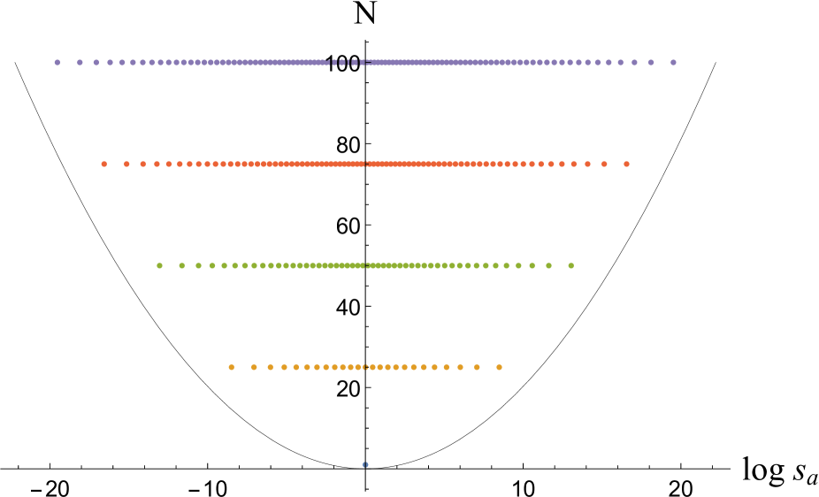
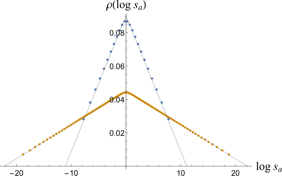
Now we show the numerical results. We used Newton’s method to find the roots of (4.52). For $N\leq 100$, we found that all eigenvalues $s_{a}$ are positive real in our solutions. These eigenvalues can be sorted in ascending order: $y_{a}=0,\quad 0<s_{1}<s_{2}<\ldots<s_{N}$. We also mention that our finite $N$ numerical solutions also satisfy all the assumptions (4.21), (4.24) made in section 4.1 for large $N$ analysis, coming from the eigenvalue distributions not crossing branch cuts. The $N$ eigenvalues spread out from $s_{0}$ ($\rightarrow 1$ in the Cardy limit) with the width roughly proportional to $N^{1/2}$. The detailed eigenvalue distributions at various $N$ are given by Fig. 3. The density of the eigenvalues is defined as $\rho(x)=\frac{1}{N}\frac{da}{dx}$.

(a)

(b)

Figure 4: (a) Imaginary parts of $2\beta\log Z$ (dots) and $2\beta\log Z_{(0)}$ (solid line). (b) Ratio of the finite $N$ free energy $\log Z$ and the fiducial free energy $\log Z_{(0)}$ (dots). Solid line is drawn just as a reference line.

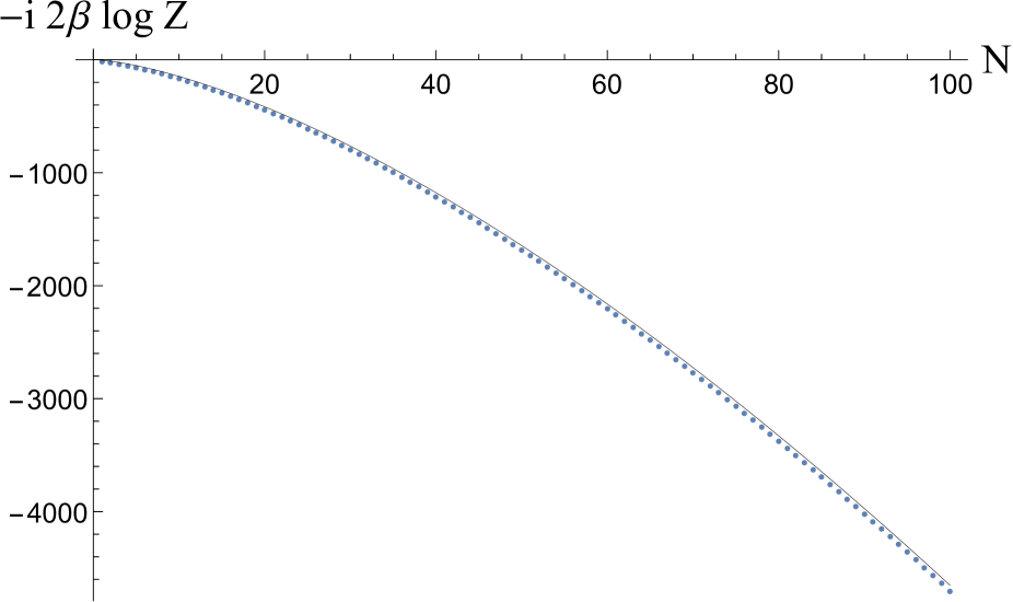
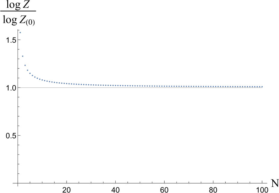
$\log Z_{S^{2}\times S^{1}}$ at various $N$ are given by Fig. 4. One finds that the large $N$ analytic approximation of section 4.1 is well-fitted with the numerical result at large enough $N$. The difference between the numerical result and the fiducial one in Fig. 4(a) increases as $N$ grows, which seems to scale like $O(N^{\frac{1}{2}})$. In addition, we find that the finite $N$ Cardy free energy ($F=-\textrm{Re}\,(\log Z)$) is always smaller than the fiducial one. Although we do not display the relevant plot here, we found that the numerical result for $\textrm{Re}(\mathcal{W}^{*})$ is also well-fitted to the analytically computed $\mathcal{W}_{0}$ at large enough $N$.

Our numerical solutions for $s_{a}$ are very simple, staying at the positive real axis. One may wonder that such simple distributions are due to the simplified setting $\Delta_{1}=\Delta_{2}=\Delta_{3}=\Delta_{4}$. However, we found that the eigenvalues are positive real even at unequal $\Delta_{I}$’s. As the qualitative behaviors are very similar, we shall not plot the results for unequal $\Delta_{I}$’s here.

As long as we are aware of, our results are first quantitatively explored finite $N$ versions of $N^{\frac{3}{2}}$ on M2-branes. Especially, it will be interesting to see if there are any further implications of the analytic coefficient of (4.60), which should be replacing $N^{\frac{3}{2}}$ at $N=2$.

4.3 ABJM theory at large $N$

In this subsection, we make a similar Cardy approximation with the ABJM model for $N$ M2-branes. We reported some difficulties in section 2 to study the vortex partition function for the ABJM theory on $D_{2}\times S^{1}$, due to the diverse possibilities of anomaly-free boundary conditions. This will be closely related the asymptotic factorization in the Cardy limit which we study here, in the set-up of section 3. Namely, we will have to factorize the integrand in a way that the ‘holomorphic’ and ‘anti-holomorphic’ factors separately do not respect the $U(N)\times U(N)$ Weyl symmetry.

The ABJM index on $S^{2}\times S^{1}$ is given by [18]

$$Z_{S^{2}\times S^{1}} =\frac{1}{(N!)^{2}}\!\!\sum_{m_{a},\tilde{m}_{a}\in\mathbb{Z}^{N}}\oint\prod_{a=1}^{N}\left[\frac{ds_{a}}{2\pi is_{a}}\frac{d\tilde{s}_{a}}{2\pi i\tilde{s}_{a}}s_{a}^{km_{a}}\tilde{s}_{a}^{-k\tilde{m}_{a}}\right]q^{\sum_{a,b}|m_{a}-\tilde{m}_{b}|-\frac{1}{2}\sum_{a,b}|m_{a}-m_{b}|-\frac{1}{2}\sum_{a,b}|\tilde{m}_{a}-\tilde{m}_{b}|}$$

$$\times\left[\prod_{a\neq b}^{N}\left(1-s_{a}s_{b}^{-1}q^{|m_{a}-m_{b}|}\right)\right]\left[\prod_{a\neq b}^{N}\left(1-\tilde{s}_{a}\tilde{s}_{b}^{-1}q^{|\tilde{m}_{a}-\tilde{m}_{b}|}\right)\right]$$

$$\times\left[\prod_{A=1}^{2}\prod_{a=1}^{N}\prod_{b=1}^{N}\frac{(s_{a}^{-1}\tilde{s}_{b}t_{A}^{-1}q^{\frac{3}{2}+|m_{a}-\tilde{m}_{b}|};q^{2})}{(s_{a}\tilde{s}_{b}^{-1}t_{A}q^{\frac{1}{2}+|m_{a}-\tilde{m}_{b}|};q^{2})}\right]\left[\prod_{B=3}^{4}\prod_{a=1}^{N}\prod_{b=1}^{N}\frac{(s_{a}\tilde{s}_{b}^{-1}t_{B}^{-1}q^{\frac{3}{2}+|-m_{a}+\tilde{m}_{b}|};q^{2})}{(s_{a}^{-1}\tilde{s}_{b}t_{B}q^{\frac{1}{2}+|-m_{a}+\tilde{m}_{b}|};q^{2})}\right]$$ (4.65)

where $\prod_{I=1}^{4}t_{I}=1$, and again $q=e^{-\beta}$. Note that one of the charges conjugate to $t_{I}$’s is the topological $U(1)$ charge $\sum_{a=1}^{N}(m_{a}+\tilde{m}_{a})$, so a priori it cannot by introduced as rotating elementary fields as shown in this formula. However, by suitably rotating $s_{a}$ and $\tilde{s}_{a}$ by $U(1)^{2}\subset U(N)^{2}$, one can absorb it in into a component of $t_{A}$’s, as shown above.

Before proceeding, we need to comment on the periodicities of chemical potentials. $t_{I}$ and $q=e^{-\beta}$ are related to our previous chemical potentials $\Delta_{I}$ by

$$t_{I}=e^{-\Delta_{I}+\frac{\beta}{2}}\ \ ,\ \ 2\beta=\sum_{I=1}^{4}\Delta_{I}\ (\textrm{mod }4\pi i)\ .$$ (4.66)

One may first insert this expression to (4.3) to eliminate $t_{I}$’s. Then, inserting $\beta=\frac{1}{2}\sum_{I=1}^{4}\Delta_{I}$, one can eliminate $\beta$ to express $Z_{S^{2}\times S^{1}}$ as a function of four independent $\Delta_{I}$’s. After this insertion, one can again identify the expected periodicities (3.16), i.e. shifting any chosen pair of $\Delta_{I}$’s by $(\Delta_{I},\Delta_{J})\rightarrow(\Delta_{I}+2\pi i,\Delta_{J}\pm 2\pi i)$. These are the naturally expected periodicities from the kinematic considerations of the M2-brane QFT. Namely, note from (3.17) that $\Delta_{I}$ is conjugate to the $SO(8)\times SO(3)$ angular momenta $Q_{I}+J$, and also that observables in the spinor representation of $SO(8)$ are also spinor in the spacetime $SO(3)$ in this QFT. These naturally demand the periodicity (3.17) for any thermal partition functions of this QFT, since they are the intrinsic symmetries of the QFT. However, the index (4.3) also has emergent periodicities. Namely, let us define constrained variables $\lambda_{I}$’s by $t_{I}\equiv e^{i\lambda_{I}}$. $\lambda_{I}$ satisfy $\sum_{I=1}^{4}\lambda_{I}=0$ (mod $2\pi$). The emergent symmetry of (4.3) is given by the four independent shifts of $\lambda_{I}$ by $2\pi$, holding $\beta$ fixed. Since (4.3) contains no fractional powers of $t_{I}$, these shifts are obviously symmetries. The symmetries and constraints are summarized as

$$\lambda_{I}\sim\lambda_{I}+2\pi\ \ ,\ \ \ \sum_{I=1}^{4}\lambda_{I}=0\ (\textrm{mod }2\pi)\ .$$ (4.67)

The ‘mod $2\pi$’ in the constraint is also an emergent one, related to the emergent symmetries of $\lambda_{I}$. The symmetry has been used in [10] in the context of the topological index of the ABJM theory, to make a large $N$ analysis. It will turn out below that similar procedures will be applicable to our large $N$ Cardy free energy.

In the Cardy limit, $\Delta_{I}$’s are imaginary and $\lambda_{I}$’s are real. Following [10], we first use the period shifts of $\lambda_{I}$’s to set

$$0<\lambda_{I}<2\pi$$ (4.68)

for all $I=1,\cdots,4$. Then from (4.67), these variables should satisfy one of the following constraints:

$$\sum_{I}\lambda_{I}=2\pi\ ,\ \ 4\pi\ ,\ \ 6\pi\ .$$ (4.69)

If the right hand side is either $0$ or $8\pi$, the resulting free energy is trivial. This is because all $\lambda_{I}$’s are then $0$ up to $2\pi$ shifts, in which case the Cardy behavior $\log Z_{S^{2}\times S^{1}}\propto\beta^{-1}$ is never visible due to boson/fermion cancelations. It will turn out that, following the studies of [10], only the two cases with the right hand side being $2\pi$ and $6\pi$ have nontrivial large $N$ Cardy saddle points. The case with $\sum_{I}\lambda_{I}=2\pi$ will turn out to be the case II of (4.2) in the section 4.1. The case with $\sum_{I}\lambda_{I}=6\pi$ is equivalent to the case I in section 4.1, after shifting all $\lambda_{I}$’s by $-2\pi$. The two cases yield mutually complex conjugate saddle points, as in section 4.1. Below, we shall only consider the case II with $\sum_{I}\lambda_{I}=2\pi$.

Assuming $0<\lambda_{I}<2\pi$, $\sum_{I}\lambda_{I}=2\pi$, we again apply the identity (3.4) to various factors in (4.3), to remove the absolute values of $|\rho(m,\hat{m})|$. As explained below (3.4), there are two ways of removing $|\rho(m)|$, either as $-\rho(m)$ or $+\rho(m)$. For our purpose, the following choices turn out to be useful:

$$|m_{a}-\tilde{m}_{b}| \rightarrow\left\{\begin{array}[]{ll}-(m_{a}-\tilde{m}_{b}),&a\geq b,\\ +(m_{a}-\tilde{m}_{b}),&a<b,\end{array}\right.$$ (4.72)

$$|-m_{a}+\tilde{m}_{b}| \rightarrow\left\{\begin{array}[]{ll}+(-m_{a}+\tilde{m}_{b}),&a\geq b,\\ -(-m_{a}+\tilde{m}_{b}),&a<b.\end{array}\right.$$ (4.75)

We take the Cardy limit of this index assuming the above manipulations, again making the continuum approximation of the monopole sums. This leads to the following factorization into holomorphic and anti-holomorphic parts,

$$Z_{S^{2}\times S^{1}}\sim Z_{\text{hol}}\,Z_{\text{anti-hol}}\ \ ,\ \ \ Z_{\text{hol}}=\int ds_{a}e^{-\frac{\mathcal{W}}{2\beta}},\qquad Z_{\text{anti-hol}}=\int d\bar{s}_{a}e^{\frac{\overline{\mathcal{W}}}{2\beta}}$$ (4.76)

where

$$\mathcal{W} = \frac{k}{2}\left(\sum_{a=1}^{N}u_{a}^{2}-\sum_{b=1}^{N}\tilde{u}_{b}^{2}\right)+\sum_{a<b}\left[\mathrm{Li}_{2}(\tilde{s}_{a}s_{b}^{-1}t_{1,2}^{-1})-\mathrm{Li}_{2}(s_{a}\tilde{s}_{b}^{-1}t_{1,2})+\mathrm{Li}_{2}(s_{a}\tilde{s}_{b}^{-1}t_{3,4}^{-1})-\mathrm{Li}_{2}(\tilde{s}_{a}s_{b}^{-1}t_{3,4})\right]$$ (4.77)

$$+\sum_{a=1}^{N}\left[\mathrm{Li}_{2}(\tilde{s}_{a}s_{a}^{-1}t_{1,2}^{-1})-\mathrm{Li}_{2}(\tilde{s}_{a}s_{a}^{-1}t_{3,4})\right]$$

with the redefinition of the holonomy variable

$$s_{a}q^{m_{a}}\rightarrow s_{a}.$$ (4.78)

Note that the real part of $u_{a}=\log s_{a}$ is identified with $-\beta m_{a}$. We have made a Cardy factorization so that each $\mathcal{W}$, $\overline{\mathcal{W}}$ does not respect $U(N)\times U(N)$ gauge symmetry. This is because we made inequivalent manipulations for the upper-triangular and lower-triangular elements of the matrix-valued fields in (4.72). The reason for this ugly factorization will be clear shortly.

Taking large $N$ limit together with our Cardy limit, we introduce an ansatz

$$u(x)=N^{\alpha}x+iy(x),\qquad\tilde{u}_{a}=N^{\alpha}x+i\tilde{y}(x)$$ (4.79)

with the density function $\rho(x)\geq 0$. Then the large $N$ approximation of (4.77) is given by

$$\mathcal{W} =-ikN^{1+\alpha}\int dx\rho(x)x(\tilde{y}-y)+N^{2-\alpha}\int dx\rho(x)^{2}\left[f(i(\tilde{y}-y+\lambda_{3,4}))-f(i(\tilde{y}-y-\lambda_{1,2}))\right]$$

$$-N\int dx\rho(x)\left[\mathrm{Li}_{2}(e^{i(\tilde{y}-y+\lambda_{3,4})})-\mathrm{Li}_{2}(e^{i(\tilde{y}-y-\lambda_{1,2})})\right]$$ (4.80)

where

$$f(x)=\frac{\{x\}^{3}}{6}-\frac{i\pi}{2}\{x\}^{2}-\frac{\pi^{2}}{3}\{x\},$$ (4.81)

$$\{x\}=\left\{\begin{array}[]{ll}x-2\pi i\left\lfloor\frac{\mathrm{Im}(x)}{2\pi}\right\rfloor,&\mathrm{Re}(x)\leq 0,\\ x-2\pi i\left\lceil\frac{\mathrm{Im}(x)}{2\pi}-1\right\rceil,&\mathrm{Re}(x)>0.\end{array}\right.$$ (4.84)

The last line of (4.3) is subleading in $N$ but plays a role when we consider the equations of motion for the holonomy eigenvalues, i.e., the derivatives of $\mathcal{W}$ [10]. Indeed, it gives rise to a repulsive force such that $\delta y(x)\equiv\tilde{y}(x)-y(x)$ cannot cross $\lambda_{1,2},\,-\lambda_{3,4}$ and their periodic images. Nevertheless, it is not important for the final result once we obtain the extremization solution.

To obtain (4.3), it was important to make a gauge-non-invariant factorization starting from (4.72). Otherwise, there will be a term in $\mathcal{W}$ proportional to $N^{2}$ which furthermore depends on $\rho(x)$. Then it will be very difficult to set up the extremization problem of $\rho(x)$ within the holomorphic part. This is because the leading holomorphic part proportional to $N^{2}$ will cancel with the anti-holomorphic part, so one should keep track of the subleading $N^{\frac{3}{2}}$ term which does not cancel and becomes the leading term of $\log Z_{S^{2}\times S^{1}}$. To summarize, the reason for our ugly factorization is to avoid unwanted terms proportional to $N^{2}$ in our variational problem.

The saddle point is obtained by extremizing $\mathcal{W}$ with respect to $\rho(x)$ and $\delta y(x)$ under the constraint $\int dx\rho(x)=1$. Our prime interest is the case with $k=1$, which we consider first. Remarkably, at $k=1$, this extremization problem is exactly that addressed in [10] for the topologically twisted index. We choose

$$\begin{gathered}0<\delta y(x)+\lambda_{3,4}<2\pi,\quad-2\pi<\delta y(x)-\lambda_{1,2}<0,\\ \lambda_{1}\leq\lambda_{2},\qquad\lambda_{3}\leq\lambda_{4}.\end{gathered}$$ (4.87)

In this range, the second term of (4.3) proportional to $N^{2-\alpha}$ becomes

$$-iN^{2-\alpha}\int dx\rho(x)^{2}\left[g_{+}\left(\delta y(x)+\lambda_{3,4}\right)-g_{-}\left(\delta y(x)-\lambda_{1,2}\right)\right]$$ (4.88)

where

$$g_{\pm}(x)=\frac{x^{3}}{6}\mp\frac{\pi}{2}x^{2}+\frac{\pi^{2}}{3}x.$$ (4.89)

The nontrivial solution is obtained when the first line and the second lines are balanced. Thus, we take $\alpha=\frac{1}{2}$. Then we recognize that

$$\mathcal{W}+i\mu N^{\frac{3}{2}}\left(\int dx\rho(x)-1\right)$$ (4.90)

is exactly $-\mathcal{V}$ in [10] up to the definition of the parameters. (See (2.60) in [10].) By extremizing this functional with $\rho(x)$ and $\delta y(x)$, the solution is given by

$$\begin{array}[]{ll}\begin{array}[]{l}\rho(x)=\frac{\mu+x\lambda_{3}}{(\lambda_{1}+\lambda_{3})(\lambda_{2}+\lambda_{3})(\lambda_{4}-\lambda_{3})},\\ \delta y(x)=-\lambda_{3},\end{array}&x_{\ll}<x<x_{<},\\ \\ \begin{array}[]{l}\rho(x)=\frac{2\pi\mu+x(\lambda_{3}\lambda_{4}-\lambda_{1}\lambda_{2})}{(\lambda_{1}+\lambda_{3})(\lambda_{2}+\lambda_{3})(\lambda_{1}+\lambda_{4})(\lambda_{2}+\lambda_{4})},\\ \delta y(x)=\frac{\mu(\lambda_{1}\lambda_{2}-\lambda_{3}\lambda_{4})+x\sum_{A<B<C}\lambda_{A}\lambda_{B}\lambda_{C}}{2\pi\mu+x(\lambda_{3}\lambda_{4}-\lambda_{1}\lambda_{2})},\end{array}&x_{<}<x<x_{>},\\ \\ \begin{array}[]{l}\rho(x)=\frac{\mu-x\lambda_{1}}{(\lambda_{1}+\lambda_{3})(\lambda_{1}+\lambda_{4})(\lambda_{2}-\lambda_{1})},\\ \delta y(x)=\lambda_{1},\end{array}&x_{>}<x<x_{\gg},\end{array}$$ (4.102)

where

$$x_{\ll}=-\frac{\mu}{\lambda_{3}},\qquad x_{<}=-\frac{\mu}{\lambda_{4}},\qquad x_{>}=\frac{\mu}{\lambda_{2}},\qquad x_{\gg}=\frac{\mu}{\lambda_{1}},\qquad\mu=\sqrt{2\lambda_{1}\lambda_{2}\lambda_{3}\lambda_{4}},$$ (4.103)

Substituting the solution back to $\mathcal{W}$, one obtains

$$\mathcal{W}^{\ast}=-\frac{iN^{\frac{3}{2}}\mu^{3}}{3\lambda_{1}\lambda_{2}\lambda_{3}\lambda_{4}}=-\frac{2\sqrt{2}N^{\frac{3}{2}}}{3}i\sqrt{\lambda_{1}\lambda_{2}\lambda_{3}\lambda_{4}}$$ (4.104)

and moreover

$$\log Z_{\text{hol}}=-\frac{\mathcal{W}^{\ast}}{2\beta}=\frac{\sqrt{2}N^{\frac{3}{2}}}{3\beta}i\sqrt{\lambda_{1}\lambda_{2}\lambda_{3}\lambda_{4}}\ ,\ \ \log Z_{\text{anti-hol}}=\frac{\overline{\mathcal{W}}^{\ast}}{2\beta}=\frac{\sqrt{2}N^{\frac{3}{2}}}{3\beta}i\sqrt{\lambda_{1}\lambda_{2}\lambda_{3}\lambda_{4}}\ .$$ (4.105)

Combining these two, one obtains the large $N$ Cardy free energy given by

$$\log Z_{S^{2}\times S^{1}}\sim\log Z_{\text{hol}}+\log Z_{\text{anti-hol}}\sim\frac{2\sqrt{2}N^{\frac{3}{2}}}{3\beta}i\sqrt{\Delta_{1}\Delta_{2}\Delta_{3}\Delta_{4}}$$ (4.106)

with $\sum_{I=1}^{4}\Delta_{I}-2\beta=-2\pi i$. This indeed agrees with the results in section 4.1 in the region II. Similar studies can be made in the region I, providing the complex conjugate results.

For generic $k$, one can easily obtain the result by replacing $\rho(x)$ by $k\hat{\rho}(x)$ in the previous computation. Then one finds

$$\mathcal{W}(x,y,\rho)=k^{2}\mathcal{W}_{k=1}(x,y,\hat{\rho})\ .$$ (4.107)

So most of the previous calculations at $k=1$ can be used here, except that $\mu$ has to be tuned differently to match the constraint $\int dx\hat{\rho}(x)=\frac{1}{k}$. The modified value for $\mu$ turns out to be $\mu=\sqrt{\frac{2\lambda_{1}\lambda_{2}\lambda_{3}\lambda_{4}}{k}}$. Plugging all these into $\mathcal{W}$, one obtains $\mathcal{W}^{\ast}=-\frac{ik^{2}N^{\frac{3}{2}}\mu^{3}}{3\lambda_{1}\lambda_{2}\lambda_{3}\lambda_{4}}=-\frac{2\sqrt{2}k^{\frac{1}{2}}N^{\frac{3}{2}}}{3}i\sqrt{\lambda_{1}\lambda_{2}\lambda_{3}\lambda_{4}}$ and accordingly

$$\log Z_{S^{2}\times S^{1}}\sim\frac{2\sqrt{2}k^{\frac{1}{2}}N^{\frac{3}{2}}}{3\beta}i\sqrt{\lambda_{1}\lambda_{2}\lambda_{3}\lambda_{4}}=\frac{2\sqrt{2}k^{\frac{1}{2}}N^{\frac{3}{2}}}{3\beta}i\sqrt{\Delta_{1}\Delta_{2}\Delta_{3}\Delta_{4}}\ .$$ (4.108)

5 Conclusion and remarks

In this paper, we explored the Cardy limit of the index for the M2-brane SCFTs on $S^{2}\times\mathbb{R}$. Our studies are made by analyzing the vortex partition functions, and also suitably approximating the GNO charge sum for the magnetic monopole operators. At large $N$, we have quantitatively shown that the deconfined free energy scales like $N^{\frac{3}{2}}$. This free energy statistically accounts for the Bekenstein-Hawking entropies of large BPS black holes in $AdS_{4}\times S^{7}$. We discovered the important roles played by the condensation of magnetic monopole operators, which provides a mechanism for partial confinement of $N^{2}$ degrees of freedom. We have also found finite $N$ versions of $N^{\frac{3}{2}}$ degrees of freedom by studying the Cardy limit of the index.

We believe that these discoveries will shed very concrete lights on the strongly interacting dynamics of 3d (S)CFTs, including the M2-brane CFTs.

One important issue that has been treated rather briefly in this paper is the exclusion behavior of eigenvalues in our index. This phenomenon has been first explored in the 3d vector-Chern-Simons theories, either using semi-classical arguments [29] or based on path integral approach [30]. We employed the strategy of [30] and studied the index of our M2-brane QFT. The key result is that the GNO charge sum forbids eigenvalues to assume same values, not even asymptotically in the high temperature limit. In the vector-Chern-Simons model, this phenomenon played important roles to make certain dualities to hold. In our M2-brane QFT, similar exclusion principle forbids the naive saddle point whose free energy is proportional to $N^{2}$. Both in the study of [30] and this paper, there are further issues to clarify concerning the small spreading of the delta functions of $\alpha_{a}$’s, as explained in the conclusion of [30].

As a technical remark, we mainly used the $\mathcal{N}=4$ Yang-Mills-matter theory engineered on the D2-D6-brane system, rather than the ABJM theory. When we first started our project, this was because we were aiming to use the vortex partition function in the Higgs branch and the factorization of $Z_{S^{2}\times S^{1}}$. In Chern-Simons-matter theories, studies of vortex partition functions are more difficult. Apparently, this seems to be due to the difficulty in finding natural anomaly-free boundary condition on $D_{2}\times S^{1}$. More physically, with Chern-Simons terms, there may be so-called non-topological vortices in the symmetric phase, apart from the topological vortices in the Higgs phase. This is because once we have electrically charged configurations in the symmetric phase, magnetic flux is induced due to the Gauss’ law of Chern-Simons-matter theory. It is natural that these non-topological vortices may play roles in the factorization formulae of the ABJM theory, if there is one at all. However, our alternative asymptotic factorization of section 3 (in the Cardy limit) can be applied to the ABJM theory, as we explained in section 4.3.

Acknowledgements

We thank Hee-Cheol Kim, Joonho Kim, Kimyeong Lee, Sungjay Lee, Shiraz Minwalla, June Nahmgoong, Jaemo Park, Shuichi Yokoyama and especially Dongmin Gang for helpful discussions. This work is supported in part by the National Research Foundation of Korea Grant 2018R1A2B6004914 (SC, SK), NRF-2017-Global Ph.D. Fellowship Program (SC), the ERC-STG grant 637844-HBQFTNCER (CH) and the INFN (CH).

Appendix A Asymptotic behavior of $q$-Pochhammer symbols

From [44], we get the following asymptotic formulae of $q$-Pochhammer symbols for $|a|\leq 1$;

$$(aq^{m};q^{2})_{\infty}=\prod_{n=0}^{\infty}(1-aq^{m+2n}),\quad q=e^{-\beta}\;(|q|<1)\ ,$$ (A.1)

$$\lim_{\beta\to 0^{+}}(aq^{m};q^{2})_{\infty}=\,(1-aq^{m})^{1/2}\,\exp\Big{[}-\frac{1}{2\beta}\textrm{Li}_{2}(aq^{m})\Big{]}\big{(}1+o({\beta}^{0})\big{)},\quad|a|\leq 1\;\&\;a\neq 1\;(a\in\mathbb{C}),$$

$$\lim_{\beta\to 0^{+}}(q^{m};q^{2})_{\infty}=\frac{\sqrt{2\pi}}{\Gamma(m/2)}(2\beta)^{-(m-1)/2}\exp\Big{[}-\frac{1}{2\beta}\textrm{Li}_{2}(1)\Big{]}\big{(}1+o({\beta}^{0})\big{)}.$$

We will extend the above asymptotic formulae to the whole complex plane $\mathbb{C}$ with the help of the Jacobi theta function and the Dedekind eta function:

$$\theta_{1}(\tau,z)=-e^{\frac{i\pi}{2}}y^{\frac{1}{2}}\tilde{q}^{\frac{1}{8}}\prod_{n=1}^{\infty}(1-\tilde{q}^{n})(1-y\tilde{q}^{n})(1-y^{-1}\tilde{q}^{n-1})=-e^{\frac{i\pi}{2}}y^{\frac{1}{2}}\tilde{q}^{\frac{1}{8}}(\tilde{q};\tilde{q})_{\infty}(y\tilde{q};\tilde{q})_{\infty}(y^{-1};\tilde{q})_{\infty},$$ (A.2)

$$\eta(\tau)=\tilde{q}^{\frac{1}{24}}\prod_{n=1}^{\infty}(1-\tilde{q}^{n})=\tilde{q}^{\frac{1}{24}}(\tilde{q};\tilde{q})_{\infty},\quad\tilde{q}=e^{2\pi i\tau}\;(\tau\in\mathbb{C}\;\&\;\textrm{Im}(\tau)>0),\;y=e^{2\pi iz}\;(z\in\mathbb{C}).$$

These functions have the following modular properties:

$$\theta_{1}(-\frac{1}{\tau},\frac{z}{\tau})=-i(-i\tau)^{1/2}\exp\Big{(}i\frac{\pi}{\tau}z^{2}\Big{)}\theta_{1}(\tau,z),$$ (A.3)

$$\eta(-\frac{1}{\tau})=(-i\tau)^{1/2}\eta(\tau).$$

Now we relate the parameters appearing in (A.1) and (A.2) as

$$\tilde{q}=q^{2}=e^{-2\beta},\;\beta>0\;\Rightarrow\;\tau=\frac{i\beta}{\pi},\;\textrm{Re}(\tau)=0,\;\textrm{Im}(\tau)>0,$$ (A.4)

$$y=a\in\mathbb{C},\;|a|\leq 1\;\&\;a\neq 0,\,1\;\Rightarrow\;z=\frac{\log a}{2\pi i},\;-\pi\leq\textrm{Arg}(a)\leq\pi.$$

Then, one finds that

$$(a^{-1};q^{2})_{\infty} =-e^{-\frac{i\pi}{2}}a^{-\frac{1}{2}}q^{-\frac{1}{6}}\frac{\theta_{1}(\tau,z)}{\eta(\tau)(aq^{2};q^{2})_{\infty}}$$ (A.5)

$$=-\frac{1-a}{a^{1/2}}q^{-\frac{1}{6}}\exp\Big{(}\frac{(\log a)^{2}}{4\beta}\Big{)}\frac{\theta_{1}(-\frac{1}{\tau},\frac{z}{\tau})}{\eta(-\frac{1}{\tau})(a;q^{2})_{\infty}}.$$

Taking $\beta\to 0^{+}$ limit, one obtains

$$(a^{-1};q^{2})_{\infty}= -(a^{-1}-1)^{1/2}\frac{\theta_{1}(-\frac{1}{\tau},\frac{z}{\tau})}{\eta(-\frac{1}{\tau})}\,\exp\bigg{[}\frac{1}{2\beta}\Big{(}\textrm{Li}_{2}(a)+\frac{1}{2}(\log a)^{2}\Big{)}+\frac{\beta}{6}\bigg{]}\big{(}1+o({\beta}^{0})\big{)}$$ (A.6)

$$= (a^{-1}-1)^{1/2}\exp\bigg{[}\frac{1}{2\beta}\Big{(}\textrm{Li}_{2}(a)+\frac{1}{2}(\log a)^{2}-\frac{\pi^{2}}{3}\Big{)}\bigg{]}$$

$$2\frac{(e^{i\pi\frac{\log a}{2\beta}}-e^{-i\pi\frac{\log a}{2\beta}})}{2i}\prod_{n=1}^{\infty}(1-e^{-i\pi\frac{\log a}{\beta}-\frac{2n\pi^{2}}{\beta}})(1-e^{i\pi\frac{\log a}{\beta}-\frac{2n\pi^{2}}{\beta}})\big{(}1+o({\beta}^{0})\big{)}$$

$$= (a^{-1}-1)^{1/2}\exp\bigg{[}\frac{1}{2\beta}\Big{(}\textrm{Li}_{2}(a)+\frac{1}{2}(\log a)^{2}-\frac{\pi^{2}}{3}\Big{)}\bigg{]}\bigg{(}2\frac{(e^{i\pi\frac{\log a}{2\beta}}-e^{-i\pi\frac{\log a}{2\beta}})}{2i}\bigg{)}\big{(}1+o({\beta}^{0})\big{)}.$$

For $|a|\leq 1\;\&\;a\notin[0,1]\;(a\in\mathbb{C})$, this is simplified as

$$(a^{-1};q^{2})_{\infty}= (1-a^{-1})^{1/2}\exp\bigg{[}\frac{1}{2\beta}\Big{(}\textrm{Li}_{2}(a)+\frac{1}{2}(\log(-a))^{2}+\frac{\pi^{2}}{6}\Big{)}\bigg{]}\big{(}1+o({\beta}^{0})\big{)}$$ (A.7)

$$= (1-a^{-1})^{1/2}\exp\bigg{[}-\frac{1}{2\beta}\textrm{Li}_{2}(a^{-1})\bigg{]}\big{(}1+o({\beta}^{0})\big{)},\quad|a|\leq 1\;\&\;a\notin[0,1]\;(a\in\mathbb{C}).$$

So we find the following asymptotic formulae of $q$-Pochhammer symbols:

$$\lim_{\beta\to 0^{+}}(aq^{m};q^{2})_{\infty} =\,(1-aq^{m})^{1/2}\,\exp\Big{[}-\frac{1}{2\beta}\textrm{Li}_{2}(aq^{m})\Big{]}\big{(}1+o({\beta}^{0})\big{)}$$ (A.8)

$$=\exp\left[-\frac{1}{2\beta}{\rm Li}_{2}(aq^{m-1})\right]\left(1+o(\beta^{0})\right),\quad a\in\mathbb{C}\;\&\;a\notin[1,\infty),$$

$$\lim_{\beta\to 0^{+}}(q^{m};q^{2})_{\infty} =\,\frac{\sqrt{2\pi}}{\Gamma(m/2)}(2\beta)^{-(m-1)/2}\,\exp\Big{[}-\frac{1}{2\beta}\textrm{Li}_{2}(1)\Big{]}\big{(}1+o({\beta}^{0})\big{)}\quad(a=1).$$

Appendix B Young diagram formula for $Z_{\rm vortex}$

In section 2.1, we encountered the following formula

$$Z_{\rm vortex}=\!\!\!\!\sum_{0\leq k_{1}\leq\cdots\leq k_{N}}\!\!\!Q^{k_{1}+\cdots+k_{N}}\prod_{a=1}^{N}\frac{(v^{-a+1};q^{2})_{-k_{a}}}{(u^{-2}v^{-a+1};q^{2})_{-k_{a}}}\cdot\prod_{a,b=1\ (a\neq b)}^{N}\frac{(v^{-a+b+1};q^{2})_{-k_{a}+k_{b}}(u^{-2}v^{-a+b}q^{2};q^{2})_{-k_{a}+k_{b}}}{(v^{-a+b};q^{2})_{-k_{a}+k_{b}}(u^{-2}v^{-a+b+1}q^{2};q^{2})_{-k_{a}+k_{b}}}$$ (B.1)

for the vortex partition function. In this appendix, we prove the Young diagram formula (2.25) for $Z_{\rm vortex}$.

Note that $(k_{N},\ldots,k_{1})$ is a set of non-increasing non-negative integers. Thus, it can be represented by a Young diagram, $\lambda=(\lambda_{1},\ldots,\lambda_{N})$, where each $\lambda_{i}$ is defined by $\lambda_{i}=k_{N-i+1}$. In terms of $\lambda_{i}$, (B.1) is written as

$$\sum_{\lambda_{1}\geq\lambda_{2}\geq\ldots\geq\lambda_{N}\geq 0}Q^{|\lambda|}\left(\prod_{i=1}^{N}\frac{(u^{-2}v^{-N+i};q^{-2})_{\lambda_{i}}}{(v^{-N+i}q^{-2};q^{-2})_{\lambda_{i}}}\right)\left(\prod_{i<j}^{N}\frac{(v^{-(j-i)}q^{-2};q^{-2})_{\lambda_{i}-\lambda_{j}}(u^{-2}v^{-(j-i-1)};q^{-2})_{\lambda_{i}-\lambda_{j}}}{(u^{-2}v^{-(j-i)};q^{-2})_{\lambda_{i}-\lambda_{j}}(v^{-(j-i-1)}q^{-2};q^{-2})_{\lambda_{i}-\lambda_{j}}}\right)$$

$$\ \ \ \quad\quad\quad\times\left(\prod_{i<j}^{N}\frac{(u^{-2}v^{j-i}q^{2};q^{2})_{\lambda_{i}-\lambda_{j}}(v^{j-i+1};q^{2})_{\lambda_{i}-\lambda_{j}}}{(v^{j-i};q^{2})_{\lambda_{i}-\lambda_{j}}(u^{-2}v^{j-i+1}q^{2};q^{2})_{\lambda_{i}-\lambda_{j}}}\right)$$

$$=\sum_{\lambda_{1}\geq\lambda_{2}\geq\ldots\geq\lambda_{N}\geq 0}Q^{|\lambda|}\left(\prod_{i=1}^{N}\frac{(u^{-2};q^{-2})}{(q^{-2};q^{-2})}\frac{(u^{-2}vq^{2};q^{2})(v^{N-i+1};q^{2})}{(v;q^{2})(u^{-2}v^{N-i+1}q^{2};q^{2})}\right)\left(\prod_{i=1}^{N}\frac{(v^{-N+i}q^{-2(\lambda_{i}+1)};q^{-2})}{(u^{-2}v^{-N+i}q^{-2\lambda_{i}};q^{-2})}\right)$$

$$\quad\times\left(\prod_{i<j}^{N}\frac{(u^{-2}v^{-(j-i)}q^{-2(\lambda_{i}-\lambda_{j})};q^{-2})(v^{-(j-i-1)}q^{-2(\lambda_{i}-\lambda_{j}+1)};q^{-2})}{(v^{-(j-i)}q^{-2(\lambda_{i}-\lambda_{j}+1)};q^{-2})(u^{-2}v^{-(j-i-1)}q^{-2(\lambda_{i}-\lambda_{j})};q^{-2})}\right)$$

$$\quad\times\left(\prod_{i<j}^{N}\frac{(v^{j-i}q^{2(\lambda_{i}-\lambda_{j})};q^{2})(u^{-2}v^{j-i+1}q^{2(\lambda_{i}-\lambda_{j}+1)};q^{2})}{(u^{-2}v^{j-i}q^{2(\lambda_{i}-\lambda_{j}+1)};q^{2})(v^{j-i+1}q^{2(\lambda_{i}-\lambda_{j})};q^{2})}\right)$$ (B.2)

where we have used

$$(a;q)_{n}=\frac{(a;q)}{(aq^{n};q)}.$$ (B.3)

Note that (B) includes $(a;q^{-2})$, whose analytic continuation should be understood for $|q|<1$ using

$$(a;q^{-2})=\frac{1}{(aq^{2};q^{2})}.$$ (B.4)

Now one can use the following identity [45]

$$\left(\prod_{i=1}^{N}\frac{(x;q)}{(q^{\lambda_{i}}t^{N-i}x;q)}\right)\left(\prod_{i<j}\frac{(q^{\lambda_{i}-\lambda_{j}}t^{j-i}x;q)}{(q^{\lambda_{i}-\lambda_{j}}t^{j-i-1}x;q)}\right)=\prod_{(i,j)\in\lambda}\left(1-q^{\lambda_{i}-j}t^{\lambda^{\prime}_{j}-i}x\right),$$ (B.5)

$$\prod_{i=1}^{N}\frac{(t^{1-i}x;q)}{(q^{\lambda_{i}}t^{1-i}x;q)}=\prod_{(i,j)\in\lambda}\left(1-q^{j-1}t^{1-i}x\right)$$ (B.6)

to obtain

$$Z_{\text{vortex}}=\sum_{\lambda}Q^{|\lambda|}\sum_{(i,j)\in\lambda}\frac{\left(1-u^{-2}v^{-\lambda^{\prime}_{j}+i}q^{-2\lambda_{i}+2j}\right)\left(1-u^{-2}v^{\lambda^{\prime}_{j}-i+1}q^{2\lambda_{i}-2j+2}\right)\left(1-v^{N-i+1}q^{2j-2}\right)}{\left(1-v^{-\lambda^{\prime}_{j}+i}q^{-2\lambda_{i}+2j-2}\right)\left(1-v^{\lambda^{\prime}_{j}-i+1}q^{2\lambda_{i}-2j}\right)\left(1-u^{-2}v^{N-i+1}q^{2j}\right)}$$ (B.7)

where $\lambda^{\prime}$ is the conjugate of $\lambda$. Namely, $\lambda^{\prime}_{j}$ is the vertical length of the $j$th column of $\lambda$ while $\lambda_{i}$ is the horizontal length of the $i$th row of $\lambda$. This proves (2.25).

Recall that the expression (B.7) is obtained under the conditions $|u^{2}|<1,\,|u^{-2}q^{2}|<1,\,|v|<1,\,|Q|<1$ and $|q|<1$; i.e.,

$$\pm T_{*}-\beta<0,\quad f_{*}+\frac{T_{*}}{2}-\frac{\beta}{2}<0,\quad\xi_{*}>0,\quad\beta>0$$ (B.8)

with $\xi=-\log Q$. $x_{*}$ denotes the real part of $x$. In particular, the first condition shows that $|T_{*}|<\beta$. We have numerically checked, by $q$-expansion, that (B.7) is not valid if any of the above inequalities is flipped. (We have checked this at $N=2$.)

As a simple application, let us study study the large $N$ limit of the vortex partition function (2.25). In this case, since $v<1$, we can take $v^{N}$ to zero. Then the large $N$ limit of the vortex partition function is given by

$$Z_{\rm vortex}\stackrel{{\scriptstyle N\rightarrow\infty}}{{\longrightarrow}}\sum_{Y}Q^{|Y|}\prod_{s\in Y}\frac{(1-u^{-2}(q^{2h(s)}v^{v(s)})^{-1})(1-u^{-2}vq^{2}\cdot q^{2h(s)}v^{v(s)})}{(1-q^{-2}(q^{2h(s)}v^{v(s)})^{-1})(1-vq^{2h(s)}v^{v(s)})}$$ (B.9)

where $q=e^{-\beta}$, $u=(qt)^{\frac{1}{2}}=e^{\frac{T-\beta}{2}}$, $v=z(qt)^{\frac{1}{2}}=e^{f+\frac{T-\beta}{2}}$. This series is well known. Upon suitable parameter mappings, this is functionally identical to the instanton partition function of 5d $\mathcal{N}=1^{\ast}$ super-Yang-Mills theory with $U(1)$ gauge group [46]. The $Q$ series of this partition function can be summed to the following expression [47, 48],

$$Z^{N\rightarrow\infty}_{\rm vortex}=PE\left[\frac{(1-u^{-2})(1-u^{-2}vq^{2})}{(1-q^{-2})(1-v)}\frac{Q}{1-q^{2}Qu^{-2}}\right]\ ,$$ (B.10)

where $PE\left[f(Q,q,u,v)\right]\equiv\exp\left[\sum_{n=1}^{\infty}\frac{1}{n}f(Q^{n},q^{n},u^{n},v^{n})\right]$. So $Z_{\rm vortex}$ has smooth large $N$ limit. The perturbative part is given by

$$Z_{\rm pert}=\prod_{a=1}^{N}\frac{(u^{-2}v^{a}q^{2};q^{2})_{\infty}}{(v^{a};q^{2})_{\infty}}=PE\left[\frac{(1-u^{-2}q^{2})(v+v^{2}+\cdots+v^{N})}{1-q^{2}}\right]\ .$$ (B.11)

This also has a smooth large $N$ limit

$$Z_{\rm pert}^{N\rightarrow\infty}=PE\left[-\frac{q^{-2}v(1-u^{-2}q^{2})}{(1-q^{-2})(1-v)}\right]\ .$$ (B.12)

Multiplying $Z_{\rm pert}$ and $Z_{\rm vortex}$, one obtains

$$Z^{N\rightarrow\infty}_{\rm pert}Z^{N\rightarrow\infty}_{\rm vortex}=PE\left[\frac{Q+vu^{-2}+Qvu^{-2}-Qu^{-2}-vq^{-2}-q^{2}Qvu^{-2}}{(1-q^{-2})(1-v)(1-q^{2}Qu^{-2})}\right]\ .$$ (B.13)

As explained in section 2.1, we ignore the $Z_{\rm prefactor}$ factor.

References

- [1] I. R. Klebanov and A. A. Tseytlin, Nucl. Phys. B 475, 164 (1996) doi:10.1016/0550-3213(96)00295-7 [hep-th/9604089].
- [2] N. Drukker, M. Marino and P. Putrov, Commun. Math. Phys. 306, 511 (2011) doi:10.1007/s00220-011-1253-6 [arXiv:1007.3837 [hep-th]].
- [3] C. P. Herzog, I. R. Klebanov, S. S. Pufu and T. Tesileanu, Phys. Rev. D 83, 046001 (2011) doi:10.1103/PhysRevD.83.046001 [arXiv:1011.5487 [hep-th]].
- [4] H. C. Kim and S. Kim, JHEP 1305, 144 (2013) doi:10.1007/JHEP05(2013)144 [arXiv:1206.6339 [hep-th]]; J. Kallen, J. A. Minahan, A. Nedelin and M. Zabzine, JHEP 1210, 184 (2012) doi:10.1007/JHEP10(2012)184 [arXiv:1207.3763 [hep-th]]; G. Lockhart and C. Vafa, arXiv:1210.5909 [hep-th]; H. C. Kim, J. Kim and S. Kim, arXiv:1211.0144 [hep-th]; J. A. Minahan, A. Nedelin and M. Zabzine, J. Phys. A 46, 355401 (2013) doi:10.1088/1751-8113/46/35/355401 [arXiv:1304.1016 [hep-th]]; H. C. Kim, S. Kim, S. S. Kim and K. Lee, arXiv:1307.7660 [hep-th].
- [5] J. A. Harvey, R. Minasian and G. W. Moore, JHEP 9809, 004 (1998) doi:10.1088/1126-6708/1998/09/004 [hep-th/9808060].
- [6] T. Maxfield and S. Sethi, JHEP 1206, 075 (2012) doi:10.1007/JHEP06(2012)075 [arXiv:1204.2002 [hep-th]].
- [7] S. Kim and J. Nahmgoong, JHEP 1712, 120 (2017) doi:10.1007/JHEP12(2017)120 [arXiv:1702.04058 [hep-th]].
- [8] S. Choi, J. Kim, S. Kim and J. Nahmgoong, arXiv:1810.12067 [hep-th].
- [9] J. Nahmgoong, arXiv:1907.12582 [hep-th].
- [10] F. Benini, K. Hristov and A. Zaffaroni, JHEP 1605, 054 (2016) doi:10.1007/JHEP05(2016)054 [arXiv:1511.04085 [hep-th]].
- [11] F. Benini, K. Hristov and A. Zaffaroni, Phys. Lett. B 771, 462 (2017) doi:10.1016/j.physletb.2017.05.076 [arXiv:1608.07294 [hep-th]].
- [12] M. Cvetic, G. W. Gibbons, H. Lu and C. N. Pope, hep-th/0504080.
- [13] K. Hristov, S. Katmadas and C. Toldo, arXiv:1907.05192 [hep-th].
- [14] A. Kapustin, B. Willett and I. Yaakov, JHEP 1010, 013 (2010) doi:10.1007/JHEP10(2010)013 [arXiv:1003.5694 [hep-th]].
- [15] D. Gang, E. Koh, K. Lee and J. Park, arXiv:1108.3647 [hep-th].
- [16] J. Bhattacharya, S. Bhattacharyya, S. Minwalla and S. Raju, JHEP 0802, 064 (2008) doi:10.1088/1126-6708/2008/02/064 [arXiv:0801.1435 [hep-th]].
- [17] J. Bhattacharya and S. Minwalla, JHEP 0901, 014 (2009) doi:10.1088/1126-6708/2009/01/014 [arXiv:0806.3251 [hep-th]].
- [18] S. Kim, Nucl. Phys. B 821, 241 (2009) Erratum: [Nucl. Phys. B 864, 884 (2012)] doi:10.1016/j.nuclphysb.2012.07.015, 10.1016/j.nuclphysb.2009.06.025 [arXiv:0903.4172 [hep-th]].
- [19] S. Choi, C. Hwang, S. Kim and J. Nahmgoong, arXiv:1811.02158 [hep-th].
- [20] A. Cabo-Bizet, D. Cassani, D. Martelli and S. Murthy, arXiv:1810.11442 [hep-th].
- [21] S. Choi, J. Kim, S. Kim and J. Nahmgoong, arXiv:1811.08646 [hep-th].
- [22] F. Benini and P. Milan, arXiv:1812.09613 [hep-th].
- [23] M. Honda, arXiv:1901.08091 [hep-th].
- [24] A. Arabi Ardehali, arXiv:1902.06619 [hep-th].
- [25] J. Kim, S. Kim and J. Song, arXiv:1904.03455 [hep-th].
- [26] A. Cabo-Bizet, D. Cassani, D. Martelli and S. Murthy, arXiv:1904.05865 [hep-th].
- [27] F. Larsen, J. Nian and Y. Zeng, arXiv:1907.02505 [hep-th].
- [28] S. Choi and S. Kim, arXiv:1904.01164 [hep-th].
- [29] O. Aharony, S. Giombi, G. Gur-Ari, J. Maldacena and R. Yacoby, JHEP 1303, 121 (2013) doi:10.1007/JHEP03(2013)121 [arXiv:1211.4843 [hep-th]].
- [30] S. Jain, S. Minwalla, T. Sharma, T. Takimi, S. R. Wadia and S. Yokoyama, JHEP 1309, 009 (2013) doi:10.1007/JHEP09(2013)009 [arXiv:1301.6169 [hep-th]].
- [31] J. Bagger and N. Lambert, Phys. Rev. D 75, 045020 (2007) doi:10.1103/PhysRevD.75.045020 [hep-th/0611108]; J. Bagger and N. Lambert, Phys. Rev. D 77, 065008 (2008) doi:10.1103/PhysRevD.77.065008 [arXiv:0711.0955 [hep-th]].
- [32] A. Gustavsson, Nucl. Phys. B 811, 66 (2009) doi:10.1016/j.nuclphysb.2008.11.014 [arXiv:0709.1260 [hep-th]].
- [33] O. Aharony, O. Bergman, D. L. Jafferis and J. Maldacena, JHEP 0810, 091 (2008) doi:10.1088/1126-6708/2008/10/091 [arXiv:0806.1218 [hep-th]].
- [34] Y. Yoshida and K. Sugiyama, arXiv:1409.6713 [hep-th].
- [35] D. Gaiotto, L. Rastelli and S. S. Razamat, JHEP 1301, 022 (2013) doi:10.1007/JHEP01(2013)022 [arXiv:1207.3577 [hep-th]].
- [36] D. Gaiotto and E. Witten, Adv. Theor. Math. Phys. 13, no. 3, 721 (2009) doi:10.4310/ATMP.2009.v13.n3.a5 [arXiv:0807.3720 [hep-th]].
- [37] H. C. Kim, J. Kim, S. Kim and K. Lee, arXiv:1204.3895 [hep-th].
- [38] S. Pasquetti, JHEP 1204 (2012) 120 [arXiv:1111.6905 [hep-th]]; C. Beem, T. Dimofte and S. Pasquetti, JHEP 1412 (2014) 177 [arXiv:1211.1986 [hep-th]]; C. Hwang, H. C. Kim and J. Park, JHEP 1408 (2014) 018 [arXiv:1211.6023 [hep-th]]; M. Taki, arXiv:1303.5915 [hep-th]; M. Fujitsuka, M. Honda and Y. Yoshida, PTEP 2014 (2014) no.12, 123B02 [arXiv:1312.3627 [hep-th]]; F. Benini and W. Peelaers, JHEP 1405 (2014) 030 [arXiv:1312.6078 [hep-th]]; F. Benini and A. Zaffaroni, JHEP 1507 (2015) 127 [arXiv:1504.03698 [hep-th]]; C. Hwang and J. Park, JHEP 1511 (2015) 028 [arXiv:1506.03951 [hep-th]].
- [39] C. Hwang, H. Kim and J. Park, arXiv:1807.06198 [hep-th].
- [40] Y. Imamura and S. Yokoyama, JHEP 1104 (2011) 007 doi:10.1007/JHEP04(2011)007 [arXiv:1101.0557 [hep-th]].
- [41] T. Dimofte, D. Gaiotto and S. Gukov, Adv. Theor. Math. Phys. 17, no. 5, 975 (2013) doi:10.4310/ATMP.2013.v17.n5.a3 [arXiv:1112.5179 [hep-th]].
- [42] S. Pasquetti and M. Sacchi, arXiv:1903.10817 [hep-th].
- [43] O. Aharony, J. Marsano, S. Minwalla, K. Papadodimas and M. Van Raamsdonk, Adv. Theor. Math. Phys. 8, 603 (2004) doi:10.4310/ATMP.2004.v8.n4.a1 [hep-th/0310285].
- [44] S. Fredenhagen and V. Schomerus, JHEP 0505, 025 (2005) [arXiv:hep-th/0409256].
- [45] Rains, E. M. 2001, arXiv Mathematics e-prints, math/0112035
- [46] N. A. Nekrasov, Adv. Theor. Math. Phys. 7, no. 5, 831 (2003) doi:10.4310/ATMP.2003.v7.n5.a4 [hep-th/0206161].
- [47] A. Iqbal, C. Kozcaz and K. Shabbir, Nucl. Phys. B 838, 422 (2010) doi:10.1016/j.nuclphysb.2010.06.010 [arXiv:0803.2260 [hep-th]].
- [48] H. C. Kim, S. Kim, E. Koh, K. Lee and S. Lee, JHEP 1112, 031 (2011) doi:10.1007/JHEP12(2011)031 [arXiv:1110.2175 [hep-th]].