A Search for Variable Stars in the Globular Cluster M4 with K2

Abstract

We extract light curves for 4554 objects with $9{<}G{<}19$ in the K2 superstamp observations of the globular cluster M4, including 3784 cluster members, and search for variability. Among cluster member objects, we detect 66 variables, of which 52 are new discoveries. Among objects not belonging to the cluster, we detect 24 variables, of which 20 are new discoveries. We additionally discover 57 cluster-member suspected variables, 10 cluster-non-member suspected variables, and four variables with ambiguous cluster membership. Our light curves reach sub-millimagnitude precision for the cluster horizontal branch, permitting us to detect asteroseismic activity in six horizontal branch stars outside the instability strip and one inside the strip but with only ${\sim}$1 mmag amplitude variability. 19 additional stars along the red giant branch also have detected asteroseismic variability. Several eclipsing binaries are found in the cluster, including a 4.6-day detached eclipsing binary and an EW-class eclipsing binary, as well as an EW with uncertain cluster membership and three other candidate EWs. A 22-day detached eclipsing binary is also found outside the cluster. We identify a candidate X-ray binary that is a cluster member with quiescent and periodic ${\sim}$20 mmag optical variability. We also obtain high-precision light curves for ten of the previously known RR Lyrae variables in the cluster and identify one as a candidate Blazhko variable with a Blazhko period in excess of 78 days. We make our light curves publicly available.

1 Introduction

The globular cluster (GC) M4 (NGC 6121), located in the constellation Scorpius, is the closest GC to Earth at a distance of ${\sim}$1.8 kpc (Kaluzny et al. 2013b; Braga et al. 2015; Neeley et al. 2015). M4 is an old GC, with recent age measurements falling between ${\sim}$11–12 Gyr (Bedin et al. 2009; Kaluzny et al. 2013b; VandenBerg et al. 2013) and it has a metallicity of [Fe/H]${\approx}-1.2$ (Harris 1996, 2010 edition). Given its relative proximity to us and also the relative sparseness of its core, M4 is a prime target for the detailed study of individual GC member stars.

M4 is rich in variable objects—90 in the current count of Clement et al. (2001), June 2016 edition—such as pulsating variables (including dozens of RR Lyrae variables), eclipsing binaries, and cataclysmic variables (Clement et al. 2001; Bassa et al. 2004; Kaluzny et al. 2013a, b; Stetson et al. 2014; Samus et al. 2017; Watson et al. 2017 and references therein). Some recent examples of the scientific utility of these variables include using RR Lyrae variables for an M4 distance determination (e.g., Braga et al. 2015) and using M4 eclipsing binaries to provide constraints on the mechanism of formation of close binaries in GCs (Kaluzny et al. 2013a). Given the large number of variable objects already known in M4 and the scientific impact of both better understanding known variables and discovering new ones, any data that permits such is of great value.

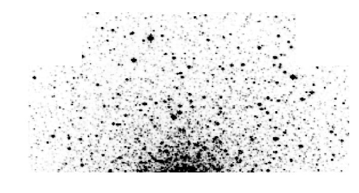
Figure 1: The astrometric reference image of the K2 superstamp of M4. The image is 300 pixels by 150 pixels, or approximately 20′ by 10′, and is displayed with arbitrary z-scale and colors inverted. The white regions in the upper left and right corners are regions that were not included in the superstamp. The core of the cluster is ${\sim}1$′ off of the bottom edge of the image.

M4 was in the field of view of the Kepler telescope during Campaign 2 (running from 2014 Aug 23 to 2014 Nov 10) of the K2 mission (Howell et al., 2014), and continuous observations of a portion of this cluster in the form of a “superstamp” were included in the data downloaded from the observatory. These and other K2 observations of GCs represent, by far, the longest continuous observations of GCs to date, and in the case of M4, the longest continuous observation of what happens to be the closest GC. Additionally, these observations were taken by a space-based observatory designed and built with high-precision photometry as its goal. This is a prime data set for an object of great scientific interest and will likely be the best time series data we have for a GC for a while to come.

Unfortunately, Kepler’s design was not optimized for observing GCs. Its 3$\farcs$98/pixel pixel scale leads to significant blending in the images, particularly close to the core. Fortunately, techniques exist to partially mitigate the effects of the blending, and given the expected richness and value of the derived light curves, the effort to work through these issues is still worthwhile. The present work uses image subtraction (Alard & Lupton, 1998) among other techniques to deal with the blending, and, building off of Wallace et al. (2019a), it is, as far as we are aware, the first general analysis of the K2 observations of a GC. Previous work on these images were limited in scope: Miglio et al. (2016) looked at asteroseismic oscillations in K giants and Kuehn et al. (2017) looked at the RR Lyrae variables, but that has been it so far. The results from these limited searches demonstrate the incredible potential of the M4 K2 superstamp data. This work is focused more on breadth (production of quality light curves and identification of variables) rather than depth (full characterization of individual variable objects) and is only a starting point for analysis of these data. We describe our methods to extract and analyze data from the images in Section 2, and in Section 3 we present the results of our variability search. A discussion is presented in Section 4 and we conclude in Section 5.

2 Method

We present here a detailed description of our data reduction and variable identification pipeline.

2.1 Image Preparation

The images we used are the 16 target pixel files (TPFs) that make up the M4 superstamp from the Mikulski Archive for Space Telescopes. Each is 50 pixels by 50 pixels in dimension. These files had the K2 EPIC ID numbers 200004370 – 200004385. We stitched the TPFs together using k2mosaic (Barentsen, 2016), producing a series of images with dimensions of 150 pixels by 300 pixels, each missing two 50 pixel by 50 pixel notches. These images were ${\sim}$10′ by ${\sim}$20′  on the sky. One of the images is shown in Figure 1. The superstamp is not centered on the cluster, but rather avoids the cluster center, and is focused more on the cluster outskirts on one side of the cluster. A total of 3856 superstamp images are produced, one for each cadence. By mission design, 39 of the images had no data recorded as they took place during resaturation events (major thruster fires used to spin up the reaction wheels) that occurred every 96 cadences and were thus not usable in our analysis.

Our data extraction and reduction pipeline is very similar to that of Soares-Furtado et al. (2017). After assembling the superstamp images, we used the fistar tool from the open-source FITSH software package (Pál 2012) for source detection in preparation for image registration. We used an asymmetric Gaussian model for the point spread function (PSF), a detection threshold of 400 ADUs, the default uplink candidate extraction algorithm, and two symmetric and one general iterations. From this, we generated a list of source positions, fluxes, and PSF shape and width parameters for each detected source. The image with the smallest median PSF full width at half maximum (FWHM) across all the detected sources was chosen as the astrometric reference image. This smallest median FWHM was 1.457 pixels, and the collection of median FWHM values across the images had a mean of 1.503 pixels and a standard deviation of 0.018 pixels. The selected astrometric reference frame image—the 1197th cadence in the campaign, which is shown in Figure 1—also had one of the most symmetric FWHMs of all the images.

The grmatch tool from FITSH was then used to match the detected sources in each image to the selected astrometric reference image and calculate a transformation to register each image to the astrometric reference image. To determine the best parameters for the match, a grid was employed consisting of two different transformation orders (1 and 2) and many different values (170–500) for the maximum number of sources to select from the reference and image source lists (ordered by greatest flux to least) to use for the triangle matching. We ran the grmatch code for each image for all the parameters on this grid. For each image, we adopted the set of parameters which maximized the number of matched objects normalized by the square of the weighted residual, subject to the restriction that at least 100 objects were matched, and that the match was accurate (i.e., the weighted residual reported by grmatch was less than $0.001$ and the reported unity was greater than $0.015$). The FITSH tool fitrans was then used to register each image to the frame of the astrometric reference image using the selected transformation calculated by grmatch.

After registering the images, the next task was to create a photometric reference image to use for image subtraction. For each image, the Euclidean distance (in pixels) of the transformation of a point at the center of the image to the astrometric reference image and the closeness of the PSF size and shape (as measured by the median S, D, and K parameters) of the image to the astrometric reference image were calculated. Cutoff values for the transformation distance and the SDK closeness (respectively 0.0998 pixels and 0.1) were selected such that there were 100 images chosen to be used in the creation of a photometric reference image. The chosen images were taken mostly during the first half of the campaign, which is unsurprising considering the much larger drift in the second half of the campaign. These 100 images were then median combined using ficombine from FITSH to create the master photometric reference image.

2.2 Image Subtraction and Photometry Extraction

FITSH’s ficonv tool was then used to subtract the master photometric reference image from each of the K2 images. A first-order polynomial was fit to the background and also subtracted. A constant discrete convolution kernel with a half-size of 4 pixels was used to match the PSF and flux scale of the reference image to that of each individual K2 image. This unfortunately meant that objects that were within 4 pixels of the edge of the image (a little less than 1% of the image, referred to in this work as “the edge region”) were not included in the image subtraction calculation and objects near to the edge region with parts of their images cut off did not get their photometry calculated. Nine isolated, relatively bright stars across the least crowded portions of the super stamp (left, right, and upper portions) were selected by eye and used to optimize the parameters of the background transformation and the convolution kernel.

What remains after the image subtraction (barring any uncorrected systematics and/or an incorrect background fit) is an image free of any non-variable sources with random scatter about a statistical average of zero. Stars leave behind larger magnitudes of scatter than the source-less background, and saturated stars leave behind visible artifacts. Figure 2 shows the same image as Figure 1 after subtracting the master photometric reference image as described above.

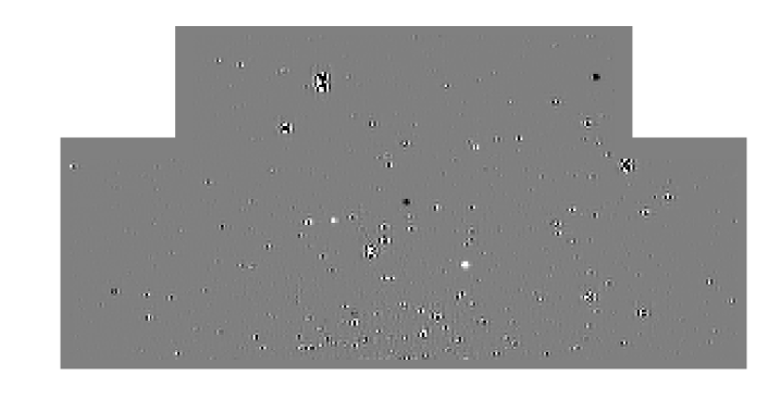
Figure 2: Subtracted image for the image in Figure 1, with arbitrary z-scale of same dynamic range as Figure 1 and no color inversion. The white regions in the upper left and right corners are the same as the white regions in Figure 1, regions that were not included in the superstamp. The RR Lyrae variables are of sufficiently large amplitude to be visible to the naked eye in the subtracted image: the black “holes” in the middle and in the upper right of the image are two RR Lyrae variables, as are the bright spots (i.e., no dark pixels in the star’s image) left and slightly down as well as right and down from the middle hole. Residual noise and saturation artifacts are visible. The 4-pixel border of zero-value pixels filling the edge region, as described in the text, is also present, and can be made out at the bottom of the image.

Extracting photometry from the subtracted images requires a catalog of source positions as well as reference fluxes/magnitudes for each source to properly calibrate the amplitude of the variable signals found in the subtracted images. We used the Gaia first data release (DR1) source catalog (Gaia Collaboration et al. 2016a, b) as both our astrometric (Lindegren et al. 2016) and photometric (van Leeuwen et al. 2017) reference catalog. Our analysis was sufficiently progressed at the release of the Gaia second data release (DR2; Gaia Collaboration et al. 2018) that we chose to stick with the Gaia DR1 data despite DR2’s superior quality. That being said, data from Gaia DR2 were used as part of our analysis (for example, its identification of duplicate DR1 sources).

The Gaia DR1 source catalog is virtually complete at the magnitude range of the main sequence turnoff stars in M4 ($G{\approx}$16–17) and its excellent astrometry allows for precise source position determination and aids in identifying and disentangling close neighbors that are impossible to differentiate in the K2 images. That being said, crowded regions limited Gaia’s completeness in both DR1 and DR2 (e.g., Gaia Collaboration et al. 2016a). Given that these limitations in completeness correlate with crowdedness and that in the most crowded regions of our images, any star missing from our astrometric reference catalog is likely to appear in some other star’s photometric processing aperture, and we proceeded anyway despite the potential completeness issues. Kepler’s and Gaia’s bandpasses are also very comparable, which we found eliminated any need to derive more than an additive conversion from our instrumental magnitudes to Gaia $G$ magnitudes.

From the Gaia DR1 archive, we extracted those sources that fell inside or near to the region of the M4 superstamp and had a $G$ magnitude brighter than 19. This cutoff does not go deep enough to cover all the stars in the cluster, nor does it go deep enough to cover the possible variable stars in the background, many of which may be sufficiently unblended in the images to detect variability. The choice of this magnitude cutoff was based on the photometric performance of Soares-Furtado et al. (2017) and our initial goal to primarily search for transiting exoplanets rather than larger-amplitude variables. The right ascension and declination values obtained for the Gaia DR1 sources were projected onto a pixel-based image coordinate system and then matched using grmatch with the extracted sources of the selected astrometric reference image. The matching, similar to before, was performed over a grid of spatial orders and number of objects to include in the triangle matching. The best transformation was then chosen as the match with at least 100 matched objects, weighted residual less than 0.001, and unitarity greater than 0.015 that had the largest number of matched objects normalized by the square of the weighted residual. We then transformed the coordinates of the Gaia DR1 sources to the astrometric reference image’s frame using grmatch based on the transformation calculated above. After removing those sources with transformed coordinates that fell outside the astrometric reference image, there were 5914 sources. We refer to this as our source position catalog.

The next step was to calculate the photometry for each of the 5914 sources from the subtracted images. This required first deriving a conversion from the the $G$ magnitudes of the photometric reference catalog to the instrumental magnitudes of the K2 images. To accomplish this, we first used the FITSH tool fiphot to obtain photometry from the master photometric reference image for a set of circular apertures, with 15 apertures ranging from 1.15 to 2.55 pixels. These radii were selected to obtain a good measure of how changing the aperture size affected the amount of flux measured for a given source over a range relevant to where the bulk of the flux falls in the PSF (the median FWHM of the PSF across the images was ${\sim}$1.5 pixels, with the range 1.45–1.55 pixels covering nearly all the median PSF widths). The apertures were centered at each of the positions of the 1024 objects that had been directly matched between the Gaia DR1 source catalog and the astrometric reference image. (Since fiphot had found only 1073 sources directly from the images, probably due to inability to disentangle highly blended sources, that is why there were far fewer matched sources than the total available from just the Gaia DR1 source catalog.) For this calculation, the sky was subtracted based on the mode of pixel values in an annulus with inner radius of 17 pixels and outer radius of 30 pixels. A radius of 3 pixels around any source in the set of 1024 matched sources was excluded from this background calculation, and the pixel values were sigma-clipped (3$\sigma$, two iterations) prior to the calculation.

After performing this reconnaissance photometry, we determined a transform from Gaia $G$ to Kepler instrumental magnitudes. As mentioned previously, we found that an additive transform was all that was needed for this conversion, likely because of the very similar bandpasses of the two instruments. Since there is significant blending of the sources in the K2 images, we first selected out those K2 sources for which we thought there were negligible contributions from neighbors. Several unblended sources, as well as a few unsaturated bright sources for which any blending from neighbors would be small, were selected from the astrometric reference image by eye and were verified to be negligibly blended by using the Gaia DR1 source catalog. After this, sources with instrumental magnitudes in a narrow range around the transformed $G$ magnitudes (and thus presumably negligibly blended on the images) were selected and then fit to determine a more precise value for the additive constant. For all this, we used a 2.5-pixel radius aperture to calculate the instrumental magnitudes. Next, we determined the effect that changing the aperture size had on this conversion factor. For the brightest unblended and unsaturated stars, we normalized the fluxes calculated over a range of aperture sizes to the flux in the 2.5-pixel aperture and then determined the median normalized flux for each aperture size across the selected stars. We then fit the integral of a Gaussian function to the median normalized fluxes to determine a conversion from the flux at a given aperture size to that of the 2.5-pixel aperture.

We then ran aperture photometry on the master photometric reference image for all the positions in the astrometric source catalog. As before, the sky background was calculated as the mode of pixels values in an annulus with inner radius of 17 pixels and outer radius of 30 pixels, with the same sigma clipping and source exclusion as before. The background was then subtracted. We performed the photometry calculation with apertures 1.5, 1.75, 2.0, 2.25, 2.5, 2.75, and 3.0 pixels in radius. Then, using the G magnitudes from the photometric reference catalog, we substituted the reference fluxes for each object with the values determined from the converted G magnitudes, additionally modified based on the aperture size. This provided reasonably accurate and unblended reference fluxes for each of the objects.

We then calculated the image subtraction photometry using fiphot and the derived reference fluxes. The sky background, having been previously subtracted when the subtracted images were created, was not fit in this step. We also used the same convolution kernels calculated for the creation of the subtracted images. At this point, Kepler BJDs (KBJDs; BJD$-2454833.0$) were assigned to each cadence for each object. Each of the original 16 TPFs was assigned only a single KBJD for each cadence, calculated along the center of the TPF. We assigned to each object the KBJDs from the TPF image in which it was found.

After the photometry calculation from the image subtraction, we obtained light curves for 4601 objects. The reason for the reduction from the original 5914 we were calculating photometry for was that some objects were excessively blended with much brighter neighbors and were unable to have photometry measured, and that some of the objects fell in or excessively overlapped with the excluded edge region. The brightest stars (for cluster members, this corresponds to many of the giant stars) were saturated. We did not perform any special treatment of saturated stars, though because they were so bright the largest apertures employed in our processing (3 pixel radius) were used. Additionally, there was one previously know RR Lyrae variable, V27 of Clement et al. (2001), that was not a Gaia DR1 source and thus did not get a light curve through the above method. We separately extracted a light curve for this star following the procedure described above and based on the transformed Gaia DR2 position for this object. The light curve for V27 did not undergo any of the following post-processing procedures since large-amplitude variables were not served well by the roll decorrelation, described in Section 2.3. Including V27, we produced 4602 light curves in total. The light curves at this stage are what we refer to as the “raw light curves” throughout the rest of this work. All of our raw and processed light curves are published and publicly available at Wallace et al. (2019b).

2.3 Photometry Post-processing

The roll of the telescope during the K2 mission introduced systematic variations to the brightness of objects as they moved across the detector (Howell et al., 2014). This is due to differences in pixel sensitivity unaccounted for in the K2 data reduction. These brightness variations are correlated with the object position on the detector, and are not fully corrected by the image subtraction photometry. The remaining systematic variations can be decreased by performing a decorrelation of flux variations against object position with a procedure based on Vanderburg & Johnson (2014) and Vanderburg et al. (2016). We divided the light curves, normalized to their median values, into the same eight time chunks as Vanderburg et al. (2016) did for Campaign 2 (A. Vanderburg, private communication). To determine the drift position of each object, the positions in the source position catalog were transformed for each cadence using the inverse of the transformation originally used to register each cadence’s image to the astrometric reference frame. Since the drift of objects across the detector was primarily in one direction, for each object we used a principal components analysis (PCA) to determine this primary direction of drift. The object positions for each cadence were transformed to the axes defined by the PCA and then a fifth-order polynomial was fit to the positions. Each object’s drift’s arc length along the polynomial at each cadence was calculated and stored for later decorrelation.

For each time chunk, we iterated over fitting long-term trends with a B-spline fit and decorrelating against the roll. For the B-spline, we had breakpoints set nominally every 1.5 days. The 1.5-day breakpoint spacing was adjusted to allow for knots to be distributed evenly across the time chunk. Also, where possible, 0.75 days from adjacent time chunks were included to improve the smoothness and accuracy of the spline fit across time-chunk boundaries. We then excluded 3-$\sigma$ outliers to the B-spline fit, refit the spline, and repeated this until no outliers remained to be removed. The median-normalized light curve was then divided by the spline fit. The spline fit is not ever reintroduced into our light curves, so smoothly varying signals with timescales longer than the 1.5-day knot placement are likely to either be altered or removed. Objects with such signals are best studied from our data using the raw light curves.

After this, the fluxes of each chunk of the light curve were binned into 15 bins in arclength. 3-$\sigma$ in flux outliers were excluded in each bin, and then a linear interpolation was made using the mean flux values of each non-empty bin. In cases where bins had only a single point, an interpolation between adjacent bins was made. If there was a single point in the last bin (usually corresponding to outliers in the pointing), no fit was made for that point. The light curve was then divided by this interpolation. This process of fitting a spline to the longer trends and decorrelating against position was repeated eight times or until convergence, whichever came first. We selected eight to be the maximum number of times because we found those light curves that required more than eight iterations were usually oscillating between two close fits to the data that were not quite close enough to be counted as converging. If less than 10 points were in a time chunk, the decorrelation against drift position was not performed.

We then used the trend filtering algorithm (TFA; Kovács et al. 2005) as implemented in VARTOOLS (Hartman & Bakos 2016) to clean up systematics common across the light curves. For each aperture, 250 light curves with at least 97% of the maximum number of light curves points were selected from uniform bins of source position and magnitude to be used as the trend light curves. For light curves with less than 2500 points, a subset of the selected 250 trend light curves was used in the detrending, with the number of selected trend light curves being close to but less than 10% the number of light curve points. Since the KBJDs for a given observation differed slightly depending on which TPF an object was located (see Section 2.2) and common instrumental effects were likely correlated based on actual observation time than KBJD, detrending was performed based on cadence number rather than KBJD. Light curves from stars that were known to be RR Lyrae variables or saturated were not included as potential trend light curves. All light curves were then detrended against the trend light curves for the given aperture size with trend light curves excluded from the detrending if they were closer than 6 pixels, which is ${\sim}$4 FWHMs. The light curves that resulted were the ones used in our variability search and are referred to in this work as “final light curves.” Figure 3 shows the root-mean-square (RMS) scatter of the sigma-clipped (3-$\sigma$ clipping, iterated three times) final light curves for those objects included in our variability search. Owing to significant outlier points in our final light curves, outlier removal was necessary for our subsequent period search. These outliers seem to be due to still-uncorrected systematics, the worst of which occurred when the telescope changed its roll direction about halfway through the campaign.

The photometric performance displayed in Figure 3 shows that our sigma-clipped light curves are able to reach millimagnitude RMS scatter down to $G{\approx}15$, and 0.01 mag RMS scatter down to $G{\approx}18$. There is a large envelope of points with significantly larger scatter than is typical for objects of their magnitude. Some of these are variable stars, while the rest have excessive scatter due to the amount of blending present in the images or also possibly due to breakdowns of the photometric processing for individual objects. We also note that our saturated giant/bright foreground stars do not have significantly larger scatter than, e.g., our HB stars at $G{\approx}13$. The point at $G{\approx}9.5$ is a star that is an intrinsic variable, hence the larger scatter. The clump of points with high RMS scatter at $G{\approx}13$ are the RR Lyrae variables.

The solid line in Figure 3 shows our expected RMS performance based on source Poisson noise and the background sky flux as seen in our photometric reference image and the dotted line shows the same expected RMS performance reduced by a factor of three. We have not entirely determined the reasons for our photometric performance to fall as far below our expected performance as it does, but it is perhaps attributable to some combination of an incorrect gain value, an incorrect sky background characterization, an incorrect magnitude zero-point determination, or outliers being excessively clipped due to large, non-Gaussian errors. We note that our roll decorrelation and TFA calculations have some free parameters, but this at most could account for only a few percent decrease of the scatter relative to the expected.

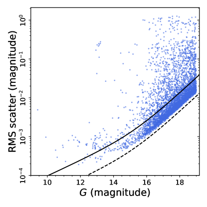
Figure 3: RMS scatter as a function of Gaia DR1 $G$ magnitude for our final light curves. The RMS is calculated from our magnitude light curves, which have been sigma clipped with 3-$\sigma$ clipping iterated 3 times. All of our final 4554 objects under consideration except V27 are plotted here; V27’s light curve did not undergo the same processing as those of the other objects, see text for details. The solid line shows a calculation of our expected RMS scatter and the dashed line shows that same calculation reduced by a factor of 3; see text for a discussion. The collection of objects with excessive RMS values at $G{\approx}13$ are the RR Lyrae variables, though we note that our light curve processing pipeline impacted the amplitudes of large-amplitude variables.

2.4 Skipped Images

Now that the photometric processing pipeline has been explained, sufficient context is available to discuss why certain cadences were not used in our analysis. In what follows, the cadence numbering starts at 1 for the first cadence in the campaign (which corresponds to the Kepler long cadence number of 95497). Of the 3856 cadences in Campaign 2, 39 were blank due to resat events, an additional 6 were blank due to other reasons (cadences 216–218 and 2856–2858), 12 were excluded due to our noticing excessive telescope slew during the exposure (cadences 50, 191, 202, 203, 205–207, 209, 383, 863, 1535, and 1823), 68 were excluded due to being excessive pointing outliers (1–49, 51–57, 192–201, 204, and 727), one was excluded due to a hot pixel column we noticed (208), and six were excluded due a majority of the light curves having large outliers (at least 50% off) in flux measurements relative to the median flux value across the whole light curve (2150, 2151, and 2153–2156)—these all occurred around the point in the observations when the telescope roll direction switched. For the pointing outliers, cadences 1–49 were all pointed in a locus several pixels away from the main group of pointings, and this was an insufficient number to perform our roll decorrelation just on these points; cadences 192–201 and 204 were similarly pointed in a different locus several pixels away from the main; cadences 51–57 were pointed in a locus close to the main locus of pointing but not close to the pointings of its time chunk; and similarly the pointing of cadence 727 was quite disparate from any in its time chunk. This is a total of 132 cadences that were entirely removed from or not available for our consideration, leaving 3724 (96.6%) of the cadences for the final analysis. We note that most of the these cadences were removed from both our raw and final light curves, but that cadences 1–49 are still present in the raw light curves.

2.5 Removal of Objects

We removed from consideration objects with light curves with less than 800 points (out of a maximum number of 3724 for the final light curves). There were 32 such objects in total, leaving 4570 objects. These removed objects tended to be highly blended with a much brighter object, and this led to many light curve points’ calculations failing. In practice, we found that such light curves were not productive to search for variability. The selected cutoff of 800 was rather conservative and still permitted other relatively sparse and blended light curves that were not useful, so the removal of these objects is not likely to remove anything that might be detected as a variable.

2.6 Additional Data Used for Analysis

We used the Gaia DR2 gaia_dr2.dr1_neighbourhood crossmatch catalog to inform us which of the examined Gaia DR1 sources were duplicates. There were 16 DR2 sources matched to two entries in the DR1 source catalog. So that the photometric aperture used corresponded as closely as possible to the DR2 source position, in each case we kept whichever of the two DR1 sources was closest in position to the corresponding DR2 source. This also happened to correspond in each case with the DR1 source with the best “RANK” value—a calibrated measure of how close a DR1 source is to a DR2 source in both position and magnitude—between the two DR1 sources. We removed the 16 extraneous DR1 sources from the analysis and were left with a final set of 4554 objects with usable light curves. Information on these objects and their light curves is presented in Table 1.

Table 1: Stars Examined

ID	Gaia ID	R.A.	decl.	$G$	$G_{\mathrm{BP}}$	$G_{\mathrm{RP}}$	No. Pnts.	RMS	Mem. Prob.
		(hh:mm:ss)	(dd:mm:ss)	(mag)	(mag)	(mag)		(mmag)
V6	DR2 6045478696063803648	16:23:25.76	$-$26:26:16.7	13.25	13.68	12.63	3773	120.82	1.000
V7	DR2 6045478391137284224	16:23:25.92	$-$26:27:42.3	13.28	13.80	12.61	3762	285.46	1.000
V8	DR2 6045477910100852736	16:23:26.12	$-$26:29:42.0	13.23	13.64	12.49	3773	255.69	1.000
V9	DR2 6045477910100361600	16:23:26.76	$-$26:29:48.4	13.10	13.59	12.44	3773	256.94	1.000
V10	DR2 6045478322417726848	16:23:29.17	$-$26:28:54.7	13.19	13.64	12.53	3087	155.06	1.000
…

Note. — There is no W1873 in this table. The identifiers beginning with “W” are sequential otherwise. Light curves for all of these sources are available at Wallace et al. (2019b). Table 1 is published in its entirety at Princeton University’s DataSpace and can be found in the object_information.txt file at the URL http://arks.princeton.edu/ark:/88435/dsp01h415pd368. A portion is shown here for guidance regarding its form and content.

As part of our analysis, knowledge of the cluster membership of each of the stars was necessary. We used the membership catalog previously created by Wallace (2018b) and available at Wallace (2018a) or on GitHub. This catalog fitted a two-component Gaussian mixture model to Gaia DR2 proper motions (Lindegren et al., 2018) to calculate a membership probability for all Gaia DR2 sources with reported proper motions. A very large majority of the calculated membership probabilities were ${<1}$% or ${>99}$%, essentially allowing the catalog to function as a binary classification in all but a few cases. Of the 4554 objects with usable light curves, 4469 of them—98.1%—were matched (again, using the gaia_dr2.dr1_neighbourhood crossmatch catalog) to a single DR2 source with reported proper motions and thus were able to be assigned a cluster membership probability. Of the remaining 85 objects, 74 were matched to DR2 sources that lacked reported proper motions, 6 were matched to more than one DR2 source, and 5 were not matched to any DR2 sources. Membership probabilities for these 85 objects were not calculated. Of the 4469 objects with reported proper motions, 3784 of them had calculated membership probabilities of ${\geq}99$%.

2.7 Search for Variability

We used three algorithms for finding periodic signals in our data: the Generalized Lomb-Scargle (GLS; Lomb, 1976; Scargle, 1982; Zechmeister & Kürster, 2009), phase dispersion minimization (PDM; Stellingwerf, 1978),  and box-fitting least squares (BLS; Kovács et al., 2002) algorithms. The astrobase (Bhatti et al., 2017) implementations of these algorithms were used. With the amount of signal blending in the data, we incorporated a blend search with the period search. It is worth noting that this blend search incorporated only data available from the section of the superstamp we examined. Any blending or systematics due to objects that were in the edge region of the superstamp or beyond could not be readily identified. Additionally, with the amount of systematic noise remaining in the data, it was necessary for us to employ a custom and period-dependent SNR threshold, determined from our examination of the data. The code written to perform both of these tasks, simple_deblend, is available at Wallace & Hoffman (2019) or on GitHub.

The basic framework of the algorithm used by simple_deblend is as follows. For a given period search method (GLS, PDM, BLS) and star, the code:

• Determines the best period based on the period search

• Checks the periodogram SNR of this period against the threshold; if below the threshold, then quits the period search

• Phase-folds neighbor light curves at the given period and figures out which of all the objects has the highest flux amplitude of variability

• Records the star as the source of that variability if the star has the highest flux amplitude of variability

• Fits out the found period using a Fourier series fit to the data, then repeats

This is repeated for the desired number of periods—three for our analysis—or until no more robust signals are found.

As a more detailed description, for a given period search method and star, the code runs the astrobase implementation of the period search algorithm. In each search, working in magnitudes (and not fluxes), the minimum period searched was 0.06 days and the maximum period search was 78 days for GLS and PDM—about as long as the maximum duration of the final light curves—or, for BLS, half the observation duration of the light curve. A frequency grid for the search was selected automatically with the autofreq parameter set to true. For GLS and PDM, this produced a frequency grid with frequency spacing $\Delta f=1/(5\times L)$, with $L$ being the duration of the observations. For BLS, this produced a frequency grid with $\Delta f=0.25\times q_{\mathrm{min}}/L$, with $q_{\mathrm{min}}$ being the minimum transit duration in units of fractional phase. This was set to 0.02 and the maximum transit duration was set to 0.55. For BLS, the number of phase bins also needed to be set, and was set to 200.

After running a period search, the resultant periodogram was median filtered to correct for trends that were presumably due to non-white noise. For each point in the periodogram, either 40 (for GLS and PDM) or 100 (for BLS; larger due to its smaller $\Delta f$) of the periodogram values on each side, outside of an exclusion area that was equal to $4/L$ on each side, were collected and were 3-$\sigma$ sigma clipped before calculating their median, which was then subtracted to produce the filtered periodogram. For PDM, which has periodogram values of one for frequencies with no power, the filtered periodogram values had one added back on. The peak with the highest power was then found, and the robustness of this peak was determined using an SNR calculation on the median-filtered periodogram values. The noise for the ratio was calculated using the standard deviation $\sigma_{\mathrm{per}}$ of nearby periodogram values collected in the exact same way as described above for determining the median filter. The SNR value was then simply the ratio of the periodogram value $p$ with this standard deviation, $p/\sigma_{\mathrm{per}}$ or, for PDM, $(1-p)/\sigma_{\mathrm{per}}$. Appropriate thresholds for this SNR were determined as a function of period by comparing the SNR values for objects and periods with previously determined variability and (for BLS) injected transits with the rest of the detected periods. This and the selected thresholds are show in Figure 4. If the SNR did not exceed the threshold, the period is marked as not robust and the periods search for this object was done.

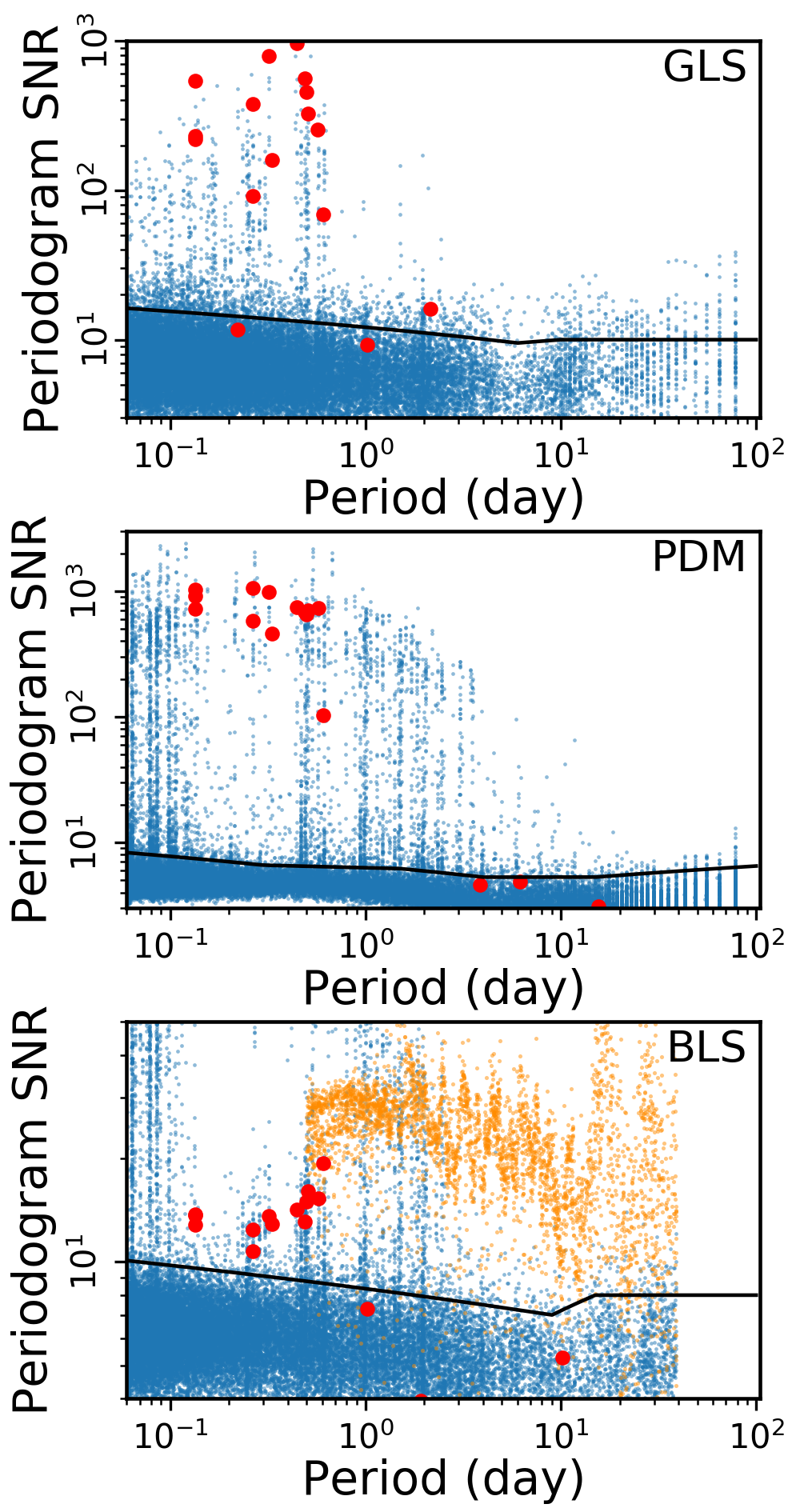
Figure 4: Thresholds for the periodogram SNR for the three period search methods. The corresponding period search method is shown in the upper right of each panel. The blue points show the values calculated from the best eight periods found for each object. For BLS, the orange dots show the values for light curves with injected transits from transiting objects with radii between 0.3–3.5 R_J. For all panels, the red dots show the periodogram SNR values for objects and periods we identified as being variables during some initial reconnaissance of the data. Not all variables are identified by all the methods, so there are red dots missing between the panels. The thresholds used in our analysis are plotted with a black line in each panel.

If the period was determined to be robust using the SNR threshold described, the next step was to check for blends. The light curve was fit with a seven-harmonic Fourier series, which was then evaluated at 200 evenly spaced points. A flux amplitude was then calculated using the minimum and maximum of these Fourier series evaluations, converted from magnitudes. Subsequently, all neighbors within 12 pixels had their flux amplitudes at the same period determined in the same fashion. The choice of 12 pixels was determined by choosing two RR Lyrae variables and looking at all the light curves for surrounding objects to see how far their influence extended. If the object was determined to have the largest flux amplitude, then the period was considered a valid detection, and an 11-harmonic Fourier series fit at the period was subtracted, except for the offset term, from the light curve for subsequent period determination.

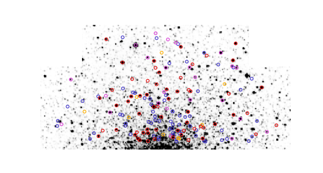
Figure 5: Locations in the superstamp images of our detected variables and suspected variables. This is the same image as in Figure 1. Red circles mark the positions of the cluster-member variables, magenta circles the positions of variables that are not cluster members or with ambiguous cluster membership, gold circles the positions of variables that are indistinguishably blended (only one circle per set of blended stars), and blue circles the positions of suspected variables irrespective of cluster membership. Light curves were not obtained for stars in the edges of the images and so no variables were found in those areas; see text for details.

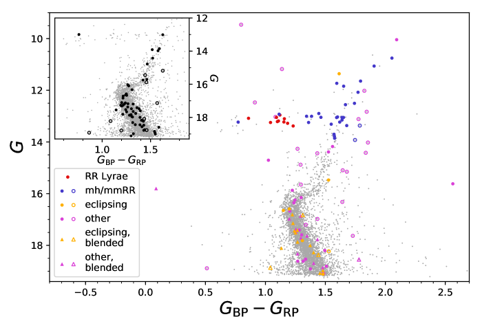
Figure 6: Color-magnitude diagram for the stars we obtained light curves for, with variables marked. The photometric data are taken from Gaia DR2 (Riello et al., 2018). Of the 4554 objects we obtained light curves for, 11 objects did not have any DR2 data, and 92 objects were missing $G_{\mathrm{BP}}$ and/or $G_{\mathrm{RP}}$ data and are not included here. None of the variables or suspected variables were missing these data. The gray points show the data for all the objects. Red points show the data for the RR Lyrae variables, blue points the data for those objects classified as multiharmonic or millimagnitude RR Lyrae variables, gold points the data for objects classified as some type of eclipsing binary (EA, EB, or EW), and magenta points the data for other types of variables. Those variables that are cluster members are marked with closed symbols and those that are not cluster members or have ambiguous cluster membership are marked with open symbols. Circle symbols are those for which one object is identified as the variable, while triangle symbols mark variables that are indistinguishably blended. The inset shows the same data, but with the suspected variables marked in black, and with the same open/closed symbol membership convention as the main panel. Note the differing scales between the main panel and the inset.

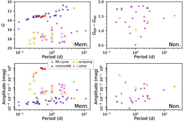
Figure 7: Relationships of photometric properties and variability amplitudes with variability periods. The left two panels are for variables that are cluster members and the right two are for variables that are not cluster members or have ambiguous cluster membership (indicated by, respectively, “Mem.” and “Non.” in the lower right corners of each panel). The top-left panel shows $G$ versus period and the top-right panel shows $G_{\mathrm{BP}}-G_{\mathrm{RP}}$ versus period. Both the bottom-left and bottom-right panels show variability amplitude (see Section 2.8) versus period, with amplitude converted to a positive value for those few cases with negative amplitudes as we have defined it. The x-axis scales are the same for panels in the same column, and the y-axis scales for the bottom-left and bottom-right panels are the same. The legend of the bottom-left panel applies to all panels: red diamonds are RR Lyrae variables, blue stars are multiharmonic and mmRR variables, gold X’s are eclipsing variables, and magenta squares are all other variables. Solid symbols are for variables identified to single objects and hollow symbols are for variables indistinguishably blended with others. In the x-axis labels, “d” stands for “day.” The period–luminosity relation of the RR Lyrae variables is seen, and the multiharmonic variables also appear to continue this relation to longer and shorter periods.

We noticed two cases where known low-amplitude variables—specifically, the millimagnitude RR Lyrae (mmRR) variables of Wallace et al. (2019a)—were marked as blends. This was because their periods were ${\sim}\text@frac{2}{3}$ that of some large-amplitude-variable neighbors. Although folding these neighbors’ light curves on the mmRR variability period did not produce the ideal folding for these neighbors’ variability, the folded neighbor light curves still had a large enough amplitude to be larger than the mmRRs’ ${\sim}$mmag variability. Because of this, if the object was determined as not having the largest flux amplitude, then the neighbor with the largest flux amplitude at the given period was checked to make sure that period corresponded to a “real” period of the object. This was determined by running the given period search method on the neighbor’s light curve and checking whether the found period matched any of the neighbor’s top 8 periods. If the period matched any of the neighbor’s top 8 found periods, then the period was marked as a blend and, as for the valid period, the light curve with an 11-harmonic Fourier series fit removed (except for the offset term) was then used for a subsequent period search. This recursed until either a valid period was found, a period was determined to not be sufficiently robust, or, in the case of sequential finds of blending, a recursion limit was hit. This recursion limit was set to be 4 for GLS and PDM and 3 for BLS. Additionally, if a particular object and period’s flux amplitude was not the greatest but was greater than 90% the maximum flux amplitude of its highest-amplitude neighbor, it was marked as a possible source of the variability.

The 1310 objects thus determined to have robust periods were then searched by eye for classification and to weed out false positives. For this by-eye evaluation, we used the checkplot submodule of astrobase. After variables and suspected variables were identified, those with similar periods were checked against each other to look for blends by evaluating the similar shapes and phasing of the variability. In many cases, nearby stars were blended with each other, but in some cases the identified blends were quite spatially disparate and may have arisen from some effect of our photometric processing. Appendix A provides specific details on these manually determined blends. We had 161 variables or suspected variables remaining after this manual step.

The periodogram SNR selection criterion as we implemented it was not robust to detect objects with strong variability at a variety of fairly close periods, such as giant stars with solar-like oscillations. This is owing to the calculated noise being artificially high from the variability at these other periods. In fact, in Figure 4, most of the red points that fall below to the thresholds belong to such asteroseismically active objects. For simplicity and given the breadth-focused nature of this work, we did not make a special search for such variability in those stars for which we may have had a priori reasons for suspecting such variability, and we know our accounting of such variables in this work is incomplete. Readers interested in such variability are encouraged to download the light curves and perform their own searches.

2.8 Amplitude, Epoch, and Final Period and Period Uncertainty Determination

For each object determined to be a variable or a suspected variable, a final period search was made using one of our three period search methods with a fine frequency grid ($\Delta f=10^{-6}$) in a restricted region of frequencies. These frequencies corresponded to possible periods based on the observation duration and the period originally detected in our variability search. The period with the strongest power in this finer search was selected as the final period for the object. For objects with narrow eclipses, a trapezoid model was instead fitted to determine the period, amplitude (trapezoid depth; quoted as a negative number in the case of inverse transits), epoch (center point of transit), and period uncertainty. For all other objects, the amplitude and epoch were derived from a multiharmonic fit to the phase-folded light curve, with amplitude being derived from the difference between the minimum and maximum values of the fit and epoch being the KBJD of the minimum of the fit. The number of harmonics used varied from object to object, with the most being 11 (for the RRABs) and the least being 1, and most objects having between 1–5 harmonics for their fits. Epochs were always adjusted to be within one period of the KBJD of the earliest observations of our final light curves, KBJD $=$ 2060.284181. Period uncertainties were derived from bootstrap resampling, with 100 resamplings, and with the fine-grid search described above being performed on each resampling and the quoted uncertainty being the difference between the 15.865 and 84.135 percentiles of the calculated periods. Such values are more of a confidence interval than a formal uncertainty, but we still quote them as our period uncertainties. Uncertainties on epochs and amplitudes were not determined.

3 Variability Search Results

The presentation of the results is organized based on the cluster membership probability of the star, whether it is a horizontal branch (HB) star, and whether a given variability signal is certain, suspected, or indeterminably blended. As far as possible, we adopt the same variability classification scheme, including abbreviations, as used in the General Catalog of Variable Stars (GCVS), March 2017 edition (Samus et al., 2017), with additional designations to describe variability not described in this classification scheme. Other than W1189, W3756, and the variables in the Clement et al. (2001) catalog, none of the variables or suspected variables presented here are cross-listed in the GCVS. As part of our breadth versus depth approach, most of our variables go unclassified.

Table 2: Results for Variables from Clement et al. (2001) and Stetson et al. (2014)

ID	R.A.	decl.	$G$	Period	Per. Uncertainty	Amplitude	Epoch	Type
	(hh:mm:ss)	(dd:mm:ss)	(mag)	(day)	(10-5 day)	(mag)	(KBJD)
V6	16:23:25.76	$-$26:26:16.7	13.25	0.320500	0.6	0.33	2060.58	RRC
V7	16:23:25.92	$-$26:27:42.3	13.28	0.498787	0.7	0.99	2060.55	RRAB
V8	16:23:26.12	$-$26:29:42.0	13.23	0.50822	1	0.87	2060.45	RRAB
V9	16:23:26.76	$-$26:29:48.4	13.10	0.57192	2	0.87	2060.36	RRAB
V10	16:23:29.17	$-$26:28:54.7	13.19	0.490723	0.4	0.87	2060.70	RRAB
V13	16:23:30.88	$-$26:27:04.4	10.04	${\sim}$20–30	…	${\sim}$0.1	…	SR
V15	16:23:31.93	$-$26:24:18.5	13.38	0.443795	0.4	1.03	2060.57	RRAB
V19	16:23:35.02	$-$26:25:36.8	13.21	0.467809	0.4	0.99	2060.38	RRAB
V27	16:23:43.14	$-$26:27:16.7	12.96	0.612027	0.8	0.76	2060.74	RRAB
V29	16:23:58.22	$-$26:21:35.4	13.05	0.52250	1	0.75	2060.69	RRAB
V61	16:23:29.72	$-$26:29:50.7	13.08	0.265293	0.7	0.13	2060.49	RRC
V66	16:23:25.53	$-$26:29:12.1	16.59	0.269889	0.4	0.22	2060.29	EW
SC3	16:23:35.57	$-$26:27:08.3	16.32	${\sim}$19	…	${\sim}$0.1	…	?
SC4	16:23:44.77	$-$26:24:29.4	14.88	0.43863	2	0.033	2060.62	?
SC5	16:23:34.58	$-$26:25:41.6	18.73	…	…	…	…	…

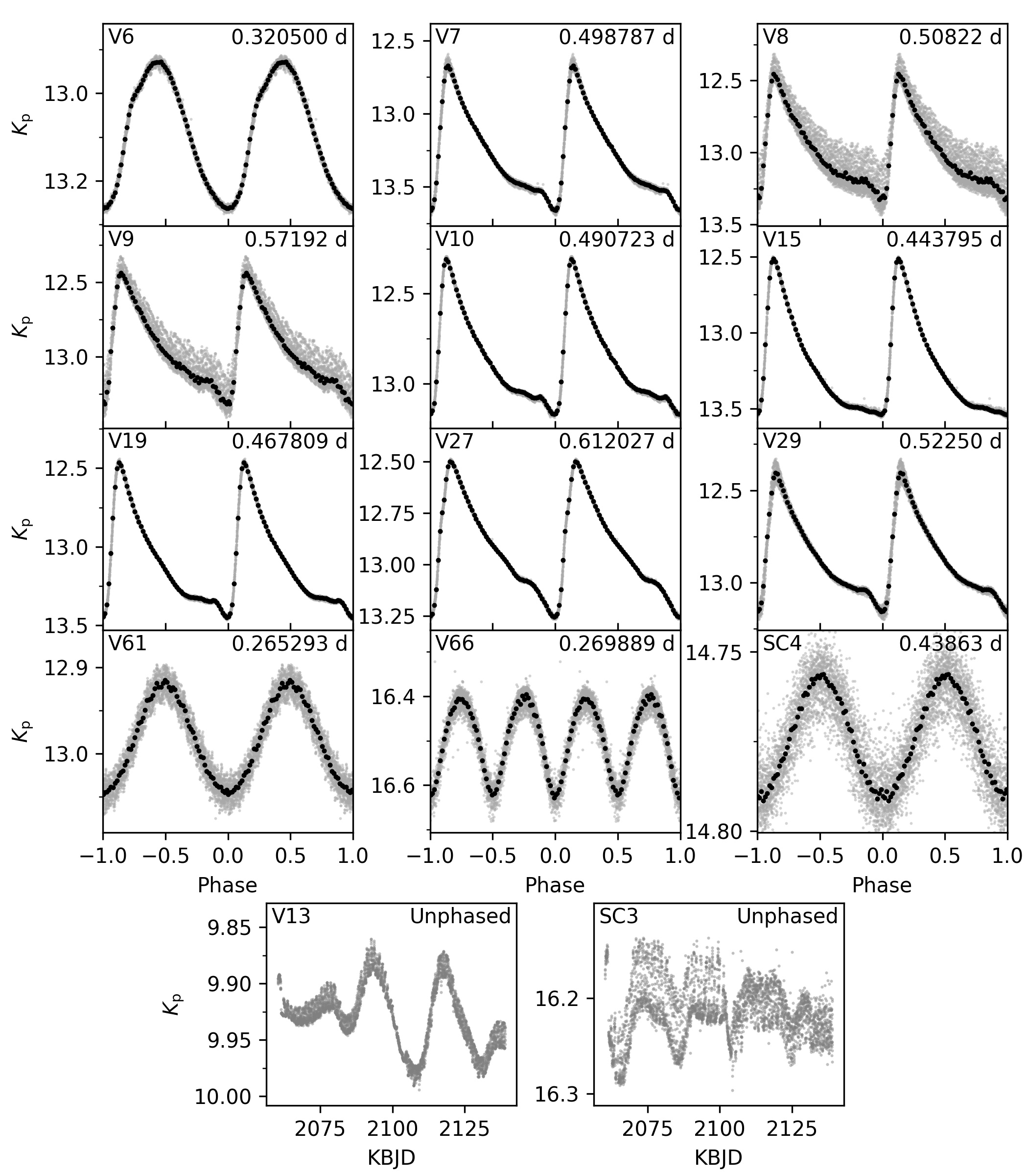
Figure 8: Light curves for 14 previously identified variables from Clement et al. (2001), June 2016 edition, and Stetson et al. (2014) that were in the K2 superstamp and for which we have light curves. Phase-folded light curves are shown in the top 12 panels, while the bottom two light curves show unphased light curves for V13 and SC3. The top left of each panel shows the identifier for the associated star, and the top right shows the period (or “Unphased” for V13 and SC3) at which the light curve is folded, with “d” standing for “day.” Gray points show the individual magnitude measurements, while the black points are binned-median values. For all light curves except that of SC4, the raw light curve output from our image subtraction is used. SC4, along with almost all the other light curves presented in this work, has the additional roll decorrelation and TFA post-processing as described in Section 2.3.

3.1 Summary Figures

We first present some figures showing general results from the variability search. Figure 5 shows the positions of the variables in the superstamp images, differentiated by cluster members, nonmembers, blended variables, and suspected variables. Figure 6 shows a color-magnitude diagram (CMD) for the examined stars, with the identified variables and suspected variables marked. The HB is visible at $G{\approx}13$ and $0.5\lesssim G_{\mathrm{BP}}-G_{\mathrm{RP}}\lesssim 1.6$, and the main sequence turnoff is visible at $G{\approx}16.5$ and $G_{\mathrm{BP}}-G_{\mathrm{RP}}{\approx}1.2$. We note two stars that are proper motion cluster members and are well off the expected photometric track. The magenta triangle at $G_{\mathrm{BP}}-G_{\mathrm{RP}}{\approx}0.0$ is W1136 and is blended with several other stars (Gaia DR2 source catalog has four other stars within 5″). However, the Gaia DR2 data does not indicate any potential errors in the photometric measurements: its $G_{\mathrm{BP}}$ flux error over mean flux is $3.7\times 10^{-3}$ and $G_{\mathrm{RP}}$ flux error over mean flux is $2.2\times 10^{-3}$ and phot_bp_rp_excess_factor of 1.24. The magenta circle at $G_{\mathrm{BP}}-G_{\mathrm{RP}}{\approx}2.5$ is W4490 and has no Gaia DR2 sources within 5″. Its $G_{\mathrm{BP}}$ flux error over mean flux is $7.6\times 10^{-3}$ and $G_{\mathrm{RP}}$ flux error over mean flux is $2.0\times 10^{-3}$, while the phot_bp_rp_excess_factor is 1.46. However, W4490 is a unique object (likely an X-ray binary) that we discuss further in Section 3.4. Figure 7 shows photometric data and variability amplitudes versus periods for all of the variables. Of particular note is the period-luminosity relationship seen in the upper-left panel for objects with multiharmonic variability that mirrors that seen for RR Lyrae variables. This will be further discussed in Section 3.4.

3.2 Clement et al. (2001) and Stetson et al. (2014) Variables

This subsection focuses exclusively on the previously known variables found in the catalog of Clement et al. (2001), June 2016 edition, with additions from Stetson et al. (2014). This does not include the other previously known variables of W1189, reported as a delta Scuti (DSCUT) variable by Yao & Tong (1989), W3756, reported as a gamma Doradus (GDOR) variable by Yao et al. (2006a), or the asteroseismic giant stars of Miglio et al. (2016); these are discussed later. We also note that none of the new variables of Safonova et al. (2016), which are not in the Clement et al. catalog, fell on the superstamp. A summary of the results for sources not marked “CST” (constant) in the Clement et al. catalog is found in Table 2, and the associated light curves are found in Figure 8. There are 12 variables from the Clement et al. (2001) and two from Stetson et al. (2014) that fell into our observable region. The 12 Clement et al. variables were first discovered by Leavitt & Pickering (1904) (V6–V10, V15, V19, V27, and V29), Yao et al. (1988) (V61), and Kaluzny et al. (1997) (V66; called V47 in the discovery work). Given the variability amplitudes for the Clement et al. variables, for Figure 8 the raw light curves were used, as our implementation of the Vanderburg-style roll decorrelation did not perform well for objects with large-amplitude variability at timescales shorter than our spline fit. As a note, we count 17 Clement et al. variables in the edge regions for which we did not obtain image subtraction photometry. We mention this here to show that there is still more that can be done with the superstamp data than what is presented in this work. For example, simple aperture photometry could be used on those stars in the less crowded portions of the edge region.

V6, V7, V8, V9, V10, V15, V19, V27, V29, and V61 are all RR Lyrae variables. V6 and V61 are RRCs, while the others are all RRABs. Our period-search method did not detect any significant variability at periods other than (sub)harmonics of the main period, but we wish to stress that our method was focused more on deblending and primary period finding than on a detailed analysis of small-scale variability in these RR Lyrae variables. Kuehn et al. (2017) performed such an analysis for the RR Lyrae variables in the M4 K2 superstamp.

V8, V9, and V61 are in fairly close proximity to each other and to a few other HB stars. In particular, V8 and V9 are blended and we observed a beating effect between their two periods that created the increased scatter of their light curves seen in Figure 8. We did not correct for the blending between these two stars, though in principle it should be possible. We do not know if V61’s relatively larger scatter is due to blending with V8 and V9 (it is further from them than they are from each other) or just generally higher noise in that part of the image due to the concentration of HB stars, or perhaps something else.

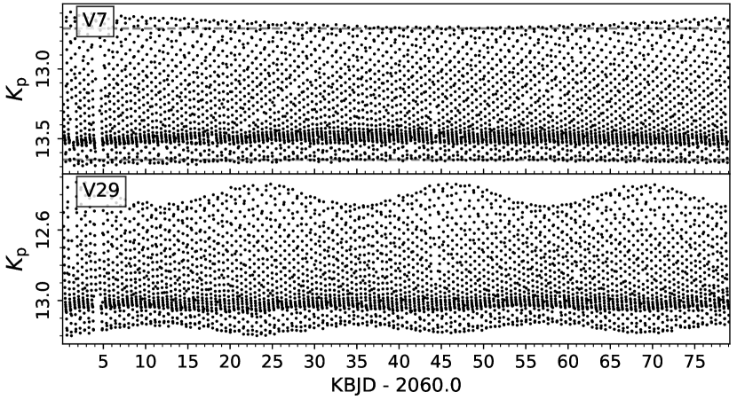
Figure 9: Light curves for V7 (candidate Blazhko variable) and V29 (Blazhko variable). The identifier is given in the upper-left corner of each panel. The x-axis scale applies to both light curves. The horizontal dashed lines in V7’s panel are arbitrary lines added to help highlight the suspected Blazhko variation.

We checked for Blazhko variations among the RR Lyrae variables by searching plots of the (unphased) light curves by eye. Stetson et al. (2014) reported V15 and V29 as candidate Blazhko variables. Kuehn et al. (2017), who used the same K2 superstamp data as us, reported V19 and V29 as Blazhko variables as detected via sidepeaks in the amplitude spectra. They also reported the V35 of Clement et al. (2001) as a Blazhko variable, but this star appeared in our edge region and so we did not extract a light curve for it. Here is what we note from our analysis, with Figure 9 showing the associated light curves for V7 and V29:

• V7: suspected Blazhko variable, with a period longer than the duration of the observation (most of a cycle is seen).

• V15: Our manual vetting did not find any Blazhko variability. As noted above, Stetson et al. (2014) marked this as a candidate Blazhko (though they did not record a period), while Kuehn et al. (2017) did not. V15 is itself a very peculiar object, as noted by Clementini et al. (1994) and we refer interested readers to that work and its references for full details. In short, the star has peculiarities in its light and radial velocity curves, which could be due either to this star being in process of transitioning from an RRAB to an RRC or a strong Blazhko variability.

• V19: Our manual vetting did not find any Blazhko variability. The sidepeak analysis of Kuehn et al. (2017) found a Blazhko period of 16.554 days.

• V29: Blazhko variable, as also noted by Kuehn et al. (2017) and listed as a candidate in Stetson et al. (2014). Kuehn et al. (2017) report a 22.419-day period, which is consistent with what we see.

V13 was first reported as a variable star in Leavitt & Pickering (1904) and is presently reported as being a semi-regular variable (SR). Eggen (1972) observed a ${\sim}$40-day variability and an amplitude of $\Delta V=0.5$ mag. In our raw light curve, we see low-amplitude variability of ${\sim}$0.1 mag, quasiperiodic with a period range of ${\sim}$20–30 days, as can be seen in Figure 8. The star is saturated in the images, so it is possible that systematics remain in our light curve. We also note that our final light curve for this object did not have any variability detected for this object, possibly due to the spline fit fitting out the long-term variability. We mention this as an example of long-term variability that can go undetected by the method employed in this work.

V66 is a ${\sim}$0.26-day contact eclipsing binary of the W Ursae Majoris type (EW by the GCVS classification). From our analysis, it was not immediately clear which of four blended stars (V66, as well as W1347, W1380, and W1426) was the source of the variability, as all four had approximately the same flux amplitude in our light curves. However, the discovery observations (Kaluzny et al., 1997) were taken at much higher resolution (median seeing FWHM ${\sim}$1$\farcs$0–1$\farcs$1 for five of the six nights of observation) than the separations of these four stars—which were comparable to but slightly greater than Kepler’s ${\sim}$4″pixel scale. We thus show the light curve only for V66 and not any of its blends.

SC3 is not a cluster member. Similar to V13, it did not have variability detected by our pipeline in its final light curve, again likely owing to the long-term and smooth nature of the variability being fitted out by our spline fit. In the raw light curve, we observe approximately the same period and amplitude of variability as Stetson et al. (2014).

SC4, not a cluster member, was identified as a variable by Stetson et al. (2014). However, Gaia DR2 has a phot_variable_flag triggered on the nearby W3152, which is a cluster member, and not SC4. Our pipeline marked SC4 as the true variable and W3152 as blended with SC4, though the flux amplitudes are within ${\sim}$15% of each other. The resolution of the images used by SC4 was sufficient to resolve these objects, which had 2$\farcs$7 separation, so we stick with Stetson et al. (2014) in calling SC4 and not W3152 the variable.

SC5 is reported as a 0.4197-day period object with ${\sim}$0.5 mag amplitude and it should have easily been detected with our data and pipeline. However, it is separated from V19—itself having a 0.4678-day period—by 7$\farcs$6 and is quite blended with it. Our pipeline did not identify any variability for SC5 at the reported period. More careful removal of V19’s signal from the data may prove fruitful for this object, but we do not perform such an analysis here.

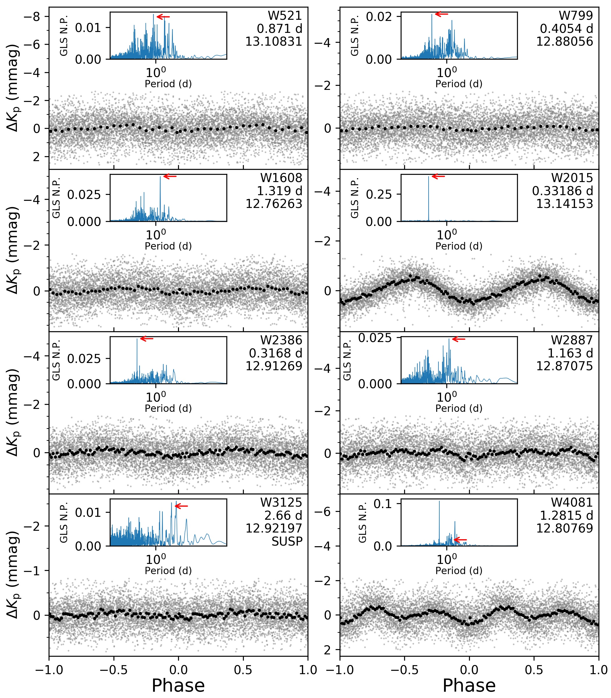
Figure 10: Phase-folded light curves and periodograms for the eight stars identified in this work as variable or suspected variable HB stars that are not RR Lyrae. Gray points show the individual magnitude measurements and the black points are binned-median values. The y-axis shows $K_{\mathrm{p}}$, in units of millimagnitude, relative to the median $K_{\mathrm{p}}$ magnitude. In the top-right corner of each panel is shown (in order from top to bottom) the object identifier, the period used for the phase folding, the median magnitude subtracted off, and, for W3125, “SUSP” indicating that this is a suspected variable. For the inset periodogram in each panel, “GLS N.P” stands for “Generalized Lomb-Scargle Normalized Power” and the red arrow points to the location in the periodogram of the phase-folding period. For W3125, the arrow points slightly off the maximum value of the peak as the period used was taken from a BLS determination of the period rather than a GLS determination. For W4081, the arrow is pointing at a period twice that of the periodogram peak, since upon visual inspection of the light curve we chose a period twice that found by GLS. In the inset x-axis and the listed period, “d” stands for “day.” W2015 and W2386 are the mmRRs from Wallace et al. (2019a).

Our pipeline also produced light curves for V54 (this work: W3012), V55 (this work: W3267), and V80 (this work: W3471), all of which are marked “CST” in the Clement et al. (2001) catalog, meaning that there is uncertainty about whether they are actually variable. Our pipeline did not flag any significant variability for any of these objects, but that does not mean they are not variable. Given the caveats of our variable-search method and the relatively low noise levels our light curves were able to reach, we decided to take a closer look at these stars, particularly their raw light curves.

V54 was marked “CST” from the time of its initial listing in the Clement et al. (2001) catalog because the first report of its variability (Yao et al. 1981a; see also Yao et al. 1981b for an English translation) reported such a small amplitude for the star and it was observed over only a ${\sim}$2-hour time window total. V54 is a giant star and a proper motion member of the cluster. It exhibits multiharmonic variability, with the strongest GLS power at ${\sim}$1.02-day period, with a ${\sim}$1 mmag variability. The reason this was not detected by our method is likely the rich structure of the periodogram boosted the noise value used in the periodogram SNR calculation, thus leading to an SNR value that fell below the threshold. This variability, though, is of ${\sim}$1 mmag amplitude, much smaller than the ${\sim}$0.1–0.2 mag seen for this star in Yao et al. (1981a) and is probably unrelated to what they reported.

V55 was also first reported by Yao et al. (1981a, b) and was also marked “CST” from its initial entry into the Clement et al. (2001) catalog for the same reasons as V54. V55 is an HB star and a proper motion member of the cluster. The variability amplitude reported by Yao et al. (1981a) for V55 (${\sim}$0.1–0.2 mag) is larger than the ${\sim}$3 mmag RMS value we obtain for the raw light curve or the ${\sim}$0.3 mmag RMS noise value we obtain for the final light curve. The strongest GLS period is ${\sim}$3.10 day, but this is somewhat weak and the periodogram overall is fairly noisy.

V80 is a subgiant member of the cluster. Variability was reported by Yao et al. (2007) (see Yao et al. 2006b for an English translation) as variable with a period of about a day and with amplitude of 0.05 mag in $V$. Despite our obtaining an RMS noise level of ${\sim}$0.01 mag in its raw light curve and ${\sim}$3 mmag in its final light curve, no significant variability is seen.

Thus from our work we think V54 should be marked a low-amplitude asteroseismic variable and V55 and V80 retain their “CST” designations, though it would seem the variability we observe for V54 is not the same variability, or at least significantly changed from, what was reported by Yao et al. (1981a).

3.3 Millimagnitude RR Lyrae and the Other Horizontal Branch Stars

Two of the HB stars—W2015 and W2386—have been more fully examined in Wallace et al. (2019a) as potential low-amplitude RRC pulsators (millimagnitude RR Lyrae variables, or mmRRs as coined in that work). W2015 is mmRR 1 from that work, W2386 is mmRR2, and W4081 is G3168 briefly mentioned in that work. We define the HB in similar fashion as Wallace et al. (2019a): stars with $14.3\,<\,G_{\mathrm{BP}}\,<\,13.0$ and $G_{\mathrm{BP}}-G_{\mathrm{RP}}\,<\,1.5$ and a ${>}$95% cluster membership probability (though the membership probabilities for all these stars are so high that a 99% cutoff could be used with no loss). Excluding the 10 stars previously identified as RR Lyrae variables (see Table 2), we have light curves for 24 HB stars, eight of which we detected as significantly variable. Information on these HB variables is found in Table 3, and Figure 10 shows the phase-folded light curves and GLS periodograms for these objects. We stress once again, though, that our periodogram SNR cutoff can sometimes exclude stars with significant variability at other periods close to the peak period, so it is entirely possible that multiharmonic variability is to be found among many of the other 16 non-RR-Lyrae HB stars. Indeed, a quick search that we performed revealed many of them—though not all—to possess multiharmonic variability. To maintain internal consistency with our search method, we do not report them in detail here, but do note again our light curves are available for download and analysis at Wallace et al. (2019b). Several of these objects are blended with other bright stars, so we advise appropriate caution in using them. Two particularly notable blends we noticed were W818, which is likely a blend with W1189; and W1607, which is either blended or otherwise left with a photometric footprint of the somewhat distant V10. W1607 has some power in its periodogram outside the blend period and may possess intrinsic variability. Likewise, W1628 and W1643 are blended with V61 and V9 and may require a more careful analysis.

Interpreting the previously identified mmRRs in the context of these additional HB variables is informative. Given that the periodogram structures seem to form a continuum between the strongly mono-periodic W2015 and the rich, very multi-periodic periodogram of W521, it is possible that what we have called mmRRs are a transition between the asteroseismic variability of HB stars outside of the instability strip and the RR Lyrae pulsators inside. We note that W2015/mmRR 1 and W3125 are blueward of the instability strip, W4081 is inside the strip, and the remaining objects are redward. There still remain many questions. Why does W2015 (mmRR1) have such a single dominant period whereas the other HBs do not have any periods with such great prominence? What causes the range of periods seen? What causes W4081’s striking even-odd amplitude modulation, and why is it found in the instability strip but not pulsating like the RR Lyrae variables? Certainly the K2 photometric precision and the observations of concentrations of HB stars in GCs allows for an unprecedented look at the asteroseismic variations of HB stars outside the instability strip in addition to the RR Lyrae variables themselves. We also echo our previous caveat that other HB stars with rich periodogram structures may have been missed by our period search method, and these may not be the only HB stars with detectable oscillations.

3.4 Other Cluster Variables

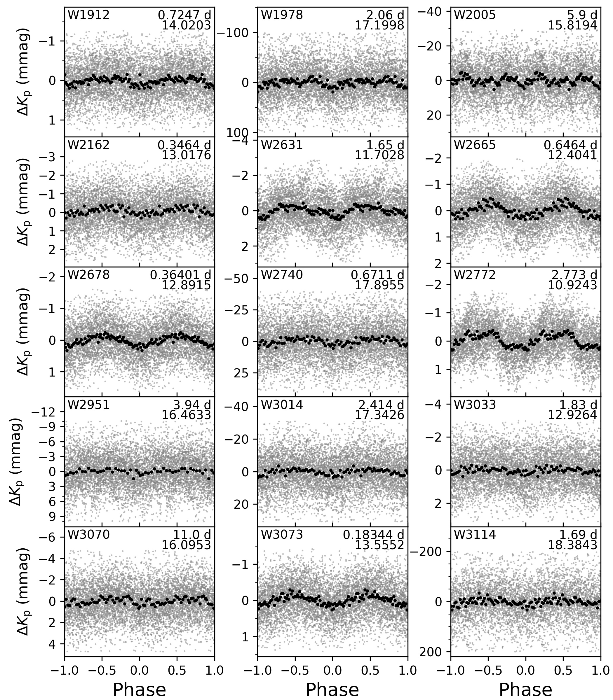
Figure 12: Same as Figure 11, but for additional cluster member variables.

Table 3 shows information for the variable cluster members, both proper and suspected variables. The suspected variables are more thoroughly discussed and presented in Appendix B. Figures 11, 12, and 13 show the phase-folded light curves for the variables. We discuss here and in Section 3.5 some of the more notable cluster-member variables.

W4490 has a particularly interesting light curve: a 1.959-day period triangular-shaped increase in brightness, with an amplitude of ${\sim}$20 mmag. Figure 13 plots the phase-folded raw light curve instead of the processed, final light curve. We found that the processing cut its amplitude approximately in half. The raw light curve has systematic noise, most likely due to this object’s period being very close to the resaturation period (1.962 days) and nearly an integer multiple of the drift correction and observing cadence. Verbunt (2001) reports a ROSAT X-ray source detection 2$\farcs$8 away from this object (object X8 in NGC6121/M4), with a reported position statistical error on the X-ray source of 2$\farcs$6 and an additional projection error of ${\sim}$5″also at play. This spatially coincident X-ray source with the reported variability period have informed our classification of this object as an X-ray binary. This portion of M4 unfortunately has not been included in fields of view of previous Chandra observations, which have been primarily focused on the cluster’s core (e.g. Bassa et al., 2004). Its unusual photometry was noted in Section 3.1 and Figure 6. As measured by Gaia DR2, this object is much more red than we would expect for a star of its luminosity in the cluster.

Of the other cluster-member variables in Figures 11–13, most are low-amplitude sinusoids, possibly including some ellipsoidal or rotational variables. Many are giant stars showing mmRR or multiharmonic asteroseismic variability. For those objects the periods shown in the figures are typically just the dominant sinusoidal component. In Figure 7, it can be seen in the top-left panel that these stars appear to extrapolate the period–luminosity relationship of the RR Lyrae, with variables of longer period than the RR Lyrae variables continuing the relation of the RRABs (the cluster of diamonds with period greater than 0.4 days), the handful of objects with periods less than the RRCs (the two diamonds with periods ${\sim}$0.3 days) seeming to form a parallel trend, and objects falling into the period range of the RR Lyrae variables themselves having similar $G$ magnitudes as them. Since $G$ is correlated with evolutionary state for these stars, and thus with stellar density, it is not surprising that the oscillation periods, which are determined in part by stellar densities, are correlated with $G$ even for smaller-amplitude oscillators than the RR Lyrae variables. The scatter seen in the relation is probably due to the picking up different modes for different stars as the dominant cause of the photometric variability. We also note an apparent correlation between amplitude and period in the lower-right panel of Figure 7 for the multiharmonic and mmRR stars.

There were a number of variable signals that were indistinguishably blended between two or more stars and that were not able to be disentangled either from our data or from referencing some other previous work of which we knew. Table 4 lists these objects, both cluster members and nonmembers, and Figure 14 shows the associated light curves. W283/W293, and W1318/W1335/W1246, both EWs, are discussed in Section 3.5.

Table 3: Newly Discovered Cluster Variables

ID	R.A.	decl.	$G$	Period	Per. Unc.	Amp.	Epoch	Method	Type
	(hh:mm:ss)	(dd:mm:ss)	(mag)	(day)	(10-4 day)	(mmag)	(KBJD)
Variables
W491	16:23:11.52	$-$26:26:41.1	13.37	0.27941	0.6	0.3	2060.51	Harm.	mmRR/mh
W508	16:23:12.04	$-$26:29:44.0	13.86	0.16280	0.3	0.2	2060.40	Harm.	mh
W521	16:23:12.36	$-$26:21:58.8	13.25	0.871	10	0.4	2060.45	Harm.	mh
W566	16:23:13.39	$-$26:29:15.7	17.82	0.28870	0.9	2	2060.50	Harm.	EW?
W689	16:23:15.73	$-$26:25:58.0	15.47	0.992	10	0.7	2061.21	Harm.	EA?
W799	16:23:17.63	$-$26:27:10.6	13.01	0.4054	7	0.2	2060.41	Harm.	mh
W837	16:23:18.22	$-$26:29:07.6	14.39	0.09472	0.1	0.1	2060.37	Harm.	shortperiod
W869	16:23:18.68	$-$26:23:43.6	10.76	2.177	20	0.3	2061.98	Harm.	mh
W1091	16:23:21.68	$-$26:26:47.2	13.05	0.3583	1	0.3	2060.44	Harm.	mh
W1154	16:23:22.5	$-$26:24:59.4	16.15	0.991	20	0.6	2060.66	Harm.	?
W1165	16:23:22.64	$-$26:26:22.5	12.08	1.3338	5	0.8	2061.10	Harm.	mh
W1349	16:23:24.98	$-$26:29:25.3	13.23	0.3884	2	0.2	2060.43	Harm.	mh
W1582	16:23:27.84	$-$26:29:11.9	13.78	0.17275	0.4	0.2	2060.36	Harm.	mh
W1601	16:23:28.07	$-$26:25:02.2	19.11	4.6337	9	38	2063.48	Trap.	EA
W1608	16:23:28.13	$-$26:26:08.9	12.90	1.319	10	0.2	2061.60	Harm.	mh
W1735	16:23:29.5	$-$26:29:12.0	11.65	2.146	20	1	2062.10	Harm.	mh
W1763	16:23:29.81	$-$26:23:25.6	12.51	0.7836	8	0.4	2060.63	Harm.	mh
W1848	16:23:30.51	$-$26:23:57.9	17.59	0.4486	4	3	2060.33	Harm.	?
W1912	16:23:31.28	$-$26:25:16.1	14.18	0.7247	8	0.2	2060.98	Harm.	?
W1978	16:23:31.99	$-$26:29:38.1	18.61	2.06	100	18	2062.19	Harm.	?
W2005	16:23:32.21	$-$26:27:01.4	16.35	5.9	5000	5	2060.66	Harm.	?
W2015	16:23:32.3	$-$26:28:53.5	13.23	0.33186	0.3	0.9	2060.39	Harm.	mmRR
W2162	16:23:33.79	$-$26:27:50.0	13.15	0.3464	2	0.4	2060.62	Harm.	mh
W2386	16:23:35.93	$-$26:26:20.9	13.05	0.3168	1	0.2	2060.59	Harm.	mmRR/mh
W2631	16:23:38.46	$-$26:29:23.9	11.84	1.65	200	0.7	2061.29	Harm.	mh
W2665	16:23:38.84	$-$26:25:43.1	12.56	0.6464	2	0.5	2060.55	Harm.	mh
W2678	16:23:38.93	$-$26:22:09.8	13.05	0.36401	0.8	0.3	2060.32	Harm.	mmRR?/mh
W2740	16:23:39.68	$-$26:24:36.7	18.20	0.6711	9	4	2060.60	Harm.	?
W2772	16:23:39.97	$-$26:28:49.3	11.06	2.773	30	0.6	2062.79	Harm.	mh
W2887	16:23:41.33	$-$26:29:09.1	13.00	1.163	30	0.4	2060.44	Harm.	mh
W2951	16:23:42.14	$-$26:28:47.7	16.67	3.94	200	0.8	2063.90	Harm.	?
W3014	16:23:42.83	$-$26:25:31.6	17.41	2.414	80	3	2060.64	Harm.	?
W3033	16:23:43.08	$-$26:28:07.8	13.06	1.83	300	0.3	2061.75	Harm.	mh
W3070	16:23:43.47	$-$26:23:28.7	16.24	11.0	7000	0.7	2066.27	Harm.	?
W3073	16:23:43.51	$-$26:25:37.8	13.70	0.18344	0.2	0.3	2060.32	Harm.	mh
W3114	16:23:44.02	$-$26:29:31.8	18.81	1.69	100	22	2061.77	Harm.	?
W3259	16:23:45.81	$-$26:28:35.4	18.91	1.734	60	5	2060.84	Harm.	?
W3407	16:23:47.97	$-$26:28:21.9	18.54	2.352	30	8	2061.13	Harm.	?
W3430	16:23:48.3	$-$26:22:42.6	17.50	0.5107	3	3	2060.37	Harm.	?
W3480	16:23:48.98	$-$26:29:19.6	13.31	0.25657	0.7	0.3	2060.29	Harm.	mmRR?/mh
W3485	16:23:49.08	$-$26:28:27.4	14.71	1.411	30	0.3	2061.51	Harm.	?
W3742	16:23:52.99	$-$26:28:06.9	13.03	0.32514	0.8	0.3	2060.37	Harm.	mmRR/mh
W3957	16:23:57.1	$-$26:25:36.5	18.61	0.995	20	15	2061.20	Harm.	?
W3996	16:23:57.71	$-$26:22:56.1	11.73	3.054	50	0.8	2061.88	Harm.	mh
W4081	16:23:59.3	$-$26:27:15.8	12.93	1.2815	9	0.9	2061.10	Harm.	mmRR/mh
W4237	16:24:04.17	$-$26:27:03.1	15.87	0.09282	0.2	0.3	2060.35	Harm.	shortperiod
W4333	16:24:07.73	$-$26:28:41.4	16.65	0.3618	3	0.6	2060.30	Harm.	EA?
W4361	16:24:08.57	$-$26:24:55.5	11.36	4.768	30	0.7	2065.02	Trap.	EB
W4490	16:24:14.75	$-$26:27:51.2	15.62	1.959	10	11	2060.99	Harm.	xrb
Suspected Variables
W58	16:22:57.25	$-$26:28:44.3	18.78	0.2228	3	39	2060.44	Harm.	…
W267	16:23:05.52	$-$26:27:01.1	17.82	2.76	100	2	2060.99	Harm.	…
W371	16:23:09.14	$-$26:30:00.4	15.70	0.2461	2	0.3	2060.48	Harm.	…
W435	16:23:10.35	$-$26:29:31.1	16.58	0.2468	2	0.3	2060.37	Harm.	…
W461	16:23:10.94	$-$26:26:33.3	17.64	3.90	300	13	2061.24	Harm.	…
W829	16:23:18.1	$-$26:21:44.1	18.17	7.9	8000	5	2064.10	Harm.	…
W901	16:23:19.17	$-$26:27:52.4	17.12	0.2121	2	0.7	2060.40	Harm.	…
W920	16:23:19.49	$-$26:25:47.2	17.17	0.3321	2	0.7	2060.52	Harm.	…
W1056	16:23:21.29	$-$26:28:44.9	17.95	25.66	500	21	2079.96	Trap.	…
W1068	16:23:21.4	$-$26:28:33.9	13.85	1.256	20	0.2	2060.88	Harm.	…
W1208	16:23:23.17	$-$26:26:02.9	18.23	0.315311	0.06	3	2060.37	Harm.	…
W1222	16:23:23.35	$-$26:29:24.2	18.60	11.679	80	15	2064.54	Trap.	…
W1263	16:23:23.87	$-$26:26:04.9	16.33	5.830	50	1	2064.15	Trap.	…
W1539	16:23:27.42	$-$26:26:25.5	17.60	0.13900	0.9	2	2060.31	Harm.	…
W1717	16:23:29.37	$-$26:26:28.0	13.98	0.12580	0.3	0.1	2060.40	Harm.	…
W1725	16:23:29.43	$-$26:28:17.7	16.67	0.18434	0.8	0.9	2060.44	Harm.	…
W1809	16:23:30.13	$-$26:21:36.7	18.56	14.14	200	4	2071.16	Trap.	…
W1834	16:23:30.39	$-$26:28:23.2	17.53	9.29	300	$-$2	2065.57	Trap.	…
W1864	16:23:30.74	$-$26:27:27.7	17.48	4.3	2000	15	2060.93	Harm.	…
W1938	16:23:31.53	$-$26:27:49.8	17.48	3.4391	10	4	2061.64	Trap.	…
W1947	16:23:31.63	$-$26:29:23.6	18.99	1.597	60	12	2061.19	Harm.	…
W1953	16:23:31.68	$-$26:28:06.8	18.00	2.34	400	1	2061.42	Harm.	…
W2109	16:23:33.19	$-$26:28:10.7	17.19	0.5065	2	4	2060.69	Harm.	…
W2126	16:23:33.42	$-$26:29:39.2	17.55	2.66	200	5	2062.22	Harm.	…
W2127	16:23:33.45	$-$26:29:29.7	17.98	…	…	${\sim}-40$	${\sim}2096$	…	…
W2233	16:23:34.48	$-$26:26:29.6	18.91	0.46817	0.3	5	2060.29	Harm.	…
W2272	16:23:34.85	$-$26:26:04.6	18.74	2.223	70	26	2062.05	Harm.	…
W2324	16:23:35.27	$-$26:23:31.2	17.76	1.53	200	2	2060.89	Harm.	…
W2499	16:23:37.11	$-$26:28:45.6	16.72	3.832	40	10	2062.90	Harm.	…
W2515	16:23:37.28	$-$26:28:08.5	19.11	1.408	10	8	2061.36	Harm.	…
W2543	16:23:37.6	$-$26:27:20.3	16.10	31.07	500	1	2073.32	Trap.	…
W2556	16:23:37.7	$-$26:27:20.4	16.03	33.96	900	1	2079.36	Trap.	…
W2577	16:23:37.94	$-$26:28:41.7	13.01	3.20	100	0.4	2062.23	Harm.	…
W2616	16:23:38.3	$-$26:29:03.4	18.45	3.81	200	40	2060.81	Harm.	…
W2641	16:23:38.58	$-$26:29:11.7	14.43	0.8678	7	2	2061.11	Harm.	…
W2747	16:23:39.74	$-$26:29:32.8	17.19	7.091	80	4	2067.02	Harm.	…
W2753	16:23:39.78	$-$26:29:42.1	18.44	0.5474	5	9	2060.42	Harm.	…
W2790	16:23:40.27	$-$26:27:37.8	17.42	6.36	200	$-$2	2064.21	Trap.	…
W2800	16:23:40.4	$-$26:28:20.6	17.87	1.84	200	5	2061.85	Harm.	…
W2819	16:23:40.61	$-$26:29:02.1	18.31	1.66	200	120	2060.77	Harm.	…
W2876	16:23:41.22	$-$26:28:53.0	16.64	4.203	90	5	2062.41	Harm.	…
W2893	16:23:41.41	$-$26:23:18.0	17.83	1.28	200	1	2060.63	Harm.	…
W2966	16:23:42.25	$-$26:27:42.2	15.75	0.372	20	0.2	2060.63	Harm.	…
W3105	16:23:43.88	$-$26:27:36.8	16.83	0.6060	3	4	2060.33	Harm.	…
W3125	16:23:44.21	$-$26:28:24.4	13.00	2.66	500	0.1	2061.01	Harm.	…
W3282	16:23:46.11	$-$26:25:34.7	17.37	2.50	200	1	2061.92	Harm.	…
W3313	16:23:46.53	$-$26:28:41.7	17.66	3.978	40	6	2063.97	Trap.	…
W3371	16:23:47.31	$-$26:22:30.4	13.91	0.966	20	0.2	2060.42	Harm.	…
W3521	16:23:49.59	$-$26:29:30.8	18.84	2.692	100	22	2060.45	Harm.	…
W3552	16:23:50.08	$-$26:29:33.4	14.78	9.0	7000	1	2063.41	Harm.	…
W3887	16:23:55.53	$-$26:28:34.0	17.26	2.443	30	1	2062.30	Trap.	…
W3901	16:23:55.82	$-$26:29:20.8	17.11	0.522	30	0.9	2060.79	Harm.	…
W4014	16:23:58.03	$-$26:23:30.4	18.47	1.88	400	12	2060.28	Harm.	…
W4143	16:24:01.17	$-$26:25:13.6	17.27	3.403	20	2	2063.22	Trap.	…
W4250	16:24:04.81	$-$26:24:17.4	19.01	1.784	20	33	2060.90	Harm.	…
W4268	16:24:05.39	$-$26:29:16.2	17.31	1.983	10	2	2061.75	Harm.	…
W4301	16:24:06.43	$-$26:28:53.3	18.70	4.283	20	5	2062.69	Trap.	…

Note. — Classifications are not attempted for the suspected variables. Explanations regarding why these are reported as suspected instead of discovered variables can be found in Appendix B.

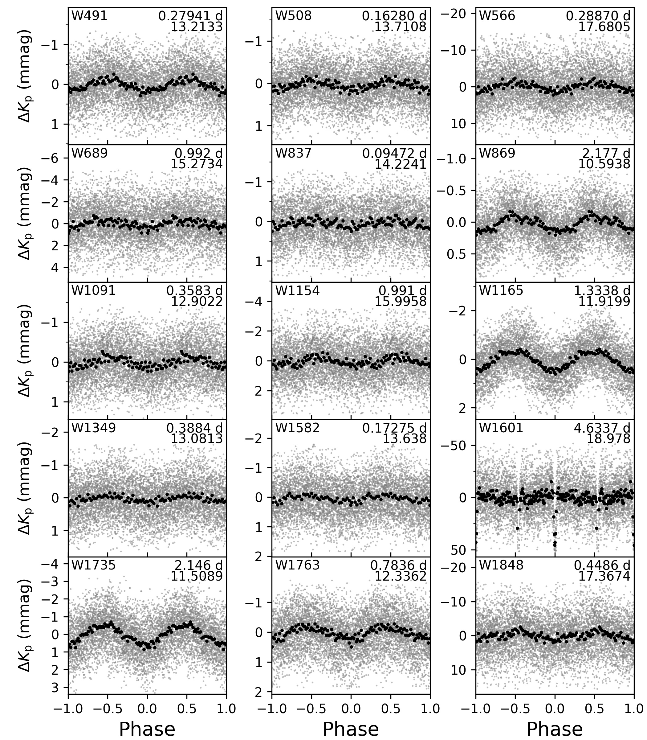
Figure 11: Phase-folded light curves for cluster members that, other than W2665 and W3033, are newly identified as variable stars in this work. W2665 and W3033 were previously identified by Miglio et al. (2016). The panels are ordered by the target identifier. Here we show the first 15 cluster variables. Additional variables are shown in Figures 12 and 13. Gray points show the individual magnitude measurements and the black points are binned-median values. The y-axis shows $K_{\mathrm{p}}$, in units of millimagnitude, relative to the median $K_{\mathrm{p}}$ magnitude. In each panel, the identifier of the star is shown in the upper left corner, and (from top to bottom) the folding period and subtracted median magnitude are shown in the upper right corner. For the listed period, “d” stands for “day.”

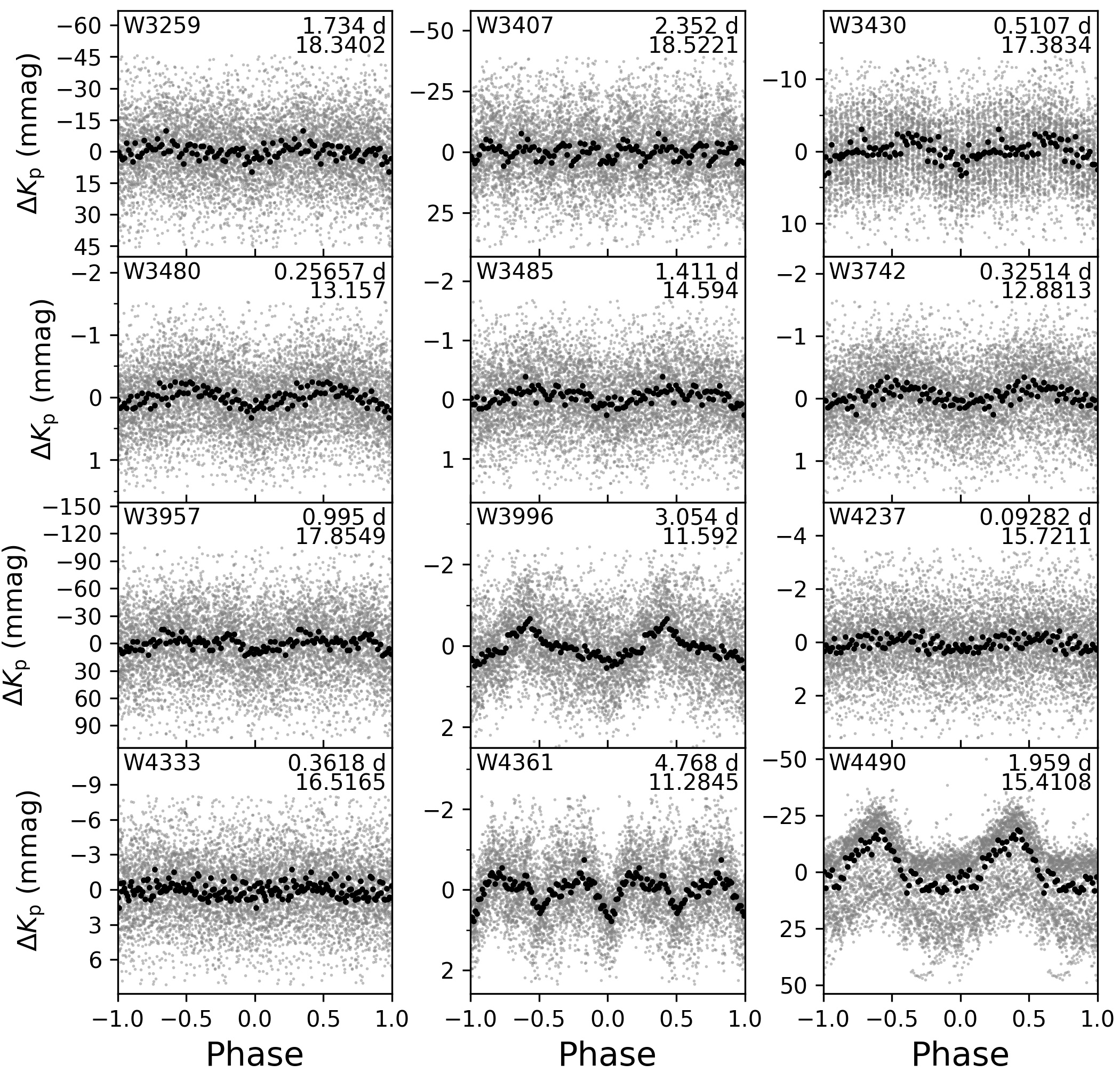
Figure 13: Same as Figures 11 and 12, but for additional cluster member variables. The data from W4490 are taken from its raw light curve.

Table 4: Newly Discovered Variables that are Indeterminable Blends

ID	R.A.	decl.	$G$	Period	Per. Unc.	Amp.	Epoch	Type	Mem. Prob.
	(hh:mm:ss)	(dd:mm:ss)	(mag)	(day)	(10-4 day)	(mmag)	(KBJD)
Blended Stars All Cluster Members
W283	16:23:06.14	$-$26:27:45.8	18.28	0.20450	0.3	6	2060.40	EW	1.00
W293	16:23:06.46	$-$26:27:50.9	19.08	0.20450	0.1	23	2060.40	EW	1.00
W1129	16:23:22.23	$-$26:28:00.3	17.71	0.967	20	3	2060.60	?	1.00
W1136	16:23:22.29	$-$26:28:03.7	15.80	0.967	10	0.8	2060.55	?	1.00
W1146	16:23:22.38	$-$26:27:59.3	17.77	0.969	20	3	2060.46	?	1.00
W2262	16:23:34.78	$-$26:29:15.1	17.38	0.5003	10	4	2060.63	?	1.00
W2282	16:23:34.95	$-$26:29:14.2	18.32	0.50016	0.5	8	2060.61	?	1.00
W2289	16:23:34.99	$-$26:29:10.4	18.86	…	…	…	…	…	1.00
W2300	16:23:35.08	$-$26:29:12.7	16.97	0.4989	1	2	2060.65	?	1.00
W2826	16:23:40.66	$-$26:29:27.8	16.87	2.004	40	2	2060.53	?	1.00
W2830	16:23:40.69	$-$26:29:30.4	17.63	2.00	100	4	2060.54	?	1.00
W3431	16:23:48.31	$-$26:28:13.4	17.41	0.5887	4	3	2060.47	EW?	1.00
W3436	16:23:48.42	$-$26:28:13.7	17.51	0.5889	4	3	2060.47	EW?	1.00
W3456	16:23:48.64	$-$26:28:14.8	17.87	0.5887	4	4	2060.46	EW?	1.00
Blended Stars Mixed Between Cluster Members and Non- or Ambiguous Members
W1318	16:23:24.57	$-$26:26:23.0	18.97	0.277389	0.07	270	2060.34	EW	1.00
W1335	16:23:24.86	$-$26:26:22.8	18.37	0.27742	0.9	180	2060.33	EW	…
W1346	16:23:24.95	$-$26:26:28.8	18.00	0.277415	0.09	51	2060.33	EW	1.00
W2006	16:23:32.23	$-$26:22:48.3	18.69	2.440	40	16	2062.01	?	1.00
W2013	16:23:32.29	$-$26:22:44.2	18.55	2.440	20	18	2062.03	?	0.00
W2761	16:23:39.86	$-$26:29:24.5	16.81	1.0002	10	4	2060.68	EW?	1.00
W2779	16:23:40.17	$-$26:29:26.1	18.11	1.000	20	8	2060.54	EW?	1.00
W2793	16:23:40.28	$-$26:29:26.2	17.14	1.000	20	4	2060.68	EW?	1.00
W2813	16:23:40.55	$-$26:29:23.5	18.86	0.998	40	8	2060.76	EW?	0.00
W3883	16:23:55.35	$-$26:24:51.0	17.43	2.583	60	2	2062.05	EA?	1.00
W3894	16:23:55.62	$-$26:24:52.6	16.83	2.590	60	1	2062.10	EA?	0.73

Note. — All amplitudes and epochs calculated using a harmonic fit, compared to Tables 3 and 5 where some were determined with a trapezoid fit

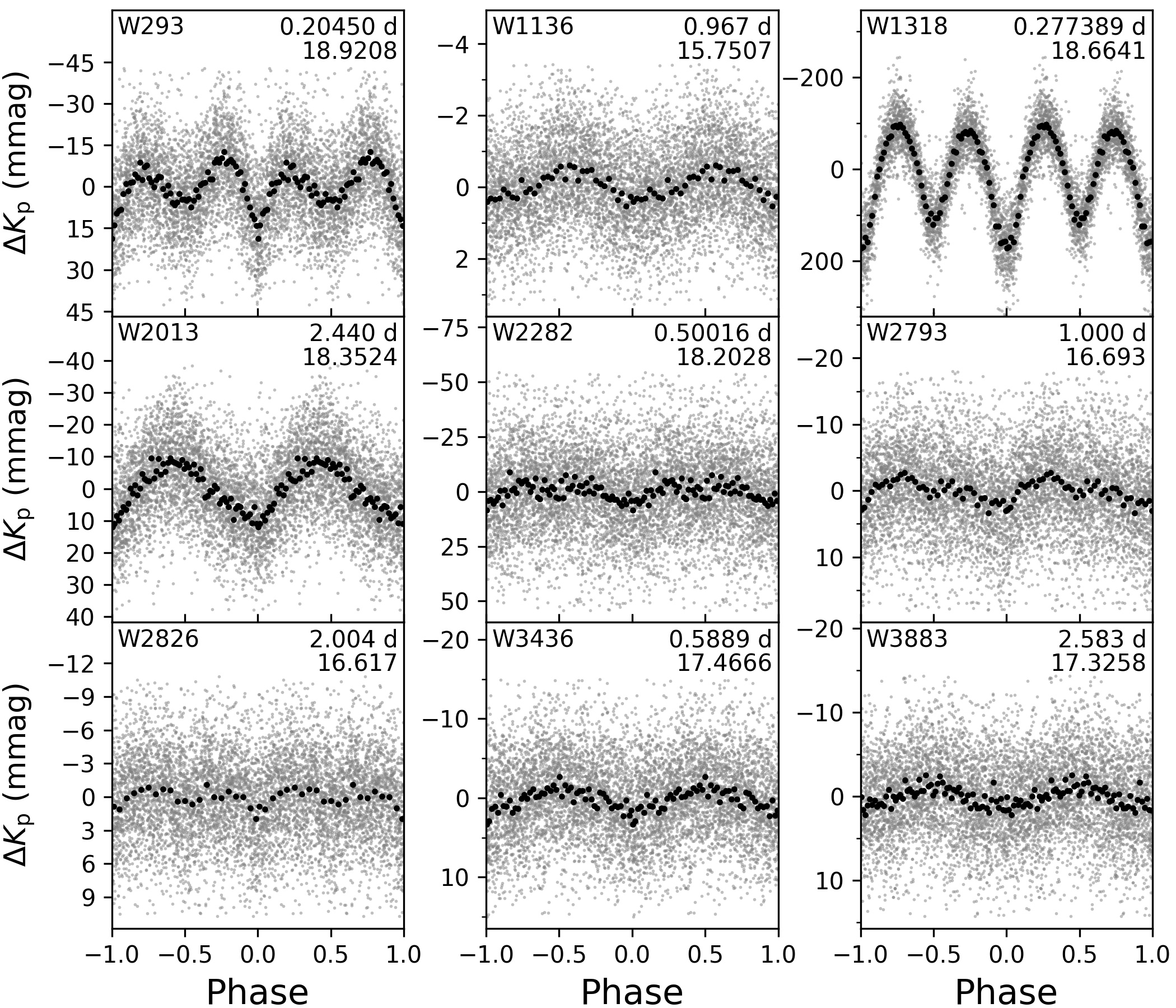
Figure 14: Same as Figure 11, but for stars with signals that are indistinguishably blended in our data. In each case, only one star from each set of blended stars is chosen to represent the light curve. See Table 4 for more information.

3.5 Cluster Eclipsing and Contact Binaries

W1601, shown in Figure 11, is a detached eclipsing binary with a 4.6337-day period. The phase difference between the primary and secondary eclipses reveals the system to be slightly eccentric. The system appears to be grazing, with a primary eclipse depth of $0.038\pm 0.005$ mag, a fractional duration of $0.046\pm 0.003$, and an eclipse ingress fractional duration of $0.016\pm 0.004$, making the eclipse very triangular. There is also a sinusoidal variability on top of the eclipses, suggesting ellipsoidal variability, not terribly surprising considering the short period of the binary. This informs our classification of this as an Algol-type eclipsing binary (EA). Based on the Clement et al. catalog, this is the sixth EA known in M4, with the note that the two EAs of Safonova et al. (2016) are not cluster members based on the proper motions reported there.

W4361, shown in Figure 13, is possibly another eclipsing binary. In this case the system appears to be semi-detached or maybe even contact binary. The eclipses are very triangular. The depth of the primary eclipse based on our trapezoid fit is $0.72\pm 0.05$ mmag, with a fractional eclipse duration of $0.21\pm 0.01$ and fractional ingress duration of $0.07\pm 0.01$. This is a red giant star, with a radius that should be much larger than the ${\sim}$15 R_☉ implied by the orbital period and the ${\sim}$0.8 M_☉ maximum expected masses for each of the stars given their membership in the cluster. Perhaps W4361 is simply blended with a background eclipsing binary or even another binary in the cluster.

W293, blended with W283, is a clear example of an EW, having a period of 0.20450 days and a primary eclipse depth of ${\sim}$30 mmag and a secondary eclipse depth of approximately half that. Both stars are cluster members. Similarly, W1318, blended with W1335 and W1346, is also a clear EW. The orbital period is 0.277389 days and the primary eclipse depth is ${\sim}$20 mmag and the secondary eclipse depth ${\sim}$10 mmag. W1318 and W1346 are proper motion members of the cluster, but W1335 does not have reported proper motions in Gaia DR2. However, based on its CMD location ($G{\approx}18.4$, $G_{\mathrm{BP}}-G_{\mathrm{RP}}{\approx}1.44$), it is a probable cluster member, and so we report a high degree of certainty that this EW also belongs to the cluster. There are also two other suspected EWs: W3431/W3436/W3456, all three of which are cluster members, and W2761/W2779/W2793/W2813, of which all but the last are cluster members.

3.6 Variables Not In M4

Included with the rich variety of cluster-member variables are many variables that were not cluster members. Table 5 shows information for these variable stars, and Figures 15 and 16 show the phase-folded light curves. The suspected variables will be more thoroughly discussed in Appendix B.

At ${\sim}$1.8 kpc in distance, and also being relatively close to the Galactic center ($l{\approx}351\arcdeg,b{\approx}16\arcdeg$), the non-cluster-member stars in the direction of M4 are a mixture of both foreground and background objects. We will touch on only two of the field variables here.

W1189 is also HD 147491 and V972 Sco of the GCVS. Yao & Tong (1989) reported this star as being a DSCUT variable with a ${\sim}$0.02-day period; however, we do not see any ${\sim}$0.02-day variability, and the 1.5097 day period we find is too long for a DSCUT. We think it is more likely that this is a gamma Doradus variable (GDOR). This is also the brightest star in the M4 superstamp, with Gaia DR2 $G=9.46$.

W3756 is also V1331 Sco of the GCVS. Yao et al. (2006a) identified a ${\sim}$15 mmag, 1.03-day period variability in this star based on $V$-band observations taken in 1990 and 1991 and classified it as a GDOR. We see a ${\sim}$1 mmag amplitude and a 0.634-day period. There is also power in our GLS, PDM, and BLS periodograms for this object at a period ${\sim}$0.97 days (compare with the original 1.03-day period in the discovery), which is the dominant periodogram peak when the main period and its harmonics are removed. GDOR variability can change in amplitude and dominant frequency over time. This combined with the differences between the $K_{\mathrm{p}}$ and $V$ bandpasses make it unsurprising for us to see a different amplitude and dominant period relative to the Yao et al. (2006a) observations, made over 23 years prior the K2 observations.

W2203 is a detached eclipsing binary with a 21.72-day period and what appears to be reflections or other brightening events just before and after both the primary and secondary eclipses. The primary eclipse depth is $0.013\pm 0.001$ mag, with a fractional eclipse duration of $0.028\pm 0.003$ and a fractional ingress duration of $0.005\pm 0.002$.

Finally, we remind the reader of the blended variables in Table 4 and Figure 14 that are not cluster members: W2013 (blended with W2006) and W2813 (blended with W2761, W2779, and W2793).

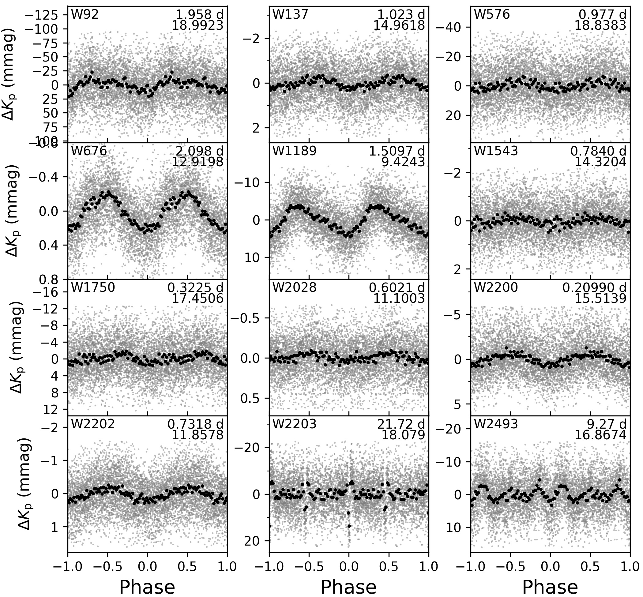
Figure 15: Same as Figure 11, but for variables that are not cluster members. 12 variables are shown in this figure, and Figure 16 shows the remaining 10.

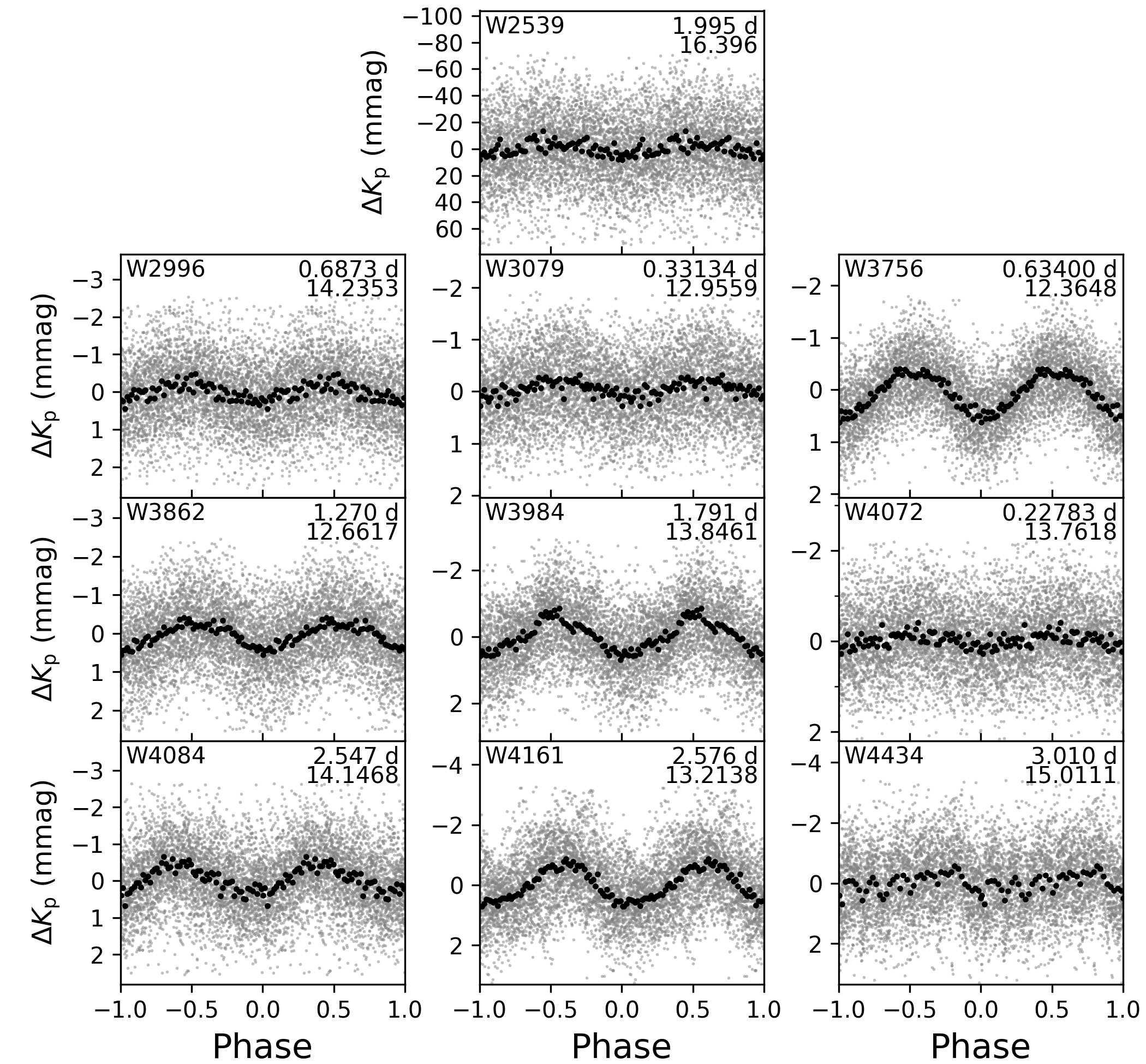
Figure 16: Same as Figure 15, but for additional variables that are not cluster members.

Table 5: Newly Discovered Variables that are Not Cluster Members

ID	R.A.	decl.	$G$	Period	Per. Unc.	Amp.	Epoch	Method	Type
	(hh:mm:ss)	(dd:mm:ss)	(mag)	(day)	(10-4 day)	(mmag)	(KBJD)
Variables
W92	16:22:58.62	$-$26:28:59.7	19.09	1.958	60	24	2061.98	Harm.	?
W137	16:23:00.83	$-$26:25:22.2	15.10	1.023	20	0.4	2061.26	Harm.	?
W576	16:23:13.64	$-$26:26:27.8	18.89	0.977	10	5	2061.13	Harm.	?
W676	16:23:15.54	$-$26:27:46.3	13.03	2.098	10	0.4	2061.24	Harm.	?
W1189	16:23:22.91	$-$26:22:16.0	9.46	1.5097	5	8	2060.99	Harm.	GDOR?
W1543	16:23:27.47	$-$26:23:11.9	14.44	0.7840	7	0.3	2060.94	Harm.	?
W1750	16:23:29.66	$-$26:21:13.9	17.63	0.3225	2	2	2060.55	Harm.	?
W2028	16:23:32.46	$-$26:26:45.0	11.18	0.6021	5	0.07	2060.37	Harm.	?
W2200	16:23:34.14	$-$26:25:50.2	15.65	0.20990	0.5	1	2060.29	Harm.	?
W2202	16:23:34.15	$-$26:23:53.9	12.02	0.7318	3	0.4	2060.44	Harm.	?
W2203	16:23:34.17	$-$26:21:39.3	18.23	21.72	100	13	2064.83	Trap.	E/EA?
W2493	16:23:37.04	$-$26:21:51.7	16.98	9.27	300	5	2069.21	Harm.	?
W2539	16:23:37.58	$-$26:29:18.4	17.20	1.995	40	8	2061.83	Harm.	?
W2996	16:23:42.58	$-$26:23:43.9	14.42	0.6873	4	0.5	2060.76	Harm.	?
W3079	16:23:43.58	$-$26:26:18.4	13.12	0.33134	1	0.2	2060.55	Harm.	?
W3756	16:23:53.21	$-$26:22:24.5	12.47	0.63400	1	0.8	2060.47	Harm.	GDOR
W3862	16:23:54.98	$-$26:26:10.8	12.83	1.270	30	0.7	2061.27	Harm.	?
W3984	16:23:57.56	$-$26:23:24.5	14.02	1.791	10	1	2061.13	Harm.	?
W4072	16:23:59.18	$-$26:23:30.8	13.92	0.22783	0.5	0.3	2060.47	Harm.	mh
W4084	16:23:59.36	$-$26:29:10.5	14.26	2.547	30	0.8	2062.71	Harm.	?
W4161	16:24:01.82	$-$26:27:32.4	13.37	2.576	40	1	2061.39	Harm.	mh
W4434	16:24:11.6	$-$26:28:26.1	15.15	3.010	80	0.7	2063.07	Harm.	?
Suspected Variables
W55	16:22:57.19	$-$26:29:09.1	18.22	1.85	100	7	2061.59	Harm.	…
W126	16:23:00.36	$-$26:27:32.7	18.92	0.041004	0.03	8	2060.29	Harm.	…
W951	16:23:19.93	$-$26:27:54.2	17.13	5.8	1000	1	2064.83	Harm.	…
W1779	16:23:29.93	$-$26:26:53.5	15.88	4.76	700	4	2063.40	Harm.	…
W2571	16:23:37.87	$-$26:21:57.6	18.77	2.02	300	6	2061.34	Harm.	…
W2588	16:23:38.06	$-$26:28:21.7	18.09	2.36	100	5	2060.74	Harm.	…
W3311	16:23:46.5	$-$26:29:08.7	15.18	15.07	300	0.8	2073.72	Trap.	…
W3717	16:23:52.62	$-$26:23:21.4	19.22	0.11776	0.3	3	2060.35	Harm.	…
W3989	16:23:57.62	$-$26:29:13.2	18.79	0.112	…	16.69	2060.32	Trap.	…
W4337	16:24:07.75	$-$26:27:37.3	15.45	0.4821	3	0.3	2060.72	Harm.	…

Note. — Classifications are not attempted for the suspected variables. Explanations regarding why these are reported as suspected instead of discovered variables can be found in Appendix B.

4 Discussion

To our knowledge, only two other published works (other than Wallace et al. 2019a, which was based on the work presented in this paper) have presented results based on the K2 superstamp images of M4. Miglio et al. (2016) performed asteroseismology of K giants in M4, and Kuehn et al. (2017) looked at the RR Lyrae variables. We have already compared our results with those of Kuehn et al. (2017) in Section 3.2, and we compare our results with those of Miglio et al. (2016) here. Miglio et al. (2016) found evidence of solar-like oscillations in 8 stars from their chosen set of 28 (chosen based on $B-I>1.7$ and $V<14$), or 29% of the stars. Making comparable cuts based on Gaia DR2 magnitudes and colors, $G_{\mathrm{BP}}-G_{\mathrm{RP}}>1.25$ and $G<14.0$, as well as including only those stars that have a $>$99% membership probability (see Table 1 and Wallace 2018b), we end up with 55 stars in our chosen sample. Out of those stars, we find asteroseismic variability in 24 of them (W491, W508, W521, W799, W869, W1091, W1165, W1349, W1582, W1608, W1735, W1763, W2162, W2386, W2631, W2665, W2678, W2772, W2887, W3033, W3073, W3480, W3742, and W3996), or 44% of the stars, plus four suspected variables (W1068, W1717, W2577, and W3371). Note that five of these variables—W521, W799, W1608, W2386, W2887—are included in the presentation of the HB variables in Section 3.3 and Figure 10. Restricting further to focus only on the largest giants, selecting those stars with $G<12.7$ with the same color and membership cut as before, we end up with 18 stars in our sample, of which 8 are identified as asteroseismic (multiharmonic) variables (W869, W1165, W1735, W1763, W2631, W2665, W2772, and W3996), or 44%. It would appear we were able to identify more asteroseismically active stars, both in number and in percentage, than Miglio et al. (2016). Of the eight stars they identified, their S1, S6, and S7 are in our edge region so we do not have light curves for them. For the others, we match their S2 to our W2022, S3 to W2665, S4 to W760, S5 to W3033, and S8 to W3929. Our procedure detected variability for only S3/W2665 and S5/W3033, though looking at the periodogram results for the other three, we would have definitely caught them had their periodograms been presented during a manual variability vetting. These objects did not make it to the by-eye portion of our variability search because they did not have sufficiently large periodogram SNRs, probably because of the very rich structure of the periodograms and the small differences in amplitude between the top periodogram peak and nearby peaks.

Other than these two papers, and our previous work in Wallace et al. (2019a), no other published work has used the M4 superstamp data. Given that it has been publicly available for over four years and has such rich potential, of which we believe this work has only scratched the surface, this is surprising. More generally, the cluster superstamps of K2 have received rather sparse attention, at least in terms of general variable searches (there have been a good number of searches targeted at specific stars). To our knowledge, the exhaustive list of general variability searches among K2 cluster superstamps is: work by LaCourse et al. (2015), Libralato et al. (2016a), and Soares-Furtado et al. (2017) for M35 and NGC 2185 in K2 Campaign 0; the work of Nardiello et al. (2016) for M67 in K2 Campaign 5; and the work of Libralato et al. (2016b) for Praesepe (M44) in K2 Campaign 5. Similar, though limited, work has been done for the K2 Campaign 9 microlensing superstamp (e.g. Zhu et al., 2017).

The incredible results from these cluster superstamp searches speak for themselves: Libralato et al. (2016a) presented a list of 2133 variables (out of 60,000 stars searched) for M35 and NGC 2158 and the work of Soares-Furtado et al. (2017) found 1151 variable stars from the same data (Soares-Furtado, private communication), Libralato et al. (2016b) found 1680 variable stars—of which 1071 were new discoveries—in M44, and Nardiello et al. (2016) found 451 variable stars—of which 299 were new discoveries—in M67, not to mention the 94 variables in this work (including the two mmRRs of Wallace et al. 2019a), of which 76 are new, and 67 suspected variables, all of which are new. These new discoveries are valuable not just for better understanding the variable phenomena and/or the associated stars themselves, but with many belonging to either open or globular clusters, they can also help us learn more about these unique and astrophysically important environments. Focusing specifically on GCs like M4, eclipsing binaries—sometimes referred to as the “royal road” to stellar astrophysics (Russell, 1948)—can shed important light on the precise masses and radii of stars belonging to a (more or less) monolithic, metal-poor environment. Asteroseismic measurements can provide similar constraints on stellar properties for the evolved stars. Additionally, the as-yet elusive detection of a transiting exoplanet in a GC (despite previous efforts made by Gilliland et al. 2000; Weldrake et al. 2005, 2008 and Nascimbeni et al. 2012) could provide valuable clues on the dynamical and environmental histories of GCs. We do not attempt a focused transiting exoplanet search in this work, but we do have one in progress.

Even more, M4 is not the only GC that has been observed by K2. M80 was observed concurrent with M4 during Campaign 2; M9, M19, NGC 6293, NGC 6355, and Terzan 5 were all observed during Campaign 11; and NGC 5897 was observed during Campaign 15. Given the increased distance of all of these clusters relative to M4, the data will be of lower quality and more crowded, but these are still potentially rich datasets nonetheless, for the giant stars if not for anything else. This untapped potential of the K2 cluster superstamps was recognized by Barentsen et al. (2018). Despite the crowding and the distance, the continuous nature and high precision of the observations make them very valuable datasets.

And finally, K2 will not be the end of such crowded, low-resolution, continuously observed data. The full frame images from the Transiting Exoplanet Survey Satellite (TESS Ricker et al., 2015) are providing similar data that, by the primary mission’s end, will cover nearly the whole sky. At approximately five times larger pixel scale than Kepler, observations of objects of similar crowdedness to M4 will probably be hopelessly blended, but the outskirts of such objects as well as the cores of less compact objects will provide rich datasets, with important discoveries for the making, if we can learn how to deal with such crowdedness at scale.

To this end, we wish to reiterate some of the weaknesses of our present approach. We do this not just to provide caveats to our present analysis but also to provide a springboard for the community to improve upon our and others’ approaches as we look to make best use of TESS’s crowded data.

• Our roll-decorrelation procedure, based on that of Vanderburg & Johnson (2014), does not work with large-amplitude variables, so our analysis of all of the Clement et al. (2001) variables (see Table 2) could be improved by, e.g., a simultaneous fit of the variability signal with the roll pattern.

• Also, our roll-decorrelation procedure fits out a B-spline with breakpoints set nominally every 1.5 days, which we do not add back in to the light curve. This is likely to remove any long-term variability that may exist, and indeed in two of the cases we examined (V13 and SC3), our final light curves did not exhibit long-period variability that was apparent in the raw light curves.

• Since our primary variability selection criterion was based on periodogram SNR, those objects with significant variability at a variety of periods may have low periodogram SNR for otherwise robust variability owing to extra noise included in the calculation. As was discussed earlier in this Section, we know this is a problem for at least three of the asteroseismic oscillators that our code did not mark as robustly variable (W760, W2022, and W3929) and some HB stars (see Section 3.3) and we expect there are others.

• The blend identification and removal procedure in our code can be improved. One such improvement would be a more nuanced selection of fit for removal of signals—whether intrinsic or blended—for searching for additional variability. We employed an 11-harmonic Fourier series fit for removal of these signals. The reason we chose such a high-harmonic fit was to fit RRAB signals well, but in many cases having so many harmonics led to overfitting of the signal and introduced spurious signals of same period but different shape into our light curves. Another improvement would be to include a more precise determination of variability period during the period search instead of after, since we found some cases where the detected period was off slightly from the true variability period, leaving significant signal of similar period in the residual due to the not-quite-correct period being used.

• Fainter stars that were very closely blended with considerably brighter, large-amplitude variable stars, as a result of the image subtraction photometric calculation, often had light curves with exceptionally high scatter. The stars also had many light curve points that were unable to be calculated (e.g., image subtraction determined that at a variable minimum, the fainter star would have to have a negative flux to match the observed flux deficit and the calculation would thus fail). This itself is expected as a part of the image subtraction. However, because of this high scatter and systematically missing data, our seven-harmonic Fourier fit to determine the variability amplitude would often give an egregiously large value for the amplitude that would far exceed the amplitude for the variable itself. This meant that many of our highest-amplitude variables, for which detection should be most robust, were being marked as blends. We fixed this by requiring $\Delta F/F_{0}<3$ for an amplitude measure to be considered realistic and ignoring the amplitude otherwise. Better ways of avoiding this situation could certainly be implemented, such as determining from the light curves and position information prior to the variability search which objects are likely to have these hopelessly blended, extreme light curves that would produce poor results in an amplitude determination.

• The harmonic fit method of amplitude determination did not always work well for the eclipsing binaries with narrow eclipses. For BLS searches, a more robust determination of signal amplitudes for comparison with neighbors and blend determination would be eclipse depth, determined either from the BLS fit itself or from another model fit, e.g. a trapezoid model. We reran our BLS search with eclipse depth as the amplitude determination but did not find any additional variables. This modification to simple_deblend is not yet implemented in the main branch, which is why we mention it here.

• While our selection of which aperture to use for an object of a given magnitude was based on a superstamp-wide evaluation of light curve scatter versus magnitude, it may be that in the more crowded regions, smaller-than-globally-expected apertures produce less scatter. A more robust determination of this could be useful.

• We do not treat saturated stars in any special way.

• Our variability search produced 1310 objects (out of 4554 searched) with purported robust variability. Our by-eye selection and manual blend determination reduced this to 161. Relying so heavily on a manual and qualitative final vetting step is less than ideal and likely to lead to incorrect determinations in some of the marginal cases. Reducing the amount of manual work involved in variable identification and classification is, of course, a long-standing problem in variable astronomy, and much headway is being made. Specific for these data, it is likely that additional quantitative quality cuts could be determined to further pare down the number of objects that need to be searched by eye.

• We only examined objects with a Gaia DR1 $G<19$. While in the crowded regions all fainter objects were essentially included since the apertures for the included sources overlapped and covered the whole image, many stars of potential interest in the less crowded regions of the images were not included. Since we discovered variables all the way down to the $G=19$ cut we made (see, e.g., the blended pair W283 and W293 in Table 4), there may very well be other variables, both cluster members and nonmembers, to be discovered in this fainter population.

As mentioned in Section 1, this work is intended primarily as a work of breadth rather than depth. The light curve processing and results are presented, but analysis of the individual variable objects is limited to only a very few of them, and the analysis is very limited at that. There is much that could be done with these data, and since our light curves are publicly available at Wallace et al. (2019b), we invite any and all interested in these objects to perform their own analyses in further depth. Some potential jumping off points include: detailed analysis of the RR Lyrae variables and further comparison with Kuehn et al. (2017); detailed analysis of the asteroseismically active giants and comparison with Miglio et al. (2016); further analysis of the asteroseismically active HB stars and their connections with what we have called mmRRs, and what connection (if any) these may have with the RR Lyrae variables; cross-matching our identified non-cluster-member variables with available photometric catalogs to see if their variability could be classified; searching for long-period variables via a different light curve processing pipeline; observational follow up on our blended objects (Table 4) to determine which are the actual sources of variability; radial velocity follow up of the eclipsing binaries; follow up, perhaps with an X-ray telescope, of our likely X-ray binary; and spectroscopic follow up and characterization of all new variables presented in this work. These light curves represent the longest continuously observed GC with reduced data and, as such, have a myriad of potential uses.

This work and the others mentioned here that worked on the K2 open clusters demonstrates the efficiency of superstamp-style observations of crowded regions. For the 40,000 pixels of the K2 superstamp, we derived light curves for 4554 objects, or ${\sim}$8.8 pixels per object. This is not including the objects in our edge region for which one could still extract light curves. To be comparably efficient, the stamp size for observing isolated targets would have to be ${\sim}$3 pixels by ${\sim}$3 pixels. This demonstrates how, for missions with limited data downlink bandwidth, observations of crowded regions can be an efficient way to maximize stars observed per pixel of data, with the tradeoff of blending.

5 Conclusion

We extracted light curves for 4554 objects in the GC M4 from the K2 superstamp data of the cluster. With ${\sim}$78 days of continuous observations represented in the final light curves these are, by far, the longest continuous light curves ever reduced for a GC, and monitored at the high precision that Kepler/K2 provides. We employ image subtraction to extract our raw light curves, then clean up the data using a roll-decorrelation procedure based on that of Vanderburg & Johnson (2014) and removing common trends in the data using TFA. Our final photometric precision is 0.2 mmag for $G{\approx}12$, 1 mmag for $G{\approx}15$, and 10 mmag for $G{\approx}18$ objects, with M4’s main sequence turnoff being around $G{\approx}16$–17. We make these light curves publicly available (Wallace et al., 2019b).

We also searched for periodic variability in our light curves using the GLS, PDM, and BLS algorithms. We find 66 variables and 57 suspected variables that are cluster members, 24 variables and 10 suspected variables that are not cluster members, and four where cluster membership is ambiguous. Of these, 52 cluster members (when including the two mmRRs of Wallace et al. 2019a) and 20 cluster non-members, as well as all four of the variables with ambiguous membership and all the the 67 suspected variables, are new discoveries. Our number of newly discovered cluster-member variables is three times greater than the total number of cluster-member variables discovered in this area of the sky (K2 superstamp minus the edge region) in all previous surveys. Of note among cluster members are seven asteroseismically variable HB stars, a slightly eccentric ${\sim}$4.6-day eclipsing binary cluster member, a ${\sim}$0.20-day EW binary, a likely X-ray binary with quiescent periodic optical variability, and a ${\sim}$0.27-day EW binary that is highly likely to be a cluster member. Among non-cluster members, we discover a slightly eccentric ${\sim}22$-day eclipsing binary with apparent reflection effects just before and after transits.

This is just the starting point for the analysis of many of these objects. Miglio et al. (2016) performed an asteroseismic analysis for two of the asteroseismically active giants we identified, but there remain over 20 from this work to be analyzed, and more to be identified. The asteroseismic variability of the HB stars in particular are of interest in understanding the mmRRs first presented in Wallace et al. (2019a), and none of the seven variable non-RR-Lyrae HB stars (see Figure 10 and Section 3.3) have received an asteroseismic analysis. Additional analysis is needed to understand the large number of unclassified variables we present in this work, both in and out of the cluster. The results of this work are the longest continuously observed light curves ever derived for general GC stars, and we anticipate much to come from the data.

Appendix A Notes on Identified Blends

This Appendix provides a detailed look into blends that were manually assessed and removed by us after the automatic processing described in Section 2. This discussion is intended primarily as a record of the blends we manually assessed and/or a reference for those who wish to more completely understand the systematics in our search.

Despite the reasonably robust performance of our automated blend detection method, there still remained many blends in the final set of detected periods. Some reasons for the residual blends include: blending with or photometric footprinting by a variable object that was further away than our chosen search radius of 12 pixels or objects with particularly small separations ending up with similar flux amplitudes in their variability due to the amount of overlap in their apertures. In the latter case, there were some objects for which we were able to disentangle which was the real variable, while Table 4 records those objects which we were not able to disentangle. Though the accounting here is fairly exhaustive, we did not record all instances of stars that were clear blends with the RR Lyrae variables based on proximity, period, and light curve properties. Despite choosing the 12-pixel blend search radius based on results in the neighborhood of two RR Lyrae variables in our images, there were still some stars outside this radius for other RR Lyrae variables that were blended with those variables.

Many stars had similar variability and the same period and phase as V19. These were all ${\sim}$12–18 pixels away from the star and predominantly clustered together. We do not know for sure what caused this relatively distant blending. We checked all of the stars with period and phase that matched V19 to make sure none were obviously their own variable before excluding them from further consideration. The stars thus excluded were W1820, W1836, W1838, W1995, W2007, W2205, W2264, W2316, W2381, W2413, W2420, W2439, W2467, W2540, W2583, W2600, W2626, W2695, W2701, W2748, W2774, W2776, and W2777. There were also three stars that were 38–41 pixels away in rough relative proximity to each other that were 180° out of phase with V19 and had the same period. These were also excluded after a visual check of their light curves: W1948, W1960, and W2201.

The following stars were all blended with each other and all have the same period as V27. They are also all ${\sim}$33-36 pixels away from V27. The signals look like inverted RRAB signals, so it may be some systematic from our data reduction. All of these were removed from consideration: W3232, W3234, W3246, W3248, W3262, W3285, W3296, W4540.

W3623 has the same period and nearly same phase as V9 with a similar shape, despite being over 80 pixels away. We removed W3623 from consideration because of this.

W285 has the same period as V35 from Clement et al. (2001) and also looks like an RRAB, which V35 is. Thus we consider W285 as a blend with V35 even though we do not have a light curve for V35.

W2398 is blended with ${\sim}$0.47-day-period V19 and thus its ${\sim}$0.12-day variability detected by GLS is discounted by us and we marked it as not a variable. Closer examination may be able to determine whether this is a correct call or not.

There were several stars in close proximity to each other with variability of approximately the same period as V29, but did not phase up with V29, and were also ${\gtrsim}$100 pixels away from V29. However, V28 in the catalog of Clement et al. (2001) has nearly the same period as V29 and, while not included in the K2 superstamp of M4, is only ${\sim}$11–15 pixels away from most of these stars (one was 27 pixels away). Based on this, we decided to mark the following stars as blends with V28 given the proximity, after a visual check of their light curves: W3678, W3735, W3796, W3811, W3848, W3854, W3880, and W3914. Additionally, W2709 phased up with V29 and was marked as a blend despite being ${\sim}$125 pixels away.

W1097 is hopelessly blended with the bright variable W1165. Looking at the respective light curve, W1097’s light curve was excessively noisy (likely due to blending with the much brighter star) and the variability was not nearly as apparent as for W1165. We thus removed W1097 from consideration.

Many stars shared a similar ${\sim}$1.95-day period and phased up with each other. This period is approximately the same period (1.962 days) as the resaturation events, producing a blank image at this period. These stars were all assumed to share a common systematic based on the resaturation events and removed from further consideration. These were W144, W221, W335, W338, W391, W528, W678, W2098, W2286, W2694, W3178, W3785, and W3955. Additionally, other stars were found with this similar period that did not quite phase up with the others (though some were 180° out of phase) but were still assumed to have a similar systematic unless visual inspection of their light curve revealed otherwise. These objects were W83, W610, W2040, W2309, W3306, W3779, W4062, W4083, W4096, W4177, W4293, W4318, and W4534. Upon visual inspection of the light curves, W92 and W4268 were kept as a variable (W92) or suspected variable (W4268) owing to the strength of their signal despite having periods around this systematic. W4490 was also kept as a variable owing to its high-amplitude variability.

W321, W470, W548, W566, W569, W645, and W692 all had the same variability period, phase, and shape, and were all in about the same area of the image. The apertures were not all quite overlapping. Of these, W566 had the most robust detection of the variability (detected by both GLS and PDM instead of just PDM, and also had the highest periodogram SNR) and so we decided to call that the variable but wanted to record here the other stars that were blended with it. All are ${\sim}$6–13 pixels away from W566.

W1938, W2805, and W4143 all have ${\sim}$3.4-day transits. W1938 and W2805 even phase up based on a sine curve fit to the variability. However, these stars are all very separated. W1938 and W4143 are included as variables in this work, in Table 3.

Appendix B Suspected Variables

This Appendix presents results for our suspected variables. The suspected variables can be found in the corresponding sections of Tables 3 and 5. The phase-folded light curves are shown in Figures 17, 18, 19, 20, and 21. There are a few objects of particular note in this collection.

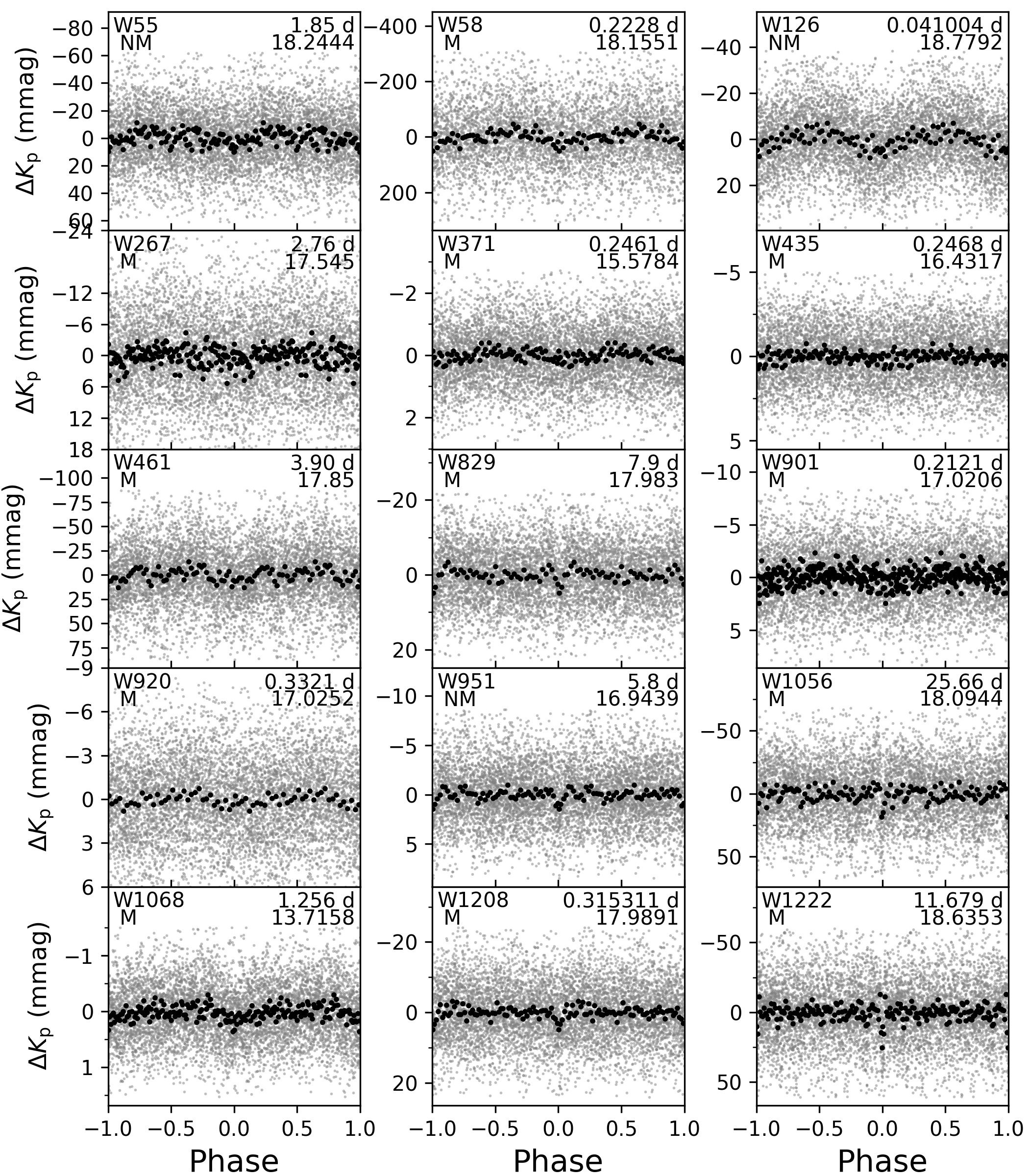
Figure 17: Same as Figure 11, but for suspected variables and for a mixture of cluster members and nonmembers. The first 15 suspected variables are shown in this figure, with the rest of the suspected variables shown in Figures 18, 19, 20, and 21. Cluster membership is indicated below the object identifier in the upper right corner of each panel: “M” means cluster member (specifically, that the cluster membership probability is ${>}$99%), while “NM” means not a cluster member (specifically, that the cluster membership probability is ${<}$1%).

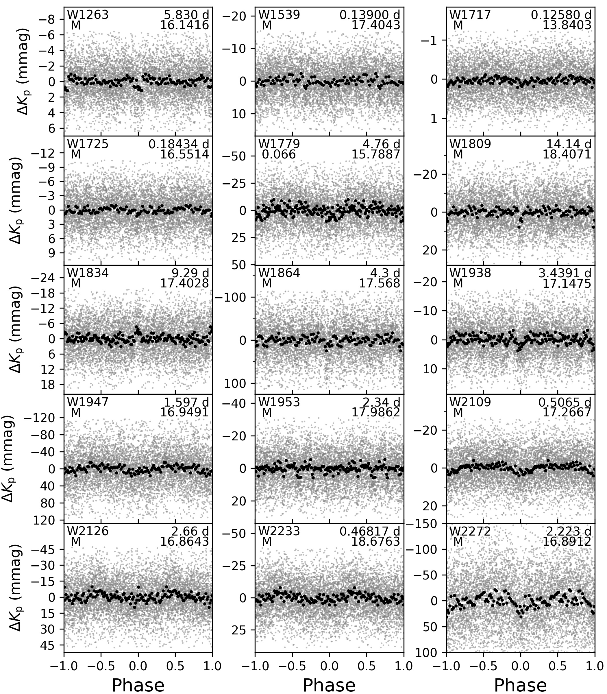
Figure 18: Same as Figure 17, but for additional suspected variables. Instead of indicating “M” or “NM” for W1799’s cluster membership, we record the membership probability since it was not ${<}$1% or ${>}$99%.

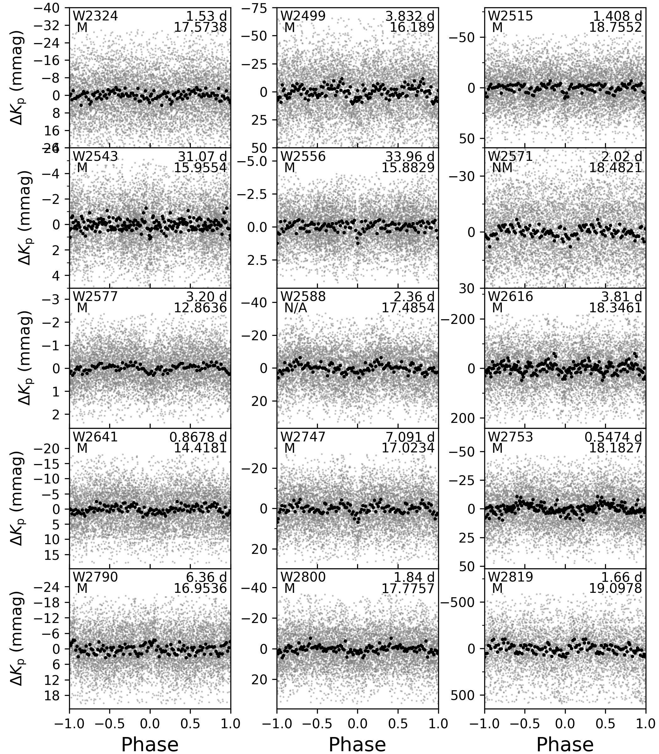
Figure 19: Same as Figure 17, but for additional suspected variables. “N/A” for W2588’s cluster membership status means cluster membership information not available since there are not Gaia DR2 proper motions reported for this object.

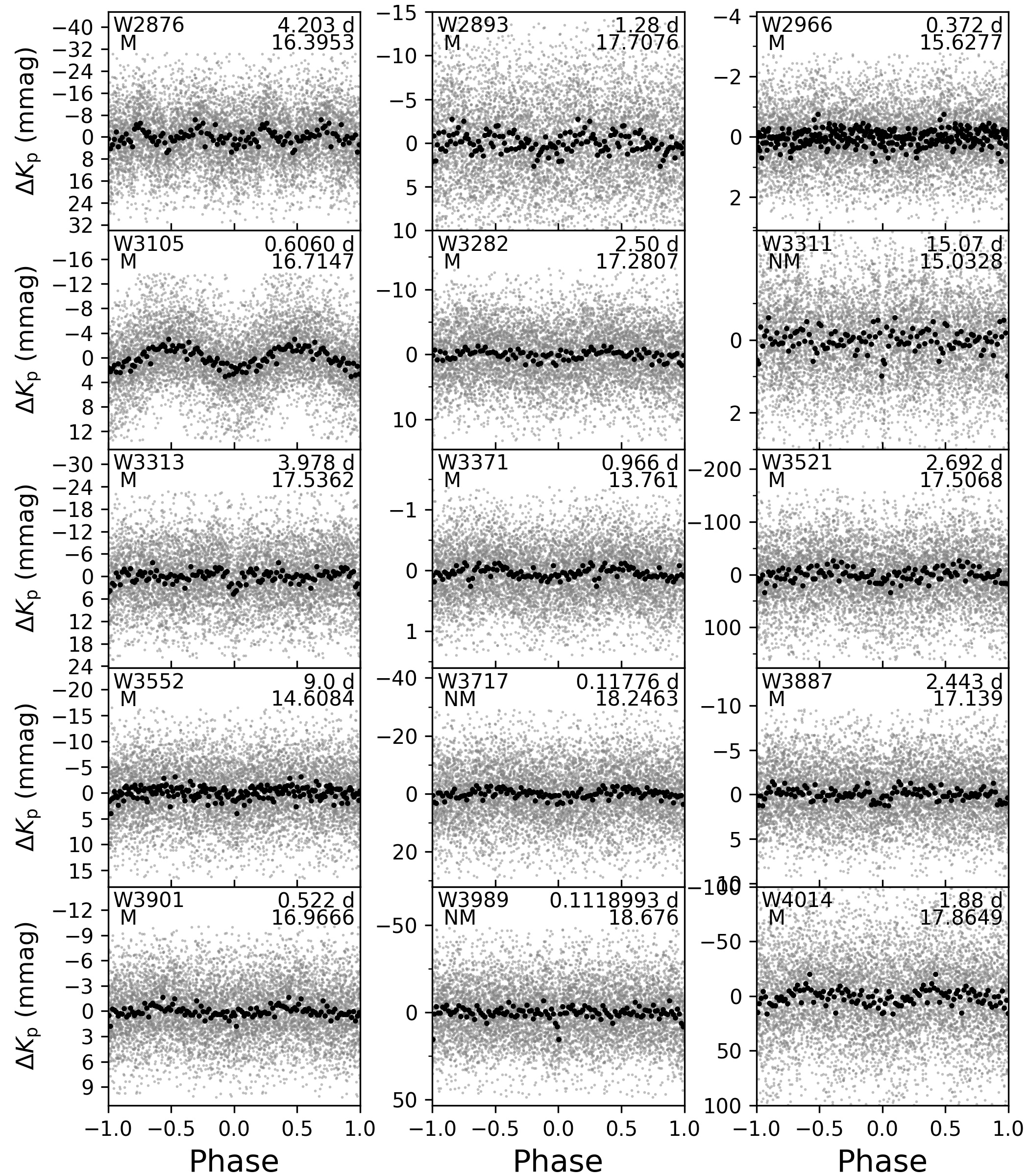
Figure 20: Same as Figure 17, but for additional suspected variables.

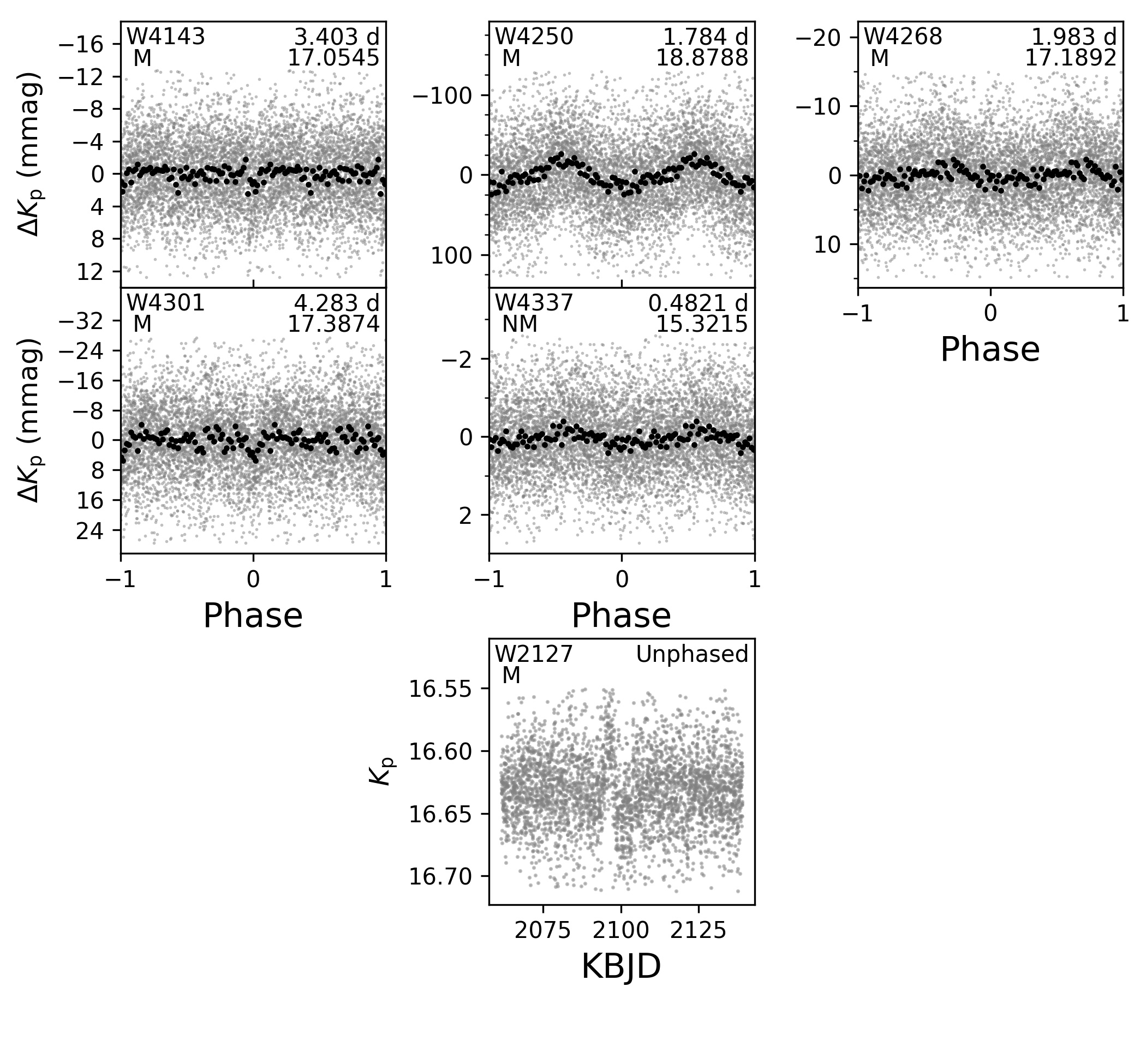
Figure 21: Same as Figure 17, but for additional suspected variables. W2127’s light curve is unphased since only a single event was found.

W1834 in Figure 18 is a cluster member with a ${\sim}$5 mmag box-shaped brightening in the light curve, occurring at a 9.29-day period. We consider the possibility that this is a gravitational self-lens from a neutron star/black hole in a binary with a main sequence star. Figure 1 from Masuda & Hotokezaka (2018) shows that the amplitude and period are consistent with self-lensing from a ${\sim}$10 M_☉ black hole; however, their equation 7 reveals that for a circular orbit such a system would have a signal duration of ${\sim}$1 hour, much shorter than the ${\sim}$20 hours observed. If this is a self-lensing black hole system, it would have to be very eccentric. We would expect ellipsoidal variability in such a case during a pericenter passage, but we do not see anything larger than our ${\sim}$0.1 mag floor in the raw light curves.

Similarly, W2127 in Figure 21 is a cluster member that has a single observed ${\sim}$50 mmag brightening event over a ${\sim}$5-day period. Extrapolating from their figure 1 and again using the equation 7 from Masuda & Hotokezaka (2018) as before, a ${\sim}$10 M_☉ black hole on a ${\sim}$250-day circular orbit would broadly match the observed light curve. Of course, these situations would require an orbital inclination near 90°, which for the wide orbit of W2127 presents something of a fine-tuning problem, as does the large eccentricity needed for W1834. We merely present these as possible scenarios and do not conclude anything on the nature of the variability on these objects.

We list here the reasons we have for marking each of the suspected variables as suspected rather than definite variables.

• W55: Noisy periodogram; low-amplitude phase-folded light curve.

• W58: Many light curve points from second half of campaign are missing due to blending with bright star.

• W126: Very short period, ${\sim}$0.3% away from twice the cadence period.

• W267: Phase-folded light curve has low amplitude.

• W371: Noisy periodogram.

• W435: Noisy periodogram and phase-folded signal has low amplitude.

• W461: Very nearby to W491 and might be blended, W461’s period is a bit more than 14 times the period of W491.

• W829: Small transit depth compared to light curve scatter.

• W901: Noisy periodogram.

• W920: Noisy periodogram and phase-folded signal has low amplitude.

• W951: By-eye judgment call that it is unclear whether this could be a real transit or not.

• W1056: By-eye evaluation makes it unclear whether this could be a real transit or not.

• W1068: Noisy periodogram.

• W1208: Noisy periodogram.

• W1222: Binned-median points show some bright points in transit in addition to the dimmer points filling out the transit.

• W1263: Noisy periodogram.

• W1539: Noisy periodogram and phase-folded signal has low amplitude.

• W1717: Noisy periodogram and phase-folded signal has low amplitude.

• W1725: Phase-folded light curve has low amplitude, ambiguous by eye.

• W1779: Near a saturated star; similar period to W1864, which is also near the same saturated star.

• W1809: Small transit depth compared to light curve scatter.

• W1834: Scatter in anti-transit portion of phase appears to be smaller than the rest of the light curve.

• W1864: Near a saturated star; similar period to W1779, which is also near the same saturated star.

• W1938: Noisy periodogram.

• W1947: In a very crowded area of the image; rich, possibly noisy, periodogram.

• W1953: Possible transit, but depth is not large and not very wide.

• W2109: Periodogram peak similar in amplitude to other periodogram peaks, but phase-folded signal looks like it could be real.

• W2126: Noisy periodogram; phase-folded signal has low amplitude.

• W2127: Signal occurs close to the time the spacecraft’s roll changed directions, producing systematics in other light curves around this time, but this is a stronger signal than those other systematics.

• W2233: Noisy periodogram; looks like an RRab signal and has close to the same period as V9, but they do not quite phase up.

• W2272: Blending with bright object, producing differing noise characteristics in second half of data relative to first half, may be producing some kind of unique systematic.

• W2324: Noisy periodogram; period matches W1189 and is 180° out of phase, but it is over 55 pixels away.

• W2499: Noisy periodogram

• W2515: Noisy periodogram.

• W2543: Transit not very deep compared to noise.

• W2556: Only two transits observed.

• W2571: Noisy periodogram; strange shape to periodogram peak.

• W2577: A bright star blended with another bright star for which we do not have light curves since they are not Gaia DR1 sources, thus unsure whether this is the source of variability (though very likely it is).

• W2588: Noisy periodogram.

• W2616: Noise characteristics changed halfway through campaign.

• W2641: Noisy periodogram.

• W2747: Low-amplitude transit signal.

• W2753: Based on period, it might be a transformed blend of V29.

• W2790: Phase-folded light curve has low amplitude.

• W2800: Phase-folded light curve has low amplitude.

• W2819: Maybe a transit present, but differing noise characteristics in second half of data relative to first half may be producing some kind of unique systematic.

• W2876: Noise characteristics change slightly halfway through campaign; noisy periodogram.

• W2893: Noisy periodogram.

• W2966: Phase-folded light curve has low amplitude.

• W3105: Six pixels away from and similar variability to V27, but does not phase up. However, we have seen our light curve processing transform blended RRAB signals into sinusoidal signals with slightly different periods.

• W3125: Noisy periodogram.

• W3282: Phase-folded light curve of particularly small amplitude.

• W3311: Noisy periodogram.

• W3313: Low-amplitude transit signal.

• W3371: Phase-folded light curve has low amplitude.

• W3521: Noisy periodogram.

• W3552: Noisy periodogram.

• W3717: Noisy periodogram; phase-folded light curve has low amplitude.

• W3887: Small transit depth compared to light curve scatter.

• W3901: Low-amplitude signal. Period matches V29, but does not phase up, and is over 120 pixels away.

• W3989: Noisy periodogram.

• W4014: Noisy periodogram; phase-folded signal has low amplitude.

• W4143: Small transit depth compared to light curve scatter.

• W4250: Near to a bright star that was in the edge region. We do not have the light curve for the bright star to see if this signal is a blend.

• W4268: Period falls within the 1.95-day systematic range, but we still decided to keep as a suspected variable based on signal strength.

• W4301: Noisy periodogram.

• W4337: Noisy periodogram; phase-folded light curve has low amplitude.

References

- Alard & Lupton (1998) Alard, C., & Lupton, R. H. 1998, ApJ, 503, 325, doi: 10.1086/305984
- Astropy Collaboration et al. (2018) Astropy Collaboration, Price-Whelan, A. M., Sipőcz, B. M., et al. 2018, AJ, 156, 123, doi: 10.3847/1538-3881/aabc4f
- Barentsen (2016) Barentsen, G. 2016, barentsen/k2mosaic: v2.0.0, Zenodo, doi: 10.5281/zenodo.167343. https://zenodo.org/record/167343#.W9nI15y1thE
- Barentsen et al. (2018) Barentsen, G., Hedges, C., Saunders, N., et al. 2018, arXiv e-prints, arXiv:1810.12554. https://arxiv.org/abs/1810.12554
- Bassa et al. (2004) Bassa, C., Pooley, D., Homer, L., et al. 2004, ApJ, 609, 755, doi: 10.1086/421259
- Bedin et al. (2009) Bedin, L. R., Salaris, M., Piotto, G., et al. 2009, ApJ, 697, 965, doi: 10.1088/0004-637X/697/2/965
- Bhatti et al. (2017) Bhatti, W., Bouma, L. G., & Wallace, J. 2017, astrobase, Zenodo, doi: 10.5281/zenodo.1011188. https://doi.org/10.5281/zenodo.1011188
- Braga et al. (2015) Braga, V., Dall’Ora, M., Bono, G., et al. 2015, ApJ, 799, 165
- Clement et al. (2001) Clement, C. M., Muzzin, A., Dufton, Q., et al. 2001, AJ, 122, 2587, doi: 10.1086/323719
- Clementini et al. (1994) Clementini, G., Merighi, R., Pasquini, L., Cacciari, C., & Gouiffes, C. 1994, MNRAS, 267, 83, doi: 10.1093/mnras/267.1.83
- Eggen (1972) Eggen, O. J. 1972, ApJ, 172, 639, doi: 10.1086/151383
- Evans et al. (2018) Evans, D. W., Riello, M., De Angeli, F., et al. 2018, A&A, 616, A4, doi: 10.1051/0004-6361/201832756
- Gaia Collaboration et al. (2016a) Gaia Collaboration, Brown, A. G. A., Vallenari, A., et al. 2016a, A&A, 595, A2, doi: 10.1051/0004-6361/201629512
- Gaia Collaboration et al. (2016b) Gaia Collaboration, Prusti, T., de Bruijne, J. H. J., et al. 2016b, A&A, 595, A1, doi: 10.1051/0004-6361/201629272
- Gaia Collaboration et al. (2018) Gaia Collaboration, Brown, A. G. A., Vallenari, A., et al. 2018, A&A, 616, A1, doi: 10.1051/0004-6361/201833051
- Gilliland et al. (2000) Gilliland, R. L., Brown, T. M., Guhathakurta, P., et al. 2000, ApJ, 545, L47, doi: 10.1086/317334
- Harris (1996) Harris, W. E. 1996, AJ, 112, 1487
- Hartman & Bakos (2016) Hartman, J. D., & Bakos, G. Á. 2016, Astronomy and Computing, 17, 1, doi: 10.1016/j.ascom.2016.05.006
- Howell et al. (2014) Howell, S. B., Sobeck, C., Haas, M., et al. 2014, PASP, 126, 398, doi: 10.1086/676406
- Hunter (2007) Hunter, J. D. 2007, Computing In Science & Engineering, 9, 90
- Jones et al. (2001) Jones, E., Oliphant, T., Peterson, P., et al. 2001, SciPy: Open source scientific tools for Python. http://www.scipy.org/
- Kaluzny et al. (1997) Kaluzny, J., Thompson, I. B., & Krzeminski, W. 1997, AJ, 113, 2219, doi: 10.1086/118432
- Kaluzny et al. (2013a) Kaluzny, J., Thompson, I. B., Rozyczka, M., & Krzeminski, W. 2013a, Acta Astron., 63, 181. https://arxiv.org/abs/1306.2457
- Kaluzny et al. (2013b) Kaluzny, J., Thompson, I. B., Rozyczka, M., et al. 2013b, AJ, 145, 43, doi: 10.1088/0004-6256/145/2/43
- Kovács et al. (2005) Kovács, G., Bakos, G., & Noyes, R. W. 2005, MNRAS, 356, 557, doi: 10.1111/j.1365-2966.2004.08479.x
- Kovács et al. (2002) Kovács, G., Zucker, S., & Mazeh, T. 2002, A&A, 391, 369, doi: 10.1051/0004-6361:20020802
- Kuehn et al. (2017) Kuehn, C. A., Moskalik, P., & Drury, J. A. 2017, in Seismology of the Sun and the Distant Stars - Using Today’s Successes to Prepare the Future - TASC2 & KASC9 Workshop - SPACEINN & HELAS8 Conference, Azores Islands, Portugal, Edited by Monteiro, M.J.P.F.G.; Cunha, M.S.; Ferreira, J.M.T.S.; EPJ Web of Conferences, Volume 160, id.04011, Vol. 160, 04011
- LaCourse et al. (2015) LaCourse, D. M., Jek, K. J., Jacobs, T. L., et al. 2015, MNRAS, 452, 3561, doi: 10.1093/mnras/stv1475
- Leavitt & Pickering (1904) Leavitt, H. S., & Pickering, E. C. 1904, Harvard College Observatory Circular, 90, 1
- Libralato et al. (2016a) Libralato, M., Bedin, L. R., Nardiello, D., & Piotto, G. 2016a, MNRAS, 456, 1137, doi: 10.1093/mnras/stv2628
- Libralato et al. (2016b) Libralato, M., Nardiello, D., Bedin, L. R., et al. 2016b, MNRAS, 463, 1780, doi: 10.1093/mnras/stw1932
- Lindegren et al. (2016) Lindegren, L., Lammers, U., Bastian, U., et al. 2016, A&A, 595, A4, doi: 10.1051/0004-6361/201628714
- Lindegren et al. (2018) Lindegren, L., Hernández, J., Bombrun, A., et al. 2018, A&A, 616, A2, doi: 10.1051/0004-6361/201832727
- Lomb (1976) Lomb, N. R. 1976, Ap&SS, 39, 447, doi: 10.1007/BF00648343
- Masuda & Hotokezaka (2018) Masuda, K., & Hotokezaka, K. 2018, arXiv e-prints, arXiv:1808.10856. https://arxiv.org/abs/1808.10856
- Miglio et al. (2016) Miglio, A., Chaplin, W. J., Brogaard, K., et al. 2016, MNRAS, 461, 760, doi: 10.1093/mnras/stw1555
- Nardiello et al. (2016) Nardiello, D., Libralato, M., Bedin, L. R., et al. 2016, MNRAS, 463, 1831, doi: 10.1093/mnras/stw2169
- Nascimbeni et al. (2012) Nascimbeni, V., Bedin, L. R., Piotto, G., De Marchi, F., & Rich, R. M. 2012, A&A, 541, A144, doi: 10.1051/0004-6361/201118655
- Neeley et al. (2015) Neeley, J., Marengo, M., Bono, G., et al. 2015, The Astrophysical Journal, 808, 11
- Oliphant (2006) Oliphant, T. 2006, Guide to NumPy (Trelgol Publishing). http://www.tramy.us/numpybook.pdf
- Pál (2012) Pál, A. 2012, MNRAS, 421, 1825, doi: 10.1111/j.1365-2966.2011.19813.x
- Pedregosa et al. (2011) Pedregosa, F., Varoquaux, G., Gramfort, A., et al. 2011, Journal of Machine Learning Research, 12, 2825
- Ricker et al. (2015) Ricker, G. R., Winn, J. N., Vanderspek, R., et al. 2015, Journal of Astronomical Telescopes, Instruments, and Systems, 1, 014003, doi: 10.1117/1.JATIS.1.1.014003
- Riello et al. (2018) Riello, M., De Angeli, F., Evans, D. W., et al. 2018, A&A, 616, A3, doi: 10.1051/0004-6361/201832712
- Russell (1948) Russell, H. N. 1948, The Royal Road of Eclipses, Vol. 7 (Harvard Observatory Monographs), 181
- Safonova et al. (2016) Safonova, M., Mkrtichian, D., Hasan, P., et al. 2016, AJ, 151, 27, doi: 10.3847/0004-6256/151/2/27
- Samus et al. (2017) Samus, N. N., Kazarovets, E. V., Durlevich, O. V., Kireeva, N. N., & Pastukhova, E. N. 2017, Astronomy Reports, 61, 80, doi: 10.1134/S1063772917010085
- Scargle (1982) Scargle, J. D. 1982, ApJ, 263, 835, doi: 10.1086/160554
- Soares-Furtado et al. (2017) Soares-Furtado, M., Hartman, J. D., Bakos, G. Á., et al. 2017, PASP, 129, 044501, doi: 10.1088/1538-3873/aa5c7c
- Stellingwerf (1978) Stellingwerf, R. F. 1978, ApJ, 224, 953, doi: 10.1086/156444
- Stetson et al. (2014) Stetson, P. B., Braga, V. F., Dall’Ora, M., et al. 2014, PASP, 126, 521
- van Leeuwen et al. (2017) van Leeuwen, F., Evans, D. W., De Angeli, F., et al. 2017, A&A, 599, A32, doi: 10.1051/0004-6361/201630064
- VandenBerg et al. (2013) VandenBerg, D. A., Brogaard, K., Leaman, R., & Casagrande, L. 2013, ApJ, 775, 134, doi: 10.1088/0004-637X/775/2/134
- Vanderburg & Johnson (2014) Vanderburg, A., & Johnson, J. A. 2014, PASP, 126, 948, doi: 10.1086/678764
- Vanderburg et al. (2016) Vanderburg, A., Latham, D. W., Buchhave, L. A., et al. 2016, ApJS, 222, 14
- Verbunt (2001) Verbunt, F. 2001, A&A, 368, 137, doi: 10.1051/0004-6361:20000469
- Wallace (2018a) Wallace, J. 2018a, M4_pm_membership: Version 1.0, Zenodo, doi: 10.5281/zenodo.1488302. https://doi.org/10.5281/zenodo.1488302
- Wallace & Hoffman (2019) Wallace, J., & Hoffman, J. 2019, simple_deblend, Zenodo, doi: 10.5281/zenodo.3248998. https://doi.org/10.5281/zenodo.3248998
- Wallace (2018b) Wallace, J. J. 2018b, Research Notes of the AAS, 2, 213
- Wallace et al. (2019a) Wallace, J. J., Hartman, J. D., Bakos, G. Á., & Bhatti, W. 2019a, ApJ, 870, L7, doi: 10.3847/2041-8213/aaf8ac
- Wallace et al. (2019b) —. 2019b, Light Curves from a Search for Variable Stars in the Globular Cluster M4 with K2, DataSpace at Princeton University. http://arks.princeton.edu/ark:/88435/dsp01h415pd368
- Watson et al. (2017) Watson, C., Henden, A. A., & Price, A. 2017, VizieR Online Data Catalog, 1
- Weldrake et al. (2008) Weldrake, D. T. F., Sackett, P. D., & Bridges, T. J. 2008, ApJ, 674, 1117, doi: 10.1086/524917
- Weldrake et al. (2005) Weldrake, D. T. F., Sackett, P. D., Bridges, T. J., & Freeman, K. C. 2005, ApJ, 620, 1043, doi: 10.1086/427258
- Yao et al. (2006a) Yao, B.-A., Sheng, C.-J., & Shi, H.-M. 2006a, Ap&SS, 302, 241, doi: 10.1007/s10509-006-9040-0
- Yao et al. (2006b) Yao, B.-a., Sheng, C.-j., Zhang, C.-s., Hu, H.-m., & Lin, Q. 2006b, Chinese Astron. Astrophys., 30, 351, doi: 10.1016/j.chinastron.2006.10.001
- Yao et al. (2007) Yao, B. A., Sheng, C. J., Zhang, C. S., Hu, H. M., & Lin, Q. 2007, Acta Astronomica Sinica, 48, 18
- Yao & Tong (1989) Yao, B.-A., & Tong, J.-H. 1989, Information Bulletin on Variable Stars, 3334, 1
- Yao et al. (1988) Yao, B. A., Tong, J. H., & Zhang, C. S. 1988, Acta Astronomica Sinica, 29, 243
- Yao et al. (1981a) Yao, B. A., Yin, J. S., & Guo, Z. H. 1981a, Acta Astrophysica Sinica, 1, 311
- Yao et al. (1981b) Yao, B.-a., Yin, J.-s., & Guo, Z.-h. 1981b, Chinese Astron. Astrophys., 5, 476, doi: 10.1016/0275-1062(81)90015-1
- Zechmeister & Kürster (2009) Zechmeister, M., & Kürster, M. 2009, A&A, 496, 577, doi: 10.1051/0004-6361:200811296
- Zhu et al. (2017) Zhu, W., Huang, C. X., Udalski, A., et al. 2017, PASP, 129, 104501, doi: 10.1088/1538-3873/aa7dd7