Finite Pulse Waves for Efficient Suppression of Evolving Mesoscale Dendrites in Rechargeable Batteries

Abstract

The ramified and stochastic evolution of dendritic microstructures has been a major issue on the safety and longevity of rechargeable batteries, particularly for the utilization high-energy metallic electrodes. We analytically develop criteria for the pulse characteristics leading to the effective halting of the ramified electrodeposits grown during extensive time scales beyond inter-ionic collisions. Our framework is based on the competitive interplay between diffusion and electromigration and tracks the gradient of ionic concentration throughout the entire cycle of pulse-rest as a critical measure for heterogeneous evolution. In particular, the framework incorporates the Brownian motion of the ions and investigates the role of the geometry of the electrodeposition interface. Our novel experimental observations verify the analytical developments, where the the dimension-free developments allows the application to the electrochemical systems of various scales.

Keywords: Random Walk, Pulse Charge, Dendritic Evolution, Concentration Gradient.

1 Introduction

Metallic anodes such as lithium, sodium and zinc are arguably highly attractive candidates for use in high-energy and high-power density rechargeable batteries.[1, 2, 3] In particular, lithium metal possess the lowest density and smallest ionic radius which provides a very high gravimetric energy density and possesses the highest electropositivity ($E^{0}=-3.04V$ vs SHE) that likely provides the highest possible voltage, making it suitable for high-power applications such as electric vehicles. ($\rho=0.53\leavevmode\nobreak\ g.cm^{-3}$).[4, 5] During the charging, the fast-pace formation of microstructures with relatively low surface energy from Brownian dynamics, leads to the branched evolution with high surface to volume ratio.[6] The quickening tree-like morphologies could occupy a large volume, possibly reach the counter-electrode and short the cell. Additionally, the can also dissolve from their thinner necks during subsequent discharge period. Such a formation-dissolution cycle is particularly prominent for the metal electrodes due to lack of intercalation.[7] Previous studies have investigated various factors on dendritic formation such as current density,[8] electrode surface roughness [9, 10, 11], impurities [12, 13], solvent and electrolyte chemical composition [14, 15], electrolyte concentration [16], utilization of powder electrodes [17] and adhesive polymers[18], temperature [19], guiding scaffolds [20, 21], capillary pressure [22], cathode morphology [23] and mechanics [24, 25]. Some of conventional characterization techniques used include NMR [26] and MRI. [27] Recent studies also have shown the necessity of stability of solid electrolyte interphase (i.e. SEI) layer for controlling the nucleation and growth of the branched medium. [28, 29]

Earlier model of dendrites had focused on the electric field and space charge as the main responsible mechanism [30] while the later models focused on ionic concentration causing the diffusion limited aggregation (DLA). [31, 32, 33] Both mechanisms are part of the electrochemical potential [34, 35], indicating that each could be dominant depending on the localizations of the electric potential or ionic concentration within the medium. Nevertheless, their interplay has been explored rarely, especially in continuum scale and realistic time intervals, matching scales of the experimental time and space.

Dendrites instigation is rooted in the non-uniformity of electrode surface morphology at the atomic scale combined with Brownian ionic motion during electrodeposition. Any asperity in the surface provides a sharp electric field that attracts the upcoming ions as a deposition sink. Indeed the closeness of a convex surface to the counter electrode, as the source of ionic release, is another contributing factor. In fact, the same mechanism is responsible for the further semi-exponential growth of dendrites in any scale. During each pulse period the ions accumulate at the dendrites tips (unfavorable) due to high electric field in convex geometry and during each subsequent rest period the ions tend to diffuse away to other less concentrated regions (favorable). The relaxation of ionic concentration during the idle period provides a useful mechanism to achieve uniform deposition and growth during the subsequent pulse interval. Such dynamics typically occurs within the double layer (or stern layer [36]) which is relatively small and comparable to the Debye length. In high charge rates, the ionic concentration is depleted and concentration on the depletion reaches zero [37]; Nonetheless, our continuum-level study extends to larger scale, beyond the double layer region. [38]

Pulse method has been qualitatively proved as a powerful approach for the prevention of dendrites [39], which has previously been utilized for uniform electroplating.[40] In the preceding publication we have experimentally found that the optimum rest period correlates well with the relaxation time of the double layer for the blocking electrodes [41] which is interpreted as the RC time of the electrochemical system. [42] We have explained qualitatively how relatively longer pulse periods with identical duty cycles $D$ (or idle ratio $\gamma$) will lead to longer and more quickening growing dendrites. We developed coarse grained computationally affordable algorithm that allowed us reach to the experimental time scale ($ms$). Additionally, in the recent theoretical work we indicated that there is an analytical criterion for the optimal inhibition of growing dendrites. [43]

In this paper, we elaborate further in the range of acceptable duty cycle $\mathbf{D}$ for suppression of stochastically-grown dendrites and we develop new insight for the effective rest period on the curved boundary. Subsequently we carry out experimental investigation to verify our analytical developments on the pulse parameters. We perform dimensional analysis to set our formulation applicable to the large range of electrochemical devices.

2 Methodology

The pulse charging in its simplest form consists of trains of square active period $t_{ON}$ , followed by a square rest interval $t_{OFF}$ in terms of current $I$ or voltage $V$ as shown in Figure 2. The period $P=t_{ON}+t_{OFF}$ is the time lapse of a full cycle. Hence the pulse frequency $f$ is:

$$f=\frac{1}{t_{ON}+t_{OFF}}$$ (1)

and the duty cycle $\mathbf{D}$ represents the fraction of time in the period $P$ that the pulse is active :

$$\mathbf{D}=ft_{ON}$$ (2)

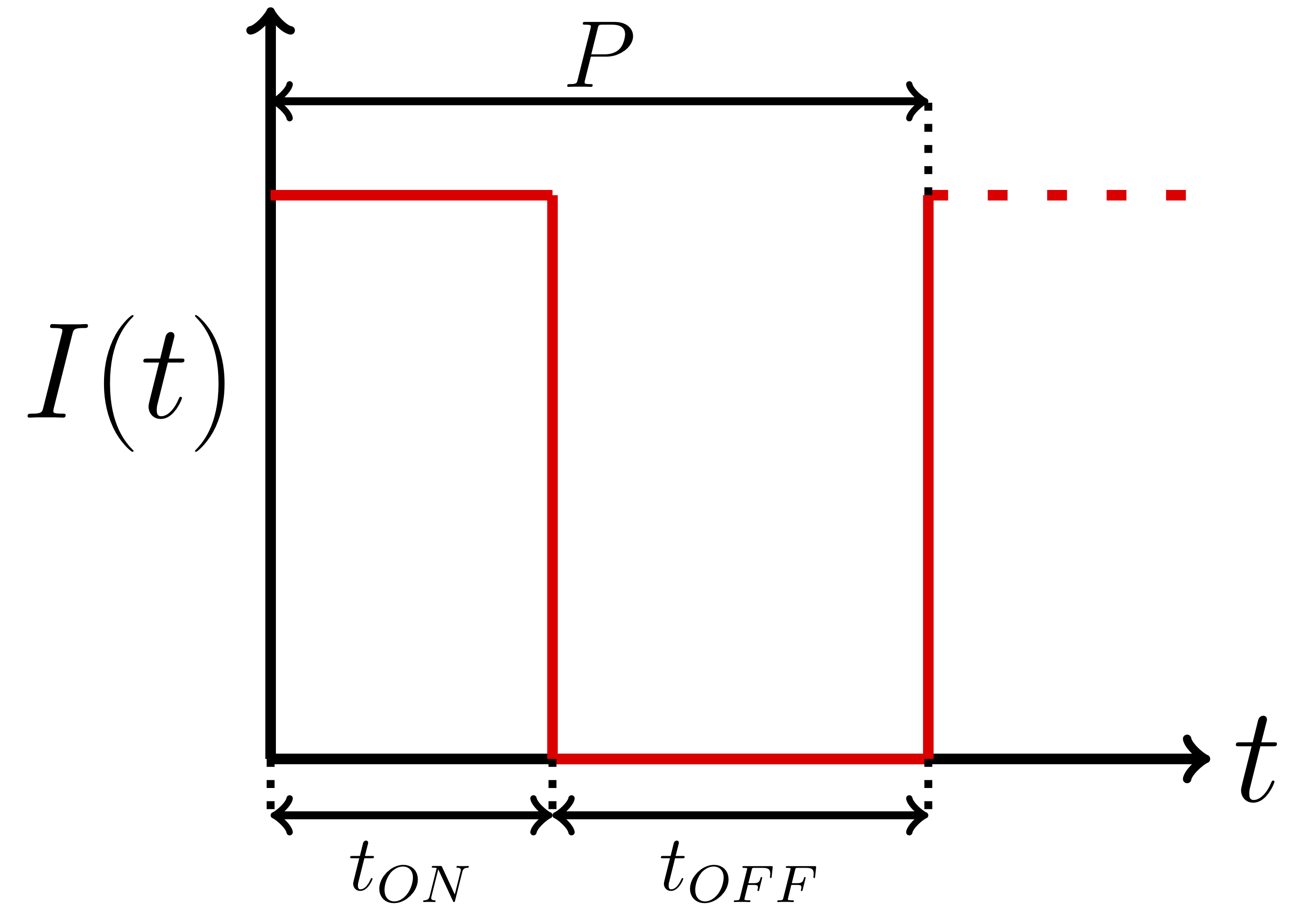
Figure 1: Square pulse wave.

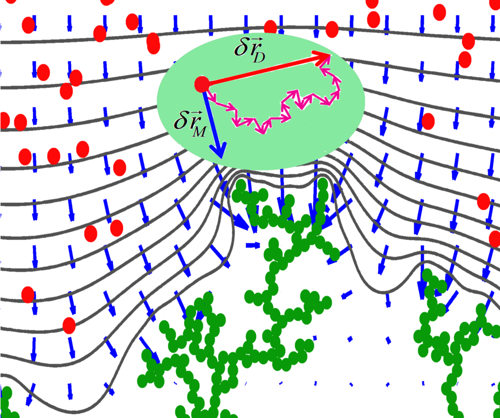
Figure 2: The transport elements in the coarse scale of time and space.

The electrochemical flux is generated either from the gradients of concentration ($\nabla C$) or electric potential ($\nabla\phi$). In the ionic scale, the regions of higher concentration tend to collide and repel more and, given enough time, diffuse to lower concentration zones, following Brownian motion. In the continuum scale, such inter-collisions could be added-up and be represented by the diffusion length $\delta\vec{\textbf{r}}_{D}$ as: [41]

$$\delta\vec{\textbf{r}}_{D}=\sqrt{2D^{+}\delta t}\text{ }\hat{\textbf{g}}$$ (3)

where $\vec{\textbf{r}}_{D}$ is diffusion displacement of individual ion, $D^{+}$ is the cationic diffusion coefficient in the electrolyte, $\delta t$ is the coarse time interval, and $\hat{\textbf{g}}$ is a normalized vector in random direction, representing the Brownian dynamics. The diffusion length represents the average progress of a diffusive wave in a given time, obtained directly from the diffusion equation. [44]

On the other hand, ions tend to acquire drift velocity in the electrolyte medium when exposed to electric field and during the given time $\delta t$ their progress $\delta\vec{\textbf{r}}_{M}$ is given as:

$$\delta\vec{\textbf{r}}_{M}=\mu^{+}\vec{\textbf{E}}\delta t$$ (4)

where $\mu^{+}$ is the mobility of cations in electrolyte, $\vec{\textbf{E}}$ is the local electric field, which is the gradient of electric potential ($\vec{\textbf{E}}=-\nabla\phi$ ). Therefore the total effective displacement $\delta\vec{\textbf{r}}$ with neglecting convection would be:

$$\delta\vec{\textbf{r}}=\delta\vec{\textbf{r}}_{D}+\delta\vec{\textbf{r}}_{M}$$ (5)

as represented in the Figure 2. Based on the Equations 1 and 2, defining two parameters will uniquely characterize the pulse charge. We choose them as duty cycle $\mathbf{D}$ (section 2.1) and the relaxation (i.e. rest) period $t_{OFF}$ (section 2.2) as follows next.

2.1 Optimum Duty cycle

The vector sum in Equation 5 indicates that the diffusion, as a random walk, can either contribute to electro-migration or prevents its progress, depending on the local orientation of the gradients of concentration and electric potential $\{\nabla C,\nabla\phi\}$. From Figure 2 it is visually obvious that the sum of individual diffusional displacements after after the $n$ number of collisions within the time interval $\delta t$ always is larger (or equal to) than the on-step displacement of diffusion front during the entire time coarse time interval ${\displaystyle\delta t=\sum_{i=1}^{n}\delta t_{i}}$ as:

$$\sum_{i=1}^{n}\sqrt{2D^{+}\delta t_{i}}\geq\sqrt{2D^{+}\sum_{i=1}^{n}\delta t_{i}}$$ (6)

We verify the Equation 6 by induction. The equation is obvious for value of $n:=1$, therefore we need to prove that if Equation 6 is true for the $n:=k$, then it should be true for $n:=k+1$.

$$\sum_{i=1}^{k+1}\sqrt{2D^{+}\delta t_{i}}\geq\sqrt{2D^{+}\sum_{i=1}^{k+1}\delta t_{i}}$$ (7)

Assuming that $\delta t_{i}=\delta t$ (i.e. equal segmentation) the inequality 7 can be broken down as:

$$\sum_{i=1}^{k}\sqrt{2D^{+}\delta t_{i}}+\sqrt{2D^{+}\delta t}\geq\sqrt{2D^{+}\sum_{i=1}^{k}\delta t_{i}+2D^{+}\delta t}$$

Taking to the power 2, with simplification, we get the following:

$$2k(k+1)D^{+}\delta t\text{ }\geq 0\text{ }\checkmark$$ (8)

which means that Equation 7 is true for any consecutive value of $k\rightarrow k+1$ and therefore indefinitely for any $k\in\mathbb{N}$. In fact, Equation 6 represents the extended version of triangle inequality in terms of mean-square diffusion distance. [46] During each pulse period $t_{ON}$, both diffusion and migration are active for the ionic displacements. Therefore, depending on their individual orientation they can help or hurt each other. Thus the range of ionic displacement $|\delta\vec{\textbf{r}}|_{ON}$ in the pulse period is obtained as:

$$\mu^{+}\vec{\textbf{E}}\delta t-\sum_{i=1}^{n}\sqrt{2D^{+}\delta t_{i}}\leq|\delta\vec{\textbf{r}}|_{ON}\leq\mu^{+}\vec{\textbf{E}}\delta t+\sum_{i=1}^{n}\sqrt{2D^{+}\delta t_{i}}$$ (9)

where $\mu^{+}$ and $D^{+}$ are the mobility and the diffusion coefficient of local ions and $\vec{\textbf{E}}$ is the local electric field respectively. For the Equation 9 to be valid, considering Equation 6, one must have:

$$\mu^{+}\vec{\textbf{E}}\delta t-\sqrt{2D^{+}\delta t}\leq|\delta\vec{\textbf{r}}|_{ON}\leq\mu^{+}\vec{\textbf{E}}\delta t+\sqrt{2D^{+}\delta t}$$ (10)

Such a random walk is succeeded with the idle period $t_{OFF}$ where the the diffusion is the sole drive for the relaxation. In order to have uniform electrodeposition, the average progress of diffusive wave in the rest period $t_{OFF}$ has to be competitive enough with the pulse interval $t_{ON}$, hence:

$$\sqrt{2D^{+}t_{OFF}}\geq\mu^{+}\vec{\textbf{E}}t_{ON}\pm\sqrt{2D^{+}t_{ON}}$$ (11)

Without further look into Equation 11, it is obvious that $t_{OFF}\geq t_{ON}$. For simplification, we define the idle ratio as $\gamma:={\displaystyle\frac{t_{OFF}}{t_{ON}}}$ and further elaboration leads to:

$$\gamma\pm 2\sqrt{\gamma}+1-\frac{\mu^{+}|\vec{\textbf{E}}|^{2}}{2RT}t_{ON}\geq 0$$ (12)

The solution to the Equation 12 represent the idle ratio for effective fading of as:

$$\gamma\geq\left(1\pm|\vec{\textbf{E}}|\sqrt{\frac{2\mu^{+}t_{ON}}{RT}}\right)^{2}$$ (13)

and the duty cycle $\mathbf{D}$ in term of the idle ratio $\gamma$ is obtained as:

$$\mathbf{D}=\frac{t_{ON}}{t_{ON}+t_{OFF}}=\frac{1}{1+\gamma}$$ (14)

Noting the Einstein relationship ($D^{+}=\mu^{+}RT$), the range of acceptable duty cycle $\mathbf{D}$ would be:

$$\mathbf{D}\leq\frac{1}{\left(1+{\displaystyle\frac{|\vec{\textbf{E}}|}{RT}}\sqrt{{\displaystyle\frac{D^{+}}{2f}}}\right)^{2}\pm 1}$$ (15)

2.2 Optimum relaxation

The dendritic tip in fact attracts a significant number of ions due to high electric field. Given sufficient time, such ionic concentration profile can disappear in the vicinity of curved electrodeposits during subsequent idle period. Therefore, the relaxation of concentration plays a key role for preventing dendritic deposition. In fact the oscillation of the concentration gradient repeatedly occurs during each pulse-rest period.[37] Herein, we address a time measure for concentration relaxation in the continuum scale with the curved boundary rising from the tip of growing dendrites.

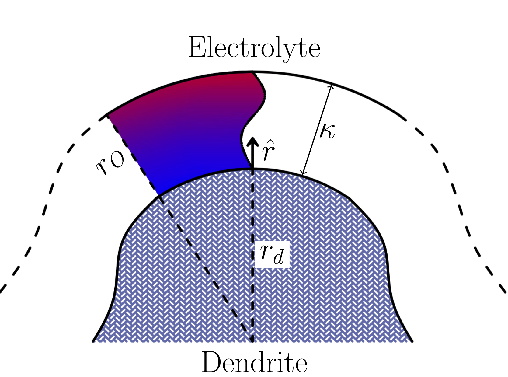
Figure 3: The curved dendrites with the concentration gradient the vicinity of surface.

The schematics of the convex dendrites is shown in Figure 3 with the surrounding double layer of thickness of $\kappa$ and the outer electro-neutral medium. The color gradient represents the concentration profile in the double-layer region. The radius of curvature $r_{d}$ could vary from atomic radius ($r_{d}\approx r_{Li^{+}}\to 10^{-9}m$)[41] to nearly flat surfaces ($r_{d}\rightarrow\infty$). Such a wide range makes orders-of-magnitude of difference in the electric field and concentration dynamics, making it critical factor to consider. We define the normalized dendrite radial distance $\hat{r}\in[0,1]$ from the tip as:

$$\hat{r}:=\frac{r-r_{d}}{\kappa}$$ (16)

where $r$ is the center of curvature. Subsequently we can define the normalized concentration $\hat{C}\in[0,1]$ as:

$$\hat{C}(\hat{r}):=\frac{C(\hat{r})}{C_{\infty}}$$ (17)

where the index $\infty$ represent the ambient electro-neutral medium. The typical diffusion equation in polar 2D coordinates is defined as:

$$\frac{\partial C}{\partial t} =\mathbf{\nabla}.(D^{+}\nabla C)$$ (18)

$$=\left(\frac{\partial}{\partial r}+\frac{1}{r}\frac{\partial}{\partial\theta}\right).\left(D(\frac{\partial C}{\partial r}+\frac{1}{r}\frac{\partial C}{\partial\theta})\right)$$

$$=D^{+}\left(\frac{\partial^{2}C}{\partial r^{2}}+\frac{1}{r}\frac{\partial C}{\partial r}\right)$$

Using the chain derivative and noting Equation 17 we get:

$$\frac{\partial C}{\partial t}=\frac{\partial C}{\partial\hat{C}}\frac{\partial\hat{C}}{\partial t}=C_{\infty}\frac{\partial\hat{C}}{\partial t}$$ (19)

Respectively for the radial space derivative is obtained, considering Equation 16 as:

$$\frac{\partial C}{\partial r}=\frac{\partial C}{\partial\hat{C}}\frac{\partial\hat{C}}{\partial\hat{r}}\frac{\partial\hat{r}}{\partial r}=\frac{C_{\infty}}{\kappa}\frac{\partial\hat{C}}{\partial\hat{r}}$$ (20)

The second radial derivative is respectively obtained as:

$$\frac{\partial^{2}C}{\partial r^{2}} =\frac{\partial}{\partial r}\left(\frac{\partial C}{\partial r}\right)=\frac{\partial}{\partial r}\left(\frac{C_{\infty}}{\kappa}\frac{\partial\hat{C}}{\partial\hat{r}}\right)$$ (21)

$$=\frac{C_{\infty}}{\kappa}\frac{\partial}{\partial\hat{r}}\left(\frac{\partial\hat{C}}{\partial\hat{r}}\right)\frac{\partial\hat{r}}{\partial r}=\frac{C_{\infty}}{\kappa^{2}}\frac{\partial^{2}\hat{C}}{\partial\hat{r}^{2}}$$

Therefore, replacing all the obtained terms from Equations 19, 20 and 21 into Equations 18 and simplification leads to:

$$\kappa^{2}\frac{\partial\hat{C}}{\partial t}=D^{+}\left(\frac{\partial^{2}\hat{C}}{\partial\hat{r}^{2}}+\frac{\kappa}{r_{d}+\kappa\hat{r}}\frac{\partial\hat{C}}{\partial\hat{r}}\right)$$ (22)

Regarding the boundary conditions, while the concentration is depleted in the double layer, in the outer boundary ($\hat{r}\rightarrow 1$) it remains as the ambient value $C_{\infty}$ :

$$\hat{C}(1,t)=1$$ (23)

During the charge period, a constant reduction ionic flux $j$ is fed to the dendrite and respectively during the idle period there will be no reaction since the dendrites will not accept any ions. Therefore:

$$\left\{\begin{array}[]{ll}\cfrac{\partial\hat{C}}{\partial\hat{r}}(0,t)&={\displaystyle\frac{\kappa}{C_{\infty}}\frac{\partial C}{\partial r}=-\frac{\kappa j}{C_{\infty}D^{+}}\text{$\hskip 25.6073pt\text{Pulse}$}}\\ \cfrac{\partial\hat{C}}{\partial\hat{r}}(0,t)&=0\hskip 109.54327pt\text{Rest}\end{array}\right.$$ (24)

The Equation 22 can be solved numerically using a finite difference method where the $\hat{C}_{i}^{j}$ represents the concentration in the radial direction $\hat{r}(i)$ and at the time $t(j)$. Performing segmentation in the time $\delta t$ and space $\delta\hat{r}$ and utilizing the scheme of forward-move in time and space ($FTFS$), we arrive at the following:

$$\frac{\hat{C}_{i}^{j+1}-\hat{C}_{i}^{j}}{\delta t}=D^{+}\left(\frac{1}{\kappa^{2}}\frac{\hat{C}_{i+1}^{j}-2\hat{C}_{i}^{j}+\hat{C}_{i-1}^{j}}{\delta\hat{r}^{2}}+\frac{1}{\kappa\left(r_{d}+\kappa\hat{r}\right)}\left(\frac{\hat{C}_{i+1}^{j}-\hat{C}_{i}^{j}}{\delta\hat{r}}\right)\right)$$ (25)

The Equation 25 can be rearranged in terms of individual concentration terms as:

$$C_{i}^{j+1}=\left(1-\frac{2}{\kappa^{2}}\cfrac{D^{+}\delta t}{\delta\hat{r}^{2}}-\frac{D^{+}\delta t}{\left(r_{d}+\kappa\hat{r}\right)\kappa\delta\hat{r}}\right)C_{i}^{j}+\left(\frac{D^{+}\delta t}{\kappa^{2}\delta\hat{r}^{2}}+\frac{D^{+}\delta t}{(r_{d}+\kappa\hat{r})\kappa\delta\hat{r}}\right)\hat{C}_{i+1}^{j}+\frac{1}{\kappa^{2}}\cfrac{D^{+}\delta t}{\delta\hat{r}^{2}}\hat{C}_{i-1}^{j}$$ (26)

which can be simplified to as the following:

$$\hat{C}_{i}^{j+1}=\left(1-\frac{2Q_{1}}{\delta\hat{r}^{2}}-\frac{\hat{r}}{\delta\hat{r}}Q_{2}\right)\hat{C}_{i}^{j}+\left(Q_{1}+\frac{\hat{r}}{\delta\hat{r}}Q_{2}\right)\hat{C}_{i+1}^{j}+Q_{1}\hat{C}_{i-1}^{j}$$ (27)

The terms $Q_{1}$ and $Q_{2}$ are the dimension-free quotients, as below:

$$\left\{\begin{array}[]{ll}{\displaystyle Q_{1}=\frac{D^{+}\delta t}{\kappa^{2}}}\\ {\displaystyle{\displaystyle Q_{2}=\frac{D^{+}\delta t}{(r_{d}+\kappa\hat{r})\kappa\hat{r}}}}\end{array}\right.$$ (28)

Equation 27 should possess enough resolution in time $\delta t$ to capture the variations in space $\delta\hat{r}$. Therefore the stability criterion requires for the coefficient of $\hat{C}_{i}^{j}$ to be non-negative:

$$\delta\hat{r}^{2}-\frac{D^{+}\delta t}{(r_{d}+\kappa\hat{r})\kappa}\delta\hat{r}-{\displaystyle\frac{2D^{+}\delta t}{\kappa^{2}}}\geq 0$$ (29)

this is a parabolic equation in terms of $\delta\hat{r}$. Therefore noting $\hat{r}_{max}=1$, we have:

$$\delta\hat{r}\geq{\displaystyle\frac{D^{+}\delta t}{2\kappa(r_{d}+\kappa)}}\pm\frac{1}{2}\sqrt{\left({\displaystyle\frac{D^{+}\delta t}{\kappa(r_{d}+\kappa)}}\right)^{2}+8\frac{D^{+}\delta t}{\kappa(r_{d}+\kappa)}}$$ (30)

Looking closer to the term ${\displaystyle 8\frac{D^{+}\delta t}{\kappa(r_{d}+\kappa)}}$, the nominator in fact represents the square of the progress for the diffusive wave during the time $\delta t$, which, in order to be captured, must fall inside the double layer, with the scale of $\kappa$. In other words: $D^{+}\delta t\leq\kappa^{2}<\kappa(r_{d}+\kappa)\Rightarrow{\displaystyle\frac{D^{+}\delta t}{\kappa(r_{d}+\kappa)}<1}$ . Thus in order for the Equation 30 to be true, simplification of RHS will lead to:

$$\delta\hat{r}\geq\frac{2D^{+}\delta t}{(r_{d}+\kappa)\kappa}$$ (31)

where $r_{d}+\kappa:=r_{O}$ from Figure 3. The Equation 31 in fact inherits the scale-free time measure for concentration dynamics as:

$${\displaystyle\delta\hat{t}}={\displaystyle\frac{D^{+}\delta t}{\kappa(\kappa+r_{d})}}$$ (32)

and the dimension-free space-time criterion for all $\hat{r}\in[0,1]$ is obtained as:

$$\frac{\delta\hat{t}}{\delta\hat{r}}<\frac{1}{2}$$ (33)

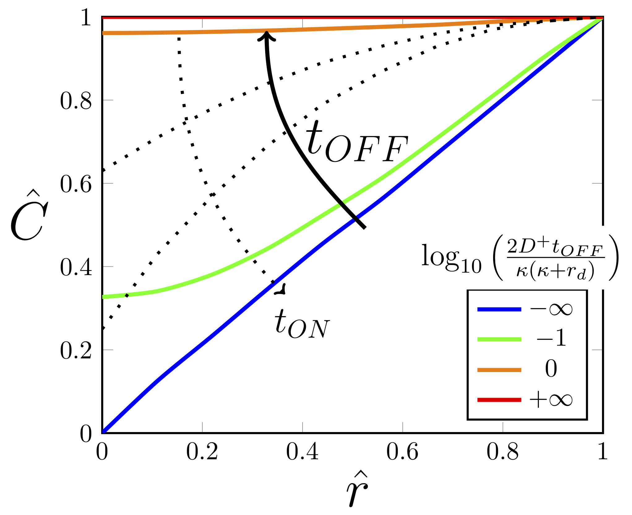
Figure 4: The concentration profile during the rest period $t_{OFF}$ (color) and the subsequent pulse interval $t_{ON}$ (dots).

The evolution of concentration profile $\hat{C}$ from Equation 22 during the entire cycle of pulse-rest has been shown in Figure 4 with the constants given in the Table 1.

Parameter	$D^{+}$	$\kappa$	$j$	$r_{d}$
Value	$2.58\times 10^{-10}$	$20$	$10^{-4}$	$20$
Unit	$m^{2}/s$	$\mu m$	$C/m^{2}s$	$nm$
Ref.	[16]	[30]	[47]	[47]

Table 1: Simulation Parameters.

3 Experimental

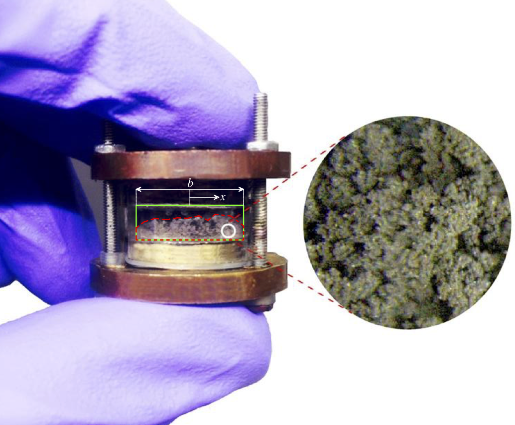
(a) Naked-eye observation of dendrites.[19]

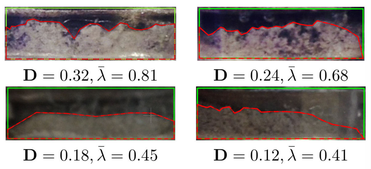
(b) Sample tracking of the suppression for $f=100Hz$.

(c) Extracting the dendrite measure from experimental images.

Figure 5: Experimental Procedure.

The dendritic measurements has been carried out in a manually-fabricated electrolytic cell[48], that provides the possibility of in-situ observation of growing dendrites from the periphery in real-time as shown in Figure 5a. The sandwich cell consists of two $Li^{0}$ foil disc electrodes ($D=1.59cm$) with the inter-electrode separation of $L=0.32cm$ by means of a transparent acrylic PMMA housing. The fabricated cells were filled with $0.4cm^{3}$ of LiPF₆ in a the stoichiometric compound of EC:EMC$\equiv$1:1. We performed the operations in an argon-filled glovebox($H_{2}O,O_{2}<0.5ppm$) . Multiple such cells were electrolyzed with current density pulse trains consisting of a range of frequencies $f$, generated by a programmable multichannel charger. After the passage of $48mAh$ ($\approx 173C$) through the cells, 3 images within the periphery of $120^{0}$ were taken by means of Leica M205FA optical microscope through the acrylic separator. The image processing algorithm given in the Figure 5c is described as below:

1. The RGB image is read to the program by 3 values of $\{R,G,B\}\in[0,255]$ and has been converted to a grayscale image $I$ with individual values of range $I_{i,j}\in[0,1]$.

2. The image is binarized from Otsu’s method. For this purpose a critical grayness threshold $I_{c}$ has been chosen to approximate the grayscale image $I$ with a binarized image $J$ as below:

$$J_{i,j}=\begin{cases}1&I_{i,j}\geq I_{c}\\ 0&I_{i,j}<I_{c}\end{cases}$$

the threshold value $I_{c}$ has been chosen to minimize the weighted intra-class variance $\sigma^{2}$ defined as:

$$\begin{cases}\sigma^{2}=\omega_{0}\sigma_{0}^{2}+\omega_{1}\sigma_{1}^{2}\\ \omega_{0}+\omega_{1}=1\end{cases}$$

where $\omega_{0}$ and $\omega_{1}$ are the total fraction of element divided by the value of $I_{c}$ and $\sigma_{0}^{2}$ and $\sigma_{1}^{2}$ are their respective variances.[49].

3. The circular sandwich cell with the radius $R$ has been divided of 3 arcs with the angle of ${\displaystyle\frac{2\pi}{3}}$ and width incremental length of $\delta x$, which is supposed to be projected to a 2D plane with the incremental width of $\delta x^{\prime}$. From Figure 5a due to geometry we have: $x={\displaystyle\frac{D}{2}}sin(\theta)$, $\rightarrow$ $dx={\displaystyle\frac{D}{2}}cos(\theta)d\theta$, where $cos(\theta)=\sqrt{{\displaystyle 1-\frac{4x^{2}}{D^{2}}}}$ ; hence:

$$\delta x^{\prime}=\frac{\delta x}{\sqrt{1-{\displaystyle\frac{4x^{2}}{D^{2}}}}}$$

where $D$ is diameter of the cell. [50]

4. Starting from the electrode surface, the occupied space by the dendrites has been calculated by the square site percolation paradigm. [51]

5. The infinitesimal calculations have been integrated and normalized to inter-electrode distance (${\displaystyle\hat{\lambda}_{i}:=\lambda_{i}/l}$ ) to get the dendrite measure $\bar{\lambda}$, as shown in Figure 5c as:

$$\bar{\lambda} =\frac{1}{\pi Dl}\sum_{k=1}^{3}\int_{-\frac{\pi}{3}}^{+\frac{\pi}{3}}\hat{\lambda}_{k}(\theta){\displaystyle\frac{D}{2}}d\theta$$ (34)

$$=\frac{1}{\pi Dl}\sum_{k=1}^{3}\int_{-\frac{\pi}{3}}^{+\frac{\pi}{3}}\frac{\hat{\lambda}_{k}(x)dx}{\sqrt{1-{\displaystyle\frac{4x^{2}}{D^{2}}}}}$$

The integral Equation 34 has been obtained by incremental sum from experimental data. The optimal duty cycle $\mathbf{D}$ has been considered where the sensitivity of dendrites metric $\bar{\lambda}$ to duty cycle $\mathbf{D}$ is less than $10\%$. Hence:

$$\mathbf{D_{opt}}:\equiv\left\{\frac{\Delta\bar{\lambda}}{\Delta\mathbf{D}}\leq 0.1\right\}$$

Figure 5b shows such investigation for the sample pulse frequency of $f=100Hz$. The experimental parameters for further data are given in the Table 2.

Parameter	$f$	$i$	$l$	$R$	$T$	$C_{\infty}$	$|\mathbf{\vec{E}}|_{max}$
Value	$\{25,40,100,250,1000\}$	$1$	$3.175$	$0.795$	$298$	$1$	$10^{8}$
Unit	$mHz$	$mA/cm^{2}$	$mm$	$cm$	$K$	$M$	$N/m$

Table 2: Experimental Parameters.

4 Results and discussion

4.1 Duty Cycle

Figure 6 visualizes the range of acceptable duty cycle $\mathbf{D}$ for the suppression of microstructures. In fact its theoretical limit can be obtained when the pulse frequency $f$ is increased indefinitely as:

$$\mathbf{D}_{max}=\lim_{f\to\infty}\frac{1}{\left(1+{\displaystyle\frac{|\vec{\textbf{E}}|}{RT}}\sqrt{{\displaystyle\frac{D^{+}}{2f}}}\right)^{2}+1}=\frac{1}{2}$$

Additionally in the Figure 6, the Controlled region shows the safe zone for pulse charging where the ionic progress in the idle period is competitive enough with the pulse duration. Vice versa, the Runaway region represents the regime where the average ionic lead during pulse wave takes over the rest period, and therefore the dendritic growth would be exacerbated. Nonetheless, the Intermediate region shows the role of random walk where the certainty is less than the other areas. The experimental observations in this Figure also illustrate a very high agreement with the analytical trend.

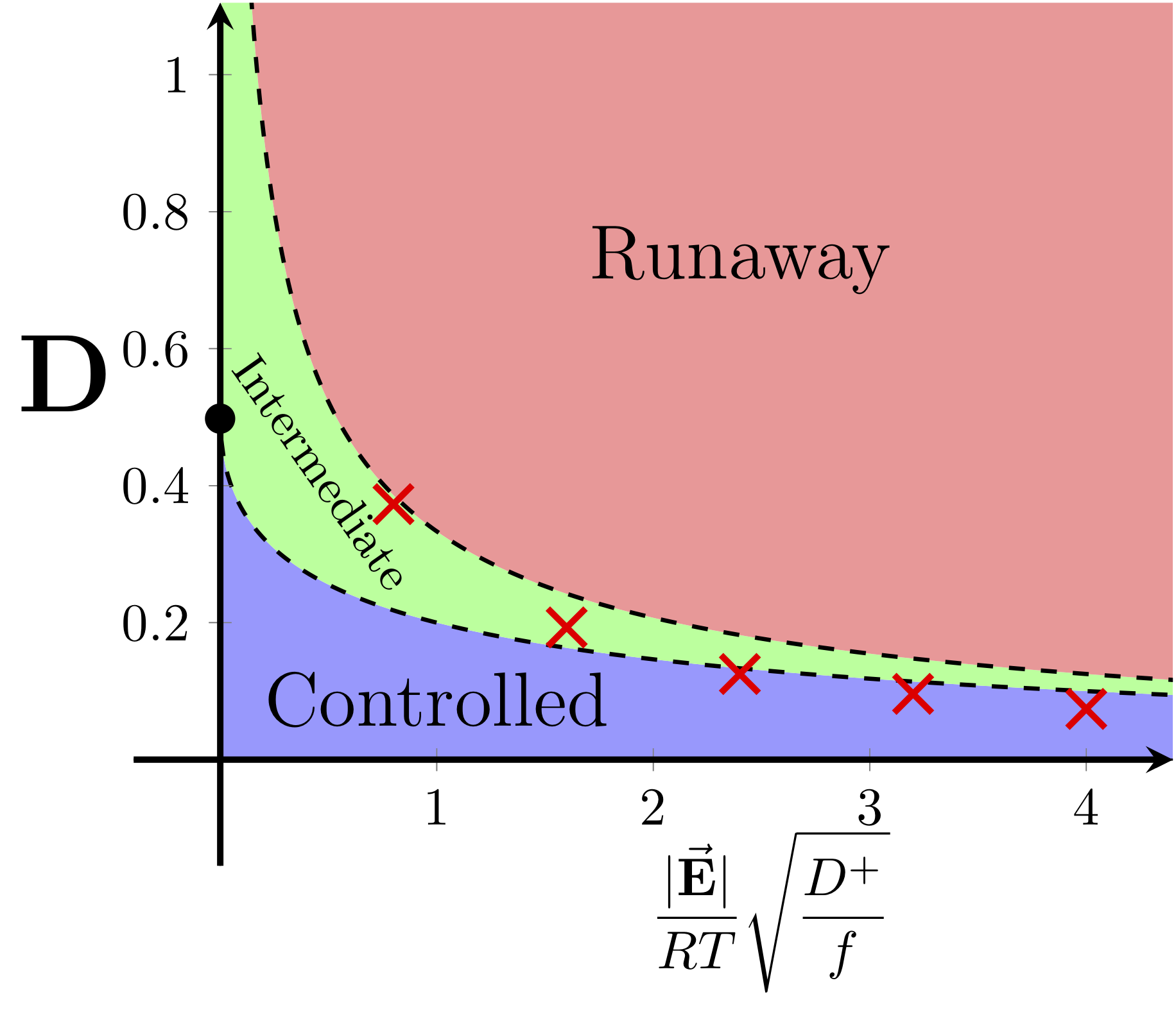
Figure 6: The regimes based on duty cycle $\mathbf{D}$ and frequency $f$ showing the safe/unsafe charging zones. $\times$: Experimental data , $\bullet$: Theoretical limit.

Additionally, it is obvious that the pulse duty cycle $\mathbf{D}$ correlates inversely with the diffusion coefficient $D^{+}$ and to a higher extend to the magnitude of the electric field $|\vec{\textbf{E}}|$. Both parameters exacerbate the growth kinetics and in trade-off, the duty cycle would have to become more conservative. In fact, the augmentation of electric field in the dendritic tips during the real-time growth causes the quickening growth behavior, which has been addressed before. [43, 31]

4.2 Concentration profile

Looking closer to the depletion-accrual cycle of concentration during full pulse-rest period shown in Figure 4, we have the following inequality:

$$\int_{0}^{1}\hat{C}(\hat{r},t)d\hat{r}\leq 1$$ (35)

The comparison of the dynamics of ionic concentration, versus the dendrite growth rate indicates that the electrodeposition occurs in a significantly faster kinetics than dendrites growth:

$$\frac{\partial\hat{C}}{\partial t}\gg\frac{\partial\hat{\lambda}}{\partial t}$$

Since the dendrites are the boundary condition for the concentration development per see, such a distinction implies that the concentration profile would occur in the quasi-steady state regime in the double layer region. This is particularly true during stage of instigation of microstructures, where the nucleation rate is negligible. Therefore the concentration profile would be obtained by solving the RHS of Equation 22 as:

$$\frac{\partial^{2}\hat{C}}{\partial\hat{r}^{2}}+\frac{\kappa}{r_{d}+\kappa\hat{r}}\frac{\partial\hat{C}}{\partial\hat{r}}\approx 0$$ (36)

Setting the boundary condition from Equation 24 as ${\displaystyle\frac{\partial\hat{C}}{\partial\hat{r}}(0,t)=-\frac{\kappa j}{C_{\infty}D^{+}}}$, one gets:

$$\frac{d\hat{C}}{d\hat{r}}\approx\frac{-\kappa r_{d}j}{C_{\infty}D^{+}(r_{d}+\kappa\hat{r})}$$

Integrating again and having ${\displaystyle\hat{C}(1,t)=1}$ leads to:

$$\hat{C}(\hat{r},t)\approx 1-\frac{r_{d}j}{C_{\infty}D^{+}}\ln\left(\frac{r_{d}+\kappa}{r_{d}+\kappa\hat{r}}\right)$$ (37)

For linearization the Equation 37 can be re-arranged as:

$$\hat{C}(\hat{r},t)\approx 1+\frac{r_{d}j}{C_{\infty}D^{+}}\ln\left(1-\frac{\kappa-\kappa\hat{r}}{r_{d}+\kappa}\right)$$

For the mesoscale dendrite the thickness of the double layer $\kappa$ is negligible relative to the radius of the dendrite $r_{d}$. (i.e. $\kappa\ll r_{d}$). therefore ${\displaystyle\frac{\kappa-\kappa\hat{r}}{r_{d}+\kappa}\to 0}$ and log term can be approximated with the first term of Taylor expansion as:

$$\hat{C}(\hat{r},t) \approx 1-\frac{r_{d}j}{C_{\infty}D^{+}}\frac{\kappa(1-\hat{r})}{r_{d}+\kappa}$$ (38)

$$\approx 1-\frac{\kappa j}{C_{\infty}D^{+}}(1-\hat{r})$$

Such a linear concentration profile has been addressed in the past for the flat electrodes as well. [31] This profile has been illustrated in Figure 4 as well. It is obvious that at the reaction sites ($\hat{r}\rightarrow 0$) the concentration correlates inversely with the ionic flux $j$. In order to have complete depletion in the reduction sites, we should have the following:

$$j_{*}=D^{+}\frac{C_{\infty}}{\kappa}$$

which resembles the flux from the linear concentration distribution throughout the entire span of double layer and has been expressed as the critical current density, where the electrode concentration goes to zero. [52, 53]

4.3 Relaxation time

The Equation 33 in fact resembles the Van Neumann stability criterion for the typical diffusion equation as: [54]

$$\frac{D^{+}\delta t}{\delta r^{2}}\leq\frac{1}{2}$$ (39)

the implication is shown in Equation 32 suggests that the relaxation time correlates with the geometric mean of the thickness of the double layer $\kappa$ and the outer radius $r_{O}=\kappa+r_{d}$. The relaxation profile during this time also has been shown in the Figure 4 where the marginal deviation from the absolutely uniform concentration distribution (i.e. where $t_{OFF}\to\infty$) could be due to the round off error as well as truncation error during the discrete computation.[55] The geometric mean correlation for the relaxation time has been addressed before as the RC time of the system for blocking flat electrodes [42] which implies that the regime of relaxation time would vary across the morphology of the electrodeposits with varying radius of curvature from atomic scale in the dendritic tips, to the completely flat surface in smooth areas ($r_{d}\in[r_{atom},\infty]$). Therefore the homogenized relaxation time would have the following span:

$$\frac{\kappa(\kappa+r_{d})}{D^{+}}\leq t_{OFF}^{opt}\leq\frac{\kappa l}{D^{+}}$$ (40)

Nevertheless, the overall relaxation time of the heterogeneous morphology is determined by the longest relaxation time as the most conservative case, belonging to the flat zones.

4.4 Geometry

As shown in Figure 3, the convex boundary of dendritic interface is exposed to expanded space in the double layer medium ($r_{O}>r_{d}$). Such geometry alters the dynamics of concentration gradient relative to flat surface during the pulse-rest cycle. During the pulse period (i.e. formation of concentration gradient) the dendritic sites have limited space for the higher feed of ions from the larges space. Hence, the depletion of concentration occurs in slower rate, whereas during the relaxation, there will be larger free domain to diffuse into, relative to flat surface. Therefore the relaxation occurs with faster rate for convex surfaces. This is also obvious from Equation 22 where the term ${\displaystyle\frac{1}{r}\frac{\partial}{\partial r}}$ would alter the concentration dynamics as illustrated in the Table 3. The sign of second derivate ${\displaystyle\frac{\partial^{2}C}{\partial r^{2}}}$ is easily discernible from curvature of the concentration profile in Figure 4, which is the identical for all morphologies concerned. [56, 57]. For convex dendrites, the curvature term slows down the formation of concentration gradient, whereas it accelerates the relaxation rate. Following the same phenomenology, the relaxation in concave surfaces (i.e. pores) occurs at faster dynamics , as the concentrated atoms have relatively less space to diffuse into. Respectively the curvature would resist the relaxation for the pores due to lack of space. Such dynamics translates into the number of iterations for convergence in our computations.

	Curvature	Convex (dendrites)		Concave (pores)
Period	${\displaystyle\frac{\partial^{2}C}{\partial r^{2}}}$	${\displaystyle\frac{1}{r}\frac{\partial C}{\partial r}}$	${\displaystyle\frac{\partial C}{\partial t}}$	${\displaystyle\frac{1}{r}\frac{\partial C}{\partial r}}$	${\displaystyle\frac{\partial C}{\partial t}}$
Pulse (formation)	$-$	$+$	Slower	$-$	Faster
Rest (relaxation)	$+$	$+$	Faster	$-$	Slower

Table 3: The role of curvature on concentration dynamics versus flat surface.

The concentration gradient $\nabla C$ plays the major role for nonuniform localization of dendritic structures and has a nonlinear behavior in time. During pulse period, as $\nabla C$ decreases, the rate of relaxation decreases as well and vanishes when converging to equilibrium (i.e. uniform profile). We define the depletion measure $\Delta(t)$ for tracking its dynamics as:

$$\Delta(t):=1-\hat{C}_{i}(t)$$ (41)

where $\hat{C}_{i}(t)$ is the concentration of the interface (i.e. surface of the dendrite). The variation of depletion measure $\Delta(t)$ during the full pulse-rest period is shown in Figure 8, assuming that the depletion current density meets the critical value (i.e. $j\geq j_{*}$).[52] As is discussed in Table 3, the formation of such gradient occurs in a longer time period than the Sand’s time [58], whereas the relaxation occurs faster rate (i.e. shorter time) than the flat electrode. This is also obvious from Equation 40.

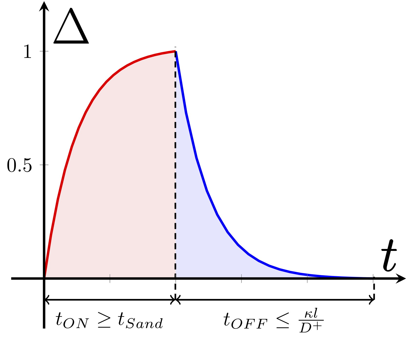
Figure 7: The time regime for concentration gradient in the convex dendrites.

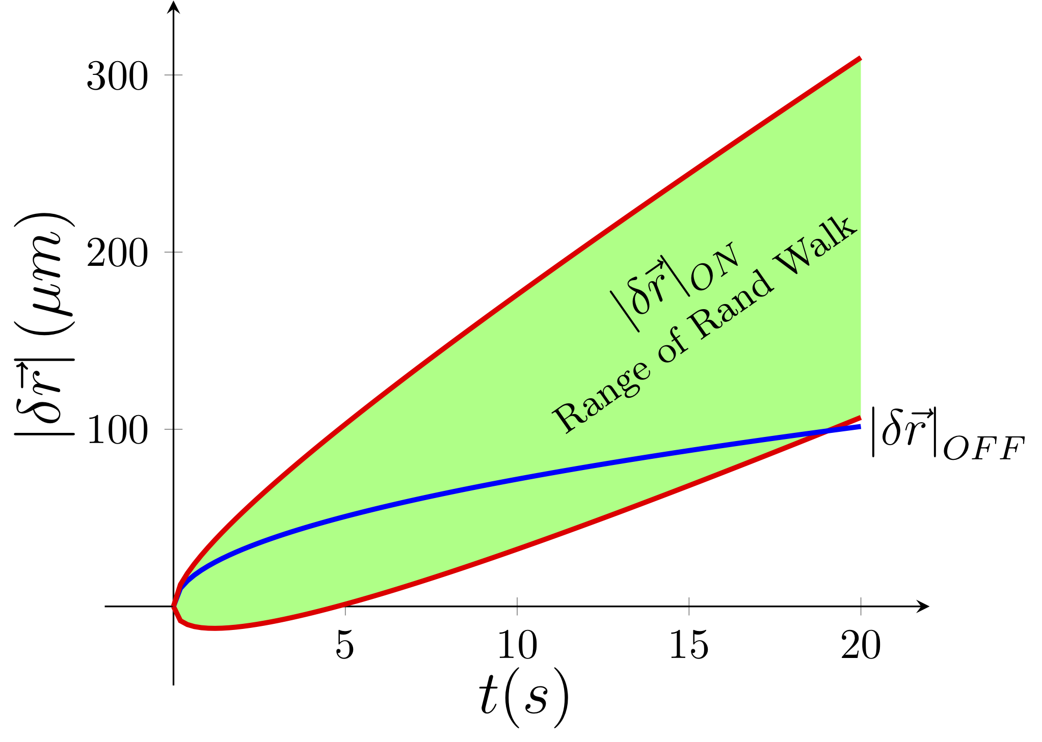
Figure 8: Extended range of random walk during pulse interval, compared with the progress of diffusion wave in the rest period.

Looking at the extended range of diffusion-migration dynamics at provided more insight to the range of duty cycle. The diffusion length scales with square root of time ($\delta\vec{r}_{D}\propto t^{\nicefrac{{1}}{{2}}}$) whereas the migration lead scales linearly with it ($\delta\vec{r}_{M}\propto t$). Therefore, one expects that given a sufficient time $\delta t_{eq}$ , the migration front would take over the diffusion lead. The hypothetical comparison of the progress of sole-diffusive and sole-migrative waves is possible from Equations 3 and 4 combined with the Einstein relationship ($D^{+}=\mu^{+}RT$ )[34]:

$$\delta t_{eq}=\frac{2RT}{\mu^{+}|\vec{\textbf{E}}|^{2}}$$ (42)

where $R$ is gas constant and $T$ is temperature. Closer look at the dynamics of progress during pulse and rest periods from Equation 9 leads to the Figure 8. It is clear that during the initial moments, the progress in the rest period could be more competitive with the pulse time. From the Equation 13, initially, the idle ratio $\gamma$ decays exponentially versus the dimension-less charge period $t_{ON}$. The exponential decay behavior indicates that relatively shorter amount of idle ratio is needed so that the diffusion lead would catch up the progress during applied pulse period. This is also obvious from Equation 12, as the term $\sqrt{\gamma}$ is comparable and in the order of $\gamma$. As the pulse period $t_{ON}$ increases, by neglecting the lower order terms, we reach to the limit $\gamma\propto t_{ON}$, which directly means $t_{OFF}\propto t_{ON}^{2}$ , therefore for higher applied pulse period $t_{ON}$, the equivalent idle period $t_{OFF}$ for concentration relaxation has to be significantly higher. As well in the Equation 15 if $t_{ON}$ increase indefinitely, the correlation of the needed rest period $t_{OFF}$ for the given pulse period $t_{ON}$ will move toward linear relationship from exponential decay behavior. On the other extreme, the application of indefinitely high pulse frequency $f$ (i.e. $t_{ON}\rightarrow 0$) might not let the ions reach the reaction sites. Therefore, the fine-enough pulse period would make the applied rest period for the charge relaxation easier to be competitive with it, as depicted in Figure 6.

List of Symbols

$f:$ pulse frequency ($Hz$)

$P$ : total period ($s$)

$t_{ON}:$ pulse period ($s$)

$t_{OFF}$: rest period ($s$)

$\delta t$: finite time increment ($s$)

$\hat{\textbf{g}}$ : normal vector in random direction ($[]$)

$\gamma$ : idle ratio ($[]$)

$\mathbf{D}$ : duty cycle ($[]$)

$C$: ionic concentration ($M$)

$\phi$ : electric field ($V$)

$\vec{\textbf{r}}_{D}$: diffusion vector ($m$)

$\vec{\textbf{r}}_{M}$: migration vector ($m$)

$t$ : time ($s$)

$D^{+}$: cationic diffusion coefficient ($m^{2}/s$)

$\vec{E}$ : electric field ($V/m$)

$R$ : gas constant (8.314$j/mol.K$)

$C_{i}$: concentration of the interface ($M$)

$\mu^{+}$: cationic ionic mobility ($m/V.s$)

$i$ : current density ($mA/cm^{2}$)

$j$ : current flux ($mol/(m^{2}s)$)

$D$ : diameter of the cell ($m$)

$F$ : Faraday’s constant ($96.5\text{ }\nicefrac{{kC}}{{mol}}$)

$z$: valence number ($[]$)

$\hat{\lambda}$: normalized dendrite measure ($[]$)

$\bar{\lambda}$ : Average normalized dendrite measure ($[]$)

$l$ : inter-electrode distance

$T$ : temperature ($K$)

$r$: radial distance ($m$)

$r_{d}$: radius of curvature of dendrite ($m$)

$r_{O}$: radius of curvature of the outer region ($m$)

$C_{\infty}$ : ambient concentration (i.e. electron-neutral) ($M$)

$\kappa$ : curvature of the interface ($m^{-1}$)

5 Conclusions

In this paper, we have performed analytical developments from stochastic ionic dynamics for the effective suppression of growing dendritic microstructures during electrodeposition. We defined such square pulse charging parameters in terms of the range of pulse duty cycle $\mathbf{D}$ and the respective idle time period $t_{OFF}$. Our model considers the localizations of both ionic concentration and electric field within the interface of the electrochemical cell, where the nonlinear role of the dendrite curvature on the relaxation is demonstrated in terms of cell geometry and the transport property of the electrolyte solution. The results are useful for estimating the effective charging for dendrite-prone electrochemical environments, particularly those of involving metallic electrodes (i.e. lithium, etc.).

References

- [1] Zhe Li, Jun Huang, Bor Yann Liaw, Viktor Metzler, and Jianbo Zhang. A review of lithium deposition in lithium-ion and lithium metal secondary batteries. J. Power Sources, 254:168–182, 2014.
- [2] Pucheng Pei, Keliang Wang, and Ze Ma. Technologies for extending zinc air batterys cyclelife: A review. Applied Energy, 128:315–324, 2014.
- [3] Michael D Slater, Donghan Kim, Eungje Lee, and Christopher S Johnson. Sodium-ion batteries. Adv. Funct. Mater., 23(8):947–958, 2013.
- [4] Siyuan Li, Jixiang Yang, and Yingying Lu. Lithium metal anode. Encyclopedia of Inorganic and Bioinorganic Chemistry, pages 1–21.
- [5] W. Xu, J. L. Wang, F. Ding, X. L. Chen, E. Nasybutin, Y. H. Zhang, and J. G. Zhang. Lithium metal anodes for rechargeable batteries. Energy and Environmental Science, 7(2):513–537, 2014.
- [6] Kang Xu. Nonaqueous liquid electrolytes for lithium-based rechargeable batteries. Chemical Reviews-Columbus, 104(10):4303–4418, 2004.
- [7] Yanguang Li and Hongjie Dai. Recent advances in zinc–air batteries. Chem. Soc. Rev., 43(15):5257–5275, 2014.
- [8] F. Orsini A.D. Pasquier B. Beaudoin J.M. Tarascon et al. In situ scanning electron microscopy (sem) observation of interfaces with plastic lithium batteries. J. Power Sources, 76:19–29, 1998.
- [9] C. Monroe and J. Newman. The effect of interfacial deformation on electrodeposition kinetics. J. Electrochem. Soc., 151(6):A880–A886, 2004.
- [10] Christoffer P Nielsen and Henrik Bruus. Morphological instability during steady electrodeposition at overlimiting currents. arXiv preprint arXiv:1505.07571, 2015.
- [11] PP Natsiavas, K Weinberg, D Rosato, and M Ortiz. Effect of prestress on the stability of electrode–electrolyte interfaces during charging in lithium batteries. Journal of the Mechanics and Physics of Solids, 95:92–111, 2016.
- [12] Katherine J Harry, Daniel T Hallinan, Dilworth Y Parkinson, Alastair A MacDowell, and Nitash P Balsara. Detection of subsurface structures underneath dendrites formed on cycled lithium metal electrodes. Nat. Mater., 13(1):69–73, 2014.
- [13] J. Steiger, D. Kramer, and R. Monig. Mechanisms of dendritic growth investigated by in situ light microscopy during electrodeposition and dissolution of lithium. J. Power Sources, 261:112–119, 2014.
- [14] N. Schweikert, A. Hofmann, M. Schulz, M. Scheuermann, S. T. Boles, T. Hanemann, H. Hahn, and S. Indris. Suppressed lithium dendrite growth in lithium batteries using ionic liquid electrolytes: Investigation by electrochemical impedance spectroscopy, scanning electron microscopy, and in situ li-7 nuclear magnetic resonance spectroscopy. J. Power Sources, 228:237–243, 2013.
- [15] Reza Younesi, Gabriel M Veith, Patrik Johansson, Kristina Edström, and Tejs Vegge. Lithium salts for advanced lithium batteries: Li-metal, li-o 2, and li-s. Energy and Environmental Science, 8(7):1905–1922, 2015.
- [16] C. Brissot, M. Rosso, J. N. Chazalviel, and S. Lascaud. In situ concentration cartography in the neighborhood of dendrites growing in lithium/polymer-electrolyte/lithium cells. J. Electrochem. Soc., 146(12):4393–4400, 1999.
- [17] I. W. Seong, C. H. Hong, B. K. Kim, and W. Y. Yoon. The effects of current density and amount of discharge on dendrite formation in the lithium powder anode electrode. J. Power Sources, 178(2):769–773, 2008.
- [18] GM Stone, SA Mullin, AA Teran, DT Hallinan, AM Minor, A Hexemer, and NP Balsara. Resolution of the modulus versus adhesion dilemma in solid polymer electrolytes for rechargeable lithium metal batteries. J. Electrochem. Soc., 159(3):A222–A227, 2012.
- [19] Asghar Aryanfar, Tao Cheng, Agustin J Colussi, Boris V Merinov, William A Goddard III, and Michael R Hoffmann. Annealing kinetics of electrodeposited lithium dendrites. The Journal of chemical physics, 143(13):134701, 2015.
- [20] Yuanzhou Yao, Xiaohui Zhao, Amir A Razzaq, Yuting Gu, Xietao Yuan, Rahim Shah, Yuebin Lian, Jinxuan Lei, Qiaoqiao Mu, Yong Ma, et al. Mosaic rgo layer on lithium metal anodes for effective mediation of lithium plating and stripping. Journal of Materials Chemistry A, 2019.
- [21] Ji Qian, Yu Li, Menglu Zhang, Rui Luo, Fujie Wang, Yusheng Ye, Yi Xing, Wanlong Li, Wenjie Qu, Lili Wang, et al. Protecting lithium/sodium metal anode with metal-organic framework based compact and robust shield. Nano Energy, 2019.
- [22] Wei Deng, Wenhua Zhu, Xufeng Zhou, Fei Zhao, and Zhaoping Liu. Regulating capillary pressure to achieve ultralow areal mass loading metallic lithium anodes. Energy Storage Materials, 2019.
- [23] Alexander W Abboud, Eric J Dufek, and Boryann Liaw. Implications of local current density variations on lithium plating affected by cathode particle size. Journal of The Electrochemical Society, 166(4):A667–A669, 2019.
- [24] Chen Xu, Zeeshan Ahmad, Asghar Aryanfar, Venkatasubramanian Viswanathan, and Julia R Greer. Enhanced strength and temperature dependence of mechanical properties of li at small scales and its implications for li metal anodes. Proceedings of the National Academy of Sciences, 114(1):57–61, 2017.
- [25] Peng Wang, Wenjie Qu, Wei-Li Song, Haosen Chen, Renjie Chen, and Daining Fang. Electro–chemo–mechanical issues at the interfaces in solid-state lithium metal batteries. Advanced Functional Materials, page 1900950, 2019.
- [26] R. Bhattacharyya, B. Key, H. L. Chen, A. S. Best, A. F. Hollenkamp, and C. P. Grey. In situ nmr observation of the formation of metallic lithium microstructures in lithium batteries. Nat. Mater., 9(6):504–510, 2010.
- [27] S Chandrashekar, Nicole M Trease, Hee Jung Chang, Lin-Shu Du, Clare P Grey, and Alexej Jerschow. 7li mri of li batteries reveals location of microstructural lithium. Nat. Mater., 11(4):311–315, 2012.
- [28] Yunsong Li and Yue Qi. Energy landscape of the charge transfer reaction at the complex li/sei/electrolyte interface. Energy & Environmental Science, 2019.
- [29] Laleh Majari Kasmaee, Asghar Aryanfar, Zarui Chikneyan, Michael R Hoffmann, and AgustÃn J Colussi. Lithium batteries: Improving solid-electrolyte interphases via underpotential solvent electropolymerization. Chem. Phys. Lett., 661:65–69, 2016.
- [30] J. N. Chazalviel. Electrochemical aspects of the generation of ramified metallic electrodeposits. Phys. Rev. A, 42(12):7355–7367, 1990.
- [31] C. Monroe and J. Newman. Dendrite growth in lithium/polymer systems - a propagation model for liquid electrolytes under galvanostatic conditions. J. Electrochem. Soc., 150(10):A1377–A1384, 2003.
- [32] Thomas A Witten and Leonard M Sander. Diffusion-limited aggregation. Phys. Rev. B, 27(9):5686, 1983.
- [33] Rui Zhang, Xin Shen, Xin-Bing Cheng, and Qiang Zhang. The dendrite growth in 3d structured lithium metal anodes: Electron or ion transfer limitation? Energy Storage Materials, 2019.
- [34] Allen J. Bard and Larry R. Faulkner. Electrochemical methods: fundamentals and applications. 2 New York: Wiley, 1980., 1980.
- [35] Deepti Tewari and Partha P Mukherjee. Mechanistic understanding of electrochemical plating and stripping of metal electrodes. Journal of Materials Chemistry A, 7(9):4668–4688, 2019.
- [36] Martin Z Bazant, Brian D Storey, and Alexei A Kornyshev. Double layer in ionic liquids: Overscreening versus crowding. Phys. Rev. Lett., 106(4):046102, 2011.
- [37] V. Fleury. Branched fractal patterns in non-equilibrium electrochemical deposition from oscillatory nucleation and growth. Nature, 390(6656):145–148, 1997.
- [38] Asghar Aryanfar, Daniel J Brooks, AgustÃn J Colussi, Boris V Merinov, William A Goddard III, and Michael R Hoffmann. Thermal relaxation of lithium dendrites. Phys. Chem. Chem. Phys., 17(12):8000–8005, 2015.
- [39] Jun Li, Edward Murphy, Jack Winnick, and Paul A Kohl. The effects of pulse charging on cycling characteristics of commercial lithium-ion batteries. J. Power Sources, 102(1):302–309, 2001.
- [40] M. S. Chandrasekar and M. Pushpavanam. Pulse and pulse reverse plating - conceptual, advantages and applications. Electrochim. Acta, 53(8):3313–3322, 2008.
- [41] Asghar Aryanfar, Daniel Brooks, Boris V. Merinov, William A. Goddard Iii, AgustÃn J. Colussi, and Michael R. Hoffmann. Dynamics of lithium dendrite growth and inhibition: Pulse charging experiments and monte carlo calculations. The Journal of Physical Chemistry Letters, 5(10):1721–1726, 2014.
- [42] M. Z. Bazant, K. Thornton, and A. Ajdari. Diffuse-charge dynamics in electrochemical systems. Physical Review E, 70(2), 2004.
- [43] Asghar Aryanfar, Daniel J Brooks, and William A Goddard. Theoretical pulse charge for the optimal inhibition of growing dendrites. MRS Advances, 3(22):1201–1207, 2018.
- [44] Jean Philibert. One and a half century of diffusion: Fick, einstein, before and beyond. Diffusion Fundamentals, 4(6):1–19, 2006.
- [45] Philip J Pritchard, John W Mitchell, and John C Leylegian. Fox and McDonald’s Introduction to Fluid Mechanics, Binder Ready Version. John Wiley & Sons, 2016.
- [46] Mohamed A Khamsi and William A Kirk. An introduction to metric spaces and fixed point theory, volume 53. John Wiley & Sons, 2011.
- [47] J. L. Barton and J. O’M Bockris. The electrolytic growth of dendrites from ionic solutions. Proceedings of the Royal Society of London. Series A, Mathematical and Physical Sciences, 268(1335):485–505, 1962.
- [48] Asghar Aryanfar. Method and device for dendrite research and discovery in batteries, April 11 2017. US Patent 9,620,808.
- [49] Nobuyuki Otsu. A threshold selection method from gray-level histograms. Automatica, 11(285-296):23–27, 1975.
- [50] Asghar Aryanfar, Daniel J Brooks, Agustin J Colussi, and Michael R Hoffmann. Quantifying the dependence of dead lithium losses on the cycling period in lithium metal batteries. Phys. Chem. Chem. Phys., 16(45):24965–24970, 2014.
- [51] Asghar Aryanfar, William Goddard III, and Jaime Marian. Constriction percolation model for coupled diffusion-reaction corrosion of zirconium in pwr. Corrosion Science, 2019.
- [52] C. Brissot, M. Rosso, J. N. Chazalviel, and S. Lascaud. Dendritic growth mechanisms in lithium/polymer cells. J. Power Sources, 81:925–929, 1999.
- [53] Yuqing Chen, Yang Luo, Hongzhang Zhang, Chao Qu, Huamin Zhang, and Xianfeng Li. The challenge of lithium metal anodes for practical applications. Small Methods, page 1800551, 2019.
- [54] Eugene Isaacson and Herbert Bishop Keller. Analysis of numerical methods. Courier Corporation, 2012.
- [55] William Edmund Milne and WE Milne. Numerical solution of differential equations, volume 19. Wiley New York, 1953.
- [56] C. Leger, J. Elezgaray, and F. Argoul. Dynamical characterization of one-dimensional stationary growth regimes in diffusion-limited electrodeposition processes. Physical Review E, 58(6):7700–7709, 1998.
- [57] C. Leger, J. Elezgaray, and F. Argoul. Experimental demonstration of diffusion-limited dynamics in electrodeposition. Phys. Rev. Lett., 78(26):5010–5013, 1997.
- [58] M. Rosso. Electrodeposition from a binary electrolyte: new developments and applications. Electrochim. Acta, 53(1):250–256, 2007.