LRG-BEASTS: Transmission Spectroscopy and Retrieval Analysis of the Highly-Inflated Saturn-mass Planet WASP-39b

Abstract

We present a ground-based transmission spectrum and comprehensive retrieval analysis of the highly inflated Saturn-mass planet WASP-39b. We obtained low-resolution spectra ($R\approx 400$) of a transit of WASP-39b using the ACAM instrument on the 4.2 m William Herschel Telescope as part of the LRG-BEASTS survey. Our transmission spectrum is in good agreement with previous ground- and space-based observations of WASP-39b, and covers a wavelength range of 4000–9000 Å. Previous analyses of this exoplanet have retrieved water abundances that span more than four orders of magnitude, which in turn lead to conclusions of a subsolar or highly supersolar atmospheric metallicity. In order to determine the cause of the large discrepancies in the literature regarding WASP-39b’s atmospheric metallicity, we performed retrieval analyses of all literature data sets. Our retrievals, which assume equilibrium chemistry, recovered highly supersolar metallicities for all data sets. When running our retrievals on a combined spectrum, spanning 0.3–5 $\mu$m, we recovered an atmospheric metallicity of $282^{+65}_{-58}\times$ solar. We find that stellar activity has a negligible effect on the derived abundances and instead conclude that different assumptions made during retrieval analyses lead to the reported water abundances that differ by orders of magnitude. This in turn has significant consequences for the conclusions we draw. This is the fourth planet to be observed as part of the LRG-BEASTS survey, which is demonstrating that 4 m class telescopes can obtain low-resolution transmission spectra with precisions of around one atmospheric scale height.

1 Introduction

In the 17 years since the first detection of an exoplanet atmosphere (Charbonneau et al., 2002), the atmospheres of dozens of exoplanets have been characterized in transmission. These observations have revealed a remarkable diversity across the exoplanet population, from (relatively) small exoplanets with cloudy atmospheres (e.g., Kreidberg et al., 2014) to large exoplanets with clear atmospheres (e.g., Nikolov et al., 2018). A recent survey of 10 hot Jupiters highlighted this diversity by revealing a continuum from clear to cloudy atmospheres (Sing et al., 2016).

Clouds and hazes are problematic for atmospheric studies as they mute, or sometimes entirely mask, absorption lines of interest (e.g., Pont et al., 2008; Mallonn et al., 2016; Kirk et al., 2017; Louden et al., 2017). In particular, they can mask features originating at altitudes lower than the aerosols themselves, such as the pressure-broadened wings of Na and K. Indeed, the pressure-broadened wings have only been observed in two exoplanets to date (WASP-39b, Fischer et al. 2016; Sing et al. 2016; and WASP-96b, Nikolov et al. 2018), serving to highlight the near-ubiquitous nature of clouds and hazes.

Given the impact aerosols have on atmospheric characterization, it would be useful to know a priori whether a planet is likely to be clear or cloudy. For this reason, there have been a number of recent studies looking for correlations between planetary parameters and the presence of clouds and hazes (Heng, 2016; Sing et al., 2016; Stevenson, 2016; Crossfield & Kreidberg, 2017; Fu et al., 2017). While these studies have been conducted over relatively small sample sizes, there is growing evidence that hotter planets are more likely than cooler planets to be cloud free (e.g., WASP-121b, Evans et al., 2018; KELT-9b, Hoeijmakers et al., 2018, 2019). This might be due, in part, to their temperatures being too high for many species to condense. Also, at hotter temperatures, the main carbon-bearing species is CO and not CH₄, the photodissociation of which is responsible for soot-like hazes (e.g., Morley et al., 2015). However, theory predicts that clouds (Wakeford & Sing, 2015; Wakeford et al., 2017) and sulfur hazes (Zahnle et al., 2009) can exist even in the hottest exoplanets.

In addition to the effects of clouds and hazes described above, they can also lead to steeper slopes than expected from H₂ scattering (e.g., Pont et al., 2013). The gradient of the slope can be used to infer information about the condensates responsible (e.g., Wakeford & Sing, 2015; Pinhas & Madhusudhan, 2017) and be used to determine the mean molecular weight of the atmosphere (e.g., Benneke & Seager, 2012). The mean molecular weight obtained from the optical slope can then be used to break a degeneracy between the volume mixing ratios of gases derived from infrared data and the scale height of the atmosphere.

Optical data are also useful to provide a reference pressure, which can lead to significant improvements in the precisions of abundances derived from infrared data (e.g., Griffith, 2014; Wakeford et al., 2018; Pinhas et al., 2019) and is necessary for a unique constraint on the mixing ratios of absorbers and inactive gases (Benneke & Seager, 2012). Indeed, in a retrieval study of 10 hot Jupiters, Pinhas et al. (2019) found that optical data were essential to obtain a reliable constraint on the abundances derived from infrared data. For the case of HD 209458b, they found that the combination of optical data with infrared data led to a $3\times$ better constraint on the abundance of water than infrared data alone, as the optical data were able to lift the degeneracy between reference pressure and abundance (e.g., Lecavelier Des Etangs et al., 2008; Griffith, 2014; Heng & Kitzmann, 2017), as the absolute number densities of species cannot be calculated without an absolute pressure scale (Benneke & Seager, 2012). Not only does the inclusion of optical data improve the constraint on water abundance, but it can actually lead to a different measured abundance of water (see Figure 7 of Pinhas et al., 2019).

The study of clouds and hazes and the importance of optical data on precise atmospheric characterization necessitates further observations of planets at optical wavelengths. This is the principal motivation behind the Low-Resolution Ground-Based Exoplanet Atmosphere Survey using Transmission Spectroscopy (LRG-BEASTS; ‘large beasts’) project. LRG-BEASTS is pioneering the use of 4 m class telescopes for low-resolution transmission spectroscopy and has demonstrated that such facilities can obtain transmission spectra with precisions of 1 atmospheric scale height (Kirk et al., 2017, 2018; Louden et al., 2017). Such studies are often limited by systematic and not photon noise, and so larger apertures do not necessarily provide greater precision. To date, LRG-BEASTS has revealed a Rayleigh scattering haze in the atmosphere of HAT-P-18b (Kirk et al., 2017), a gray cloud deck in the atmosphere of WASP-52b (Kirk et al., 2016; Louden et al., 2017), and a haze in the atmosphere of WASP-80b (Kirk et al., 2018). All of these planets are relatively cool ($T\mathrm{{}_{eq}}<1315$ K) and our detection of clouds and hazes is in agreement with the tentative correlation between the presence of aerosols and equilibrium temperature.

Other recent transmission spectroscopy highlights include the first detection of He in an exoplanet atmosphere (that of the evaporating planet WASP-107b; Spake et al., 2018), and high-resolution observations revealing metals such as atomic Fe and Ti in the atmosphere of an ultrahot Jupiter (KELT-9b; Hoeijmakers et al. 2018, 2019). While transit observations give information about the limb of an exoplanet’s atmosphere at pressures of millibars to microbars, observations during the secondary eclipse provide information at pressures of bars to millibars and can provide information about atmospheric species complementary to information gathered during transit. Recent highlights of secondary eclipse observations include a well-constrained metallicity measurement of the hot Jupiter WASP-18b, allowing for comparison with metallicity measurements made via transmission spectroscopy (Arcangeli et al., 2018). Finally, phase curve observations can provide information about atmospheric circulation and heat transport. Recently, HAT-P-7b was observed to show a shift in the location of its hottest point, indicating changing weather patterns within the planet’s atmosphere (Armstrong et al., 2016).

1.1 WASP-39b

WASP-39b (Faedi et al., 2011) is a highly inflated Saturn-mass planet, with a mass of 0.28 $M_{\mathrm{J}}$ and a radius of 1.2 $R_{\mathrm{J}}$. It orbits its G8 host with a period of 4.05 days and has an equilibrium temperature of 1116 K (Faedi et al., 2011). This temperature puts it at the boundary at which CO takes over from CH₄ as the main carbon-bearing species, which occurs at $\sim$1100 K, potentially removing CH₄-derived aerosols from its atmosphere (Morley et al., 2015). When considering the aerosol–temperature correlations mentioned above, it is difficult to predict a priori whether its atmosphere is more likely to be clear or cloudy. Regardless of this, WASP-39b is an excellent target for transmission spectroscopy owing to its large atmospheric scale height (983 km) and transit depth per scale height of $452$ ppm. For this reason, there have been previous studies of WASP-39b’s transmission spectrum.

Hubble Space Telescope (HST)/STIS observations of WASP-39b detected Rayleigh scattering in addition to the pressure-broadened wings of both sodium and potassium (Fischer et al., 2016; Sing et al., 2016). This transmission spectrum could be described by either a clear, H₂-dominated atmosphere at solar or subsolar metallicities, or a solar metallicity atmosphere with a weak haze layer (Fischer et al., 2016). This was the first time that the pressure-broadened wings of both alkali lines had been detected in an exoplanet atmosphere, as these had previously always been masked by aerosols at low pressures.

In a retrieval analysis of the HST/STIS and Spitzer data presented in Sing et al. (2016), Barstow et al. (2017) found that gray atmosphere models provided the best fit to WASP-39b’s transmission spectrum, although clear-atmosphere and Rayleigh scattering solutions also existed.

Nikolov et al. (2016) observed WASP-39b using Very Large Telescope (VLT)/FORS in order to provide a ground-based transmission spectrum both to complement, and compare with, the HST results of Fischer et al. (2016) and Sing et al. (2016). The VLT transmission spectrum was in good agreement with that of HST, finding sodium and potassium features extending over $\sim$5 and 3 atmospheric scale heights, respectively. However, while the Na detection was statistically significant, the detection of K had a significance of only 1.2$\sigma$. The VLT study found that the atmosphere was most consistent with a cloud-free solar metallicity atmosphere with either uniform absorption from large particles or $10\times$ Rayleigh scattering from small particles. They were, however, able to rule out strong Rayleigh scattering extending across the entire optical regime and also the presence of a cloud deck.

Recently, Wakeford et al. (2018) presented new HST/WFC3 measurements centered around the 1.4 $\mu$m water feature. Their precise observations and wide wavelength coverage, when combined with the HST/STIS and VLT observations discussed above (Fischer et al., 2016; Nikolov et al., 2016; Sing et al., 2016), allowed them to constrain the planet’s atmospheric metallicity to be 151${}^{+48}_{-46}\times$ solar, using water as a proxy for heavy-element abundance. When plotted against the mass-metallicity relation of the solar system, Wakeford et al. (2018) showed that this metallicity is higher than expected from this trend, although they noted that there is significant scatter expected (Thorngren et al., 2016). Its metallicity led Wakeford et al. (2018) to suggest that WASP-39b formed far out in the disk in a region rich with heavy-element planetesimals.

Furthermore, Wakeford et al. (2018) found that the inclusion of optical data, in addition to their WFC3 near-infrared data, resulted in much tighter constraints on the retrieved atmospheric abundances than when just using the WFC3 data alone. In particular, the inclusion of optical data led to a $\sim$2$\times$ improvement in the abundance constraint of water and 0.5 dex improvement in the precision of [M/H]. This was an excellent demonstration of the necessity of optical data to constrain the effects of clouds and hazes on infrared data, which will become increasingly important with the launch of James Webb Space Telescope (JWST).

Tsiaras et al. (2018) presented their own analysis of the same HST/WFC3 data set used in Wakeford et al. (2018). However, Tsiaras et al. (2018) only used data from the G141 grism, covering a wavelength range of 1.1–1.6 $\mu$m, while Wakeford et al. (2018) additionally used the G102 grism, extending their HST/WFC3 data down to 0.8 $\mu$m. When using the G141 data set alone, Tsiaras et al. (2018) calculated WASP-39b’s ($\log_{10}$) water abundance to be $-5.94\pm 0.61$, which is $\approx 10^{-3}\times$ solar and differed significantly with the metallicity found by Wakeford et al. (2018).

Pinhas et al. (2018) performed retrievals on the WFC3 data provided in Tsiaras et al. (2018) in addition to the HST/STIS and Spitzer data presented in Sing et al. (2016). This was the first retrieval performed on WASP-39b data that accounted for stellar activity, and Pinhas et al. (2018) found evidence for substantial heterogeneity on the host star. This is despite WASP-39 showing weak Ca II H and K emission (Faedi et al., 2011; Mancini et al., 2018), and no photometric modulation (Fischer et al., 2016). Using this retrieval code, Pinhas et al. (2019) found WASP-39b to have an H₂O abundance of $0.1^{+0.42}_{-0.08}\times$ solar, significantly different from the $151^{+48}_{-46}\times$ solar metallicity atmosphere found by Wakeford et al. (2018).

Fisher & Heng (2018) also performed a retrieval analysis on WASP-39b, using only the data set of Tsiaras et al. (2018). They found a ($\log_{10}$) water abundance of $-2.3^{+0.4}_{-0.67}$, three orders of magnitude greater than Tsiaras et al. (2018) despite an identical data set being used.

This wide range of derived metallicities and the potential impact of stellar activity necessitate further study of this planet.

The paper is organized as follows. In section 2 we present our WHT/ACAM observations. In sections 3 and 4 we present the reduction and fitting of our data. The results of this data analysis are presented in section 5 and the combined retrieval analysis is given in section 6. Our discussion and conclusions are presented in sections 7 and 8.

2 Observations

We observed a single transit of WASP-39b on the night of 2016 May 3 using the low-resolution ($R\approx 400$) spectrograph ACAM (Benn et al., 2008) on the 4.2 m William Herschel Telescope (WHT). This is the same instrument as used in our previous observations of HAT-P-18b (Kirk et al., 2017), WASP-52b (Louden et al., 2017) and WASP-80b (Kirk et al., 2018).

ACAM is well suited for transmission spectroscopy owing to its wide wavelength range ($\sim$3500–9200 Å), wide field of view (allowing for a greater choice of comparison stars), and wide slits (negating the potential for differential slit losses between the target and comparison). We chose to use ACAM to perform transmission spectroscopy owing to its simple optical design that uses a grism, which minimizes the potential for instrument-related systematics (such as was previously seen in VLT spectra, which was caused by its Linear Atmospheric Dispersion Corrector; Boffin et al., 2015).

A total of 176 biases were obtained and median-combined to form a master bias. Seventy-one spectroscopic sky flats were obtained at twilight through the same slit as used in the science frames. These were median-combined following the removal of a master bias to create a master flat. In order to remove the sky lines from the master flat, a running median was calculated for each column of the master flat using a sliding box of 5 pixels. This box width was found to remove the sky lines while retaining the pixel-to-pixel variations. Each column of the master flat was then divided by the running median along each column to remove the sky lines.

We obtained 179 spectra of WASP-39 and a comparison star simultaneously observed through a 40^′′ wide slit in order to remove telluric effects by performing differential photometry. The target and comparison are shown in Figure 1 (top panel). Our choice of comparison star was determined by the length of the slit (7.6^′) and the desire to get as close a match as possible in magnitude and color to WASP-39 in order to optimize the telluric correction. The comparison star chosen was 2MASS J14292245–0321010, at a distance of 5.73^′ from WASP-39 with $\Delta V=1.1$ and $\Delta(B-V)=0.25$ compared with WASP-39. Figure 2 shows diagnostic plots of the night’s data.

The observations were conducted from air mass 1.58 $\rightarrow$ 1.18 $\rightarrow$ 2.26. An exposure time of 120 s was used, other than frames 7, 8, and 9 where a 180 s exposure time was used. The readout time was 10 s. We applied a small defocus and made manual guiding corrections to the telescope when the $x$ and $y$ positions of the spectral traces were observed to drift by $\gtrsim 1$ pixel ($\approx 0.25^{\prime\prime}$; Figure 2). The moon was not visible throughout the duration of our observations.

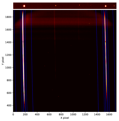
Figure 1: Top panel: image taken through the 40^′′ slit. WASP-39 is the left-hand bright star, and the comparison is the right-hand bright star. This panel is cropped vertically. Bottom panel: an example science frame. WASP-39 is the left-hand bright trace, and the comparison is the right-hand bright trace. The solid blue lines show the target aperture, and the dashed lines indicate the region over which the background was calculated.

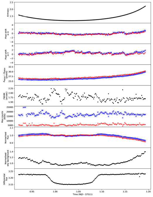
Figure 2: Diagnostic plots of the night’s data, all plotted with time on the $x$-axis. Top panel: variation of air mass across the observations. Second panel: the shift in the target’s spectrum (blue crosses) and comparison’s spectrum (red pluses) along the spatial direction. Third panel: the shift in the target’s spectrum (blue crosses) and comparison’s spectrum (red pluses) along the dispersion direction. Fourth panel: rotation of the target’s spectrum (blue crosses) and comparison’s spectrum (red pluses) as measured by the difference in the traces’ locations at red and blue wavelengths. Fifth panel: the variation in FWHM across the night. Sixth panel: the maximum counts recorded in the target’s spectrum (blue crosses) and comparison’s spectrum (red pluses). Seventh panel: the raw white-light curves of the target (blue crosses) and comparison (red pluses). Eighth panel: the normalized sky background. Bottom panel: WASP-39’s white-light curve following division by the comparison’s light curve.

3 Data reduction

To reduce the data, we used our own custom-built Python scripts as introduced in Kirk et al. (2017, 2018) and described in detail in Kirk (2018).

Following the bias and flat-field corrections using the master bias and master flat discussed in section 2, the spectral traces were extracted for the target and comparison for each of the 179 science frames. This was performed by fitting a Gaussian in the spatial direction to each trace at each row on the CCD. This gave the center of both traces as a function of $y$ (the dispersion direction). A fourth-order polynomial was then fitted to the centers calculated by the Gaussian fitting to give a smooth function of $y$.

Following the evaluation of the target’s and comparison’s traces as a function of $y$, aperture photometry was then performed for each row along the dispersion direction after removal of the sky background. To calculate the sky background, a quadratic polynomial was fitted between two regions on either side of the traces and interpolated across the traces (along the spatial direction). Any stars falling within the background regions were masked from the polynomial fit as were pixels that were greater than three standard deviations from the mean (such as due to cosmic rays). Additionally, at $y$ pixels $>1630$, ghost effects were observed in the science frames (Figure 1), which were also masked from the background aperture.

The width of the sky background regions and apertures were experimented with in order to optimize the extraction. A 30 pixel wide aperture with two 100 pixel wide background regions on either side of each trace and offset by 26 pixels from the aperture was found to minimize the noise in the resulting white-light curve. The plate scale of ACAM is 0.253^′′ pixel^-1. Examples of extracted spectra are shown in Figure 3.

Following the extraction of all science spectra, cosmic rays falling within the extraction aperture were removed by linearly interpolating between the nearest neighboring unaffected pixels. The spectra of the target and comparison were then resampled onto a common wavelength grid, using a linear interpolation, so that accurate differential photometry could be performed. In order to do this, Gaussian functions were fitted to nine stellar and telluric absorption lines in both the target’s and comparison’s spectra and the means of these were used to describe the shifts of the absorption lines as functions of time and $y$ pixel. The wavelength solution was then calculated for the resampled spectra following the fitting of Gaussian functions to the same nine absorption lines. With the spectra resampled and a wavelength solution calculated, differential white- and spectroscopic light curves could be generated.

Given that WASP-39b has been studied at optical wavelengths previously by both HST (Fischer et al., 2016; Sing et al., 2016) and VLT (Nikolov et al., 2016), we were guided by these binning schemes while also accounting for the differing wavelength coverage between the instruments. In total, 20 wavelength bins were used (Figure 3) spanning a wavelength range of 4000–9000 Å with bins 3–18 corresponding exactly to the bins used by Nikolov et al. (2016) in their VLT analysis of WASP-39b. While bins 1 and 2 overlap with Nikolov et al. (2016)’s wavelength range, we opted for wider bins owing to our lower signal-to-noise ratio in the blue. Our bins 19 and 20 are redder than Nikolov et al. (2016)’s wavelength range but correspond to bins used by Fischer et al. (2016) and Sing et al. (2016). Our white-light curve was created by integrating over the entire wavelength range.

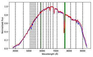
Figure 3: Normalized spectra of the target (blue line) and comparison (red line). The black dashed vertical lines show the wavelength bins used to generate the spectroscopic light curves. The green vertical lines show the location of the sodium and potassium features, which are both encompassed within narrow bins (30 and 50 Å respectively). Wavelengths outside of the range 4000–9000 Å were excluded due to low signal to noise.

4 Light curve fitting

With the white- and spectroscopic light curves created following the method presented in section 3, we were then able to fit models to these to extract the parameters of interest, namely the planet-to-star radius ratio $R_{\mathrm{P}}/R_{*}$.

To fit the white-light curve, we fitted Mandel & Agol (2002) analytic transit light curves with quadratic limb-darkening implemented through the Batman Python package (Kreidberg, 2015). These were fitted simultaneously with a Gaussian process (GP) to model the systematic noise. The fitted parameters determining the transit model were the time of midtransit ($T_{c}$), the inclination ($i$), the ratio of semi-major axis to stellar radius ($a/R_{*}$), the planet-to-star radius ratio $R_{\mathrm{P}}/R_{*}$, and the linear limb-darkening coefficient ($u1$). We chose to fix the quadratic limb-darkening coefficient ($u2$) to a theoretical value as the two limb-darkening coefficients are degenerate and, for the noise levels considered in our study, there is no advantage in fitting for both coefficients (Espinoza & Jordán, 2016). The period was held fixed to the value given in WASP-39b’s discovery paper (4.055259 days; Faedi et al. 2011). Uniform priors were placed on all these parameters to prevent unphysical values.

To calculate the theoretical limb-darkening coefficients used in the white- and spectroscopic light curve fits we used the Limb-Darkening Toolkit (LDTk) Python package (Parviainen & Aigrain, 2015). This uses phoenix stellar atmosphere models (Husser et al., 2013) with user-defined stellar parameters and uncertainties to calculate limb-darkening coefficients with uncertainties for a desired limb-darkening law. We used the stellar parameters and uncertainties listed in Faedi et al. (2011).

For the GP, we used the george Python package (Ambikasaran et al., 2014). GPs are now increasingly used in the exoplanet community, from detrending K2 photometry (Aigrain et al., 2016) to stellar variability analysis in radial velocity data (e.g., Haywood et al. 2014; Rajpaul et al. 2015) to transmission spectroscopy (e.g., Gibson et al. 2012a, b; Evans et al. 2015, 2017; Kirk et al. 2017, 2018; Louden et al. 2017; Parviainen2018). A GP is a nonparametric modeling technique that models the covariance in data. GPs are defined by kernels, which describe the characteristics of the covariance matrix, and hyperparameters, which, in this case, define the length scale and amplitude of the covariance.

We used six squared exponential kernels taking air mass, FWHM, the mean $x$ position of the stars on the CCD, the mean $y$ positions of the stars on the CCD, the mean sky background recorded at each star’s location, and time as input variables. Following the procedure of Evans et al. (2017, 2018), we standardized the GP inputs by subtracting the mean and dividing by the standard deviation for each input variable. This gives each input a mean of zero and standard deviation of unity, which helps the GP determine the inputs of importance for describing the noise characteristics. The x positions and sky background were obtained as functions of the dispersion direction during the extraction process (section 3) and therefore were binned in wavelength using the same bins as the spectra themselves. For the white-light curve, the $x$ positions and sky were integrated over the entire wavelength range. Each of these six kernels had an independent length scale ($\tau$) but shared a common amplitude ($a$). Following other studies using GPs (e.g., Evans et al., 2017, 2018; Gibson et al., 2017) we fitted for the natural logarithm of these hyperparameters and fitted for the inverse length scale ($1/\tau$), each with loose uniform priors. Finally, we also included a white-noise term in the GP to account for white-noise not accounted for by the photometric error bars. This resulted in 13 fit parameters for the white light curve.

To perform the fitting, we ran a Monte Carlo Markov chain (MCMC) using the emcee Python package (Foreman-Mackey et al., 2013). For all our light curve fits, we began by using a running median to clip any points that deviated by $>$4$\sigma$ from the median, which clipped at most one to two points per light curve, and then optimized the GP hyperparameters to the out-of-transit data to find the starting locations for the GP hyperparameters. The starting locations for all the transit light curve parameters were from the discovery paper (Faedi et al., 2011) other than $u1$ for which we used the value calculated by LDTk.

For the white-light curve, we ran the MCMC for 10,000 steps with 312 walkers ($24\times n_{p}$, where $n_{p}$ is the number of parameters) and calculated the 16th, 50th and 84th percentiles for each parameter after discarding the first 5000 steps as burn in. Following the george documentation, we then ran a second chain with the walkers initiated with a small scatter around these values for a further 10,000 steps with 432 walkers and again discarded the first 5000 steps.

Following the fit of the white-light curve, we fitted the spectroscopic light curves but this time with $a/R_{*}$, $T_{c}$ and inclination fixed to the result from the white-light curve fit. We again fixed $u2$ to values calculated by LDTk for our wavelength bins and fitted for $u1$ with uniform priors preventing unphysical values. This resulted in 10 fitted parameters per spectroscopic light curve. We then ran MCMCs to each light curve, following the same process as for the white-light curve but with 240 walkers as there were fewer fitted parameters.

5 Results of WHT data analysis

The fit to the white-light curve is shown in Figure 4 with the resulting parameters given in Table 1, which are consistent with the literature.

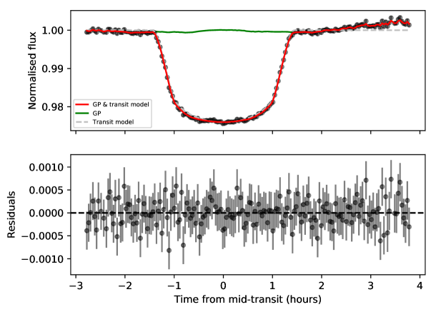
Figure 4: Plot of the fit using an analytic transit light curve and Gaussian process to the white-light curve of WASP-39. Top panel: the data are shown by the black error bars with the best-fitting model shown in red. The green line and gray dashed lines show the contributions of the GP systematics model and transit light curve model respectively. Bottom panel: the residuals of the best-fitting model (red line in upper panel).

Table 1: The parameters resulting from the fit to the white-light curve (Figure 4).

Parameter name (units)	Symbol	Value
Time of mid-transit (BJD)	$T_{c}$	$2457512.543848^{+0.000129}_{-0.000123}$
Inclination (degrees)	$i$	$87.83^{+0.2}_{-0.19}$
Ratio of semi-major axis to stellar radius	$a/R_{*}$	$11.5^{+0.19}_{-0.21}$
Ratio of planet to star radius	$R_{\mathrm{P}}/R_{*}$	$0.144636^{+0.001700}_{-0.001768}$
Linear limb-darkening coefficient	$u1$	$0.49\pm{0.06}$
Quadratic limb-darkening coefficient	$u2$ (fixed)	$0.08$

The fits to the spectroscopic light curves are shown in Figure 5 and the resulting $R_{\mathrm{P}}/R_{*}$ values given in Table 2.

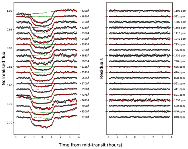
Figure 5: Left-hand panel: fits to our spectroscopic light curves combining quadratically limb-darkened analytic transit light curves with a GP. The black data points show the transit light curve for each wavelength bin, with the central wavelength of each bin given on the right-hand $y$-axis, and are offset in $y$ for clarity. The green line shows the best-fitting systematics (GP) model, and the red line shows the best-fitting systematics + analytic transit light curve model. Right-hand panel: the residuals for each fit shown in the left-hand panel, with the RMS of the residuals given on the right-hand $y$-axis. Note: the error bars are smaller than the data points.

5.1 The transmission spectrum

Our transmission spectrum resulting from the fits discussed in section 4 is plotted in Figure 6. This figure demonstrates our ability to achieve a precision of around one atmospheric scale height from a single transit, for wavelengths between 5500 and 7500 Å and bin widths $\geq 100$ Å.

Also plotted on Figure 6 are two forward models generated using exo-transmit (Kempton et al., 2017). A number of models with differing metallicities and Rayleigh scattering enhancements were generated but we only plot the best-fitting model (green line on Figure 6) and the model that Nikolov et al. (2016) found best matched their data set (yellow line on Figure 6). We also plot a Rayleigh scattering slope calculated using (Lecavelier Des Etangs et al., 2008)

$$\alpha H=\frac{dR_{P}}{d\ln\lambda}$$ (1)

where $\alpha=-4$ for Rayleigh scattering and $H$ is the atmospheric scale height. Also plotted on this transmission spectrum is a flat line corresponding to a gray cloud deck.

The models shown in Figure 6 do not account for stellar activity, which can introduce positive and negative slopes in transmission spectra depending on whether unocculted spots or faculae are present on the stellar surface (e.g., McCullough et al. 2014; Rackham et al. 2017). Instead, we present a retrieval analysis accounting for stellar activity in section 6, which shows that stellar activity plays a negligible role in the transmission spectrum of WASP-39b.

The $\chi^{2}$ values for each model are shown in Figure 6 and indicate that the transmission spectrum favors models with scattering slopes over a flat line. However, given we do not detect significant absorption by sodium or potassium, there is little difference in the goodness of fit between models. A subsolar metallicity atmosphere with enhanced Rayleigh scattering (green line) or pure Rayleigh scattering slope (blue line) is favored, although not significantly, over the solar metallicity atmosphere with enhanced Rayleigh scattering found by Nikolov et al. (2016) to best match their VLT data.

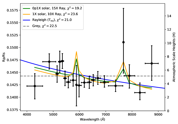
Figure 6: Our WHT transmission spectrum with forward models overplotted. The green and yellow models were generated using exo-transmit and correspond to subsolar and solar atmospheres with Rayleigh scattering slopes enhanced by factors of 15 and 10, respectively. The blue line corresponds to a Rayleigh scattering slope at the equilibrium temperature of the planet (1116 K; Faedi et al. 2011). The gray dashed line shows a flat transmission spectrum as resulting from a cloud deck. Each model has 19 degrees of freedom. Note that these models have been offset in $y$ to match the mean $R_{\mathrm{P}}/R_{*}$.

Table 2: The tabulated transmission spectrum from the analysis of our WHT data and as plotted in Figure 6.

Bin center	Bin width	$R_{\mathrm{P}}/R_{*}$	$u1$	$u2$
(Å)	(Å)
4300	600	$0.14225^{+0.00250}_{-0.00259}$	$0.85\pm 0.04$	$-0.07$
4850	500	$0.14714^{+0.00159}_{-0.00148}$	$0.66\pm 0.03$	$0.04$
5150	100	$0.14471^{+0.00161}_{-0.00171}$	$0.63\pm 0.05$	$0.01$
5250	100	$0.14714^{+0.00213}_{-0.00218}$	$0.65\pm 0.05$	$0.07$
5350	100	$0.14726^{+0.00151}_{-0.00149}$	$0.54\pm 0.04$	$0.07$
5450	100	$0.14381^{+0.00146}_{-0.00149}$	$0.57\pm 0.05$	$0.07$
5575	150	$0.14304^{+0.00110}_{-0.00116}$	$0.56\pm 0.04$	$0.09$
5760	220	$0.14342^{+0.00129}_{-0.00120}$	$0.51\pm 0.04$	$0.10$
5885	30	$0.14250^{+0.00390}_{-0.00425}$	$0.52^{+0.08}_{-0.09}$	$0.09$
5985	170	$0.14237^{+0.00199}_{-0.00232}$	$0.53\pm 0.06$	$0.11$
6185	230	$0.14294^{+0.00098}_{-0.00096}$	$0.47\pm 0.03$	$0.11$
6375	150	$0.14301^{+0.00126}_{-0.00123}$	$0.41\pm 0.04$	$0.12$
6525	150	$0.14345^{+0.00110}_{-0.00118}$	$0.37\pm 0.04$	$0.14$
6700	200	$0.14384^{+0.00134}_{-0.00126}$	$0.38^{+0.03}_{-0.04}$	$0.12$
6950	300	$0.14299^{+0.00134}_{-0.00098}$	$0.37\pm 0.03$	$0.13$
7375	550	$0.14229^{+0.00117}_{-0.00116}$	$0.36^{+0.03}_{-0.02}$	$0.13$
7675	50	$0.15105^{+0.00681}_{-0.00620}$	$0.49\pm 0.07$	$0.13$
7900	400	$0.14431^{+0.00222}_{-0.00248}$	$0.41\pm 0.04$	$0.13$
8300	400	$0.14092^{+0.00195}_{-0.00144}$	$0.34\pm 0.03$	$0.13$
8750	500	$0.14679^{+0.00357}_{-0.00342}$	$0.29\pm 0.05$	$0.13$

Figure 6 shows that the ‘enhancement’ of the Rayleigh scattering slope serves to shift the slope up in $R_{\mathrm{P}}/R_{*}$ rather than change the gradient of the slope. This effectively decreases the amplitude of the alkali absorption lines and is why these enhanced models provide a better fit to our data in Figure 6. Such an enhancement could be due to a high-altitude haze layer masking the pressure-broadened wings of the alkali wings that originate at lower altitudes. However, the amplitude of the alkali absorption lines can also be reduced by decreasing the metallicity of the atmosphere, decreasing the abundance of sodium and potassium. This introduces a degeneracy between the metallicity and the altitude of any haze layer. This is further explored in our retrieval analysis in section 6.

5.2 Comparison to VLT and HST

Because we used a binning scheme identical to that used by Nikolov et al. (2016), we can perform a direct comparison between our WHT results and their VLT results. This binning scheme is also nearly identical to the HST/STIS binning scheme of Fischer et al. (2016) and Sing et al. (2016), with an offset of 10 Å between the bin edges of our bins 8, 9, 10, 17, and 18 with the corresponding HST bins.

Figure 7 shows the comparison between our data and the studies of Nikolov et al. (2016), Fischer et al. (2016), and Sing et al. (2016). However, the Sing et al. (2016) data are taken from the Wakeford et al. (2018) study and is actually is a combination of data presented in Sing et al. (2016) and Nikolov et al. (2016). For this reason, we do not perform retrieval analysis on the Sing et al. (2016) data in section 6 as we perform an epoch-by-epoch analysis of the stellar activity, which is lost in the combination of data.

Figure 7 includes an offset applied to the VLT and HST/STIS data sets to account for small differences between the mean $R_{\mathrm{P}}/R_{*}$ values; however, the $R_{\mathrm{P}}/R_{*}$ values are within errors between each study. This figure shows that the optical data sets are consistent with one another and demonstrates the WHT’s ability to achieve precisions comparable to both the VLT and HST over the wavelength range 5500–8500 Å.

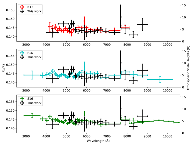
Figure 7: Top panel: a comparison between the transmission spectrum resulting from our WHT/ACAM data (black error bars) and the transmission spectrum resulting from Nikolov et al. (2016)’s VLT/FORS data (red error bars). Middle panel: a comparison between the transmission spectrum resulting from our WHT/ACAM data (black error bars) and the transmission spectrum resulting from Fischer et al. (2016)’s HST/STIS data (cyan error bars). Bottom panel: a comparison between the transmission spectrum resulting from our WHT/ACAM data (black error bars) and the transmission spectrum resulting from a combination of Sing et al. (2016)’s HST/STIS data (green error bars) and Nikolov et al. (2016)’s VLT data as presented in Wakeford et al. (2018). In this case, we have truncated the $x$-axis of Sing et al. (2016)’s data for clarity. Note: the VLT and HST spectra have had small offsets applied so their means are equal to our data.

5.3 The combined transmission spectrum of WASP-39b

Here we tabulate the combined transmission spectrum of WASP-39b. We report the transmission spectrum with no offset applied to the optical data, as the mean weighted optical transmission spectrum without an offset applied is consistent with the white-light $R_{\mathrm{P}}/R_{*}$ (Faedi et al., 2011).

We chose to use Wakeford et al. (2018)’s infrared reduction owing to the overlap in reduction approaches with Fischer et al. (2016), and the fact that it includes the HST/WFC3 G102 (0.8 – 1.0 $\mu$m) grism, which the Tsiaras et al. (2018) data set does not. Our combined transmission spectrum therefore includes HST/STIS data from Fischer et al. (2016), VLT/FORS data from Nikolov et al. (2016), HST/WFC3 data from Wakeford et al. (2018), Spitzer/IRAC data from Sing et al. (2016), and our WHT/ACAM optical data (Figure 6). The combined transmission spectrum spans the range 0.29–5.06 $\mu$m and is given in Table 3.

Table 3: The combined transmission spectrum of WASP-39b, using data from Fischer et al. (2016) (F16), Sing et al. (2016) (S16), Nikolov et al. (2016) (N16), Wakeford et al. (2018) (W18), in combination with the new optical transmission spectrum presented here (K19). The ‘source’ column indicates which data sets contributed to the values given in the transit depth column, which are a weighted average.

$\lambda$ ($\mu$m)	$\Delta\lambda$ ($\mu$m)	$R_{\mathrm{P}}/R_{*}$	Source	$\lambda$ ($\mu$m)	$\Delta\lambda$ ($\mu$m)	$R_{\mathrm{P}}/R_{*}$	Source
0.3355	0.0690	$0.14429\pm 0.00230$	F16	0.9082	0.0490	$0.14539\pm 0.00014$	W18
0.3825	0.0250	$0.14408\pm 0.00143$	F16	0.9625	0.1250	$0.14179\pm 0.00161$	F16
0.4032	0.0163	$0.14467\pm 0.00089$	F16	0.9572	0.0490	$0.14598\pm 0.00015$	W18
0.4300	0.0600	$0.14225^{+0.00250}_{-0.00259}$	K19	1.0062	0.0490	$0.14541\pm 0.00013$	W18
0.4180	0.0140	$0.14518\pm 0.00083$	F16, N16	1.0552	0.0490	$0.14457\pm 0.00015$	W18
0.4325	0.0150	$0.14637\pm 0.00077$	F16, N16	1.0920	0.0244	$0.14475\pm 0.00022$	W18
0.4450	0.0100	$0.14539\pm 0.00077$	F16, N16	1.1165	0.0244	$0.14596\pm 0.00024$	W18
0.4550	0.0100	$0.14412\pm 0.00072$	F16, N16	1.1391	0.0186	$0.14567\pm 0.00071$	W18
0.4650	0.0100	$0.14422\pm 0.00063$	F16, N16	1.1578	0.0186	$0.14625\pm 0.00041$	W18
0.4850	0.0500	$0.14714^{+0.00159}_{-0.00148}$	K19	1.1765	0.0186	$0.14611\pm 0.00043$	W18
0.4750	0.0100	$0.14453\pm 0.00062$	F16, N16	1.1951	0.0186	$0.14542\pm 0.00058$	W18
0.4850	0.0100	$0.14457\pm 0.00062$	F16, N16	1.2138	0.0186	$0.14500\pm 0.00068$	W18
0.4950	0.0100	$0.14442\pm 0.00065$	F16, N16	1.2325	0.0186	$0.14536\pm 0.00051$	W18
0.5050	0.0100	$0.14355\pm 0.00065$	F16, N16	1.2512	0.0186	$0.14576\pm 0.00064$	W18
0.5150	0.0100	$0.14390\pm 0.00061$	F16, N16, K19	1.2699	0.0186	$0.14417\pm 0.00040$	W18
0.5250	0.0100	$0.14529\pm 0.00068$	F16, N16, K19	1.2885	0.0186	$0.14628\pm 0.00076$	W18
0.5350	0.0100	$0.14434\pm 0.00058$	F16, N16, K19	1.3072	0.0186	$0.14582\pm 0.00060$	W18
0.5450	0.0100	$0.14416\pm 0.00072$	F16, N16, K19	1.3259	0.0186	$0.14663\pm 0.00051$	W18
0.5550	0.0100	$0.14437\pm 0.00098$	F16	1.3446	0.0186	$0.14663\pm 0.00047$	W18
0.5575	0.0150	$0.14467\pm 0.00062$	F16, N16, K19	1.3633	0.0186	$0.14687\pm 0.00066$	W18
0.5650	0.0100	$0.14558\pm 0.00083$	F16	1.3819	0.0186	$0.14733\pm 0.00058$	W18
0.5765	0.0230	$0.14561\pm 0.00048$	F16, N16, K19	1.4006	0.0186	$0.14749\pm 0.00059$	W18
0.5890	0.0040	$0.14915\pm 0.00125$	F16, N16, K19	1.4193	0.0186	$0.14674\pm 0.00050$	W18
0.5985	0.0170	$0.14534\pm 0.00055$	F16, N16, K19	1.4380	0.0186	$0.14788\pm 0.00065$	W18
0.6180	0.0240	$0.14470\pm 0.00050$	F16, N16, K19	1.4567	0.0186	$0.14772\pm 0.00076$	W18
0.6375	0.0150	$0.14438\pm 0.00056$	F16, N16, K19	1.4753	0.0186	$0.14803\pm 0.00063$	W18
0.6525	0.0150	$0.14472\pm 0.00067$	F16, N16, K19	1.4940	0.0186	$0.14718\pm 0.00068$	W18
0.6700	0.0200	$0.14366\pm 0.00063$	F16, N16, K19	1.5127	0.0186	$0.14653\pm 0.00067$	W18
0.6950	0.0300	$0.14362\pm 0.00049$	F16, N16, K19	1.5314	0.0186	$0.14655\pm 0.00072$	W18
0.7375	0.0550	$0.14401\pm 0.00048$	F16, N16, K19	1.5501	0.0186	$0.14656\pm 0.00052$	W18
0.7680	0.0060	$0.14713\pm 0.00116$	F16, N16, K19	1.5687	0.0186	$0.14607\pm 0.00068$	W18
0.7900	0.0400	$0.14616\pm 0.00067$	F16, N16, K19	1.5874	0.0186	$0.14519\pm 0.00071$	W18
0.8300	0.0400	$0.14227\pm 0.00130$	F16, K19	1.6061	0.0186	$0.14588\pm 0.00067$	W18
0.8750	0.0500	$0.14451\pm 0.00115$	F16, K19	1.6248	0.0186	$0.14596\pm 0.00084$	W18
0.8225	0.0244	$0.14435\pm 0.00031$	W18	1.6435	0.0186	$0.14441\pm 0.00061$	W18
0.8592	0.0490	$0.14482\pm 0.00019$	W18	3.5600	0.7600	$0.14438\pm 0.00061$	S16
				4.5000	1.1200	$0.14659\pm 0.00073$	S16

6 Retrieval analysis

In this section, we present retrieval analyses on different combinations of the data in the literature and our own data set. In particular, we wanted to test whether stellar activity could contribute to the supersolar metallicity atmosphere reported by Wakeford et al. (2018), as Pinhas et al. (2019) report a subsolar metallicity atmosphere for WASP-39b when accounting for stellar activity in their retrievals.

To determine the effects of differing stellar activity between the epochs of Fischer et al. (2016), Nikolov et al. (2016), Wakeford et al. (2018), and our observations, we ran separate retrievals on the three optical data sets (HST, VLT, and this data), each with the HST/WFC3 infrared data. We also ran retrievals on the HST/WFC3 data presented in Tsiaras et al. (2018), for which the authors found a subsolar water abundance. This is the same HST/WFC3 data as used in Wakeford et al. (2018) but reduced independently.

We chose to run retrievals on the optical data and infrared data combined as the optical data are needed to constrain the effects of stellar activity while the infrared data is needed to calculate the metallicity through the abundance of water. However, we also ran retrievals on the infrared data alone to test what effect the inclusion of optical data had.

We used the platon Python package (Zhang et al., 2019) to perform our retrieval analysis. platon is a new open-source Python code, which assumes equilibrium chemistry. This algorithm has been shown by Zhang et al. (2019) to produce results consistent with another independent algorithm, atmo (Goyal et al., 2018), which was the algorithm used by Wakeford et al. (2018). platon includes the ability to model the effects of stellar activity, parameterized by the temperature of the activity features, which can be cooler or hotter than the photosphere, and the filling factor. It then interpolates stellar atmosphere models and corrects the transit depth for the contribution of the activity region’s spectrum.

We ran retrievals on each combination of optical data (Fischer et al., 2016; Nikolov et al., 2016 and this work) with the infrared data of Wakeford et al. (2018). Additionally, we ran retrievals on the Wakeford et al. (2018) and Tsiaras et al. (2018) HST/WFC3 data alone to quantify the effects of including optical data and to see what impact the differing reduction pipelines had on the retrieved parameters.

platon does not fit for an offset in the transit depth between data gathered at different epochs or with different instruments. We tackled this offset in two separate ways to test how sensitive our results were to the difference in the baseline transit depth between the optical and infrared data. Firstly, for retrievals run on a single optical data set plus the WFC3 data, we normalized each optical data set to the infrared data by subtracting the difference in the mean transit depth of the optical data and infrared data. This assumes that stellar activity features have a negligible effect on infrared transmission spectra, as shown by Rackham et al. (2018) for FGK dwarfs, but spots can be seen in the infrared for very active stars (e.g., WASP-52b; Bruno et al. 2018). For the combined transmission spectrum, we took the weighted mean of the three optical data sets with no offset in the transit depth applied to the optical data as the weighted mean was consistent with the white-light transit depth (Faedi et al., 2011).

Given that platon does not support wavelengths shorter than 3000 Å, we had to amend the bluest bin of Fischer et al. (2016) from 2900–3700 Å to 3010–3700 Å. The retrieved parameters were the planet’s radius at a pressure of 1 bar ($R_{\mathrm{P}}$), equilibrium temperature ($T_{\mathrm{eq}}$), the logarithm of the atmospheric metallicity relative to the solar value ($\log Z$), and the C/O ratio. platon includes the treatment of clouds and hazes via the logarithm of the cloud-top pressure ($\log P_{\mathrm{cloud}}$), the logarithm of a factor that multiplies the scattering slope, raising the slope up and down in transit depth ($\log s$), and the gradient of the scattering slope ($\alpha$). These were all fitted parameters in our retrievals using platon. We also ran retrievals with each of these parameters plus the effects of stellar activity, parameterized through the active region’s temperature ($T_{\mathrm{active}}$) and covering fraction ($f_{\mathrm{active}}$).

We placed wide, uniform priors on all parameters retrieved by platon (Table 4). We used the nested sampling algorithm to explore the parameter space with 1000 live points, as recommended by the documentation (Zhang et al., 2019). Depending on the data set used, the nested sampling algorithm took between $\sim$15,000 and $\sim$35,000 likelihood evaluations before convergence.

Table 4: The prior ranges and parameters used for the retrievals using platon. Some of the parameter ranges were defined using values from the discovery paper (F11; Faedi et al., 2011). Note that not all retrievals were run using all parameters (see Table 5 for which parameters were included for which data set).

Parameter	Units	Prior
Planet radius at 1 bar ($R_{\mathrm{P}}$)	$R_{\mathrm{J}}$	Uniform ($0.9\times R_{\mathrm{P}}$(F11), $1.1\times R_{\mathrm{P}}$(F11))
Equilibrium temperature ($T_{\mathrm{eq}}$)	K	Uniform ($0.5\times T_{\mathrm{eq}}$(F11), $1.5\times T_{\mathrm{eq}}$(F11))
Metallicity ($\log Z/Z_{\odot}$)	-	Uniform (-1, 3)
C/O ratio	-	Uniform (0.05, 2.0)
Cloud-top pressure ($\log P_{\mathrm{cloud}}$)	Pa	Uniform (-0.99, 5)
Scattering factor ($\log s$)	-	Uniform (-10, 10)
Scattering gradient ($\alpha$)	-	Uniform (-4, 10)
Unocculted spot/facula temperature ($T_{\mathrm{active}}$)	K	Uniform ($T_{\mathrm{eff}}$(F11) - 2500, $T_{\mathrm{eff}}$(F11) + 2500)
Unocculted spot/facula covering fraction ($f_{\mathrm{active}}$)	-	Uniform (0, 0.5)

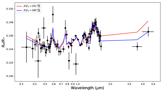
Figure 9: The platon retrievals run on the combined transmission spectrum, incorporating data from five different studies (Table 3). The red line shows the retrieved model without fitting for stellar activity, and the blue line shows the retrieved model accounting for stellar activity. The legend shows the metallicity, relative to solar, retrieved by each model.

The resulting values for each retrieval using platon are shown in Table 5 with retrieved model atmospheres shown in Figures 8 and 9. The key findings of these retrievals are that platon finds a highly supersolar metallicity atmosphere regardless of which data set is used, and stellar activity has a negligible effect on both the C/O ratio and the metallicity, with the exception being the retrieval performed on the Tsiaras et al. (2018) data set alone. In this case, when including stellar activity, the metallicity increases from $245^{+86}_{-59}\times$ solar to $407^{+130}_{-105}\times$ solar, although with large uncertainties.

The fits to the combined transmission spectrum (Table 5 and Figure 9) retrieve a metallicity of $282^{+65}_{-58}\times$ and $331^{+86}_{-74}\times$ solar depending on whether or not stellar activity is taken into account. The nested sampling algorithm calculates the Bayesian evidences (which we call $\ln\chi$ so as not to be confused with the metallicity, $\log Z$), which marginally favor the retrieval with stellar activity with $\Delta\ln\chi=3$.

Wakeford et al. (2018) also retrieved a supersolar metallicity atmosphere, of $151^{+48}_{-46}\times$ solar (1.2$\sigma$ lower than the value we find), while Tsiaras et al. (2018) found a subsolar water abundance. However, our retrievals on the Tsiaras et al. (2018) data alone recover a highly supersolar metallicity atmosphere, which differs significantly from the finding of these authors. Our retrieval using platon is also in disagreement with the results of Pinhas et al. (2019) who find a subsolar metallicity atmosphere for WASP-39b when running a retrieval on the Sing et al. (2016) and Tsiaras et al. (2018) data. These discrepancies are discussed further in section 7.2.

Furthermore, when considering Figure 8, it is clear that the study of Tsiaras et al. (2018) found a significantly offset and lower amplitude water feature than the study of Wakeford et al. (2018). The reason for this difference is unclear but could be related to a different treatment of systematic noise and different system parameters between the two studies. However, despite the differing amplitudes, our retrievals on the Tsiaras et al. (2018) data using platon (Zhang et al., 2019) also find supersolar metallicities. We considered whether our supersolar metallicities were dependent on the degeneracy between the volume mixing ratio of water, which sets the atmospheric metallicity, and both the reference pressure and radius (e.g., Lecavelier Des Etangs et al., 2008; Griffith, 2014; Heng & Kitzmann, 2017; Pinhas et al., 2019).

To test the effects of the cloud-top pressure and reference radius on the derived metallicities using platon, we also ran a retrieval on the Tsiaras et al. (2018) data alone with these parameters fixed to the values reported in that study. We find that in this case that fixing the cloud-top pressure and reference radius does not change the conclusion of a highly supersolar metallicity atmosphere (Table 5). We discuss this further in section 7.1.

While the C/O ratio varies depending on which data set is used (Table 5), the retrieved parameters are broadly consistent with the solar C/O ratio of 0.54, when using optical and infrared data and are subsolar when using the infrared data alone.

The lack of impact caused by stellar activity is perhaps not unexpected as both the C/O and metallicity are driven by the infrared data, which is not as affected by stellar activity, for which we only have one epoch of data. This can be seen by the consistency between the $\log Z$ values retrieved from the infrared data alone and infrared + optical data. This result implies that stellar activity is not the reason behind the supersolar metallicity atmosphere we derive for WASP-39b. This is also in agreement with the star being inactive as determined through a lack of photometric variation (Faedi et al., 2011; Fischer et al., 2016) and weak Ca II H and K emission ($\log R^{\prime}_{\mathrm{HK}}=-4.97\pm 0.06$; Mancini et al., 2018).

Table 5: PLATON retrieval results for the parameters as defined in the text. Retrievals were run on different combinations of Wakeford et al. (2018) (W18), Tsiaras et al. (2018) (T18), Fischer et al. (2016) (F16), Nikolov et al. (2016) (N16) and this work (K19). Note: platon fits for the cloud top pressure in units of Pa, but we have converted these to units of bar here.

Data set	$R_{\mathrm{P}}$ ($R_{\mathrm{J}}$)	$T_{\mathrm{eq}}$ (K)	$\log Z$	C/O	$\log P_{\mathrm{cloud}}$ (bar)	$\log s$	$\alpha$	$T_{\mathrm{active}}$ (K)	$f_{\mathrm{active}}$
W18 w/o activity	$1.23^{+0.00}_{-0.00}$	$880^{+99}_{-66}$	$2.31^{+0.14}_{-0.16}$	$0.32^{+0.20}_{-0.18}$	$-1.07^{+0.71}_{-0.86}$	$0.47^{+0.34}_{-0.32}$	-	-	-
W18 w/ activity	$1.23^{+0.01}_{-0.02}$	$970^{+229}_{-127}$	$2.35^{+0.15}_{-0.17}$	$0.38^{+0.19}_{-0.22}$	$-1.23^{+0.78}_{-0.86}$	$0.49^{+0.34}_{-0.33}$	-	$4665^{+758}_{-1427}$	$0.04^{+0.07}_{-0.03}$
T18 w/o activity	$1.21^{+0.01}_{-0.01}$	$1180^{+175}_{-148}$	$2.39^{+0.13}_{-0.12}$	$0.21^{+0.19}_{-0.11}$	$-2.28^{+1.44}_{-1.21}$	$4.02^{+0.45}_{-0.91}$	-	-	-
T18 w/ activity	$1.17^{+0.03}_{-0.02}$	$1246^{+221}_{-187}$	$2.61^{+0.12}_{-0.13}$	$0.26^{+0.22}_{-0.15}$	$-3.06^{+1.81}_{-0.75}$	$-2.27^{+4.88}_{-5.00}$	-	$3478^{+1127}_{-370}$	$0.13^{+0.04}_{-0.05}$
T18 w/o activity	1.24 (fixed)	$893^{+115}_{-96}$	$2.72^{+0.11}_{-0.12}$	$0.11^{+0.11}_{-0.04}$	-0.14 (fixed)	$-3.44^{+4.56}_{-4.44}$	-	-	-
T18 w/ activity	1.24 (fixed)	$871^{+113}_{-86}$	$2.74^{+0.11}_{-0.10}$	$0.12^{+0.12}_{-0.05}$	-0.14 (fixed)	$-3.43^{+4.29}_{-4.32}$	-	$5325^{+87}_{-420}$	$0.06^{+0.20}_{-0.05}$
N16+W18 w/o activity	$1.23^{+0.00}_{-0.01}$	$1036^{+77}_{-71}$	$2.43^{+0.11}_{-0.14}$	$0.46^{+0.17}_{-0.22}$	$-1.85^{+0.65}_{-0.56}$	$-3.65^{+3.32}_{-4.35}$	$2.87^{+4.66}_{-4.52}$	-	-
N16+W18 w/activity	$1.23^{+0.01}_{-0.01}$	$1011^{+93}_{-57}$	$2.35^{+0.14}_{-0.18}$	$0.52^{+0.15}_{-0.28}$	$-1.38^{+0.51}_{-0.70}$	$-4.10^{+3.26}_{-3.93}$	$3.20^{+4.41}_{-4.69}$	$4422^{+902}_{-1177}$	$0.03^{+0.08}_{-0.02}$
F16+W18 w/o activity	$1.23^{+0.01}_{-0.01}$	$1076^{+99}_{-111}$	$2.41^{+0.11}_{-0.13}$	$0.46^{+0.19}_{-0.27}$	$-1.12^{+0.75}_{-0.81}$	$1.66^{+0.54}_{-0.79}$	$4.12^{+1.92}_{-1.18}$	-	-
F16+W18 w/activity	$1.21^{+0.01}_{-0.02}$	$1212^{+122}_{-109}$	$2.39^{+0.10}_{-0.12}$	$0.55^{+0.11}_{-0.20}$	$-1.91^{+1.19}_{-0.65}$	$-0.62^{+1.64}_{-5.51}$	$4.52^{+3.45}_{-4.20}$	$3696^{+1317}_{-508}$	$0.06^{+0.03}_{-0.02}$
K19+W18 w/o activity	$1.23^{+0.00}_{-0.00}$	$897^{+110}_{-71}$	$2.30^{+0.15}_{-0.17}$	$0.34^{+0.19}_{-0.18}$	$-1.31^{+0.86}_{-0.89}$	$0.28^{+0.87}_{-1.20}$	$7.07^{+2.08}_{-3.72}$	-	-
K19+W18 w/ activity	$1.23^{+0.01}_{-0.02}$	$975^{+219}_{-114}$	$2.34^{+0.15}_{-0.18}$	$0.35^{+0.20}_{-0.19}$	$-1.73^{+1.09}_{-0.86}$	$-0.12^{+1.16}_{-5.36}$	$6.01^{+2.84}_{-5.09}$	$4944^{+444}_{-1552}$	$0.04^{+0.09}_{-0.03}$
Combined w/o activity	$1.23^{+0.00}_{-0.01}$	$1110^{+62}_{-61}$	$2.52^{+0.10}_{-0.11}$	$0.43^{+0.15}_{-0.21}$	$-2.00^{+1.31}_{-0.71}$	$-0.53^{+1.66}_{-5.62}$	$4.51^{+3.55}_{-3.80}$	-	-
Combined w/ activity	$1.20^{+0.01}_{-0.01}$	$1133^{+108}_{-75}$	$2.45^{+0.09}_{-0.10}$	$0.25^{+0.19}_{-0.14}$	$-2.17^{+0.94}_{-0.42}$	$-2.51^{+2.55}_{-4.99}$	$4.07^{+3.89}_{-4.96}$	$3257^{+709}_{-267}$	$0.05^{+0.02}_{-0.01}$

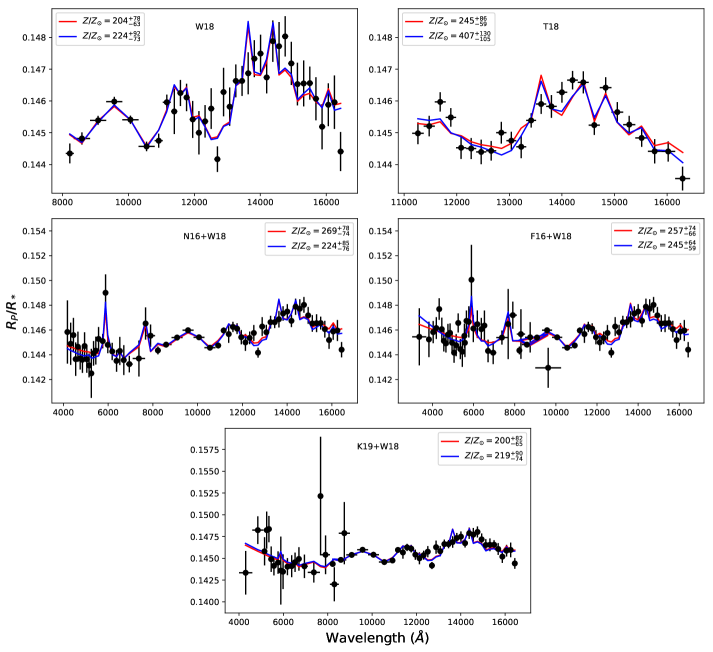
Figure 8: Results from the running of platon retrievals. Each panel is labeled according to which combination of data sets is used. In each panel, the black points show the data, the solid red line shows the retrieved model without accounting for stellar activity, and the blue line shows the retrieval accounting for stellar activity. The legends give the atmospheric metallicity relative to solar for all models.

7 Discussion

7.1 On the discrepancies in the literature

As noted throughout this work, there have been significantly different water abundances, and hence metallicities, reported for WASP-39b in the literature. The reported water abundances are given in Table 6 and are taken from Wakeford et al. (2018), Tsiaras et al. (2018), Fisher & Heng (2018), and Pinhas et al. (2019). We also include the metallicities that these water abundances correspond to, assuming a scaled solar composition atmosphere and a solar water abundance of $3.6\times 10^{-4}$, as used by Wakeford et al. (2018).

Table 6 highlights how the retrieved water abundances differ by over four orders of magnitude in the literature. This includes orders-of-magnitude differences between retrievals run on identical data sets (Fisher & Heng, 2018; Tsiaras et al., 2018 and Table 5). In order for us to make conclusions about the planet’s atmospheric metallicity, we must first consider the causes for the large differences in the literature.

Table 6: The reported logarithmic water abundances ($\log X_{\mathrm{H_{2}O}}$) as reported in the literature and how these compare to the solar value, along with the data sets used in the retrievals (using the same paper references as in Table 3).

Study	Data sets used	$\log X_{\mathrm{H_{2}O}}$	$Z/Z_{\odot}$
Wakeford et al. (2018), equilibrium chemistry	S16, N16, W18*	-	$151^{+48}_{-46}$
Wakeford et al. (2018), disequilibrium chemistry	S16, N16, W18*	$-1.37^{+0.05}_{-0.13}$	$117^{+14}_{-30}$
Tsiaras et al. (2018)	T18**	$-5.94\pm 0.61$	$0.003^{+0.010}_{-0.002}$
Fisher & Heng (2018)	T18**	$-2.3^{+0.40}_{-0.67}$	$14^{+21}_{-11}$
Pinhas et al. (2019)	S16, T18**	$-4.07^{+0.72}_{-0.78}$	$0.24^{+1.00}_{-0.20}$
This work	N16, F16, S16, W18*, K19	-	$282^{+65}_{-58}$
*using HST/WFC3 grisms G102 and G141.
**using HST/WFC3 grism G141 only.

In the retrievals used in section 6, we used isothermal temperature–pressure profiles. platon (Zhang et al., 2019) has the ability to use non-isothermal temperature–pressure profiles both for forward modeling of transmission spectra and retrievals of eclipse spectra but not yet for retrievals of transmission spectra. In a retrieval analysis of simulated JWST data, Rocchetto et al. (2016) showed that assuming an isothermal temperature–pressure profile can lead to retrieved abundances that are typically an order of magnitude too large and with underestimated uncertainties. Rocchetto et al. (2016) found that a parameterized temperature–pressure profile, however, recovered abundances that were generally within 1$\sigma$ of the true values. Conversely, Heng & Kitzmann (2017) demonstrated that isothermal temperature–pressure profiles were able to produce transmission spectra that matched numerical calculations with non-isothermal profiles, when applied to HST/WFC3 data.

Concerning the temperature–pressure profiles used in the literature, both our retrievals and those of Tsiaras et al. (2018) assumed isothermal temperature–pressure profiles. Wakeford et al. (2018) fitted for the temperature–pressure profile in their retrieval and found that parameterized profiles were unnecessary to fit their data, instead finding the retrieved temperature–pressure profile to be isothermal. Pinhas et al. (2019) fitted for the temperature–pressure profile using the parametric profile of Madhusudhan & Seager (2009) and found a non-isothermal temperature–pressure profile and a subsolar metallicity atmosphere. Finally, Fisher & Heng (2018) found no strong evidence for a non-isothermal temperature–pressure profile and recovered a supersolar water abundance.

Given the lack of correlation between the treatment of the temperature–pressure profile and the water abundances reported in the literature, it is not obvious how much of an effect this has. Instead, the discrepancies could be related to a degeneracy between the reference pressure, reference radius and the abundance of water (e.g., Lecavelier Des Etangs et al., 2008; Griffith, 2014; Heng & Kitzmann, 2017; Pinhas et al., 2019), although Welbanks & Madhusudhan (2019) find this degeneracy to have little effect on abundance estimates.

A direct comparison between the reference radii and pressures reported in the literature is more difficult. This is because these values are typically defined and treated differently for each study. However, to test the effect of this degeneracy, we also ran a retrieval on the Tsiaras et al. (2018) data alone with the reference radius and cloud-top pressure fixed to the values reported in that study. However, despite doing this, we still recover a highly supersolar metallicity (Table 5). Instead, we find that the equilibrium temperature recovered from this fit is lower than when fitting for the radius and pressure. The reason for this change in temperature is perhaps related to our assumption of an isothermal temperature–pressure profile.

It is also possible that the differing results in the literature result from whether equilibrium chemistry was assumed during the retrieval analysis. The retrievals of Tsiaras et al. (2018), Fisher & Heng (2018) and Pinhas et al. (2019) do not assume equilibrium chemistry and instead they retrieve for the water abundance directly. The water abundances retrieved by these studies vary from highly subsolar to marginally supersolar (Table 6). The retrievals presented here, however, assume equilibrium chemistry and recover highly supersolar metallicities for all literature data sets (Tables 5 and 6). Wakeford et al. (2018) present the results of retrievals assuming equilibrium and free (disequilibrium) chemistry. These both result in highly supersolar metallicities of $151^{+48}_{-46}\times$ and $117^{+14}_{-30}\times$ solar (Table 6), respectively. This suggests that the assumption of equilibrium vs. disequilibrium chemistry is not the driving factor behind the discrepancies in the literature. However, we intend to perform the same analysis presented here but without the assumption of equilibrium chemistry in a future work.

Despite the above discussion that the assumption of equilibrium chemistry is unlikely to be the cause of the discrepancies, we should also consider the priors placed on the water volume mixing ratios used in the literature. Tsiaras et al. (2018), Fisher & Heng (2018), and Pinhas et al. (2019) all used log-uniform priors, bounded by $10^{-8}$ – $10^{-1}$, $10^{-13}$ – 1, and $10^{-12}$ – $10^{-2}$ respectively. Wakeford et al. (2018) do not state the prior ranges used, but the water volume mixing ratio they derive using their free chemistry model ($-1.37^{+0.05}_{-0.13}$) is excluded by the bounds of Pinhas et al. (2019). The upper bounds are motivated by the fact that water should be a trace species in a gas-giant atmosphere (particularly one as low density as WASP-39b). However, the location of this bound should be explored when considering a planet with a large-amplitude water feature.

The above discussion highlights the impact that different assumptions and fitting methods have on the abundances of retrieved species, which are heavily model dependent.

7.2 The atmospheric metallicity of WASP-39b

In this section, we discuss the implications of the supersolar metallicity derived by platon. We are encouraged to pursue this interpretation as our analysis includes more data sets than any previous study of WASP-39b.

As detailed in section 6, we retrieve a supersolar metallicity atmosphere for all data sets, including the Tsiaras et al. (2018) data set. Our retrieval on the combined transmission spectrum found a $282^{+65}_{-58}\times$ solar metallicity atmosphere when taking into account stellar activity, as was marginally preferred.

However, the optical transmission spectra, when taken alone and when compared with forward models, are best represented by solar or even subsolar metallicities (section 5.1 and Fischer et al., 2016; Nikolov et al., 2016). The metallicities in the optical data are determined through the amplitude of the alkali absorption features, which are degenerate with the altitude of clouds and hazes (as discussed in section 5.1). It is therefore possible that the optical data underestimate the actual metallicity of the atmosphere, which is better constrained by the amplitude of the water feature in the infrared. In addition, the condensation of alkali chlorides (which occurs at $\sim$800 K, Burrows & Sharp, 1999) could remove sodium and potassium from the upper, cooler atmosphere. This condensation could result in the muted alkali absorption features we see without invoking a low-metallicity atmosphere (Figure 6).

Given WASP-39b’s very supersolar metallicity, it sits above the trend observed for the solar system giant planets (Wakeford et al., 2018). This begs the question of how WASP-39b would accumulate such a supersolar metallicity atmosphere. In our retrievals using platon (section 6 and Table 5), we also recovered the C/O ratios, which were broadly consistent with a solar C/O ratio. Given WASP-39 is a G star with solar metallicity (Faedi et al., 2011), we will assume that this means that WASP-39b’s C/O ratio is stellar. The combination of a stellar C/O ratio and super-stellar metallicity suggests that a large amount of icy material polluted the atmosphere postformation (Öberg et al., 2011). Indeed, disk formation followed by migration can lead to $10\times$ solar metallicities (Madhusudhan et al., 2014), but this is still an order of magnitude less than we derive (Table 5).

As an additional challenge to such a metal-rich atmosphere, Thorngren & Fortney (2019) calculated the maximum atmospheric metallicity of WASP-39b to be $54.5\times$ solar, significantly less than what we find and Wakeford et al. (2018) find. Thorngren & Fortney (2019) calculated the bulk metallicity of the planet’s interior from its mass and radius combined with an evolutionary model which describes the planet’s radius as a function of time (Thorngren et al., 2016). Thorngren & Fortney (2019) used the bulk metallicity of the interior as an upper limit to the atmospheric metallicity, as the atmosphere cannot be more metal rich than the interior postformation due to Rayleigh-Taylor instabilities and convection.

However, Thorngren & Fortney (2019) note that the maximum metallicity they calculate could be underestimated if the planet’s interior is hotter than expected, if the planet is tidally heated, or is much younger than the models, although they predict these effects to be minimal for hot Jupiters. This makes the supersolar metallicity atmosphere of WASP-39b hard to explain, unless there is ongoing ablation of metal-rich material in its atmosphere. In any case, the atmosphere must be well mixed in order to be so rich in metals, suggesting a minimal core or composition gradient (Thorngren & Fortney, 2019).

8 Conclusions

We present a new optical transmission spectrum of the Saturn-mass planet WASP-39b. Our optical transmission spectrum was acquired through the LRG-BEASTS transmission spectroscopy survey and is in good agreement with previous VLT and HST/STIS spectra. This study further demonstrates the WHT’s ability to achieve transmission spectra with precisions comparable to both HST and VLT over a wavelength range 5500–8500 Å.

We performed a retrieval analysis using different combinations of all published transmission spectra of this planet. Our retrievals, which assume equilibrium chemistry, recover a highly supersolar metallicity atmosphere. This supports Wakeford et al. (2018)’s finding of a supersolar metallicity atmosphere but is at odds with the studies of Tsiaras et al. (2018), Fisher & Heng (2018) and Pinhas et al. (2019). If the atmospheric metallicity of WASP-39b is as supersolar as our retrievals suggest, this poses a challenge to our understanding of the formation of this planet as its atmospheric metallicity is significantly enhanced relative to its interior.

We show that the orders-of-magnitude discrepancies regarding the atmospheric metallicity of WASP-39b in the literature are not due to stellar activity, as we demonstrate this to have a minimal effect. Instead, they are more likely due to differing retrieval approaches, in particular the treatment of the reference pressure and planetary radius.

This work highlights how differing assumptions during retrieval analyses can lead to water abundances that differ by orders of magnitude, in this case over four. This is a concern as WASP-39b is one of the very best targets for transmission spectroscopy. We must explore and understand such biases before we can claim to accurately retrieve the abundances of smaller planets with JWST data.

9 Software and third party data repository citations

References

- Aigrain et al. (2016) Aigrain, S., Parviainen, H., & Pope, B. J. S. 2016, MNRAS, 459, 2408, doi: 10.1093/mnras/stw706
- Ambikasaran et al. (2014) Ambikasaran, S., Foreman-Mackey, D., Greengard, L., Hogg, D. W., & O’Neil, M. 2014, ArXiv e-prints. https://arxiv.org/abs/1403.6015
- Arcangeli et al. (2018) Arcangeli, J., Desert, J.-M., Line, M. R., et al. 2018, ArXiv e-prints. https://arxiv.org/abs/1801.02489
- Armstrong et al. (2016) Armstrong, D. J., de Mooij, E., Barstow, J., et al. 2016, Nature Astronomy, 1, 0004, doi: 10.1038/s41550-016-0004
- Astropy Collaboration et al. (2013) Astropy Collaboration, Robitaille, T. P., Tollerud, E. J., et al. 2013, A&A, 558, A33, doi: 10.1051/0004-6361/201322068
- Barstow et al. (2017) Barstow, J. K., Aigrain, S., Irwin, P. G. J., & Sing, D. K. 2017, ApJ, 834, 50, doi: 10.3847/1538-4357/834/1/50
- Benn et al. (2008) Benn, C., Dee, K., & Agócs, T. 2008, in Proc. SPIE, Vol. 7014, Ground-based and Airborne Instrumentation for Astronomy II, 70146X
- Benneke & Seager (2012) Benneke, B., & Seager, S. 2012, ApJ, 753, 100, doi: 10.1088/0004-637X/753/2/100
- Boffin et al. (2015) Boffin, H., Blanchard, G., Gonzalez, O., et al. 2015, The Messenger, 159, 6. https://arxiv.org/abs/1502.03172
- Bruno et al. (2018) Bruno, G., Lewis, N. K., Stevenson, K. B., et al. 2018, AJ, 156, 124, doi: 10.3847/1538-3881/aac6db
- Burrows & Sharp (1999) Burrows, A., & Sharp, C. M. 1999, ApJ, 512, 843, doi: 10.1086/306811
- Charbonneau et al. (2002) Charbonneau, D., Brown, T. M., Noyes, R. W., & Gilliland, R. L. 2002, ApJ, 568, 377, doi: 10.1086/338770
- Crossfield & Kreidberg (2017) Crossfield, I. J. M., & Kreidberg, L. 2017, AJ, 154, 261, doi: 10.3847/1538-3881/aa9279
- Espinoza & Jordán (2016) Espinoza, N., & Jordán, A. 2016, MNRAS, 457, 3573, doi: 10.1093/mnras/stw224
- Espinoza et al. (2019) Espinoza, N., Rackham, B. V., Jordán, A., et al. 2019, MNRAS, 482, 2065, doi: 10.1093/mnras/sty2691
- Evans et al. (2015) Evans, T. M., Aigrain, S., Gibson, N., et al. 2015, MNRAS, 451, 680, doi: 10.1093/mnras/stv910
- Evans et al. (2017) Evans, T. M., Sing, D. K., Kataria, T., et al. 2017, Nature, 548, 58, doi: 10.1038/nature23266
- Evans et al. (2018) Evans, T. M., Sing, D. K., Goyal, J. M., et al. 2018, AJ, 156, 283, doi: 10.3847/1538-3881/aaebff
- Faedi et al. (2011) Faedi, F., Barros, S. C. C., Anderson, D. R., et al. 2011, A&A, 531, A40, doi: 10.1051/0004-6361/201116671
- Fischer et al. (2016) Fischer, P. D., Knutson, H. A., Sing, D. K., et al. 2016, ApJ, 827, 19, doi: 10.3847/0004-637X/827/1/19
- Fisher & Heng (2018) Fisher, C., & Heng, K. 2018, MNRAS, 481, 4698, doi: 10.1093/mnras/sty2550
- Foreman-Mackey et al. (2013) Foreman-Mackey, D., Hogg, D. W., Lang, D., & Goodman, J. 2013, PASP, 125, 306, doi: 10.1086/670067
- Fu et al. (2017) Fu, G., Deming, D., Knutson, H., et al. 2017, ApJ, 847, L22, doi: 10.3847/2041-8213/aa8e40
- Gibson et al. (2012a) Gibson, N. P., Aigrain, S., Roberts, S., et al. 2012a, MNRAS, 419, 2683, doi: 10.1111/j.1365-2966.2011.19915.x
- Gibson et al. (2017) Gibson, N. P., Nikolov, N., Sing, D. K., et al. 2017, MNRAS, 467, 4591, doi: 10.1093/mnras/stx353
- Gibson et al. (2012b) Gibson, N. P., Aigrain, S., Pont, F., et al. 2012b, MNRAS, 422, 753, doi: 10.1111/j.1365-2966.2012.20655.x
- Goyal et al. (2018) Goyal, J. M., Mayne, N., Sing, D. K., et al. 2018, MNRAS, 474, 5158, doi: 10.1093/mnras/stx3015
- Griffith (2014) Griffith, C. A. 2014, Philosophical Transactions of the Royal Society of London Series A, 372, 20130086, doi: 10.1098/rsta.2013.0086
- Haywood et al. (2014) Haywood, R. D., Collier Cameron, A., Queloz, D., et al. 2014, MNRAS, 443, 2517, doi: 10.1093/mnras/stu1320
- Heng (2016) Heng, K. 2016, ApJ, 826, L16, doi: 10.3847/2041-8205/826/1/L16
- Heng & Kitzmann (2017) Heng, K., & Kitzmann, D. 2017, MNRAS, 470, 2972, doi: 10.1093/mnras/stx1453
- Hoeijmakers et al. (2018) Hoeijmakers, H. J., Ehrenreich, D., Heng, K., et al. 2018, Nature, 560, 453, doi: 10.1038/s41586-018-0401-y
- Hoeijmakers et al. (2019) Hoeijmakers, H. J., Ehrenreich, D., Kitzmann, D., et al. 2019, arXiv e-prints, arXiv:1905.02096. https://arxiv.org/abs/1905.02096
- Hunter (2007) Hunter, J. D. 2007, Computing In Science & Engineering, 9, 90, doi: 10.1109/MCSE.2007.55
- Husser et al. (2013) Husser, T.-O., Wende-von Berg, S., Dreizler, S., et al. 2013, A&A, 553, A6, doi: 10.1051/0004-6361/201219058
- Jones et al. (2001) Jones, E., Oliphant, T., Peterson, P., et al. 2001, SciPy: Open source scientific tools for Python. http://www.scipy.org/
- Kempton et al. (2017) Kempton, E. M.-R., Lupu, R., Owusu-Asare, A., Slough, P., & Cale, B. 2017, PASP, 129, 044402, doi: 10.1088/1538-3873/aa61ef
- Kirk (2018) Kirk, J. 2018, PhD thesis, University of Warwick. https://wrap.warwick.ac.uk/111014/
- Kirk et al. (2017) Kirk, J., Wheatley, P. J., Louden, T., et al. 2017, MNRAS, 468, 3907, doi: 10.1093/mnras/stx752
- Kirk et al. (2016) —. 2016, MNRAS, 463, 2922, doi: 10.1093/mnras/stw2205
- Kirk et al. (2018) —. 2018, MNRAS, 474, 876, doi: 10.1093/mnras/stx2826
- Kreidberg (2015) Kreidberg, L. 2015, Publications of the Astronomical Society of the Pacific, 127, 1161, doi: 10.1086/683602
- Kreidberg et al. (2014) Kreidberg, L., Bean, J. L., Désert, J.-M., et al. 2014, Nature, 505, 69, doi: 10.1038/nature12888
- Lecavelier Des Etangs et al. (2008) Lecavelier Des Etangs, A., Pont, F., Vidal-Madjar, A., & Sing, D. 2008, A&A, 481, L83, doi: 10.1051/0004-6361:200809388
- Louden et al. (2017) Louden, T., Wheatley, P. J., Irwin, P. G. J., Kirk, J., & Skillen, I. 2017, MNRAS, 470, 742, doi: 10.1093/mnras/stx984
- MacDonald & Madhusudhan (2017) MacDonald, R. J., & Madhusudhan, N. 2017, MNRAS, 469, 1979, doi: 10.1093/mnras/stx804
- Madhusudhan (2012) Madhusudhan, N. 2012, ApJ, 758, 36, doi: 10.1088/0004-637X/758/1/36
- Madhusudhan et al. (2014) Madhusudhan, N., Amin, M. A., & Kennedy, G. M. 2014, ApJ, 794, L12, doi: 10.1088/2041-8205/794/1/L12
- Madhusudhan & Seager (2009) Madhusudhan, N., & Seager, S. 2009, ApJ, 707, 24, doi: 10.1088/0004-637X/707/1/24
- Mallonn et al. (2016) Mallonn, M., Bernt, I., Herrero, E., et al. 2016, MNRAS, 463, 604
- Mancini et al. (2018) Mancini, L., Esposito, M., Covino, E., et al. 2018, A&A, 613, A41, doi: 10.1051/0004-6361/201732234
- Mandel & Agol (2002) Mandel, K., & Agol, E. 2002, ApJ, 580, L171, doi: 10.1086/345520
- McCullough et al. (2014) McCullough, P., Crouzet, N., Deming, D., & Madhusudhan, N. 2014, ApJ, 791, 55
- Morley et al. (2015) Morley, C. V., Fortney, J. J., Marley, M. S., et al. 2015, ApJ, 815, 110, doi: 10.1088/0004-637X/815/2/110
- Nikolov et al. (2016) Nikolov, N., Sing, D. K., Gibson, N. P., et al. 2016, ApJ, 832, 191, doi: 10.3847/0004-637X/832/2/191
- Nikolov et al. (2018) Nikolov, N., Sing, D. K., Fortney, J. J., et al. 2018, Nature, 557, 526, doi: 10.1038/s41586-018-0101-7
- Öberg et al. (2011) Öberg, K. I., Murray-Clay, R., & Bergin, E. A. 2011, ApJ, 743, L16, doi: 10.1088/2041-8205/743/1/L16
- Parviainen & Aigrain (2015) Parviainen, H., & Aigrain, S. 2015, MNRAS, 453, 3821, doi: 10.1093/mnras/stv1857
- Parviainen et al. (2017) Parviainen, H., Palle, E., Chen, G., et al. 2017, ArXiv e-prints. https://arxiv.org/abs/1709.01875
- Pinhas & Madhusudhan (2017) Pinhas, A., & Madhusudhan, N. 2017, MNRAS, 471, 4355, doi: 10.1093/mnras/stx1849
- Pinhas et al. (2019) Pinhas, A., Madhusudhan, N., Gandhi, S., & MacDonald, R. 2019, MNRAS, 482, 1485, doi: 10.1093/mnras/sty2544
- Pinhas et al. (2018) Pinhas, A., Rackham, B. V., Madhusudhan, N., & Apai, D. 2018, MNRAS, 480, 5314, doi: 10.1093/mnras/sty2209
- Pont et al. (2008) Pont, F., Knutson, H., Gilliland, R. L., Moutou, C., & Charbonneau, D. 2008, MNRAS, 385, 109, doi: 10.1111/j.1365-2966.2008.12852.x
- Pont et al. (2013) Pont, F., Sing, D. K., Gibson, N. P., et al. 2013, MNRAS, 432, 2917, doi: 10.1093/mnras/stt651
- Rackham et al. (2017) Rackham, B., Espinoza, N., Apai, D., et al. 2017, ApJ, 834, 151, doi: 10.3847/1538-4357/aa4f6c
- Rackham et al. (2018) Rackham, B. V., Apai, D., & Giampapa, M. S. 2018, arXiv e-prints, arXiv:1812.06184. https://arxiv.org/abs/1812.06184
- Rajpaul et al. (2015) Rajpaul, V., Aigrain, S., Osborne, M. A., Reece, S., & Roberts, S. 2015, MNRAS, 452, 2269, doi: 10.1093/mnras/stv1428
- Rocchetto et al. (2016) Rocchetto, M., Waldmann, I. P., Venot, O., Lagage, P. O., & Tinetti, G. 2016, ApJ, 833, 120, doi: 10.3847/1538-4357/833/1/120
- Sing et al. (2016) Sing, D. K., Fortney, J. J., Nikolov, N., et al. 2016, Nature, 529, 59, doi: 10.1038/nature16068
- Spake et al. (2018) Spake, J. J., Sing, D. K., Evans, T. M., et al. 2018, Nature, 557, 68, doi: 10.1038/s41586-018-0067-5
- Stevenson (2016) Stevenson, K. B. 2016, ApJ, 817, L16, doi: 10.3847/2041-8205/817/2/L16
- Thorngren & Fortney (2019) Thorngren, D., & Fortney, J. J. 2019, ApJ, 874, L31, doi: 10.3847/2041-8213/ab1137
- Thorngren et al. (2016) Thorngren, D. P., Fortney, J. J., Murray-Clay, R. A., & Lopez, E. D. 2016, ApJ, 831, 64, doi: 10.3847/0004-637X/831/1/64
- Tsiaras et al. (2018) Tsiaras, A., Waldmann, I. P., Zingales, T., et al. 2018, AJ, 155, 156, doi: 10.3847/1538-3881/aaaf75
- Van Der Walt et al. (2011) Van Der Walt, S., Colbert, S. C., & Varoquaux, G. 2011, Computing in Science & Engineering, 13, 22
- Wakeford & Sing (2015) Wakeford, H. R., & Sing, D. K. 2015, A&A, 573, A122, doi: 10.1051/0004-6361/201424207
- Wakeford et al. (2017) Wakeford, H. R., Visscher, C., Lewis, N. K., et al. 2017, MNRAS, 464, 4247, doi: 10.1093/mnras/stw2639
- Wakeford et al. (2018) Wakeford, H. R., Sing, D. K., Deming, D., et al. 2018, AJ, 155, 29, doi: 10.3847/1538-3881/aa9e4e
- Welbanks & Madhusudhan (2019) Welbanks, L., & Madhusudhan, N. 2019, AJ, 157, 206, doi: 10.3847/1538-3881/ab14de
- Zahnle et al. (2009) Zahnle, K., Marley, M. S., Freedman, R. S., Lodders, K., & Fortney, J. J. 2009, ApJ, 701, L20, doi: 10.1088/0004-637X/701/1/L20
- Zhang et al. (2019) Zhang, M., Chachan, Y., Kempton, E. M. R., & Knutson, H. A. 2019, PASP, 131, 034501, doi: 10.1088/1538-3873/aaf5ad