Superfluidity fraction of few bosons in an annular geometry in the presence of a rotating weak link

Abstract

We report a beyond mean-field calculation of mass current and superfluidity fraction for a system of few bosons confined in a ring geometry in the presence of a rotating weak link induced by a potential barrier. We apply the Multiconfiguration Hartree Method for bosons to compute the ground state of the system and show the average superfluidity fraction for a wide range of interaction strength and barrier height, highlighting the behavior of density correlation functions. The decrease of superfluidity fraction due to the increase of barrier height is found whereas the condensation fraction depends exclusively on the interaction strength, showing the independence of both phenomena.

I Introduction

The concepts of superfluidity Khalatnikov (1965); Leggett (1998, 1999) and Bose-Einstein condensation Anderson et al. (1995); Pethick and Smith (2008) have dominated the research of cold bosonic systems. The presence of one do not necessarily imply the other, whereas superfluidity is related to dissipationless flow due to a minimum required energy to create excitations, Bose-Einstein condensation is characterized by a single macroscopically occupied state. Superfluid systems with very small condensation fraction around $10\%$, like liquid Helium, are widely known Penrose and Onsager (1956); Sears et al. (1982), thereby characterizing independent effects.

Nevertheless, many reports explore the superfluidity features of a Bose-Einstein condensate (BEC), as dilute cold bosonic gases are able to present both phenomena simultaneously Raman et al. (1999). Specially, persistent flow, hallmark of superfluidity, has been reported for a BEC trapped in a ring shape format early in Ryu et al. (2007) and later in Ramanathan et al. (2011) in the presence of a tunable weak link. This boosted the interest to quantitatively study all the properties for the system due to a possible connection and quantum analogy with superconducting quantum interference devices (SQUID) Clark and Braginski (2004), that was experimentally implemented Ryu et al. (2013) generating Josephson junctions Albiez et al. (2005).

Many works studied several properties on imposing rotation for a BEC confined in a ring shape geometry, observing hysteresis (“swallow tail loops”) Mueller (2002); Eckel et al. (2014); Baharian and Baym (2013); Syafwan et al. (2016), excitation mechanisms Wright et al. (2013); Kunimi and Danshita (2019); Kumar et al. (2017), spin superflow Kim et al. (2017); Beattie et al. (2013) and superfluid fraction Cooper and Hadzibabic (2010). Although the theoretical studies rely mostly on the Gross-Pitaevskii (GP) equation that set a clear limitation on controlling the interactions to suppress the depletion from the condensate Lopes et al. (2017); Chang et al. (2016), this has changed in the past few years with the development of novel methods able to compute many-body observables and assure correctness for a wider range of interaction values.

The employment of new methods pave a way to study independently the condensation phenomena and the superfluidity for a system of cold bosonic atoms and to sweep a wider range for interaction strength since depletion is included on the description. Moreover, they enable us a deep understanding of the physical system through new many-body quantities unseen in the mean field formalism, like correlations that has gained importance due to experimental measures in the past decade for cold atomic clouds Navon et al. (2015); Naraschewski and Glauber (1999); Dall et al. (2013); Hodgman et al. (2017).

Specifically, the Multi-Configuration Time Dependent Hartree method for Bosons (MCTDHB) Alon et al. (2008) has dragged attention for its quite straightforward generalization of the GP equation, since it is still based on variational principle but with more single-particle states (also known as orbitals) the atoms can occupy, therefore allowing the expansion of the many-body state in a configuration basis (Fock states) with each possible configuration expressed by a well-defined occupation number of the single-particle states. This procedure truncate the Hilbert space, whereas the coefficients of the basis expansion and the orbitals are determined by minimizing the action, enforcing an optimized basis. The MCTDHB has shown to be a powerful tool for many applications like bosons in optical lattices Roy et al. (2018), quench dynamics Lode et al. (2015) and other applications Nguyen et al. (2019); Klaiman and Cederbaum (2016); Lode (2016) as well as a version for fermions Fasshauer and Lode (2016).

In the present report, we study beyond mean field the superfluidity fraction of a gas of bosons at zero temperature in the presence of a tunnable weak link moving in a periodic system (an effective ring), for a small number of atoms, using the MCTDHB to exploit strong interactions and to show the loss of the superfluidity fraction under a wide range of the physical parameters. Explanations for the superfluid properties are studied here through correlation of the bosonic field operator in the absence of rotation, which is directly related to the tunneling amplitude in the neighborhood of the barrier, therefore allowing a prediction if the atoms would be dragged when some rotation is applied.

II Model and methods

The specific form of a barrier is generally unknown from an experimental perspective, though we must be able to define it through its thickness and height. As most of the experiments use lasers to physically implement a barrier Ramanathan et al. (2011), the height in the model plays the principal role as it is directly related to laser intensity, and the thickness can be fixed in a first moment. Indeed, an approach based on Dirac delta function for the barrier has been reported Cominotti et al. (2014), which implies zero thickness. In any case, for a barrier rotating with velocity $v$, in the laboratory frame we thus have the one-body term of the Hamiltonian in the general form

$$\hat{h}(t)=-\frac{\hbar^{2}}{2m}\frac{\partial^{2}}{\partial\bar{x}^{2}}+U(\bar{x}-vt)\ ;\quad\bar{x}\in(-\pi R,\pi R],$$ (1)

for a ring of radius $R$. The two-body part is assumed to be described by an effective contact interaction $V(\bar{x}-\bar{x}^{\prime})=g_{1\mathrm{D}}\delta(\bar{x}-\bar{x}^{\prime})$, where $g_{1\mathrm{D}}$ is related to the transverse harmonic trap frequency and the scattering length of the atoms. Using a unitary transformation to move to the rotating frame, the time dependence of Eq. (1) is removed, resulting in the following many-body Hamiltonian in the second quantized formalism

$$\mathcal{H}=\int_{-\pi R}^{\pi R}\!\!\!\!\!\mathrm{d}x\ \Psi^{\dagger}(x)\left[\frac{\hbar^{2}}{2m}\left(i\frac{\partial}{\partial x}+\frac{mv}{\hbar}\right)^{2}+U(x)\right]\Psi(x)\ +\\ \frac{g_{1\mathrm{D}}}{2}\int\!\!\!\mathrm{d}x\ \Psi^{\dagger}(x)\Psi^{\dagger}(x)\Psi(x)\Psi(x),$$ (2)

where $x=\bar{x}-vt$.

The MCTDHB is developed assuming a truncated Hilbert space where the many-body state is a superposition of all possible configurations $N_{c}$ of $N$ particles distributed over $M$ single-particle states, such that we can write

$$|\Psi(t)\rangle\ \doteq\ \sum_{\alpha=1}^{N_{c}}C_{\alpha}(t)|\vec{n}^{(\alpha)}\rangle,\quad N_{c}=\binom{N+M-1}{M-1},$$ (3)

where a valid configuration $|\vec{n}^{(\alpha)}\rangle$ is a Fock state where $\sum_{i}^{M}n_{i}^{(\alpha)}=N$, $\forall\alpha\in\mathbb{N}\ |\ 1\leq\alpha\leq N_{c}$. Furthermore, the occupation number refers to a set of single-particle states $\{\phi_{k}(x,t)\ |\ \int\!\!\mathrm{d}x\phi_{l}^{*}(x,t)\phi_{k}(x,t)=\delta_{lk},\forall k,l=1,...,M\}$. Using this Ansatz, the time-dependent equations can be extracted from a minimization of the action with respect to the coefficients $C_{\alpha}$ in Eq. (3) and the single-particle state, with the action defined by

$$\mathcal{S}\Big{[}\mathbf{C},\{\phi_{k},\phi_{k}^{*}\}\Big{]}=\int\!\!\!\mathrm{dt}\bigg{[}\langle\Psi(t)|\dot{\Psi}(t)\rangle\ -\ \langle\Psi(t)|\mathcal{H}|\Psi(t)\rangle\ \\ -\sum_{k,l=1}^{M}\mu_{kl}(t)\langle\phi_{k}|\phi_{l}\rangle_{t}\bigg{]},$$ (4)

where the $\mu_{kl}$ are introduced as Lagrangian multipliers to maintain orthonormality of the single-particle states. The variational principle conducts to $M$ nonlinear coupled partial differential equations for the set $\{\phi_{k}(x,t)\}$ and a system of $N_{c}$ ordinary differential equation for the coefficients $C_{\alpha}$ Meyer et al. (2009); Alon et al. (2008). It is worth mentioning that the GP equation is a special case where we have just one possible configuration $|\vec{n}\rangle=|N,0,...,0\rangle$, that yield for the macroscopically occupied orbital $\phi(x,t)$ the equation

$$i\hbar\frac{\partial\phi}{\partial t}=\Big{[}\hat{h}^{\prime}+g(N-1)|\phi(x,t)|^{2}\Big{]}\phi(x,t),$$ (5)

with $\hat{h}^{\prime}=\hbar^{2}/2m\left(i\partial/\partial x+mv/\hbar\right)^{2}+U(x)$ the one-body Hamiltonian in the rotating frame.

For numerical simulation purposes, we assume the following system of units: length measured in units of $(\pi R)$, probability/particle density in unis of $(\pi R)^{-1}$ and energy by $\hbar\zeta$ where $\zeta=(\hbar/2m\pi^{2}R^{2})$. Moreover, we introduce the dimensionless parameters $\Omega=mRv/\hbar$ and $\gamma=2m\pi Rg_{1\mathrm{D}}/\hbar^{2}$. All these transformations yield the following orthonormal condition for the set of orbitals: $\int_{-1}^{1}\!\!\mathrm{d}x\phi_{l}^{*}(x,t)\phi_{k}(x,t)=\delta_{lk}$. Here we developed our own codes to solve the MCTDHB equations with periodic boundary conditions. Our codes were extensively tested, matching results of the examples of the code available in Ref. Lode et al. , that has produced many results until now Fasshauer and Lode (2016); Lode (2016); Klaiman and Cederbaum (2016); Nguyen et al. (2019); Lode et al. (2015).

III Periodicity in energy spectrum and definition of superfluidity fraction

In the absence of a barrier, the single-particle energy levels as function of $\Omega$ are parabolas given by $E_{j}/(\hbar\zeta)=(j-\Omega)^{2}\pi^{2}$, each one defined by the winding number of the phase ($j$), centered at $\Omega_{j}=j$, and crossing each other at $\tilde{\Omega}_{j}=(j+1/2)~{}$Baharian and Baym (2013).

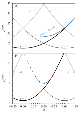
Figure 1: (Color online) Energy per particle from GP equation as a function of $\Omega$ for different winding numbers ($j$) with (A) $\gamma(N-1)=50$ and (B) $\gamma(N-1)=10$. In both figures the soliton solutions energy are depicted in blue, whose connect the parabolas with $j=0$ to $j=1$, shown by dotted and full line respectively. Other values of winding numbers are shown in gray.

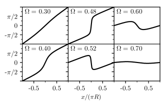
Figure 2: Phase profile of soliton solution for some values of $\Omega$ corresponding to the red dots in 1. An abrupt transition occurs at $\Omega=0.5$ that implies a transition in the winding numbers.

As a first approach, we use the GP equation once the interaction is included in the description. In this case, still in the absence of the barrier, there are two kinds of analytical solutions, one with constant density, which results in the same energy of single-particle case, with the addition of an interaction contribution, yielding $E^{(GP)}_{j}/(\hbar\zeta)=(j-\Omega)^{2}\pi^{2}+\gamma(N-1)/4$ as average energy per particle. The other is a soliton given in terms of Jacobi elliptic functions Carr et al. (2000); Sato et al. (2016) that exists for a finite range of values of $\Omega$, whereas the extension of this range depends on the interaction strength. Fig. 1 shows an energy landscape of the analytical solutions of the GP equation with the soliton solution energy connecting two parabolas from constant density solutions, where the dotted lines have winding number 1 and the filled line 0.

From Fig. 2 we check that the soliton solution is responsible for the transition between different winding numbers and a discontinuity occurs in $\Omega=0.5$ in its phase. Moreover, the soliton connects the values of angular momentum Muñoz Mateo et al. (2015) and this connection between the two lines is related to an hysteretic behavior by the presence of a “swallow-tail” loop Muñoz Mateo et al. (2015); Mueller (2002); Eckel et al. (2014); Baharian and Baym (2013). The soliton branch in Fig. 1 is an excited state Baharian and Baym (2013), however, it will not be discussed here, since the aim of the present work is to measure the superfluidity fraction for the ground state. In addition, Fig. 1 reveals that the ground state energy has a periodic behavior with respect to the rotation $\Omega$, with kinks where the parabolas cross each other at $\tilde{\Omega}_{j}=(j+1/2)$. This periodic structure remains even in the presence of a barrier as will be shown later. An important fact is that we can relate the mass current circulation with the energy, and use this periodicity to understand what happens with the current under action of fast rotating barriers.

Here we start a derivation of mass current by looking at the time variation of the number of atoms within the range $[x_{1},x_{2}]\subseteq[-\pi R,\pi R]$, as

$$\frac{\mathrm{d}}{\mathrm{d}t}\int_{x_{1}}^{x_{2}}\!\!\!\!\!\!\mathrm{d}x\ \langle\Phi(t)|\hat{\Psi}^{\dagger}(x)\hat{\Psi}(x)|\Phi(t)\rangle=\frac{i}{\hbar}\int_{x_{1}}^{x_{2}}\!\!\!\!\!\!\mathrm{d}x\ \langle\big{[}\mathcal{H},\hat{\Psi}^{\dagger}(x)\hat{\Psi}(x)\big{]}\rangle_{t},$$ (6)

where $\langle\cdot\rangle_{t}$ means the expectation value for an arbitrary many-body state $|\Phi(t)\rangle$. Using Eq. (2) with the usual commutation relation for the boson field operator $[\hat{\Psi}(x),\hat{\Psi}^{\dagger}(x^{\prime})]=\delta(x-x^{\prime})$ to evaluate the commutator of the Hamiltonian with the density operator, the only terms that contribute are those carrying a derivative, and yields

$$\big{[}\hat{\Psi}^{\dagger}(x)\hat{\Psi}(x),\mathcal{H}\big{]}=-\frac{\hbar^{2}}{2m}\left(\hat{\Psi}^{\dagger}(x)\frac{\partial^{2}\hat{\Psi}(x)}{\partial x^{2}}-\frac{\partial^{2}\hat{\Psi}^{\dagger}(x)}{\partial x^{2}}\hat{\Psi}(x)\right)\\ +i\hbar v\left(\hat{\Psi}^{\dagger}(x)\frac{\partial\hat{\Psi}(x)}{\partial x}+\frac{\partial\hat{\Psi}^{\dagger}(x)}{\partial x}\hat{\Psi}(x)\right).$$ (7)

It is straightforward to factor out the derivative with respect to $x$, and further using Eq. (7) in Eq. (6) yields

$$\frac{\mathrm{d}}{\mathrm{d}t}N([x_{1},x_{2}];t)=-\Big{[}\langle\hat{J}(x_{2})\rangle_{t}-\langle\hat{J}(x_{1})\rangle_{t}\Big{]}$$ (8)

where $N([x_{1},x_{2}];t)=\int_{x_{1}}^{x_{2}}\mathrm{d}x\langle\Phi(t)|\hat{\Psi}^{\dagger}(x)\hat{\Psi}(x)|\Phi(t)\rangle$ is introduced and the particle number current operator $\hat{J}(x)$ is given by

$$\hat{J}(x)=-\frac{i\hbar}{2m}\left(\hat{\Psi}^{\dagger}(x)\frac{\partial\hat{\Psi}(x)}{\partial x}-\frac{\partial\hat{\Psi}^{\dagger}(x)}{\partial x}\hat{\Psi}(x)\right)\\ -v\hat{\Psi}^{\dagger}(x)\hat{\Psi}(x).$$ (9)

The reduced single-particle density matrix (1-RDM) defined by $n^{(1)}(x,x^{\prime};t)\doteq\langle\hat{\Psi}^{\dagger}(x^{\prime})\hat{\Psi}(x)\rangle_{t}$ Naraschewski and Glauber (1999) has as a set of eigenvalues and eingenstates defined by the solution of $\int_{-\pi R}^{\pi R}\!\mathrm{d}x\ n^{(1)}(x,x^{\prime};t)\psi(x^{\prime},t)=\mathcal{N}(t)\psi(x,t)$, with $\mathcal{N}(t)$ the average occupation number in the eigenstate $\psi(x,t)$, here also called as natural orbital. Using these natural orbitals to express the reduced single-particle density matrix $n^{(1)}(x,x^{\prime};t)$ allows us to express the current as a superposition, $\langle\hat{J}(x)\rangle_{t}=\sum_{k}j_{k}(x,t)$, where

$$j_{k}=-\left[\frac{i\hbar}{2m}\left(\psi_{k}^{*}\frac{\partial\psi_{k}}{\partial x}-\psi_{k}\frac{\partial\psi_{k}^{*}}{\partial x}\right)+v|\psi_{k}|^{2}\right]\mathcal{N}_{k},$$ (10)

with the position and time arguments omitted.

For the ground state, the current $\langle\hat{J}(x)\rangle_{t}$ must be independent of position and time, because the density is not time-dependent. If we further average it over a period in the counter direction of the barrier velocity, yields

$$\langle\rho_{s}\rangle(v)=\tau\frac{1}{2\pi R}\int_{\pi R}^{-\pi R}\!\!\!\!\!\mathrm{d}x\ \left(\frac{\langle\hat{J}\rangle}{N}\right),$$ (11)

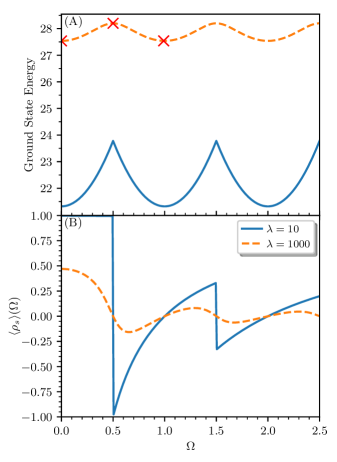
Figure 3: (Color online) Ground state energy and current fraction for 11 particles as a function of dimensionless rotation velocity $\Omega$ in the rotating frame. The ground state energy remains periodic as it was in Fig. 1 but with a different landscape depending on the barrier height $\lambda$, and this periodicity implies a decrease on the current fraction for fast rotating barriers. Dimensionless interaction strength parameter used was $\gamma=10$.

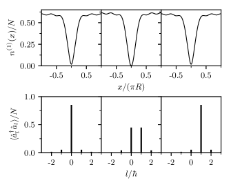
Figure 4: Probability distribution for position(upper panel) where $n^{(1)}(x)\equiv n^{(1)}(x,x)=\langle\hat{\Psi}^{\dagger}(x)\hat{\Psi}(x)\rangle$ and angular momentum distribution(lower panel) for barrier height $\lambda=1000$. From left to right $\Omega=0,0.5,1.0$, corresponding to red crosses in Fig. 3, and as used before $\gamma=10$ for 11 particles.

where $\tau=2\pi R/v$ is the period of barrier rotation. This quantify the mean fraction of particles that go through the counter direction of the barrier in its period, that is from $\pi R$ to $-\pi R$ indicated by the limits of integration taken. Therefore, if $\langle\rho_{s}\rangle(v)$ takes the value 1, means a perfect superfluid since all the particles are flowing with velocity $-v$ in the rotating frame, that is, they remain at rest for a observer in the laboratory frame. Relations with other observables can be established, for instance, using the average momentum per particle

$$\langle\rho_{s}\rangle(v)=\left(1-\frac{\langle\hat{p}\rangle}{mv}\right),\quad\hat{p}=-\frac{i\hbar}{N}\int_{-\pi R}^{\pi R}\!\!\!\!\!\!\!\!\mathrm{d}x\ \Psi^{\dagger}(x)\frac{\partial}{\partial x}\Psi(x),$$ (12)

and a relation with the energy, by taking the derivative with respect to the barrier velocity

$$\langle\rho_{s}\rangle(v)=\frac{1}{Nmv}\frac{\partial E}{\partial v},\quad E=\langle\mathcal{H}\rangle.$$ (13)

The equation above can also be identified by the ratio between the moment of inertia of the atoms and the moment of inertia of a rigid body. Using $v=\omega R$, yields

$$\langle\rho_{s}\rangle(\omega)=\frac{1}{NmR^{2}}\left(\frac{1}{\omega}\frac{\partial E}{\partial\omega}\right)=\frac{I(\omega)}{I_{\mathrm{cl}}}.$$ (14)

Superfluidity fraction at rest (or simply superfluidity fraction), denoted here by $\langle\rho_{s}\rangle_{0}$ can be defined by taking the limit of $v\rightarrow 0$ in any of the forms (11),(12),(13) or (14) and was studied in this way in previous works Cooper and Hadzibabic (2010); Leggett (1999, 1970, 1998). With the dimensionless system of units and parameters introduced in the end of section II, we have a suitable expression for numerical calculations

$$\langle\rho_{s}\rangle(\Omega)=\left(\frac{1}{2\pi^{2}N\Omega}\frac{\partial E}{\partial\Omega}\right),\ \langle\rho_{s}\rangle_{0}=\lim_{\Omega\rightarrow 0}\langle\rho_{s}\rangle(\Omega).$$ (15)

Here we use the MCTDHB to find the ground state through imaginary time propagation for several parameters, and we first study the effect of rotation. Fig. 3 illustrate the behavior of the energy in panel (A) and the current fraction in panel (B) as function of dimensionless barrier frequency $\Omega$ for two different barrier heights, where the specific form used in Eq. (1) was

$$U(x)=\left\{\begin{array}[]{lcl}\displaystyle(\hbar\zeta\lambda)\cos^{2}{\left(\frac{x}{2R\sigma}\right)}&\mathrm{if}&|x|\leq\pi R\sigma\\ 0&\mathrm{if}&\ \pi R\geq|x|>\pi R\sigma\end{array}\right.,$$ (16)

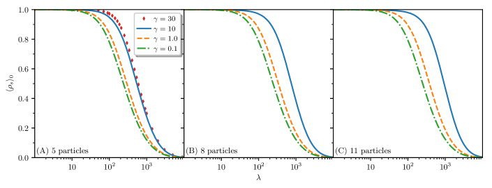
Figure 5: (Color online) Decrease of superfluidity fraction for different number of particles and interaction strength($\gamma$) due to increasing of the barrier height($\lambda$). All the cases share the common feature to be a perfect superfluid as the barrier becomes vanishing small, soon or later depending on the number of particles and interaction strength. For very high barriers all particles are dragged together, imposing a rigid body rotation to the system.

where $\lambda$ denotes the barrier height in dimensionless units and the width of the barrier was taken fixed $\sigma=0.1$ .

The energy of the ground state in Fig. 3(A) has a period 1 with respect to dimensionless rotation frequency for both cases of weak and strong barriers, while the difference relies on the maximum that occurs at $\Omega_{j}=j$, that is peaked or smooth. The current fraction shows a periodic behavior with a damped amplitude as function of $\Omega$ in Fig. 3(B), due to the periodicity of energy, where according to Eq. (15), the amplitude is damped by a factor of $1/\Omega$. In the regions where $\langle\rho_{s}\rangle(\Omega)<1$ the average momentum must increase together with the barrier velocity by Eq. (12). Indeed, that is what occurs in lower panel of Fig. 4 that shows the angular momentum distribution fo some values of $\Omega$. Moreover, there is a critical dependence of the superfluid fraction on the barrier height, where Fig. 3 shows that, as $\Omega$ goes to zero, $\langle\rho_{s}\rangle(\Omega)$ becomes as smaller as higher is the barrier. This fact will be explored in the following.

IV Decrease of superfluidity fraction due to increase of the barrier height

Numerical calculations of superfluidity fraction was carried out here using Eq. (13), finding the ground state by imaginary time propagation for $\Omega=0$ and $\Omega=0.02$, to approximate the derivative in $\Omega=0.01$ and so get $\langle\rho_{s}\rangle(0.01)$. As showed by Fig. 3 the slope of current fraction goes to zero as $\Omega\rightarrow 0$, and therefore we use the value at $\Omega=0.01$ as the proper superfluidity fraction, assuming the difference of $\langle\rho_{s}\rangle_{0}-\langle\rho_{s}\rangle(0.01)$ to be close to zero. To assure this method is valid, we compare with the result using Eq. (12) at $\Omega=0.02$, to check if there is no appreciable(less than 1%) variation on the estimation of superfluidity fraction using a constant extrapolation of $\langle\rho_{s}\rangle(0.01)$.

In Fig. 5, we show the decrease of superfluid fraction for an increase in the barrier height for the form in Eq. (16), using different number of particles and interaction strength. Here the tunneling of particles through the barrier is as harder as higher is the barrier, thereby the system acquires momentum easily for stronger barriers because it drags almost every particle with it. This easy momentum gain for very strong barriers is responsible for the loss of superfluidity fraction $\langle\rho_{s}\rangle_{0}$. The superfluidity fraction decreases more rapidly for fewer particles and lower interaction strength, however, the number of particles and strenght of interactions have a small impact in the form of the curves of $\langle\rho_{s}\rangle_{0}$ as a function of $\lambda$.

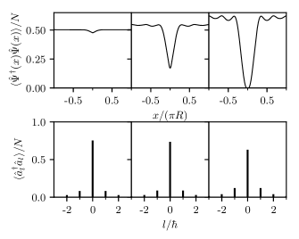
Figure 6: Probability distribution of position(upper panel) and angular momentum(lower panel) for 5 particles, $\gamma=30$ and different barrier heights $\lambda=10,200,10000$ in the left, center and right column respectively, in the absence of rotation $\Omega=0$. The density distribution vanishes for $\lambda>10^{3}$ at the peak of the barrier in $x=0$, despite there is just a slight increase on the width of the angular momentum distribution.

As can be seen in upper panel of Fig. 6, the barrier height $\lambda$ influence mostly the density at its peak, while the effect over the momentum distribution is a slight increase in its variance, but preserving $\langle\hat{L}\rangle=0$, as can be checked by the lower panel. This effect can also be seen in Fig. 3, from which for $\lambda=10$ the barrier has a critical value $\Omega=0.5$ to start to move the particles, whereas for $\lambda=1000$ it drags more easily the atoms since there $\langle\rho_{s}\rangle_{0}\approx 0.46$.

	1	10	30
11	0.9936 / 0.9920	0.92 / 0.89	-
8	0.9946 / 0.9935	0.92 / 0.88	-
5	0.9962 / 0.9956	0.91 / 0.88	0.75 / 0.70

Table 1: maximum/minimum condensation fraction numbers given by the highest eingenvalue of $n^{(1)}(x,x^{\prime})$, over the set of values of $\lambda$ in Fig. 5. The maximum and minimum values for each case have little influence from the barrier height whereas the superfluid fraction maximum and minimum values goes from 1 to 0 respectively. For $\gamma=30$ we were able to perform the calculations only for 5 particles due to our code limitations.

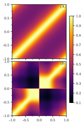
Figure 7: (Color online) $|g^{(1)}(x,x^{\prime})|^{2}$ mapped to colors in the ring, for 5 particles and $\gamma=30$, where the horizontal and vertical axes represent $x$ and $x^{\prime}$ values in units of $\pi R$, respectively. Values of barrier height used are $\lambda=10$ in (A) and $\lambda=10^{4}$ in (B) but sharing the same color scale.

It is worth noting that this loss of superfluidity fraction due to increase in the barrier height is not related with the condensation fraction. As can be inferred from table 1, the condensation fraction depends mostly on the interaction strength and is minimally affected by the barrier height, particularly for small values of $\gamma$.

Being able to investigate many-body quantities that are unreachable using the GP equation, we further investigate how the tunneling amplitude is affected by the barrier height, that is the transition amplitude for the system to move a particle from $x$ to $x^{\prime}$. This can be achieved by $|\langle\hat{\Psi}^{\dagger}(x^{\prime})\hat{\Psi}(x)\rangle|^{2}$ weighted by the probabilities to find the particles in respective positions given by $n^{(1)}(x)$ and $n^{(1)}(x^{\prime})$. This is directly related to the first order normalized correlation function defined by Naraschewski and Glauber (1999); Sakmann et al. (2008)

$$g^{(1)}(x,x^{\prime})=\frac{\langle\hat{\Psi}^{\dagger}(x^{\prime})\hat{\Psi}(x)\rangle}{\sqrt{n^{(1)}(x)n^{(1)}(x^{\prime})}}.$$ (17)

The values of $g^{(1)}$ shall be drastically affected by the barrier and must have an abrupt variation as $xx^{\prime}>0$ changes to $xx^{\prime}<0$, since the tunneling must be much harder if the shorter distance between two points has the barrier between them. Reminding that the system is periodic, this discussion applies just at the vicinity of either $x$ or $x^{\prime}$ being zero, because if $xx^{\prime}=-1$ they are actually the same point in the ring.

The effect of barrier height mentioned above is in agreement with the images in Fig. 7 that maps $|g^{(1)}(x,x^{\prime})|^{2}$ values to colors. In panel (A), in the presence of weak barrier, it depends only on $|x-x^{\prime}|$, that means the tunneling is smaller as higher is the distance between the two points, while in panel (B) this symmetry is lost, with an abrupt variation near at the barrier peak, $x$ or $x^{\prime}$ approximately zero. Therefore, high barriers split the image in four square blocks, with the darker regions (small normalized tunneling probabilities) located on $xx^{\prime}<0$. This is consistent with previous studies in Ref. Yin et al. (2008), despite the different boundary conditions and interaction regimes.

We further stress the relevance of applying a method that allows us to compute many-body quantities, since for example $|g^{(1)}(x,x^{\prime})|^{2}$ would be identical to $1$ for all $x$ and $x^{\prime}$ in case one uses the GP equation, that correspond to considering just one eigenstate of $n^{(1)}(x,x^{\prime})$.

V Conclusions

In this paper, from a general derivation of the number of atoms current in a ring, we studied the persistent flow under the rotation of a barrier, and explained its behavior under different conditions using MCTDHB, which allowed us to explore strong interaction regimes with few particles. This method enable us to check convergence for the observables presented here, enlarging the basis of the spanned space by using more single-particle states determined by action minimization and, therefore, achieve a beyond mean field theory and access to new observables as the one-body correlation function.

Here we reported the periodicity of ground state energy under the MCTDHB and the effect of a barrier in the rotating frame, which changes the landscape of energy with respect to rotation velocity, producing narrow or smooth peaks periodically at dimensionless rotation frequency $\Omega_{j}=(j+1/2)$ for weak or strong barriers respectively. The barrier also affects the particle number current fraction that either remains a perfect superfluid($\langle\rho_{s}\rangle(\Omega)=1$) in the region $|\Omega|<0.5$ for weak barriers, or has a fraction of the particles dragged by the system even for infinitesimal rotations, that is $\lim_{\Omega\rightarrow 0}\langle\rho_{s}\rangle(\Omega)<1$.

The superfluidity fraction decrease due to increase of the barrier height showed to be unrelated to condensation fraction since the value slightly changed under a wide range of values for the height of the barrier. However, the one body correlation function, that introduces a tunneling amplitude between two points weighted by the probability to find particles in the respective points is a key quantity to understand this observation. If the particles can pass through the obstacle without gaining momentum, in other words, tunnel through the barrier, this flow behaves as a perfect superfluid, that is, it stays at rest as the barrier starts to move. Indeed, this was quantitatively predicted by the one-body correlation function.

References

- Khalatnikov (1965) I. M. Khalatnikov, An Introduction to the Theory of Superfluidity (Advanced Book Program, Perseus Publisher, New York, 1965).
- Leggett (1998) A. J. Leggett, J. Stat. Phys. 93, 927 (1998).
- Leggett (1999) A. J. Leggett, Rev. Mod. Phys. 71, S318 (1999).
- Anderson et al. (1995) M. H. Anderson, J. R. Ensher, M. R. Matthews, C. E. Wieman, and E. A. Cornell, Science 269, 198 (1995).
- Pethick and Smith (2008) C. J. Pethick and H. Smith, Bose-Einstein Condensation in Dilute Gases, 2nd ed. (Cambridge University Press, Cambridge, 2008).
- Penrose and Onsager (1956) O. Penrose and L. Onsager, Phys. Rev. 104, 576 (1956).
- Sears et al. (1982) V. F. Sears, E. C. Svensson, P. Martel, and A. D. B. Woods, Phys. Rev. Lett. 49, 279 (1982).
- Raman et al. (1999) C. Raman, M. Köhl, R. Onofrio, D. S. Durfee, C. E. Kuklewicz, Z. Hadzibabic, and W. Ketterle, Phys. Rev. Lett. 83, 2502 (1999).
- Ryu et al. (2007) C. Ryu, M. F. Andersen, P. Cladé, V. Natarajan, K. Helmerson, and W. D. Phillips, Phys. Rev. Lett. 99, 260401 (2007).
- Ramanathan et al. (2011) A. Ramanathan, K. C. Wright, S. R. Muniz, M. Zelan, W. T. Hill, C. J. Lobb, K. Helmerson, W. D. Phillips, and G. K. Campbell, Phys. Rev. Lett. 106, 130401 (2011).
- Clark and Braginski (2004) J. Clark and A. I. Braginski, The SQUID Handbook (Wiley-VCH, Weinheim, 2004).
- Ryu et al. (2013) C. Ryu, P. W. Blackburn, A. A. Blinova, and M. G. Boshier, Phys. Rev. Lett. 111, 205301 (2013).
- Albiez et al. (2005) M. Albiez, R. Gati, J. Fölling, S. Hunsmann, M. Cristiani, and M. K. Oberthaler, Phys. Rev. Lett. 95, 010402 (2005).
- Mueller (2002) E. J. Mueller, Phys. Rev. A 66, 063603 (2002).
- Eckel et al. (2014) S. Eckel, J. G. Lee, F. Jendrzejewski, N. Murray, C. W. Clark, C. J. Lobb, W. D. Phillips, M. Edwards, and G. K. Campbell, Nature (London) 506, 200 (2014).
- Baharian and Baym (2013) S. Baharian and G. Baym, Phys. Rev. A 87, 013619 (2013).
- Syafwan et al. (2016) M. Syafwan, P. Kevrekidis, A. Paris-Mandoki, I. Lesanovsky, P. Krüger, L. Hackermüller, and H. Susanto, J. Phys. B: At. Mol. Opt. Phys. 49, 235301 (2016).
- Wright et al. (2013) K. C. Wright, R. B. Blakestad, C. J. Lobb, W. D. Phillips, and G. K. Campbell, Phys. Rev. A 88, 063633 (2013).
- Kunimi and Danshita (2019) M. Kunimi and I. Danshita, Phys. Rev. A 99, 043613 (2019).
- Kumar et al. (2017) A. Kumar, S. Eckel, F. Jendrzejewski, and G. K. Campbell, Phys. Rev. A 95, 021602(R) (2017).
- Kim et al. (2017) J. H. Kim, S. W. Seo, and Y. Shin, Phys. Rev. Lett. 119, 185302 (2017).
- Beattie et al. (2013) S. Beattie, S. Moulder, R. J. Fletcher, and Z. Hadzibabic, Phys. Rev. Lett. 110, 025301 (2013).
- Cooper and Hadzibabic (2010) N. R. Cooper and Z. Hadzibabic, Phys. Rev. Lett. 104, 030401 (2010).
- Lopes et al. (2017) R. Lopes, C. Eigen, N. Navon, D. Clément, R. P. Smith, and Z. Hadzibabic, Phys. Rev. Lett. 119, 190404 (2017).
- Chang et al. (2016) R. Chang, Q. Bouton, H. Cayla, C. Qu, A. Aspect, C. I. Westbrook, and D. Clément, Phys. Rev. Lett. 117, 235303 (2016).
- Navon et al. (2015) N. Navon, A. L. Gaunt, R. P. Smith, and Z. Hadzibabic, Science 347, 167 (2015).
- Naraschewski and Glauber (1999) M. Naraschewski and R. J. Glauber, Phys. Rev. A 59, 4595 (1999).
- Dall et al. (2013) R. G. Dall, A. G. Manning, S. S. Hodgman, W. RuGway, K. V. Kheruntsyan, and A. G. Truscott, Nat. Phys. 9, 341 (2013).
- Hodgman et al. (2017) S. S. Hodgman, R. I. Khakimov, R. J. Lewis-Swan, A. G. Truscott, and K. V. Kheruntsyan, Phys. Rev. Lett. 118, 240402 (2017).
- Alon et al. (2008) O. E. Alon, A. I. Streltsov, and L. S. Cederbaum, Phys. Rev. A 77, 033613 (2008).
- Roy et al. (2018) R. Roy, A. Gammal, M. C. Tsatsos, B. Chatterjee, B. Chakrabarti, and A. U. J. Lode, Phys. Rev. A 97, 043625 (2018).
- Lode et al. (2015) A. U. J. Lode, B. Chakrabarti, and V. K. B. Kota, Phys. Rev. A 92, 033622 (2015).
- Nguyen et al. (2019) J. H. V. Nguyen, M. C. Tsatsos, D. Luo, A. U. J. Lode, G. D. Telles, V. S. Bagnato, and R. G. Hulet, Phys. Rev. X 9, 011052 (2019).
- Klaiman and Cederbaum (2016) S. Klaiman and L. S. Cederbaum, Phys. Rev. A 94, 063648 (2016).
- Lode (2016) A. U. J. Lode, Phys. Rev. A 93, 063601 (2016).
- Fasshauer and Lode (2016) E. Fasshauer and A. U. J. Lode, Phys. Rev. A 93, 033635 (2016).
- Cominotti et al. (2014) M. Cominotti, D. Rossini, M. Rizzi, F. Hekking, and A. Minguzzi, Phys. Rev. Lett. 113, 025301 (2014).
- Meyer et al. (2009) H.-D. Meyer, F. Gatti, and G. A. Worth, Multidimensional Quantum Dynamics - MCTDH Theory and applications (WILEY-VCH, Weinheim, 2009).
- (39) A. U. J. L. Lode, M. C. T. Tsatsos, E. Fasshauer, L. P. R. Lin, P. Molignini, C. Lévêque, and S. E. Weiner, MCTDH-X: The Time-dependent multiconfigurational Hartree for indistinguishable particles software, http://ultracold.org, accessed: 2019-07-17.
- Carr et al. (2000) L. D. Carr, C. W. Clark, and W. P. Reinhardt, Phys. Rev. A 62, 063610 (2000).
- Sato et al. (2016) J. Sato, R. Kanamoto, E. Kaminishi, and T. Deguchi, New J. Phys. 18, 075008 (2016).
- Muñoz Mateo et al. (2015) A. Muñoz Mateo, A. Gallemí, M. Guilleumas, and R. Mayol, Phys. Rev. A 91, 063625 (2015).
- Leggett (1970) A. J. Leggett, Phys. Rev. Lett. 25, 1543 (1970).
- Sakmann et al. (2008) K. Sakmann, A. I. Streltsov, O. E. Alon, and L. S. Cederbaum, Phys. Rev. A 78, 023615 (2008).
- Yin et al. (2008) X. Yin, Y. Hao, S. Chen, and Y. Zhang, Phys. Rev. A 78, 013604 (2008).