Constraints on the binary black hole nature of GW151226 and GW170608 from the measurement of spin-induced quadrupole moments

Abstract

According to the “no-hair” conjecture, a Kerr black hole (BH) is completely described by its mass and spin. In particular, the spin-induced quadrupole moment of a Kerr BH with mass $m$ and dimensionless spin $\chi$ can be written as $Q=-\kappa\,m^{3}\chi^{2}$, where $\kappa_{\rm BH}=1$. Thus by measuring the spin-induced quadrupole parameter $\kappa$, we can test the binary black hole nature of compact binaries and distinguish them from binaries comprised of other exotic compact objects, as proposed in Krishnendu et al. (2017). Here, we present a Bayesian framework to carry out this test where we measure the symmetric combination of individual spin-induced quadrupole moment parameters fixing the anti-symmetric combination to be zero. The analysis is restricted to the inspiral part of the signal as the spin-induced deformations are not modeled in the post-inspiral regime. We perform detailed simulations to investigate the applicability of this method for compact binaries of different masses and spins and also explore various degeneracies in the parameter space which can affect this test. We then apply this method to the gravitational wave events, GW151226 and GW170608 detected during the first and second observing runs of Advanced LIGO and Advanced Virgo detectors. We find the two events to be consistent with binary black hole mergers in general relativity. By combining information from several more of such events in future, this method can be used to set constraints on the black hole nature of the population of compact binaries that are detected by the Advanced LIGO and Advanced Virgo detectors.

I Introduction

The existence of black holes (BHs) is one of the fundamental predictions of Einstein’s general theory of relativity. A classical black hole is defined by an event horizon which covers a space-time singularity. The horizon acts as a one-way membrane through which things can fall in, but nothing can come out. Recent detections of gravitational waves from binary black holes Abbott et al. (2016a, b, 2017a, 2017b, 2017c, 2018) and the radio image of the super-massive black hole residing at the center of the galaxy M87 are consistent with the predictions of astrophysical black holes Event Horizon Telescope Collaboration et al. (2019). Developing methods to accurately constrain the black hole nature of compact objects is of great importance from a fundamental physics viewpoint (see Ref. Cardoso and Pani (2019) for a review). Ruling out the Kerr nature of a black hole candidate could hint at new and exotic physics Giudice et al. (2016).

Parametric models describing BH mimickers (astrophysical objects which can mimic the properties of BHs) play an important role in interpreting astrophysical observations and permits setting constraints on the parameter space of BH mimickers. The parametrization may be at the level of the metric Ryan (1995); Collins and Hughes (2004); Vigeland and Hughes (2010); Glampedakis and Babak (2006) in the case of super-massive objects at the center of galaxies whereas BH signatures in the gravitational waveforms would be best-suited for tests of BH nature using gravitational waves. In this paper, we focus on tests of binary black hole nature using gravitational wave observations of compact binaries.

The Advanced LIGO and Advanced Virgo detectors have so far detected eleven gravitational wave (GW) signals from compact binary coalescences  Abbott et al. (2016a, b, 2017a, 2017b, 2017c, 2018). Various consistency tests have been performed on these signals Meidam et al. (2014); Yunes and Siemens (2013); Arun et al. (2006a, b); Berti et al. (2018a, b); Will (1977); Agathos et al. (2014); Yunes and Pretorius (2009); Will (1998); Samajdar and Arun (2017); Ghosh et al. (2018); Abbott et al. (2016c, 2017a, 2017b, 2017c, 2019) which show that ten of them are consistent with the signals expected from binary black holes whereas one of them is consistent with binary neutron star coalescence. However, the uncertainties on possible deviations from general relativity reported in these works are large enough that black hole mimicker models such as boson stars Ryan (1997) or gravastars Mazur and Mottola (2004); Uchikata and Yoshida (2016); Uchikata et al. (2016) can fit in with some tuning of the free parameters describing these models. Hence a dedicated analysis looking for generic signatures of black hole mimickers is necessary to make precise quantitative statements about the nature of the compact binaries which forms the theme for this paper.

The ability of the gravitational wave detectors to accurately measure the phase of the signal can be used as a powerful tool to develop theoretical waveform models which parametrize different classes of BH mimickers. Different types of parametrizations have been put forward in the literature to distinguish binary black hole signals from binary black hole mimicker signals where at least one of the components of the binary is not a BH (henceforth, we also use ‘non-BH signals’ interchangeably for BH mimicker signals). All of them rely on measuring various physical effects which appear in the waveform and are unique signatures of BHs. For example, the tidal deformability parameter of the compact binary constituents which is predicted to be zero for Kerr BHs up to next-to-next-to-leading order in the BH spin  Binnington and Poisson (2009); Gürlebeck (2015a); Damour and Nagar (2009); Hinderer (2008); Flanagan and Hinderer (2008); Pani et al. (2015) while a non-zero value is expected if there are some exotic physics at play Cardoso et al. (2017); Sennett et al. (2017); Jiménez Forteza et al. (2018); Abdelsalhin et al. (2018); Johnson-Mcdaniel et al. (2018); Porto (2016). Another one is the quasi-normal mode ringdown spectrum analysis Vishveshwara (1970); Berti et al. (2006); Dreyer et al. (2004); Gossan et al. (2012a) of the compact object formed by the merger, which for a Kerr BH, will be uniquely determined by its mass and spin, while for non-BH objects, there will be additional dependencies Chirenti and Rezzolla (2007); BERTI and CARDOSO (2006); Macedo et al. (2013, 2016); BERTI and CARDOSO (2006); Gossan et al. (2012b). Various other methods include measuring the late ringdown modes Cardoso et al. (2016a, b), measuring the tidal heating parameter Hartle (1973); Maselli et al. (2018); Chatziioannou et al. (2016, 2013), testing the consistency between the binary black hole parameters independently measured from the inspiral and post-merger signals Ghosh et al. (2018), and testing the consistency between different spherical harmonic modes using gravitational waveform models having higher modes Dhanpal et al. (2018). A recent proposal Krishnendu et al. (2017) to use the measurement of spin-induced multipole moments of the binary constituents as a probe of their black hole nature forms the subject of this paper.

I.1 Measurement of spin-induced multipole moments as a test of black hole nature

Recently, Krishnendu et al. 2017 Krishnendu et al. (2017) proposed a new method to distinguish between binary black holes and binary black hole mimickers by measuring the spin-induced multipole moments of the compact objects. As the name indicates, these multipole moments arise due to the spins of the compact objects and their values will depend on the types of objects. The leading order effect is due to the spin-induced quadrupole moment which appears as part of the spin-spin interactions in the post-Newtonian phasing formula (at the second post-Newtonian [2PN] order) and is schematically represented by Poisson (1998),

$$Q=-\kappa\,\mathbf{\chi}^{2}\,m^{3},$$ (1)

where $Q$ is known as the spin-induced quadrupole moment scalar, $m$ is the mass and $\chi$ is the dimensionless spin parameter (defined as $\vec{\chi}=\vec{S}/m^{2}$, where $\vec{S}$ is the spin angular momentum of the compact object) and $\kappa$ is the spin-induced quadrupole moment coefficient which measures the deformations due to the spinning motion of the object. The value of $\kappa$ for Kerr black holes is unique and equals unity, according to the “no-hair” conjecture Hansen (1974); Carter (1971); Gürlebeck (2015b) while for other (non-BH) compact objects, it varies depending upon their internal structure. For example, $\kappa$ may vary between $\sim 2-14$ for neutron stars up to quadratic in spin, depending on the various equation of states  Laarakkers and Poisson (1999); Pappas and Apostolatos (2012a, b). A detailed study of the estimation of equation of state of spinning binary neutron stars making use of the spin-induced quadrupole moment effect can be found in Harry and Hinderer (2018). For slowly spinning boson stars, the value of $\kappa$ can roughly vary between 10 to 150 Ryan (1997) while for gravastars Mazur and Mottola (2004) $\kappa$ can be negative as well (see the references  Uchikata and Yoshida (2016); Uchikata et al. (2016) for more details). In general, $\kappa>0$ refers to those classes of compact objects which undergo oblate deformation due to spins whereas $\kappa<0$ refers to objects whose spin-induced deformation is prolate in nature. Hence, estimated upper and lower bounds on the value of $\kappa$ from GW observations can lead to constraints on the allowed parameter space of various classes of non-black hole compact objects or BH mimickers.

A Fisher matrix study carried out in Krishnendu et al. Krishnendu et al. (2017) explored the accuracy with which the spin-induced quadrupole moment parameters can be measured for non-precessing binaries with various masses and spins. This test was performed with a post-Newtonian waveform with 4PN (partial) phase corrections and 2PN amplitude corrections and considered a one-parameter deformation of the binary black hole waveforms parametrized by the symmetric combination defined by $\kappa_{s}=\frac{1}{2}\left(\kappa_{1}+\kappa_{2}\right)$, where $\kappa_{1,2}$ denote the spin-induced quadrupole moment parameters of the binary constituents. The study showed that with the second generation (2G) ground-based detectors, $\kappa_{s}$ can be bounded to values of the order of unity if the black holes are nearly of equal masses and have their spins aligned with respect to the orbital angular momentum with dimensionless magnitudes $\sim 0.9$. In Krishnendu et al. (2018), the authors extended this study to demonstrate the capabilities of third-generation (3G) gravitational wave detectors such as Einstein telescope Sathyaprakash et al. (2011) and Cosmic Explorer Regimbau et al. (2012); Hild et al. (2011, 2008); Sathyaprakash et al. (2011), to test the binary black hole nature by measuring the spin-induced multipole moment parameters. It was found that the improved sensitivities of third-generation detectors improve the overall measurement errors on spin-induced quadrupole moment parameter compared to 2G detectors. The symmetric combination of the parameter can be measured to accuracy of the order of unity even if the dimensional spins are $\sim 0.2$. Further, 3G detectors would also allow us to simultaneously constrain both spin-induced quadrupole and octupole moment parameters of the binary and hence constrain the first four multipoles (mass, spin, quadrupole and octupole moments) of the system. Further, in certain regions of binary black hole parameter space, it gives the ability to measure the spin-induced quadrupole moment parameters of the individual constituents of the binary, rather than measuring the symmetric combination defined above. More recently this study was further extended to the case of space-based detectors LISA and DECIGO Krishnendu and Yelikar (2019) and it was found that they offer unprecedented opportunity to test the black hole nature of compact binaries in the intermediate-mass and super-massive mass regimes by measuring the symmetric combination of the quadrupole parameter to accuracy of the order of $0.1$ even for spin magnitudes of $\sim 0.5$.

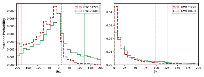
Figure 1: Posterior distributions on the spin-induced quadrupole moment parameter $\delta\kappa_{s}$, estimated from the observed gravitational wave events GW151226 Abbott et al. (2016b) and GW170608 Abbott et al. (2017b). Left and right panels correspond to two different physically motivated priors on $\delta\kappa_{s}$ parameter (symmetric and one-sided). The posteriors are obtained from the Bayesian analysis of the O1/O2 public GW data using LALInference Veitch et al. (2015). We used IMRPhenomPv2 waveform models Husa et al. (2016) for the analysis, truncated at the inspiral-to-merger transition frequency as the spin-induced deformations are not modelled in the merger and ringdown phases. The vertical dotted lines show the $90\%$ credible bounds (highest density intervals) on $\delta\kappa_{s}$.

In this work, we implement and demonstrate the method Krishnendu et al. (2017) within the framework of Bayesian inference and perform tests of binary black hole nature of the LIGO-Virgo detected binary black hole events. Our method uses binary black hole waveforms with parametrized deformations on the spin-induced quadrupole moment coefficients $\kappa$, defined as $\kappa=1+\delta\kappa$ where the parametrized deformations (labeled as $\delta\kappa$) represents the deviations from binary black hole nature. We make use of the LALInference LIGO Scientific Collaboration (2018a); Veitch et al. (2015) library to measure the parameterized deformations $\delta\kappa$ of compact binaries which can be considered as the bounds on their departures from binary black hole natures. Our method also includes estimation of Bayes factors to perform Bayesian model selection between binary black hole models and black hole mimicker models.

We perform detailed studies to demonstrate the method using simulated GW signals (injections) which include those of various masses and spins. We investigate in detail about various degeneracies in the parameter space and associated systematics in the estimated parameters, which may often restrict the applicability of this test. Finally, we apply this method on the LIGO-Virgo detected binary black holes GW151226 and GW170608 and obtain constraints on their BH natures.

I.2 Executive Summary: Constraints from GW151226 and GW170608

Here we briefly summarize the results from the tests of binary black hole nature of the observed GW signals GW151226 Abbott et al. (2016b) and GW170608 Abbott et al. (2017a). Among all the ten binary black hole events detected in O1/O2, we have restricted the analysis for these two events. This is because, with the currently available waveform models, our test is applicable only on the inspiral part of the signal and GW151226 and GW170608 are the only two inspiral dominated events.

Event	Prior	$90\%$ bounds	Bayes factor
	on $\delta\kappa_{s}$	on $\delta\kappa_{s}$	($\log\mathcal{B}^{\text{\tiny NBH}}_{\text{\tiny BH}}$)
GW151226	[-200, 200]	[-191.78, 13.45]	-0.94
	[0, 200]	$\leq$ 98.67	-2.26
GW170608	[-200, 200]	[-177.36, 122.98]	-0.15
	[0, 200]	$\leq$ 125.69	-1.15

Table 1: Summary of the tests of binary black hole nature of the real gravitational wave events GW151226 and GW170608 by measuring the spin-induced quadrupole moment parameters $\delta\kappa_{s}$. The results are shown for two different physically motivated priors on $\delta\kappa_{s}$: [-200, 200] (symmetric) and [0, 200] (one-sided) as shown in the second column. The third and fourth columns respectively show the $90\%$ credible intervals (upper bounds in case of one-sided priors) on $\delta\kappa_{s}$ and the Bayes factors between non-BH and BH models.

Figure 1 shows the bounds obtained from GW151226 Abbott et al. (2016b) (red) and GW170608 Abbott et al. (2017b) (green). We show the posterior probability distribution for $\delta\kappa_{s}$, the parametrized deformations in the $\kappa_{s}$ parameter, which is the symmetric combination of spin-induced quadrupole moment coefficients of the individual compact objects ($\kappa_{1}$ and $\kappa_{2}$), as discussed in section I.1. In the left panel, we used a generic prior on $\delta\kappa_{s}$, as uniform in [-200, 200], which leads to constraints on generic BH mimicker models which has positive or negative values for $\delta\kappa_{s}$. Under this prior assumption, we find that the deformation parameter $\delta\kappa_{s}$ is constrained to a 90% credible interval of [ -191.78, 13.45] for GW151226 and [ -177.36, 122.98] for GW170608. In the right panel, we have obtained the bounds on $\delta\kappa_{s}$ for a restricted one-sided prior of [0, 200]. Unlike the generic prior, this one-sided prior leads to constraints on specific black hole mimicker models such as boson stars for which $\delta\kappa_{s}$ is predicted to be positive always. Under this prior assumption, we obtain 90% credible upper bounds to be $\delta\kappa_{s}\leq 98.67$ for GW151226 and $\delta\kappa_{s}\leq 125.69$ for GW170608. All the bounds are listed in Table 1. In all the cases, it is noted that the BH limits ($\delta\kappa_{s}=0$) are well within the 90% credible intervals which means that the posteriors do not indicate the presence of any non-BH nature in these events. However, one may also note that the posteriors are not very sharply peaked at zero implying weaker constraints on the non-BH nature of the compact objects involved.

In addition to the bounds reported above, we performed Bayesian model selection between BH mimicker models and BH models by calculating the Bayes factor between them (defined in Sec. II.3). The estimated Bayes factors for both the events are given in Table 1. For these events, we find that the Bayes factors in the logarithmic scale are -0.94 (for GW151226) and -0.15 (for GW170608) which implies that Bayes factors do not show strong evidence in favor of any of the models (neither BH nor non-BH models). These results are in agreement with our conclusions from the posteriors discussed above. Only more sensitive measurements in the future may help us quantify this better. In section IV, we have discussed the results from gravitational wave events in more detail.

The rest of this paper is organized as follows. In Section II, we discuss the waveform model used in this study and give a brief overview of Bayesian inference for parameter estimation and model selection. Section III covers our detailed simulation studies and results, and in section IV, we present the constraints obtained from the real events GW151226 and GW170608.

II Method

II.1 The waveform model

In frequency domain, the gravitational wave signal from compact binary inspirals in the detector frame can be schematically written as,

$$\tilde{h}(f)=\mathcal{C}\,\mathcal{A}(f)\,\mbox{\large{\it{e}}}^{i{\mathit{\psi}(f)}},$$ (2)

where, $\mathit{\psi}(f)$ is the phase and $\mathcal{A}(f)$ is the amplitude of the gravitational wave signal which is given by $\sim D_{L}^{-1}\,\mathcal{M}^{5/6}\,f^{-7/6}$ where $\mathcal{M}$ is the chirp mass, which is related to individual masses $m_{1}$ and $m_{2}$ as, $\mathcal{M}$=$\frac{(m_{1}\,m_{2})^{3/5}}{(m_{1}+m_{2})^{1/5}}$, and $D_{L}$ is the luminosity distance to the source. The factor $\mathcal{C}$ carries the antenna response of the interferometers as a function of the source location and orientation parameters.

The orbital evolution of the inspiralling binary is largely encoded in the phasing formula and appears in terms of the masses and spins of the binary . Due to the recent developments in the post-Newtonian modeling of compact binaries Blanchet (2014), the phasing formula for the inspiralling binary has been computed accurately up to 3.5PN order Marsat et al. (2013); Bohé et al. (2013a, b); Marsat et al. (2014); Bohé et al. (2015); Marsat (2015); Arun et al. (2009); Kidder (1995); Will and Wiseman (1996); Buonanno et al. (2013); Blanchet (2014); Mishra et al. (2016); Buonanno and Damour (1999); Nagar et al. (2018); Pan et al. (2014).

This phasing formula accounts for the higher-order spin corrections such as spin-orbit interactions (at 1.5PN, 2PN, 3PN and 3.5PN orders) and spin-spin interactions (at 2PN and 3PN orders). Spin-induced quadrupole moment coefficient given in Eq. (1) first appears at the 2PN order and its first post-Newtonian correction appears at the 3PN order Marsat et al. (2013); Bohé et al. (2013a, b); Marsat et al. (2014); Bohé et al. (2015); Marsat (2015).

Since the spin-induced quadrupole moment parameter is unity for Kerr BHs, the waveforms which are particularly developed for binary black hole systems a priori assume the value unity. However, for this study, since our interest is in those binary systems for which $\kappa$ departs from unity, we re-write Eq. (1) in the following form,

$$Q=-(1+\delta\kappa)\,\chi^{2}\,m^{3},$$ (3)

where $\delta\kappa$ is the parametrized departure of $\kappa$ from unity. Hence $\delta\kappa=0$ is the BH limit and non-zero $\delta\kappa$ corresponds to non-BH objects. Our proposal is to independently measure $\delta\kappa$ and use the measurement to put possible constraints on the allowed parameter space of BH mimicker models from observed gravitational wave events.

For this study, we use the IMRPhenomPv2 Hannam et al. (2014) waveform approximant which is available in LSC Algorithm Library, by incorporating into it, the parametrized deformations shown in Eq. (3). IMRPhenomPv2 is a frequency domain inspiral-merger-ringdown waveform model whose inspiral part of the phasing agrees with the PN phasing and the merger-ringdown parts are obtained by calibrating to the numerical-relativity waveforms Taracchini et al. (2014); Buonanno and Damour (2000); Hannam et al. (2014); Buonanno and Damour (1999); Ajith et al. (2011). These numerical-relativity waveforms have been computed by assuming binary black hole nature (ie, $\delta\kappa_{s}=0$) by default. Therefore the merger and ringdown phases of the IMRPhenomPv2 do not account for the $\kappa$ effects hence the analytical parametrization described in Eq. (3) is not expected to be valid once the binary enters into the merger regime of the evolution. To avoid any systematic biases due to this, we truncate our analysis at the inspiral-to-merger transition frequency of the IMRPhenomPv2 defined by $f_{\rm{upper}}=0.018/M$, where $M$ is the total mass of the system Husa et al. (2016). As investigated in Ref. Ghosh et al. (2018), we expect negligible amount of spectral leakage effects due to this sharp cut-off.

II.2 Choice of test parameters

In the most general case, each compact object in the binary can have independent spin-induced quadrupole moments $\kappa_{1}$ and $\kappa_{2}$ which are different from the Kerr value of unity. Hence we can parametrize a potential deviation of the BH nature by introducing two independent deformation parameters $\delta\kappa_{1}$ and $\delta\kappa_{2}$ given by $\kappa_{1,2}=1+\delta\kappa_{1,2}$. Due to the strong degeneracy between $\delta\kappa_{1,2}$ in the gravitational waveform, simultaneous measurement of the two would yield very weak constraints Krishnendu et al. (2017, 2018).

Hence one may resort to an alternative approach where one of the linear combinations of the $\delta\kappa_{1,2}$ parameters is estimated from the data. Following Krishnendu et al. (2017), we consider the symmetric combination $\delta\kappa_{s}=\frac{1}{2}(\delta\kappa_{1}+\delta\kappa_{2})$ as the parameter which captures the deviation from binary black hole nature and estimates the associated error bars when the anti-symmetric combination is zero ($\delta\kappa_{1}=\delta\kappa_{2}$). Though restrictive, this does not weaken the proposed null test because a break down of this assumption is also likely to lead to a shift of the peak of the posterior of $\delta\kappa_{s}$ away from zero which is what we look for as evidence for the presence of black hole mimickers.

II.3 Overview of Bayesian inference

We provide a brief review of Bayesian inference for gravitational wave parameter estimation and model selection keeping the present context of testing the binary black hole nature in mind. The subject has been well described in literature Veitch et al. (2015); Veitch and Vecchio (2010).

Given the data d, which contains the signal and the noise, if $\mathcal{H}$ is our hypothesis (or model) about the signal, then following Bayes’ theorem, the posterior probability of the signal parameters $\bar{\theta}$ can be written as,

$$P(\bar{\theta}|\mathcal{H},d)=\frac{P(\bar{\theta}|\mathcal{H})\,P(d|\mathcal{H},\bar{\theta})}{P(d|\mathcal{H})},$$ (4)

where, $P(\bar{\theta}|\mathcal{H})$ is the prior probability and $P(d\,|\bar{\theta},\mathcal{H})$ is the likelihood function. For a Gaussian wide-sense stationary noise, the likelihood function can be expressed as,

$$P(d|\mathcal{H},\,\bar{\theta})\propto\exp{\left[-\frac{(\tilde{{d}}-\tilde{{h}}|\tilde{{d}}-\tilde{{h}})}{2}\right]},$$ (5)

where, $\tilde{{d}}$ and $\tilde{{h}}$ are respectively the data and model waveform in frequency domain. The noise weighted inner product $(.|.)$ appearing in the exponent is defined as

$$(x|y)=4\Re\int_{f_{\text{lower}}}^{f_{\text{upper}}}\frac{x(f)^{*}y(f)}{{S_{n}}(f)}df$$ (6)

where the ^∗ indicates complex conjugate and ${S_{n}}(f)$ is the one-sided power spectral density (PSD) of the noise. The lower limit of integration $f_{\text{lower}}$ is the seismic cut-off frequency and the upper limit $f_{\text{upper}}$ is the inspiral-to-merger transition frequency discussed in section II.1. $P(d|\mathcal{H})$ in Eq. (4) is the Bayesian evidence for the model $\mathcal{H}$, denoted by $\mathcal{Z}$, which is obtained as the likelihood marginalized over the prior volume,

$$\mathcal{Z}=P(d|\mathcal{H})=\int P(\bar{\theta}|\mathcal{H})\,P(d|\bar{\theta},\mathcal{H})d\bar{\theta},$$ (7)

where the integration is over the entire prior volume of the multi-dimensional parameter space. Evidence quantifies how much the data $d$ is in favor of the model $\mathcal{H}$ within the prior domain.

To test the binary black hole nature of the compact binaries, we define the following two models:

1. The binary black hole model $\mathcal{H}_{\text{\tiny BH}}$ which reads as “The source of the gravitational wave signal is binary black holes in general relativity”. For this model, the waveform assumes $\kappa_{s}$ to be unity (or $\delta\kappa_{s}=0$) and the set of parameters defining this model (i.e., binary black hole parameters) is denoted as $\bar{\theta}_{\text{\tiny BH}}$.

2. The non-BH model $\mathcal{H}_{\text{\tiny NBH}}$ which reads as “ The source of the gravitational wave signal is a binary of non-BH compact objects aka BH mimickers”. The waveform for this model allows $\kappa_{s}$ to deviate from unity. Therefore we use $\delta\kappa_{s}$ as a free parameter and the set of parameters defining this model is given as $\bar{\theta}_{\text{\tiny NBH}}=\{\bar{\theta}_{\text{\tiny BH}},\delta\kappa_{s}\}$.

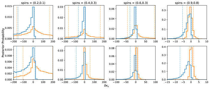
Figure 2: Posterior distributions on $\delta\kappa_{s}$ for a binary systems with total mass 15$M_{\odot}$ and mass ratio 1 (top row) and 2 (bottom row) for different spin magnitudes of (0.2, 0.1), (0.4, 0.3), ( 0.6, 0.3) and ( 0.9, 0.8) from left to right in each row. Binaries are assumed to be optimally oriented at a luminosity distance of 400 Mpc. Different colours represent different injected spin orientations: both spins aligned to the orbital angular momentum (light blue) and both spins anti-aligned to the orbital angular momentum (orange).

The one-dimensional posterior for $\delta\kappa_{s}$ parameter can be obtained by marginalizing the multi-dimensional posterior over the other parameters, i.e.,

$$P(\delta\kappa_{s}|\mathcal{H}_{\text{\tiny NBH}},\,d)=\int P\left(\{\bar{\theta}_{\text{\tiny BH}},\delta\kappa_{s}\}|\mathcal{H}_{\text{\tiny NBH}},d\right)\,d\bar{\theta}_{\text{\tiny BH}},$$ (8)

and the 90% credible intervals on $\delta\kappa_{s}$ are obtained as the shortest interval $(\delta\kappa_{s}^{l},\delta\kappa_{s}^{r})$ which contains 90% of the posterior probability distribution, i.e.,

$$\int_{\delta\kappa_{s}^{l}}^{\delta\kappa_{s}^{r}}P(\delta\kappa_{s}\,|\mathcal{H}_{\text{\tiny NBH}},\,d)\,d\delta\kappa_{s}\sim 0.9.$$ (9)

To perform model selection between the BH and non-BH models, we compute the Bayes factor between $\mathcal{H}_{\text{\tiny NBH}}$ and $\mathcal{H}_{\text{\tiny BH}}$ as follows,

$$\mathcal{B}^{\text{\tiny NBH}}_{\text{\tiny BH}}=\frac{\mathcal{Z}_{\text{\tiny NBH}}}{\mathcal{Z}_{\text{\tiny BH}}},$$ (10)

which quantifies how well the data favors the BH mimicker hypothesis $\mathcal{H}_{\text{\tiny NBH}}$ over the BH hypothesis $\mathcal{H}_{\text{\tiny BH}}$. When there is no prior preference for one model over the other, then Bayes factor is same as the odds ratio between the two models (Odds ratio is defined as the ratio of posterior probabilities of the two models i.e., $P(\mathcal{H}_{\text{\tiny NBH}}|d)/P(\mathcal{H}_{\text{\tiny BH}}|d)$). Following definition of evidence in Eq. (7), the Bayes factor in Eq. (10) can be written as,

$$\mathcal{B}^{\text{\tiny NBH}}_{\text{\tiny BH}}=\frac{\int P(\bar{\theta}_{\text{\tiny NBH}}|\mathcal{H}_{\text{\tiny NBH}})\,P(d|\bar{\theta}_{\text{\tiny NBH}},\mathcal{H}_{\text{\tiny NBH}})d\bar{\theta}_{\text{\tiny BH}}\,d\delta\kappa_{s}}{\int P(\bar{\theta}_{\text{\tiny BH}}|\mathcal{H}_{\text{\tiny BH}})\,P(d|\bar{\theta}_{\text{\tiny BH}},\mathcal{H}_{\text{\tiny BH}})\,d\bar{\theta}_{\text{\tiny BH}}}.$$ (11)

For both parameter estimation as well as model selection studies in this paper, we use LALInference Veitch et al. (2015) which is a Bayesian inference package available in the LSC Algorithm Library LIGO Scientific Collaboration (2018a); Veitch et al. (2015). LALInference makes use of stochastic sampling algorithms such as Nested Sampling Skilling (2006), Markov Chain Monte Carlo (MCMC) sampling Feroz and Hobson (2008); Feroz et al. (2009, 2013) etc. and we use Nested Sampling algorithm for the analysis in this study.

III Studies using simulated data and results

In this section, we perform detailed studies using simulated data to assess the efficiency of the proposed method to distinguish between binary black holes and binaries comprising of black hole mimickers. The aim is primarily to quantify the bounds on the $\delta\kappa_{s}$ parameter as a function of the source parameters of the expected gravitational wave signal. We also present the Bayes factors between black hole mimickers and black hole models as a function of $\delta\kappa_{s}$.

III.1 Details of simulations

Masses: We choose binary systems with the total mass $M=15M_{\odot}$ in the detector frame and mass ratios $q=1$ and $q=2$ as representative cases. The masses are chosen such that they ensure the signals have a significant amount of inspiral in the detector band as the parametrization we employ is in the inspiral part of the waveform.

Spins: Four combinations of component spins (dimensionless spin magnitudes) are used: (0.2, 0.1), (0.4, 0.3), (0.6, 0.3) and (0.9, 0.8) which represent low, moderate, and high spins, respectively here the heavier BH in the binary always assumed to be highly spinning compared to the lower mass BH. Each component spin can be either aligned or anti-aligned with respect to the orbital angular momentum vector. Therefore, for each binary we consider four possible spin configurations: both are aligned, the heavier BH spin is aligned but the lighter BH spin is anti-aligned, the heavier BH spin is anti-aligned but the lighter BH spin is aligned and both BH spins are anti-aligned.

$\delta\kappa_{s}$ parameter: Binary black hole injections are generated with $\delta\kappa_{s}$=0 while non-BH injections are generated by choosing $\delta\kappa_{s}$ in the range [-40, 40]. The non-BH injections are used to compute the Bayes factors between the non-BH and BH hypotheses.

Extrinsic parameters: We choose a fixed distance of 400 Mpc for all the systems which is broadly motivated by the typical distances of several binary black hole mergers during the first two observing runs of Advanced LIGO and Advanced Virgo. For all the systems above, the sky-location and orientation are chosen in such a way that they are optimally oriented and located for the detector network under consideration. Both sky-location and orientation of the source can affect our estimates of $\delta\kappa_{s}$ only through the signal-to-noise ratio.

Prior choices: We use prior on $\delta\kappa_{s}$ to be uniform in [-200, 200]. This range includes the spin-induced quadrupole moment values predicted for various binary black hole mimicker models Ryan (1997); Uchikata and Yoshida (2016). Priors on the dimensionless spin parameters (component spins) are chosen such that their magnitudes are uniform in [0, 1] and their directions are isotropically distributed. Component mass priors are uniform in [4, 100]$M_{\odot}$. Further, all the injections are non-precessing (i.e., aligned or anti-aligned spins) whereas the recovery waveform models account for precession effects.

Network configuration: Throughout our studies, we consider a three-detector network (HLV) which includes two advanced LIGO detectors at Hanford (H) and Livingston (L) LIGO Scientific Collaboration (2018b); Harry (2010); LIGO Scientific Collaboration (2009a) and advanced Virgo detector (V) Acernese and et.al. (2006); Acernese et al. (2015), assuming both LIGO and Virgo at their design sensitivities given by references LIGO Scientific Collaboration (2018c) and LIGO Scientific Collaboration (2018d); Acernese and et.al. (2006), respectively.

Zero-noise injections: Injections are generated using the lalsim-inspiral library available in the LSC Algorithm Library LIGO Scientific Collaboration (2018a) with IMRPhenomPv2 as the waveform approximant. For all the injections, we assume noise realizations to be zero (zero-noise injections) in order to avoid biases in the parameter estimates introduced by a particular noise realization. Results from a zero-noise realization is equivalent to results averaged over many realizations of zero-mean random noise. A noise realization is not to be confused with the noise PSD $S_{n}(f)$ which appears in the likelihood integral (see Eq. (6)) which is always used while computing the relevant quantities.

Other details: For the current analysis, we use a sensitive lower cut-off frequency of $f_{\text{lower}}=$20Hz for all three detectors. The upper cut-off frequency $f_{\text{upper}}$ of the integral in Eq. (6) is chosen as the inspiral-to-merger transition frequency of the IMRPhenomPv2 waveform which is related to the total mass of the system through the relation $M\,f_{\rm{upper}}=0.018$ Husa et al. (2016), as described earlier. With all these criterions applied, our test injections have the three-detector (LHV) network SNR ranging between $\sim$40-45, where the slight variations are caused by the spins.

The neglect of the merger and ringdown parts of the waveform will lead to deterioration in the overall parameter estimation. As mentioned before, this is why we choose the injections with total mass of $M=15M_{\odot}$ so that the SNR contribution from the merger and ringdown is as low as $\sim 3\%$ of the total SNR, assuming zero spins. For GW151226 and GW170608 on which we have applied the test in this work, the SNR contributions from the merger and ringdown are $\sim 7\%$ and $\sim 5\%$ respectively. However, we would like to stress that the neglect of merger and ringdown in our case is due to the unavailability of a physical model for spin-induced multipole moments beyond the inspiral. In future, with better analytical understanding of the dynamics of the remnant black holes, situation may change (see, for example, Gupta et al. (2018) for a recent work along this direction).

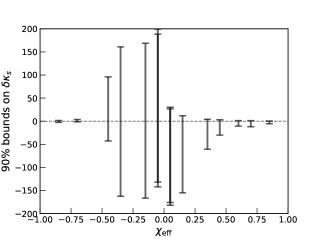
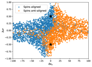
Figure 3: Left: The $90\%$ bounds on the spin-induced quadrupole moment parameter $(\delta\kappa_{s})$ given in Eq. (9) as a function of the injected valuees of effective spin parameter (see Eq. (12)). All the injections are compact binary inspirals with fixed total mass of $15M_{\odot}$ while varying the mass ratio, spin magnitudes and orientations which results in different values of effective spin parameter. Right: Figure showing the degenerate regions in the non-BH parameter space ($\delta\kappa_{s}-\chi_{\text{eff}}$) for binary black hole injections with two different spin orientations aligned (0.6, 0.3) and anti-aligned (-0.6, -0.3). The light blue and orange represent aligned and anti-aligned cases respectively and the injected parameters are marked by black stars. The scattered points show the region at which the non-BH waveform has a very high overlap (${\cal O}>0.995$) with the BH injection(s) (See Eq. (13)).

III.2 Bounds on $\delta\kappa_{s}$ parameter

Fig. 2 shows the posterior probability distributions of $\delta\kappa_{s}$ parameter obtained from the various simulations. The first row corresponds to component masses (7.5, 7.5)$M_{\odot}$ (mass ratio = 1) and the second row corresponds to component masses (10, 5)$M_{\odot}$ (mass ratio = 2). In each row, the four different columns correspond to four spin magnitudes (0.2, 0.1), ( 0.4, 0.3), (0.6, 0.3) and (0.9, 0.8) from left to right. The different colors represent different injected spin orientations: both the spins aligned (light blue) and both spins anti-aligned (orange) to the orbital angular momentum axis. The dashed vertical lines are the 90% credible bounds following the respective colors of the histograms. Recall that the bounds are estimated as the highest density intervals of the posteriors as defined in Eq. (9).

It is evident from Fig. 2 that the bounds on $\delta\kappa_{s}$ are stronger when the spin magnitudes are larger (see the panels from left to right together with their narrowing axis range). This is expected because, for larger spin magnitudes, the waveform has stronger signatures of spin-induced quadrupole moments (see Eq. (3)) which in turn improves the measurement.

Though all the posteriors in Fig. 2 peak at their injected values ($\delta\kappa_{s}=0$), we notice that there is skewness in all the posteriors about their injected values. This skewness gets mirror-reflected when the spin orientation is reversed. In other words, comparing the light blue and orange histograms in each panel, one notices that the longer tail for light blue is towards left-hand side while for orange, it is towards the right-hand side. This indicates that our ability to constrain the non-BH nature is different for aligned and anti-aligned spin orientations. For aligned cases, the type of non-BH nature with $\delta\kappa_{s}>0$ (such as binaries of boson stars) can be better constrained than the type of non-BH nature with $\delta\kappa_{s}<0$ (such as binaries of gravastars). On the other hand, for anti-aligned cases, it is vice versa. We investigate these features in detail below.

III.2.1 Role of effective spin parameter

We find that the effective spin parameter $\chi_{\text{eff}}$ plays a major role in the features observed in the posteriors discussed above. Effective spin parameter defined as

$$\chi_{\rm{eff}}=\frac{m_{1}\,\chi_{1z}+m_{2}\,\chi_{2z}}{(m_{1}+m_{2})},$$ (12)

is a combination of component masses $m_{1}$, $m_{2}$ and component spins $\chi_{1z}$, $\chi_{2z}$ and appears as the leading order spin dependence in the inspiral PN waveform Ajith et al. (2011). In Fig. 3 (left panel), we have shown the bounds on $\delta\kappa_{s}$ parameter as a function of their injected $\chi_{\text{eff}}$ values where the vertical bars correspond to the 90% credible intervals of the $\delta\kappa_{s}$ parameter. The larger the magnitude of $\chi_{\rm eff}$, the tighter the bounds on $\delta\kappa_{s}$. For systems with small magnitudes of $\chi_{\rm eff}$ (for example, $\chi_{\rm eff}<0.3$), the $\delta\kappa_{s}$ parameter is almost unconstrained. Further, when $\chi_{\text{eff}}$ is large and positive, the region with $\delta\kappa_{s}>0$ is better constrained, whereas when the $\chi_{\text{eff}}$ is large and negative, the region with $\delta\kappa_{s}<0$ is better constrained.

The dependence of $\delta\kappa_{s}$ posteriors on $\chi_{\text{eff}}$ discussed above holds true despite the fact that the systems considered for this plot include those with various component masses and spins. In fact, it is difficult to disentangle the individual effects of the component masses and spins due to the degeneracy between spins and mass ratio parameters Baird et al. (2013). However, $\chi_{\rm eff}$ captures the combined effects of all these parameters on the $\delta\kappa_{s}$ posteriors and hence is the most important single parameter which describes our ability to constrain $\delta\kappa_{s}$ parameter for any given system.

We further investigate the skewness of the posteriors in detail and show that they are primarily caused by the waveform degeneracies between $\delta\kappa_{s}$ and $\chi_{\text{eff}}$ parameters. To demonstrate this, we first define the overlap function $\mathcal{O}$ between a binary black hole injection $\tilde{h}^{\rm{BH}}$ and a non-BH template $\tilde{h}^{\rm{NBH}}$ as,

$$\mathcal{O}=\frac{\left(\tilde{h}^{\text{\tiny BH}}|\tilde{h}^{\text{\tiny NBH}}\right)}{\sqrt{\left(\tilde{h}^{\text{\tiny BH}}|\tilde{h}^{\text{\tiny BH}}\right)\left(\tilde{h}^{\text{\tiny NBH}}|\tilde{h}^{\text{\tiny NBH}}\right)}}$$ (13)

where $(.|.)$ is the noise weighted inner product defined in Eq. (6) and both $\tilde{h}^{\text{\tiny BH}}$ and $\tilde{h}^{\text{\tiny NBH}}$ are in frequency domain. Overlap quantifies how similar are the two signals $\tilde{h}^{\text{\tiny BH}}$ and $\tilde{h}^{\text{\tiny NBH}}$ and its value is maximum ($\mathcal{O}=1$) when $\tilde{h}^{\text{\tiny BH}}=\tilde{h}^{\text{\tiny NBH}}$.

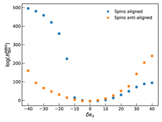
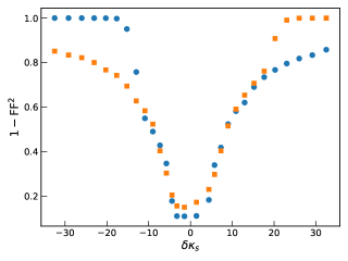
Figure 4: Left: Demonstration of Bayes factor between non-BH and BH models for different non-BH injections. The x-axis shows the injected value of $\delta\kappa_{s}$ and y-axis shows the log of Bayes factors. All the injections are of component masses $(10+5)M_{\odot}$ and fixed spin magnitudes $(0.6,0.3)$ while the light blue and orange markers correspond to aligned and anti-aligned spin orientations respectively. Right: Complementary analysis done using fitting factors motivated by Vallisneri (2012). For each non-BH injection with values of $\delta\kappa_{s}$ as given on x-axis, the fitting factor $\rm{FF}$ was computed w.r.t the BH waveforms by maximizing the overlap over the BH parameter space. Here the maximization is done on a restricted BH parameter space with $\chi_{\text{eff}}$ being the only free parameter, with the remaining parameters fixed to their injected values. The quantity on y-axis is $1-\rm{FF}^{2}$ which explicitly appears in the approximate scheme of Vallisneri (2012) (See Eq. (15))

We have taken two binary black hole injections with both of them having identical component masses $(10,5)M_{\odot}$ but different spin orientations (0.6, 0.3) and (-0.6, -0.3) whose $\chi_{\text{eff}}$ values are $0.5$ and $-0.5$ respectively. The templates $\tilde{h}^{\rm{NBH}}$ are uniformly distributed in the non-BH parameter space with component spins ranging in [-1, 1] and $\delta\kappa_{s}$ ranging between [-100, 100]. The masses of the templates are kept fixed at their injection values which will be justified later with the results.

We show the results of this overlap calculation in the right panel of Fig. 3. Templates having very high overlaps with the injections ($\mathcal{O}>0.995$) are shown as scattered plots in the $\delta\kappa_{s}-\chi_{\text{eff}}$ plane (light blue for aligned-spin injection and orange for anti-aligned spin injection). The injected parameters are marked with stars (black color). For the aligned spin case (light blue), there are more scattered points on the left half ($\delta\kappa_{s}<0$) compared to the right half ($\delta\kappa_{s}>0$). This indicates that the left half is more degenerate and hence less distinguishable from the injected binary black hole signal, compared to the right half. This is exactly the feature observed in the posteriors as well as the bar plot (Fig. 2 and Fig. 3 left) that for systems with aligned spins (or $\chi_{\text{eff}}>0$), the positive side of the $\delta\kappa_{s}$ posterior is better constrained than the negative side. A similar explanation holds for the anti-aligned spin case as well with all the features turned exactly opposite.

The fact that the masses of the templates are fixed to the injected values might be considered as ignoring some of the other potential degeneracies which are present. However, ignoring the role of such degeneracies can be justified since we have shown above that the $\delta\kappa_{s}-\chi_{\text{eff}}$ degeneracies could solely explain the features of the posteriors. In other words, the overlap study with masses fixed to the injections helps underline that it is the $\delta\kappa_{s}-\chi_{\text{eff}}$ degeneracy which is primarily responsible for the features of the posteriors.

III.3 Model selection between BH and non-BH models

In this section, we discuss the model selection studies between non-BH and BH models by obtaining Bayes factors between them. We estimate the Bayes factors $\mathcal{B}^{\text{\tiny NBH}}_{\text{\tiny BH}}$ (see Eq. (11)) using LALInference for a set of non-BH injections whose $\delta\kappa_{s}$ varies in the range [-40, 40]. All the injections are of fixed component masses (10, 5)$M_{\odot}$ while the analysis is repeated with two spin choices for the injections: (0.6, 0.3) and (-0.6, -0.3), which as followed in the previous section, represents the aligned and anti-aligned orientations respectively.

The results are shown in the left panel of Fig. 4 where the log of the Bayes factors ($\log\mathcal{B}^{\text{\tiny NBH}}_{\text{\tiny BH}}$) are plotted as a function of the injected $\delta\kappa_{s}$ values. The light blue and orange colors correspond to aligned and anti-aligned spins respectively. As one would expect, when the magnitude of the injected $\delta\kappa_{s}$ increases, the Bayes factor increases which mean that they can be better distinguished from binary black hole models. We notice that the way Bayes factor increases with $\delta\kappa_{s}$ is different for aligned and anti-aligned cases. For example, among all the injections with $\delta\kappa_{s}>0$ (such as binaries of boson stars), Bayes factors are larger for those whose spins are anti-aligned (or negative $\chi_{\text{eff}}$) compared to those whose spins are aligned (or positive $\chi_{\text{eff}}$). The reverse is true for the injections with $\delta\kappa_{s}<0$ (such as binaries of gravastars).

The features discussed above can have possible consequences on the identification of BH mimicker populations. For example, among the population of boson star binaries, our ability to distinguish them from binary black holes will be inclined towards those with anti-aligned spins. As a result, the population which we identify as binary boson stars will have more sources with anti-aligned spins (or negative $\chi_{\text{eff}}$). Similarly, the population which we identify as binary gravastars will have more sources with aligned spins (or positive $\chi_{\text{eff}}$).

III.3.1 Further investigations using Fitting Factor

In order to investigate various features in the Bayes factor plot (Fig. 4, left panel), we perform a study using fitting factor to complement the Bayesian analysis. The fitting factor of a non-BH waveform $\tilde{h}^{\text{\tiny NBH}}$, with a BH waveform model $\tilde{h}^{\text{\tiny BH}}$ is given by,

$$\rm{FF}(\bar{\theta}_{\text{\tiny NBH}})=\max_{\bar{\theta}_{\text{\tiny BH}}}\left(\frac{\left(\tilde{h}^{\text{\tiny NBH}}|\tilde{h}^{\text{\tiny BH}}(\bar{\theta}_{\text{\tiny BH}})\right)}{\sqrt{\left(\tilde{h}^{\text{\tiny NBH}}|\tilde{h}^{\text{\tiny NBH}}\right)\left(\tilde{h}^{\text{\tiny BH}}(\bar{\theta}_{\text{\tiny BH}})|\tilde{h}^{\text{\tiny BH}}(\bar{\theta}_{\text{\tiny BH}})\right)}}\right)$$ (14)

where $\tilde{h}^{\text{\tiny NBH}}$ is evaluated at a given point $\bar{\theta}_{\text{\tiny NBH}}$ in the non-BH parameter space and $\bar{\theta}_{\text{\tiny BH}}$ is any arbitrary point in the BH parameter space over which the maximisation is carried out. One can see from Eq. (14) that $\rm{FF}(\bar{\theta}_{\text{\tiny NBH}})$ is equal to the overlap, defined in Eq. (13), maximised over the BH parameter space. Qualitatively, $\rm{FF}(\bar{\theta}_{\text{\tiny NBH}})$ is regarded as a measure of how well the BH waveform model $\tilde{h}^{\text{\tiny BH}}$ can mimic the given non-BH signal $\tilde{h}^{\text{\tiny NBH}}(\bar{\theta}_{\text{\tiny NBH}})$. In other words, $\rm{FF}(\bar{\theta}_{\text{\tiny NBH}})$ describes how well the non-BH corrections contained in $\tilde{h}^{\text{\tiny NBH}}(\bar{\theta}_{\text{\tiny NBH}})$ can be re-absorbed into the BH waveform $\tilde{h}^{\text{\tiny BH}}(\bar{\theta}_{\text{\tiny BH}})$, by varying $\bar{\theta}_{\text{\tiny BH}}$ within its allowed range.

As discussed before, the Bayes factor $\mathcal{B}^{\text{\tiny NBH}}_{\text{\tiny BH}}$ for a given signal is high when the signal has a non-BH component of the form that can not be re-absorbed into the BH waveform. Broadly this implies that a high Bayes factor is closely related to a low fitting factor. Cornish et al. Cornish et al. (2011) and Vallisneri et al. Vallisneri (2012) showed an approximate scheme to relate the Bayes factor and fitting factor which, for our context (considering only the dominant term in the expression) would read as,

$$\log\mathcal{B}^{\text{\tiny NBH}}_{\text{\tiny BH}}\propto\rho^{2}\times\left(1-\rm{FF}(\bar{\theta}_{\text{\tiny NBH}})^{2}\right)$$ (15)

where $\rho$ is the signal-to-noise ratio. In a later work, Del Pozzo et al. Del Pozzo et al. (2014) explored this in more detail using numerical simulations and extended its validity regimes by introducing additional correction terms.

In this exercise, we consider a set of non-BH injections similar to the ones considered in the Bayes factor studies above. For all the injections, we compute $\rm{FF}(\bar{\theta}_{\text{\tiny NBH}})$ using Eq. (14) for a binary system of masses (10, 5)$M_{\odot}$. Note that in our case the BH parameter space ($\bar{\theta}_{\text{\tiny BH}}$) over which the maximization is done has only one free parameter which is the effective spin $\chi_{\text{eff}}$, while all other parameters are fixed to their injected values as our goal is to understand the ability of $\chi_{\text{eff}}$ to mimic non-BH signals.

The results are shown in the right panel of Fig. 4 where $1-\rm{FF}(\bar{\theta}_{\text{\tiny NBH}})^{2}$ (which explicitly appears in Eq. i(15)) is plotted as a function of the injected $\delta\kappa_{s}$. We find similar features as seen in the Bayes factor plot (left panel). For example, for non-BH injections with $\delta\kappa_{s}>0$, the value of $(1-\rm{FF}^{2})$ is higher for anti-aligned cases (or negative $\chi_{\text{eff}}$ cases) while it is the opposite for those injections which have $\delta\kappa_{s}<0$. That means the results independently obtained from the Bayes factor and the fitting factor analyses are complementary to each other. We emphasize again that this agreement holds despite restricting the BH parameter space to just one parameter, $\chi_{\text{eff}}$.

Thus, the fitting factor analysis further underscores the key role played by the $\chi_{\text{eff}}$-$\delta\kappa_{s}$ degeneracy in distinguishing non-BH binaries from BH binaries.

Notice that when the non-BH signals are mimicked by the BH waveforms, it happens at the cost of offsets in the estimated BH parameters from their true values. In realistic cases, this will result in systematic biases in the estimated BH parameters, if BH waveforms are used for the analysis while the true signal was of a non-BH binary. It is worth mentioning the two contexts in which this can happen. 1) if one presumes the signal to be of BH nature and hence ignore the possibility of any potential non-BH nature. 2) one does not assume BH nature a priori, however, given the SNR of the signal, the non-BH component in the signal is mild enough to be reabsorbed into the BH waveform by varying the parameters. Though both the biases are fundamental in nature Yunes and Pretorius (2009); Cornish et al. (2011), the former is also the result of our prior assumption while the latter is the result of our waveform models being insufficient to account for the underlying non-BH effects or/and the non-BH effects being buried in noise. In a follow-up work, these effects will be investigated in detail.

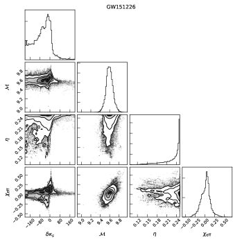
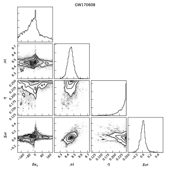
Figure 5: The corner plots of $\delta\kappa_{s}$, chirp mass ($\mathcal{M}$), symmetric mass ratio ($\eta$) and $\chi_{\rm{eff}}$ from GW151226 Abbott et al. (2016b) and GW170608 Abbott et al. (2017b) with symmetric priors on $\delta\kappa_{s}$.

IV Testing the binary black hole nature of GW151226 and GW170608

As reported in Abbott et al. (2018), the first two observation runs (O1/O2) of Advanced LIGO and Advanced Virgo have identified ten gravitational wave signals which are consistent with binary black hole waveforms. In this section, we apply the proposed spin-induced quadrupole moment test on some of the observed events and ask how consistent they are to the binary black hole hypothesis. As discussed before, at present, our test is based on a parametrization of the inspiral part of the waveform. Therefore, we restrict the study to the two inspiral-dominated signals GW151226 Abbott et al. (2016b) and GW170608 Abbott et al. (2017b), where the inspiral only signal to noise ratio is at least $\sim 10$. The estimated (median) detector frame total mass of GW151226 and GW170608 are $23.55M_{\odot}$ and $19.89M_{\odot}$ LIGO Scientific Collaboration (2009b) and the corresponding inspiral-to-merger transition frequencies are $155.12$Hz and $184.55$Hz respectively. We use these as the upper cut-off frequencies ($f_{\text{upper}}$) of the analyses along with IMRPhenomPv2 as the waveform approximant.

The main results are shown in Fig. 1 where the posteriors on $\delta\kappa_{s}$ parameter are discussed (as we summarized in section I.2). We consider two different priors on $\delta\kappa_{s}$: a symmetric prior $[-200,200]$ (left panel) and a one-sided prior $[0,200]$ (right panel). The symmetric prior [-200, 200] represents a most generic test which accounts for BH mimicker models including those of both oblate ($\delta\kappa_{s}>0$) and prolate ($\delta\kappa_{s}<0$) spin-induced deformations. The one-sided prior [0, 200] is a restricted case which accounts only for oblate spin-induced deformations. In other words, the symmetric prior leads to generic constraints on BH mimicker models including boson stars, gravastars etc. whereas the one-sided prior is motivated by specific models such as boson star models for which $\delta\kappa_{s}$ is always positive and hence meant to provide specific constraints on such models. The prior is restricted to $|\delta\kappa_{s}|\leq 200$ because the parametrized waveforms we construct are found not to be well-behaved beyond this range and hence cannot meaningfully represent the corresponding physics. The 90% credible intervals (highest density intervals) on $\delta\kappa_{s}$ are given in Table 1. For all the cases, it is found that the 90% credible intervals or the upper bounds (in case of one-sided prior) are consistent with $\delta\kappa_{s}$ being equal to zero and hence consistent with GW151226 and GW170608 being binary black holes.

Detailed corner plots are presented in Fig. 5 which will help us to gain further insights about the underlying degeneracies and correlations. As we discussed earlier, the $\delta\kappa_{s}$ parameter is found to be highly degenerate with $\chi_{\text{eff}}$. Again, we note that the posteriors of $\delta\kappa_{s}$ are asymmetric about their most probable values and both the events have got more posterior support for negative values of $\delta\kappa_{s}$ than positive values. We recall from Fig. 2 and 3 that the similar posterior features were observed for cases in which positive values of $\chi_{\text{eff}}$ were injected. As seen in the corner plots, the estimated (median) $\chi_{\text{eff}}$ values are positive for both these events and hence the results from these two events are completely consistent with our findings from simulation studies. It is also found that the $\delta\kappa_{s}$ posteriors are railing against the prior boundaries for both the events. This may improve in future if there are events which have larger spins or lower masses, similar to the ones considered in the simulations earlier.

We also performed Bayes factor studies on both the events whose results are also shown in Table 1. With the symmetric and the one-sided priors on $\delta\kappa_{s}$, we computed Bayes factors ($\mathcal{B}^{\text{\tiny NBH}}_{\text{\tiny BH}}$) between the non-BH and BH models ($\mathcal{H}_{\text{\tiny NBH}}$ and $\mathcal{H}_{\text{\tiny BH}}$ respectively). We find that the log of the Bayes factors ($\log\mathcal{B}^{\text{\tiny NBH}}_{\text{\tiny BH}}$) are in the range $-2.3<\log\mathcal{B}^{\text{\tiny NBH}}_{\text{\tiny BH}}<0$ for all the cases. These values are too small to be considered as evidence for favoring or rejecting any of the models which are tested. The slightly negative values obtained in all the cases may be interpreted as weak evidence in favor of BH models over non-BH models. We notice that these features are consistent with those observed in the posteriors in Fig. 1 that the posteriors are spread over a wider range of values of $\delta\kappa_{s}$ with significant weights over non-BH (i.e. non-zero) values.

V Conclusions and Outlook

In this work, we have developed a Bayesian framework to test the binary black hole nature of gravitational wave signals using the measurements of spin-induced quadrupole moment parameters of the compact binaries as proposed in Ref. Krishnendu et al. (2017). We carried out detailed studies using simulated gravitational wave signals to test the applicability of our method. The waveform models which are used for this test currently includes spin-induced deformation terms only in the inspiral part and hence its applicability is limited to the inspiral regime.

We applied the method on the two inspiral-dominated events from O1/O2, GW151226 and GW170608, and obtained bounds on their binary blackhole natures. These are the first constraints on the black hole nature of the compact binaries detected by Advanced LIGO and Advanced Virgo. With more gravitational wave detections with inspiral-dominated signals, especially of higher spins, there will be increased opportunity to perform the tests of BH nature using spin-induced quadrupole moment parameter measurements.

It may require the sensitivity of the third-generation detectors such as ET or CE to put very tight constraints on possible deviations from BBH nature of the compact binaries. These detectors are likely to achieve bounds on $\kappa_{s}$ of the order of unity for spins as low as 0.2 Krishnendu et al. (2018) which should be sufficient to rule out a large class of BH mimickers which predict $\kappa_{s}$ to be ${\cal O}(10)$. Since NSs may have $\kappa\sim 10$, this method may also be useful in distinguishing NS-BH binaries from binary black holes. Future work will address this topic and the issue of analyzing systems where the results depend on the mass ratio and the spin of the BH in addition to the $\kappa$ of the NS. However, there may still be some space left for objects like gravastars Uchikata et al. (2016) which predict $\kappa_{s}$ to be ${\cal O}(1)$. Space-based interferometers like LISA or DECIGO may be able to set limits on $\kappa_{s}$ as stringent as ${\cal O}(0.1)$ for moderate spins Krishnendu and Yelikar (2019); Krishnendu et al. (2017) which may be sufficient to rule out most of the known black hole mimicker models.

However, some more work will have to be done before these bounds can be used to constrain the parameter space of BH mimicker models such as boson stars. Firstly, the limit on the maximum spin for BHs does not apply to boson stars which can have dimensionless spin magnitudes greater than 1 (see for example  Ryan (1997)). Secondly, boson stars can have quartic dependence on spins of the form, say, $Q=-m^{3}\chi^{2}(\kappa+\epsilon\,\chi^{4})$. These aspects may have to be incorporated into the analysis for deriving meaningful bounds on the allowed parameter space of boson stars. There are ongoing efforts to address these issues.