Spectral properties of spin-orbital polarons as a fingerprint of orbital order

Abstract

Transition metal oxides are a rich group of materials with very interesting physical properties that arise from the interplay of the charge, spin, orbital, and lattice degrees of freedom. One interesting consequence of this, encountered in systems with orbital degeneracy, is the coexistence of long range magnetic and orbital order, and the coupling between them. In this paper we develop and study an effective spin-orbital superexchange model for $e_{g}^{3}$ systems and use it to investigate the spectral properties of a charge (hole) injected into the system, which is relevant for photoemission spectroscopy. Using an accurate, semi-analytical, magnon expansion method, we gain insight into various physical aspects of these systems and demonstrate a number of subtle effects, such as orbital to magnetic polaron crossover, the coupling between orbital and magnetic order, as well as the orbital order driving the system towards one-dimensional quantum spin liquid behavior. Our calculations also suggest a potentially simple experimental verification of the character of the orbital order in the system, something that is not easily accessible through most experimental techniques.

I Introduction

It is a well established fact that the ground state and excitations of a Hubbard-like model in the regime of strong Coulomb interactions are faithfully reproduced by an effective model, derived using second order perturbation theory, which describes almost localized electrons with suppressed charge fluctuations. The simplest and the most extensively studied of such models is the $t$-$J$ model Chao et al. (1977), which describes an antiferromagnetic (AF) Heisenberg exchange interaction between localized spins. Doping away from half-filling generates an electron (or hole) hopping in the subspace without double occupancies, a formidable many-body problem. Notably, this model predicts that a charge added to the system will produce a string of misaligned spins, when the Néel AF state is considered, that would trap it in a linear string potential Trugman (1988); Liu and Manousakis (1992); Manousakis (2007); Grusdt et al. (2018), while on the other hand it allows for coherent charge propagation by means of spin fluctuations Kane et al. (1989); Martínez and Horsch (1991); Lee et al. (2006) which remove the spin excitations produced by the charge. As such, this is a simple demonstration of a quasiparticle (QP), in which the charge can only move freely if it couples to the magnetic background of the system.

In systems with active orbital degrees of freedom, such a low-energy effective model includes superexchange interactions between spins and orbitals Kugel and Khomskii (1982); Tokura and Nagaosa (2000). The development of multiorbital Hubbard models Oleś (1983); Hoshino and Werner (2016), most commonly employed in the description of transition metal oxides with $d$ orbital degeneracy, led to the derivation of spin-orbital superexchange models Kugel and Khomskii (1982), which are $t$-$J$-like model generalizations which accommodate the orbital degrees of freedom on equal footing with electron spins Feiner et al. (1997); Ishihara et al. (1997); Feiner and Oleś (1999); Snamina and Oleś (2018); Khaliullin and Maekawa (2000); Khaliullin et al. (2001); *Kha04; Khaliullin (2005); Oleś et al. (2005); Chaloupka and Khaliullin (2008); Horsch et al. (2008); Normand and Oleś (2008); *Nor11; *Cha11; Sirker et al. (2008); *Her11; Brzezicki et al. (2015); Brzezicki (2019). Such models are composed of products of a spin term, characterized by the common SU(2) symmetry, and the orbital pseudospin part of a lower symmetry Oleś et al. (2005), reflecting the orbitals’ spatial extent and their interdependence on lattice symmetry. These models allow not only spin but also orbital long range order in the system, and predict coherent orbital excitations (orbitons) akin to magnons, to which a charge can couple in a similar fashion van den Brink et al. (2000); Ishihara et al. (2005); Ishihara (2005). However, the unusual properties of orbitons and their interaction with the spin degree of freedom make this problem even more challenging than the one described above. It is for this reason that these models have remained a challenge that requires novel theoretical approaches.

Here we are primarily interested in $e_{g}$ systems, which realize a pseudospin $T=\nicefrac{{1}}{{2}}$ interactions and are thus the closest analogue of the $t$-$J$ model with $S=\nicefrac{{1}}{{2}}$ spins. However, due to non-conservation of the orbital quantum number, free propagation of charge will be permitted by the kinetic Hamiltonian, and the interaction with orbitons will primarily make the resulting QP heavier, especially in view of the much smaller role played by orbital fluctuations. It was nonetheless suggested that the importance of the fluctuations increases with the dimensionality of the $e_{g}$ problem in the case of ferromagnetic (FM) spin order, with one-dimensional (1D) alternating orbital (AO) systems being Ising-like Daghofer et al. (2004).

On the other hand, for an AF system hole dynamics is dominated by orbital excitations which leads to quasi-localization when AF and AO order coexist Wohlfeld et al. (2009); Berciu (2009). Here we shall address the interesting complementary question of what happens in an intermediate state where AF and AO orders exist simultaneously, but in orthogonal directions, such that the system can be decomposed into 1D AF chains and orthogonal two-dimensional (2D) AO planes. Such a situation occurs in numerous real three-dimensional (3D) systems, in particular in copper-fluoride perovskite KCuF₃ Okazaki and Suemune (1961), and in the perovskite manganite LaMnO₃ Zhou and Goodenough (2006); Kimura et al. (2003). Both of these systems are of high interest either from the point of view of basic research, or novel phenomena triggered by spin-orbital interplay. KCuF₃ is a rare example of a nearly perfect 1D spin liquid Lake et al. (2005a, b), while LaMnO₃ has almost perfect orbital order and applications stemming from the colossal magnetoresistance are found in doped La_1-xSr_xMnO₃ Jonker and Van Santen (1950); Tokura (2006).

It is the type of orbital order in spin-orbital systems which is very intriguing. The orbitals occupied by electrons in LaMnO₃ are tuned by the tetrahedral field which splits the $e_{g}$ orbitals Snamina and Oleś (2018); Rościszewski and Oleś (2019). It has been realized long ago that the photoemission spectra in LaMnO₃ strongly depend on the type of orbital order in the ground state Bała et al. (2001), but there is no systematic method to measure this order experimentally. Resonance Raman spectroscopy Krüger et al. (2004) and optical properties Kim et al. (2002); Kovaleva et al. (2010) were proposed to investigate the orbital order but one has to realize that the orbitals couple rather strongly to spins Snamina and Oleś (2019) and it is thus challenging to investigate the hole coupling to spin-orbital excitations in a systematic way. In the regime of intermediate coupling, the spectral functions could be obtained using the generalized gradient approximation with dynamical mean-field theory (GGA+DMFT) Kuneš et al. (2010). Below we use the strong coupling approach and show that the spectral functions of spin-orbital polarons, obtained from the respective Green’s function, may be used to identify the orbitals occupied in the ground state.

The remainder of this paper is organized as follows. We introduce the spin-orbital model with $e_{g}$ degrees of freedom in Sec. II. The variational momentum average method used to generate the spectra with increasing number of excitations is described in Sec. III. In Sec. IV we present and discuss the numerical results obtained for two representative types of orbital order in the intermediate phase with AF/AO order. The paper is summarized with main conclusions in Sec. V. Finally, we present the details of the derivation of the mean field phase diagram in Appendix A, and some of the more involved steps of the derivation of the fermion-boson polaronic model in Appendix B.

II The spin-orbital model

KCuF₃ is a tetragonal system (pseudo-cubic to first approximation), with Cu($d^{9}$) ions placed in octahedral cages of fluorides. The crystal-field splitting splits the $3d$ orbitals into the low-lying $t_{2g}$ filled states and the active $e_{g}$ states. Thus, the copper configuration can be equivalently described as $e_{g}^{3}$ in terms of electron occupation, or $e_{g}^{1}$ in terms of hole occupation.

The kinetic part of the Hamiltonian includes the electron hopping $t$ between two directional orbitals $\lvert z_{\gamma}\rangle=(3z_{\gamma}^{2}-r^{2})/\sqrt{6}$, located on nearest neighbor (NN) Cu($3d^{9}$) sites, where $z_{\gamma}\equiv x/y/z$ is parallel to the main cubic directions $a/b/c$ of the system Feiner and Oleś (2005). The complementary orbitals $\lvert\bar{z}_{\gamma}\rangle=(x_{\gamma}^{2}-y_{\gamma}^{2})/\sqrt{2}$ do not contribute because they are orthogonal to the intermediary ligand F($2p^{6}$) orbitals. The above definition of the hopping is not practical, however, due to the orbital basis changing with the hopping direction. Transforming all terms into the $\{\lvert z\rangle,\lvert\bar{z}\rangle\}$ basis we find:

$$\mathcal{H}_{t} = -\frac{t}{4}\sum_{\langle ij\rangle\perp c}\left(d_{iz\sigma}^{{\dagger}}\mp\sqrt{3}d_{i\bar{z}\sigma}^{{\dagger}}\right)\left(d_{jz\sigma}\mp\sqrt{3}d_{j\bar{z}\sigma}\right)$$ (1)

$$- t\sum_{\langle ij\rangle\parallel c}d_{iz\sigma}^{{\dagger}}d_{jz\sigma}+\mathrm{H.c.},$$

where the upper/lower sign corresponds to the in-plane directions $a/b$, respectively. Here, $d_{iz\sigma}^{{\dagger}}$ and $d_{i\bar{z}\sigma}^{{\dagger}}$ create electrons with spin $\sigma$ in the $\lvert z\rangle$ or the $\lvert\bar{z}\rangle$ orbital, respectively, at site $i$.

The electron interactions are described using a multiorbital Hubbard-like model, including on-site Coulomb repulsion $U$ and Hund’s exchange interaction $J_{H}$ which drives the site towards maximal spin. We are interested in the strongly correlated limit $U\gg t$, which, when considering virtual excitations, $e_{g}^{3}e_{g}^{3}\rightleftharpoons e_{g}^{2}e_{g}^{4}$, leads to an effective superexchange model Kugel and Khomskii (1982). Due to the proximity of degeneracy of the $e_{g}$ orbitals, one needs to consider the multiplet structure of the $e_{g}^{2}$ ion. The spectrum of these excitations has four eigenenergies $U-3J_{H}$, $U-J_{H}$ (double), and $U+J_{H}$ Oleś et al. (2000). Taking all this into consideration leads to the following superexchange Hamiltonian:

$$\mathcal{H}_{1}^{\gamma} =-2Jr_{1}\sum_{\langle ij\rangle\parallel\gamma}\left(\bm{{S}}_{i}\cdot\bm{{S}}_{j}+\frac{3}{4}\right)\left(\frac{1}{4}-\tau_{i}^{\gamma}\tau_{j}^{\gamma}\right),$$ (2a)

$$\mathcal{H}_{2}^{\gamma} =2Jr_{2}\sum_{\langle ij\rangle\parallel\gamma}\left(\bm{{S}}_{i}\cdot\bm{{S}}_{j}-\frac{1}{4}\right)\left(\frac{1}{4}-\tau_{i}^{\gamma}\tau_{j}^{\gamma}\right),$$ (2b)

$$\mathcal{H}_{3}^{\gamma} =2Jr_{3}\sum_{\langle ij\rangle\parallel\gamma}\left(\bm{{S}}_{i}\cdot\bm{{S}}_{j}-\frac{1}{4}\right)\left(\frac{1}{2}-\tau_{i}^{\gamma}\right)\left(\frac{1}{2}-\tau_{j}^{\gamma}\right),$$ (2c)

$$\mathcal{H}_{4}^{\gamma} =2Jr_{4}\sum_{\langle ij\rangle\parallel\gamma}\left(\bm{{S}}_{i}\cdot\bm{{S}}_{j}-\frac{1}{4}\right)\left(\frac{1}{2}-\tau_{i}^{\gamma}\right)\left(\frac{1}{2}-\tau_{j}^{\gamma}\right),$$ (2d)

where the $\{r_{i}\}$ coefficients serve to impose the multiplet structure at finite Hund’s exchange $J_{H}>0$,

$$r_{1}=\frac{1}{1-3\eta},\quad r_{2}=r_{3}=\frac{1}{1-\eta},\quad r_{4}=\frac{1}{1+\eta},$$ (3)

with

$$\eta=J_{H}/U\,,$$ (4)

while $\tau_{i}^{\gamma}$ are bond-direction-dependent orbital operators for the principal cubic axes, which can be expressed using the pseudospin operators in the following way:

$$\tau_{i}^{a/b}=-\frac{1}{2}\left(T_{i}^{z}\mp\sqrt{3}T_{i}^{x}\right),\qquad\tau_{i}^{c}=T_{i}^{z},$$ (5)

under the standard convention,

$$\lvert\bar{z}\rangle\equiv\lvert\uparrow\rangle,\qquad\lvert z\rangle\equiv\lvert\downarrow\rangle.$$ (6)

It can be shown that assuming a FM spin state in the $ab$ planes and under a purely octahedral crystal field, the orbital order preferred by the superexchange Hamiltonian is AO, with the

$$\lvert\pm\rangle=(\lvert\bar{z}\rangle\pm\lvert z\rangle)/\sqrt{2}$$ (7)

states occupied. However, this need not be the case for other magnetic orders. In the general case, the occupied orbitals are given by rotation of the basis, which is most conveniently parametrized with an angle $\pm(\pi/2+\phi)$, where the sign depends on the orbital sublattice, with $\phi=0$ corresponding to the $\{|+\rangle,|-\rangle\}$ reference basis (7).

For further convenience, we also introduce an orbital crystal field into the Hamiltonian, which serves to remove the orbital degeneracy of the system Snamina and Oleś (2018), and to make the model more realistic Brzezicki et al. (2012):

$$\mathcal{H}_{z}=-E_{z}\sum_{i}T_{i}^{z}.$$ (8)

This term simulates an axial pressure along the $c$ axis, and for large values of $\lvert E_{z}\rvert$ it supports ferro-orbital (FO) order, with occupied states either $\lvert\bar{z}\rangle$ (for $E_{z}>0$) or $\lvert z\rangle$ (for $E_{z}<0$). Tuning the orbital field thus allows one to drive the system from AO all the way to FO order in a continuous manner, although we will not be interested in this extreme limitof the superexchange terms are similar to the crystal field in that they are linear in the $\tau^{\gamma}$ operators, and thus when these are active (i.e., when the magnetic order is not assumed to be FM) there is an internal orbital field already present in the superexchange Hamiltonian. Thus, the external field will work either to counter or to enhance these terms, in turn affecting the magnetic order. In this way the system incorporates spin-orbit coupling through indirect means, allowing for the magnetic and orbital orders to affect each other and, furthermore, to be controlled through external parameters, such as an axial pressure.

In order to derive an effective polaronic Hamiltonian for a single charge doped into the system, we need to perform a series of rather involved steps: (i) determine the classical ground state by calculating the mean field energy and minimizing it with respect to the crystal field $E_{z}$, for more details see Appendix A; (ii) transform the kinetic part of the Hamiltonian (1) to the orbital basis corresponding to the classical ground state; (iii) introduce magnons and orbitons (to represent magnetic and orbital excitations above the classical ground state) as slave bosons by means of a Holstein-Primakoff transformation. As these operations are rather tedious and unlikely to be of much interest to the general audience, we relegate this derivation of the polaronic Hamiltonian to Appendix B. It is only important to notice that from this point onward we will be mostly relying on the outlined formalism, and thus we will be referring to magnetic and orbital excitations as magnons (denoted with the operators $b_{i}^{{\dagger}}$) and orbitons (denoted as $a_{i}^{{\dagger}}$), respectively, and treating them as well-defined, spinless bosons, while the charge degree of freedom will be represented by the spinless fermion $f_{i}^{{\dagger}}$.

The final Hamiltonian consists of the exchange term $\mathcal{H}_{J}$, and the kinetic term $\mathcal{H}_{t}$. It is important for the understanding of the paper what physical processes are realized by each of those terms. The exchange term, $\mathcal{H}_{J}\equiv\mathcal{H}_{\mathrm{I}}+\mathcal{H}_{\mathrm{II}}$, is of course responsible for the spin-orbital order in the presence of the crystal field; here we have conveniently divided it into the terms quadratic in (pseudo)spin operators, included in $\mathcal{H}_{\mathrm{I}}$, and the linear (crystal field like) terms included in $\mathcal{H}_{\mathrm{II}}$, see the Appendix B. After the Holstein-Primakoff transformation these terms are purely bosonic operators, and include the Ising terms which only serve to “count” the bosonic energy, and the fluctuation terms which create and destroy the various bosons without involving the doped charge, similar to the spin polaron in the $t$-$J$ model Martínez and Horsch (1991).

The kinetic Hamiltonian, $\mathcal{H}_{t}\equiv\mathcal{T}+\mathcal{V}^{\perp}_{t}+\mathcal{V}^{\parallel}_{t}$, on the other hand, contains all of the charge dynamics, as shown in the Appendix B. The free hopping term $\mathcal{T}$ is restricted to the FM $ab$ planes due to spin conservation—any hopping out of plane necessarily produces magnons. The $\mathcal{V}_{t}$ term includes all the processes responsible for the electron-boson coupling and constitute the actual interaction in our model. Because of the in-plane FM order, the perpendicular term, $\mathcal{V}_{t}^{\perp}$, can only produce orbitons, while its influence on magnons is limited to a fermion-magnon swap term. Finally, the out of plane term $\mathcal{V}_{t}^{\parallel}$ describes hole dynamics by the coupling to both magnons and orbitons at the same time. Altogether, these terms represent all the fermion-boson coupling processes possible in this system and include terms as complicated as five particle interactions. Our variational technique, which we will briefly describe in the next section, allows us to include all of those terms, something that would not be possible to do in more standard polaronic methods relying on the linear spin wave (LSW) approximation.

It needs to be emphasized, however, that the present model employs a number of idealizations (e.g., we neglect the intermediary oxygen orbitals and proper Jahn-Teller interactions, and ignore any resulting structural transitions that might occur in the system) and is not intended to produce a realistic low energy excitation spectrum, but rather to study the effects of spin and orbital excitations on the charge dynamics in systems with the $A$-AF/$C$-AO ground state, as encountered in KCuF₃ and LaMnO₃. The results presented here are therefore not meant to directly address the experimental results, although some of the observed qualitative effects could be relevant to interpret or guide the experiment.

III The Momentum Average method

We use the well-established momentum average (MA) variational method Berciu (2006); Marchand et al. (2010); Berciu and Fehske (2011); Ebrahimnejad et al. (2016) to determine the one-electron Green’s function, $G(\bm{{k}},\omega)=\langle\bm{{k}}\rvert\mathcal{G}(\omega)\lvert\bm{{k}}\rangle$, where $\mathcal{G}(\omega)=[\omega+i\eta-\mathcal{H}]^{-1}$ is the resolvent operator and $\lvert\bm{{k}}\rangle=f_{\bm{{k}}}^{{\dagger}}\lvert 0\rangle$ is the Bloch state for an electron injected into the undoped, semiclassical ground state $\lvert 0\rangle$. The Hamiltonian $\mathcal{H}$ is divided into $\mathcal{H}_{0}=\mathcal{T}+\mathcal{H}_{J}^{z}$, where $\mathcal{H}_{J}^{z}$ is the Ising part of the exchange terms in Eq. (12) (usually, the quantum fluctuations are of little importance and can be ignored, see also Ref. Bieniasz et al. (2016)), and the interaction, $\mathcal{V}=\mathcal{V}^{\perp}_{t}+\mathcal{V}^{\parallel}_{t}$, which might also be extended to include the spin fluctuation terms of the exchange Hamiltonian.

The variational MA method uses Dyson’s identity,

$$\mathcal{G}(\omega)=\mathcal{G}_{0}(\omega)+\mathcal{G}(\omega)\mathcal{V}\mathcal{G}_{0}(\omega),$$ (9)

to generate the equations of motion (EOMs) for the Green’s functions, within a chosen variational space. Specifically, evaluation of $\mathcal{V}\lvert\bm{{k}}\rangle$ in real space links to generalized propagators that involve various bosons beside the fermion; the variational expansion controls which such configurations are included in the calculation. The EOMs for these generalized Green’s functions are then obtained using the same procedure and the process is continued until all the variational configurations are exhausted, at which point this hierarchy of coupled EOMs automatically truncates. The validity and accuracy of the approximation is determined by how appropriate is the choice of the variational space; this is usually based on some physically-motivated criterion restricting the spatial spread of the bosonic cloud, as exemplified below. The accuracy of the results can be systematically improved by increasing the variational space until convergence is achieved.

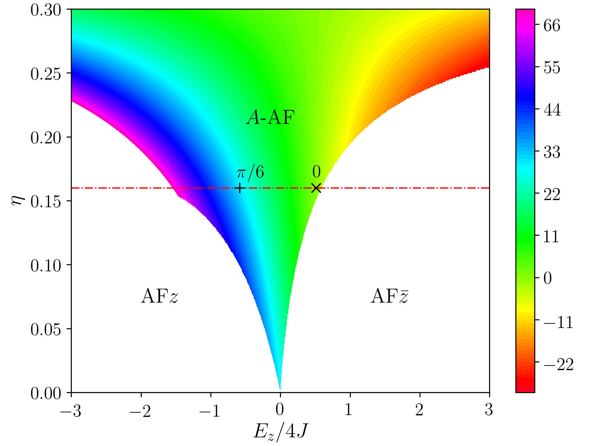
Figure 1: The mean-field phase diagram of the 3D Kugel-Khomskii model. We focus on the $A$-AF/$C$-AO spin-orbital order for which we determine the spectral function (10) occurs between two AF phases with FO order (white areas), AF$z$ (left) and AF${\bar{z}}$ (right). The color scale indicates the detuning angle $\phi$ in degrees. The values of $\phi=0$ and $\phi=\pi/6$, found at $\eta=0.16$ (red dashed line), used to investigate the spectral functions in the present study, are indicated by $\times$ and +, respectively. Note that a more complete mean-field phase diagram including possible phases described by variational wave functions with short-range order was presented before in Ref. Brzezicki et al. (2013).

In this way we generate analytical EOMs that easily allow for exact implementation of the local constraints (i.e., charge and bosons are forbidden from being at the same site simply by removing from the variational space the configurations which violate this constraint). Once generated, the EOMs form an inhomogeneous system of linearly coupled equations, which is solved numerically to yield all the Green’s functions, and in particular $G(\bm{{k}},\omega)$ from which we determine the spectral function,

$$A(\bm{{k}},\omega)=-\frac{1}{\pi}\Im G(\bm{{k}},\omega).$$ (10)

This quantity is directly measured through angle resolved photoemission spectroscopy for LaMnO₃, or inverse photoemission for KCuF₃.

We shall be interested in the spectral function obtained for the $A$-AF/$C$-AO spin-orbital order phase where both magnon and orbiton excitations may couple to the moving charge. The mean field analysis of this phase includes the energy minimization to select the optimal value of the detuning angle $\phi$, as described in Appendix A. We investigate two ground states with $\phi=0$ and $\phi={\pi}/{6}$ found at $\eta=0.16$, shown by the respective symbols in Fig. 1, and take $t\equiv 1.0$ as the energy unit.

Our method, while highly accurate and versatile, does not come without its limitations. The most important stems from the very basis of the expansion, namely the cut-off criterion being implemented in real space. As a consequence, only local processes can be treated exactly, while other interactions have to be approximated in a way compatible with this methodology. As such, this method is especially well-suited to polaronic problems, where a charge couples to bosonic excitations either on-site or on the nearest-neighboring site, such as in this paper. The most common obstacle here is the treatment of quantum fluctuations, which are not tied to the itinerant charge and are therefore completely non-local. These are generally treated by being included only in the immediate neighborhood of the electron, the logic behind this being that only then will they affect the properties of the arising QP. This works as long as the classical ground state is not too different from the true quantum ground state, i.e., the classical state is a good starting point for the expansion. This would make our method tricky to use in 1D, but any higher dimensional problem is easily treatable. Another limitation comes from the use of real space Green’s functions, which are hard to calculate already for a single electron. Treatment of multi-electron problems is an ongoing, highly challenging effort, although this is certainly true of all semi-analytical Green’s function methods. Here we only focus on single-electron spectral functions, which are relevant for photoemission spectroscopies.

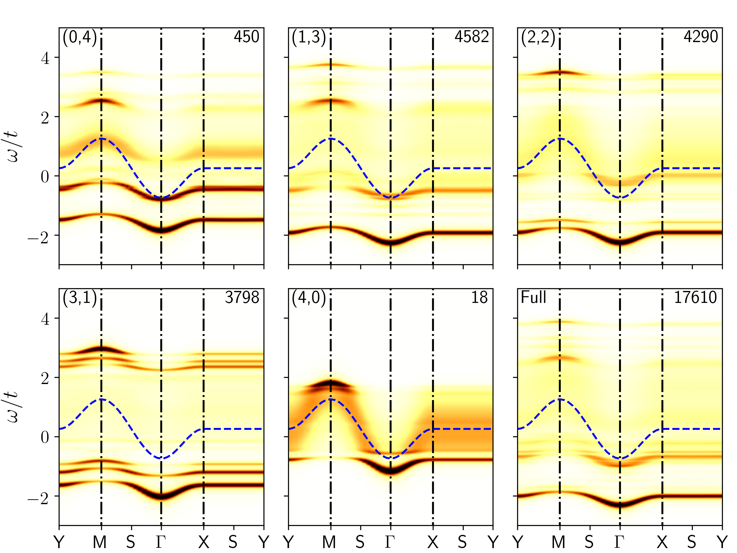
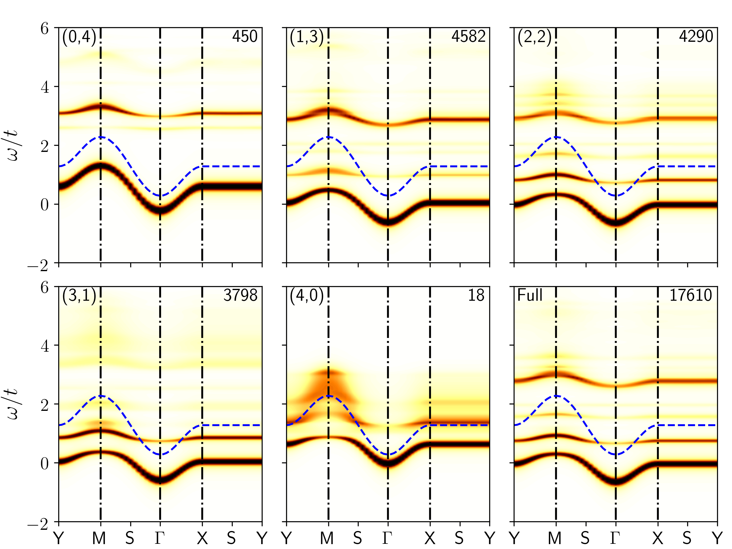
Figure 2: The spectral functions $A(\bm{{k}},\omega)$ (shown by intensity of brown/yellow color) in partial and full variational space for $\phi=0$ and $J=0.1$ (left) and $J=0.5$ (right). The dashed blue line indicates the free charge dispersion, $\epsilon_{\bm{{k}}\phi}$. The numbers in the upper-left corner indicate the maximal number of magnons and orbitons, respectively. The number in the upper-right corner gives the size of the variational space. The high-symmetry points are: $\Gamma=(0,0)$, $X=(\pi,0)$, $Y=(0,\pi)$, $S=(\pi/2,\pi/2)$, and $M=(\pi,\pi)$. Parameter: $\eta=0.16$.

IV Results and discussion

We carry out the MA calculation in the variational space defined by configurations with up to 4 bosons present. Because the calculation is done for a 3D system with full treatment of the charge coupling to bosonic degrees of freedom, the branching factor for the EOMs is far too great to allow us to include more configurations. Nevertheless, based on our previous research within similar models Bieniasz et al. (2016, 2017), we expect this choice to be sufficient for the ground state convergence to be satisfactory.

In order to distinguish the physical effects arising due to the coupling to magnons and orbitons, we have performed the calculation not only in the variational space with up to four bosons of any kind, but also in subspaces where we further restrict the number of individual bosonic flavors (e.g., up to three orbitons and up to one magnon). This allows us, to some extent, to trace the evolution of the spectral function depending on the bosonic content of the QP’s cloud in its ground state. By comparing these subspace projections to the full calculation, we can infer which bosons dominate the QP dynamics.

The spectral functions (10) were obtained for two representative mixing angles $\phi$ with coexisting $A$-AF/$C$-AO spin-orbital order, $\phi=0$ and $\phi=\pi/6$. They occur at finite Hund’s exchange $\eta>0$ near the orbital degeneracy, $E_{z}\approx 0$. We have selected $\eta=0.16$ which is representative for the AO order in KCuF₃ considered here and close to what is reported in earlier studies Oleś et al. (2005); Brzezicki et al. (2013); Liechtenstein et al. (1995); Kataoka (2004); Pavarini et al. (2008); Leonov et al. (2010). This value ensures that both the $\phi=0$ and $\phi=\pi/6$ $A$-AF/$C$-AO phases appear as the actual ground states within the range of variation of the crystal field Brzezicki et al. (2013).

The first $A$-AF/$C$-AO spin-orbital phase is obtained for $E_{z}>0$ close to the boundary between $A$-AF and AF$\bar{z}$ phases, see Fig. 1. It is characterised by symmetric and antisymmetric linear combinations of the basis orbitals, $\{|\bar{z}\rangle,|z\rangle\}$; a finite value of $E_{z}>0$ is needed because of the spin order which is AF in the $(a,b)$ planes and FM along the $c$ axis. The second spin-orbital phase discussed below has the orbital angle $\phi={\pi}/{6}$ (A), which is obtained for $E_{z}<0$, see Fig. 1. It corresponds to the other extreme characterized by the external orbital field favoring the Kugel-Khomskii orbitals.

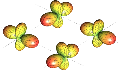
Figure 3: The in-plane orbital arrangement of the $\phi=0$ phase.

We start by analyzing the spectral functions for the $\phi=0$ phase in the Ising limit, see Fig. 2. The occupied $|\pm\rangle$ orbitals (7) form an AO state shown in Fig. 3.The Ising limit used here is defined by neglecting both spin and orbital fluctuations, i.e., discarding all terms containing operators other than $S^{z}$ or $T^{z}$. Note that the spectral function density maps are presented in a nonlinear $\propto\tanh$ scale which allows us to highlight the low amplitude states that would otherwise not be visible. The results are shown for two values of the superexchange constant, $J=0.1$ (canonical value, note that the definition of $J\equiv t^{2}/U$ does not include here the factor of 4, conventionally present in the standard $t$-$J$ model) and $J=0.5$ (weak interaction regime, this is not a physically relevant limit but it is useful for exploring the interdependence between orbitons and magnons in the system, and its effect on the polaronic physics).

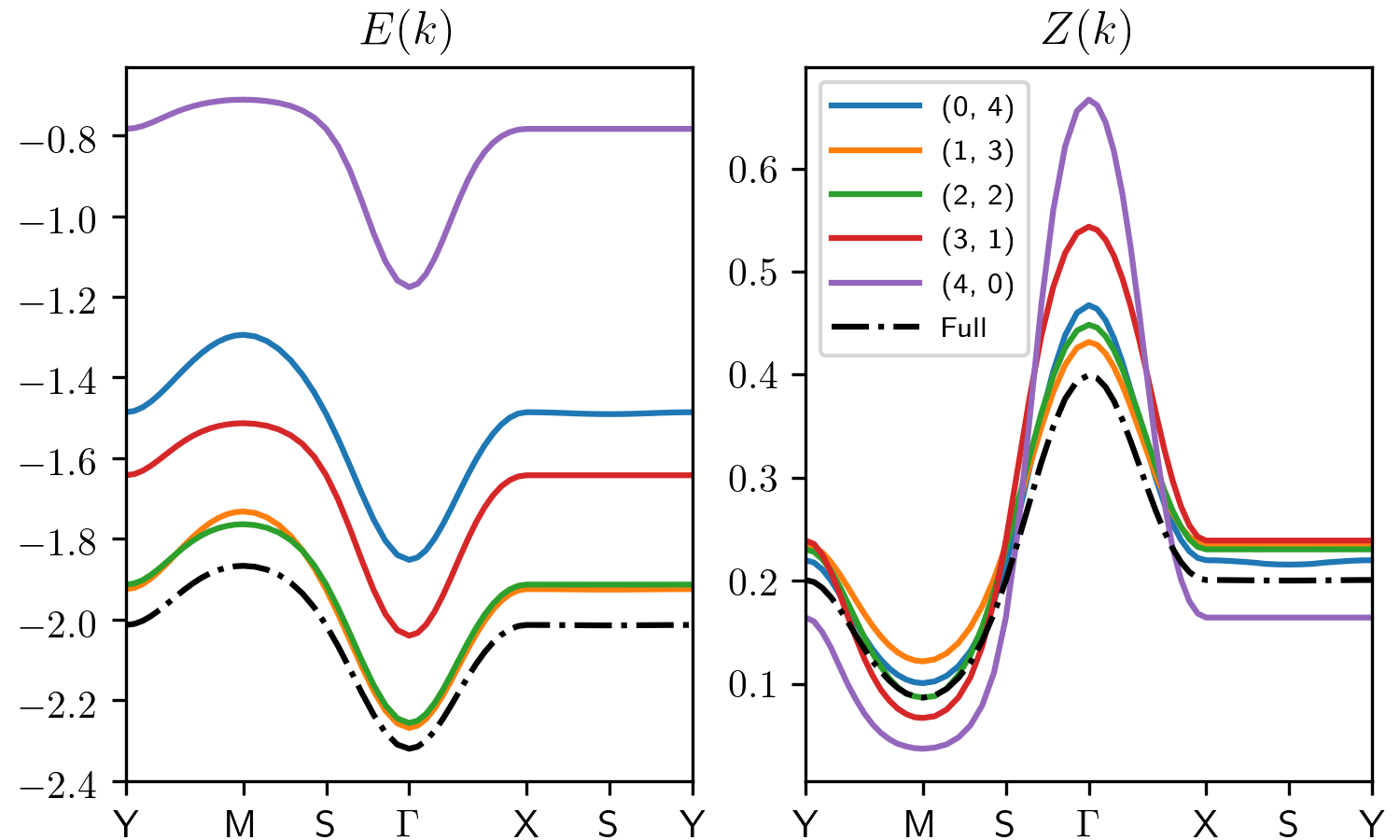
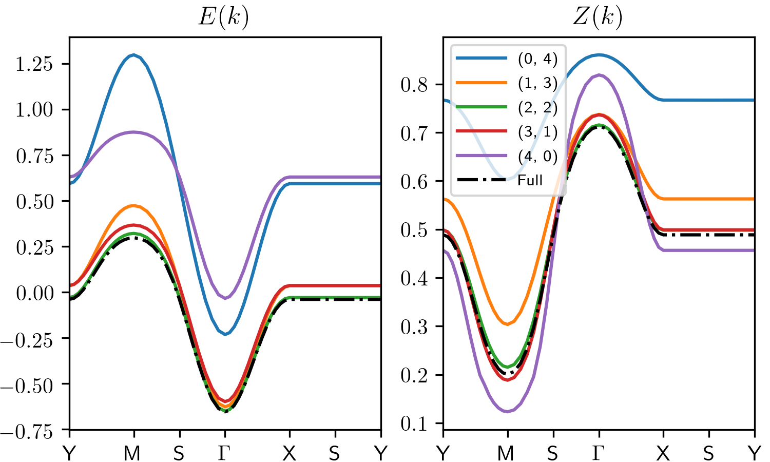
Figure 4: The extracted QP ground state energies $E(\bm{{k}})$ (left) and spectral weights $Z(\bm{{k}})$ for the full fourth order expansion (right), and the respective subspace expansions for the exchange constants $J=0.1$ (upper panels) and $J=0.5$ (lower panels). Parameter: $\eta=0.16$. Labeling conventions are the same as in Fig. 2.

Each panel in Fig. 2 is marked in the upper-left corner with the maximal number of magnons and orbitons, respectively, allowed in a given subspace, and in the upper-right corner with the size of the variational Hilbert space. The lower-right panel marked with the word “Full” presents the full expansion for up to 4 bosons (without further specifying individual bosonic flavors). The dashed blue line indicates the free charge dispersion $\epsilon_{\bm{{k}}\phi}$, and serves as a reference energy for the QP state. As expected, the dressing with bosons creates a QP which is energetically more stable than the free particle, however this comes at the cost of an increased effective mass and decreased mobility. Note that this is all consistent with standard polaronic physics. The renormalization is much smaller for the large $J$ limit. This can be easily understood because the cost of creating any boson is proportional to $J$, so the bigger $J$ is, the more expensive it is to create a big bosonic cloud. Thus, for large $J$ there will be fewer bosons in the cloud, resulting in smaller renormalization of physical properties.

Remarkably, by comparing the full results against the partial results, we can see that in the strong interaction case ($J=0.1$) the QP behaves predominantly like in the orbiton rich cases (1,3) and (2,2). To highlight this effect we extract the ground state energy and spectral weight for all these solutions and plot them against each other, see Fig. 4. As is evident, the full solution tends to include more orbitons and fewer magnons. Having said that though, a cloud consisting of only orbitons would not be sufficient to achieve the optimal QP energy, either. Thus, we can already see that this is an intrinsically spin-orbital system, where the interaction of all degrees of freedom (charge, spin, and orbital) is crucial to achieve the complete understanding of underlying physics.

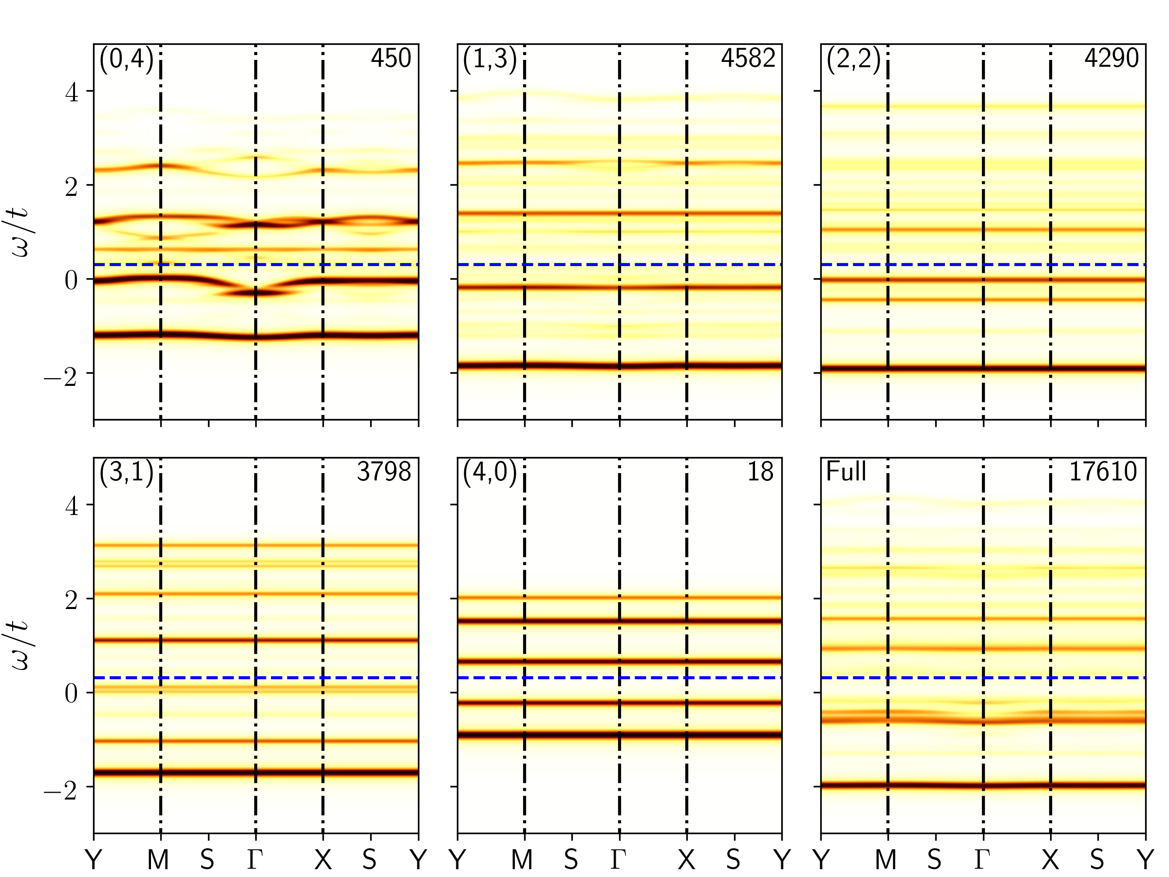
Figure 5: The full and partial spectral functions $A(\bm{{k}},\omega)$ for the $\phi=\pi/6$ phase. Parameters: $J=0.1$ and $\eta=0.16$. Notation and conventions are the same as in Fig. 2.

Even more interestingly, if we now make the same comparison for the weak interaction limit ($J=0.5$), we see that this time the QP band behaves most like the magnon-rich solutions (3,1) and (2,2). This suggests a crossover, controlled by the exchange parameter $J$, between orbiton-rich and magnon-rich QP clouds. This happens because magnons have lower energy and are cheaper to create than orbitons. In the large $J$ limit, only very few bosons are created and they are more likely to be magnons, which therefore dominate the dynamics of the resulting QP. In contrast, for small $J$ all bosons are cheap(er) and orbitons dominate by means of geometric effects, i.e., the fact that the charge can couple to them by moving in any of the three principal cubic directions, in contrast to magnons which couple only when the particle moves along the single AF $c$ direction Bieniasz et al. (2017).

Figure 5 shows the spectral functions for $\phi=\pi/6$ with $J=0.1$. The orbital order itself is depicted in Fig. 6.The first striking observation is that the bands show hardly any dispersion at all, except for the purely orbitonic solution (0,4). This is easily understood if we look at the free charge dispersion $\epsilon_{\bm{{k}}\phi}$, which vanishes for $\phi=\pi/6$, as illustrated by the flat dashed blue reference line in Fig. 5. In other words,the unrenormalized particle is completely localized, and the coupling to bosons does not change that in any substantial way. The tiny dispersion observed in the orbitonic solution is due to Trugman loops Trugman (1988), which require a 2D AO order, just like we have in this system, and the existence of at least three-boson clouds, hence its appearance in the purely orbitonic solution. In fact, a very tiny dispersion can also be seen in the (1,3) panel, however there the interference between orbitons and magnons clearly suppresses the Trugman processes Trugman (1988), again underlining the crucial role of orbiton-magnon interplay in the physics of these systems.

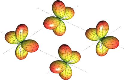
Figure 6: The in-plane orbital arrangement of the $\phi=\pi/6$ Kugel-Khomskii phase.

The lack of dispersion in this orbital phase is a straightforward consequence of a special symmetry of the orbital order in the Kugel-Khomskii state. Namely, as evident from Fig. 6, the $\phi=\pi/6$ detuning corresponds to the occupation of AO $y^{2}-z^{2}/z^{2}-x^{2}$, so the hopping process would require the charge to move from a lobe of one such orbital to the nodal point of the neighboring orbital, which is forbidden by symmetry of the wave function.

The results presented thus far point to an interesting experimental possibility. Namely, the orbital order should be discernible from a spectral experiment: the flatter the QP band, the closer the occupied orbitals should be to the $\phi=\pi/6$ phase. Naturally, determining the exact phase might not be simple, however, verifying the validity of the $\phi=\pi/6$ case to which most local density approximation (LDA) studies seem to point Kataoka (2004); Pavarini et al. (2008); Leonov et al. (2010); Binggeli and Altarelli (2004); Pavarini and Koch (2010) should be possible owing to the dispersionless character of this phase. Having said that, the issue of an insulating sample and thus strong charging during an angle resolved photoemission spectroscopy (ARPES) experiment might pose a barrier even to this verification.

There is another possibility, however, owing to the QP mass renormalization. Going back to Fig. 2 and comparing the QP vs. the free charge dispersion, we see that not only is there a difference in bandwidth between the two cases, but also the symmetry between the $\Gamma$ and $M$ points is significantly suppressed, with the QP band at the $M$ point being much flatter and having a greatly reduced spectral weight. If we would now integrate the spectrum to produce the density of states (DOS) for this system, we would see that the QP DOS for a dispersive phase should be highly asymmetric, whereas the dispersionless phase should be characterized by a sharp and completely symmetric QP DOS, as verified in Fig. 7. Thus, the orbital phase could be inferred, even if only approximately, from the shape and asymmetry of the QP DOS. In turn, the DOS can be obtained from a scanning tunneling microscope experiment for which sample charging might be less problematic.

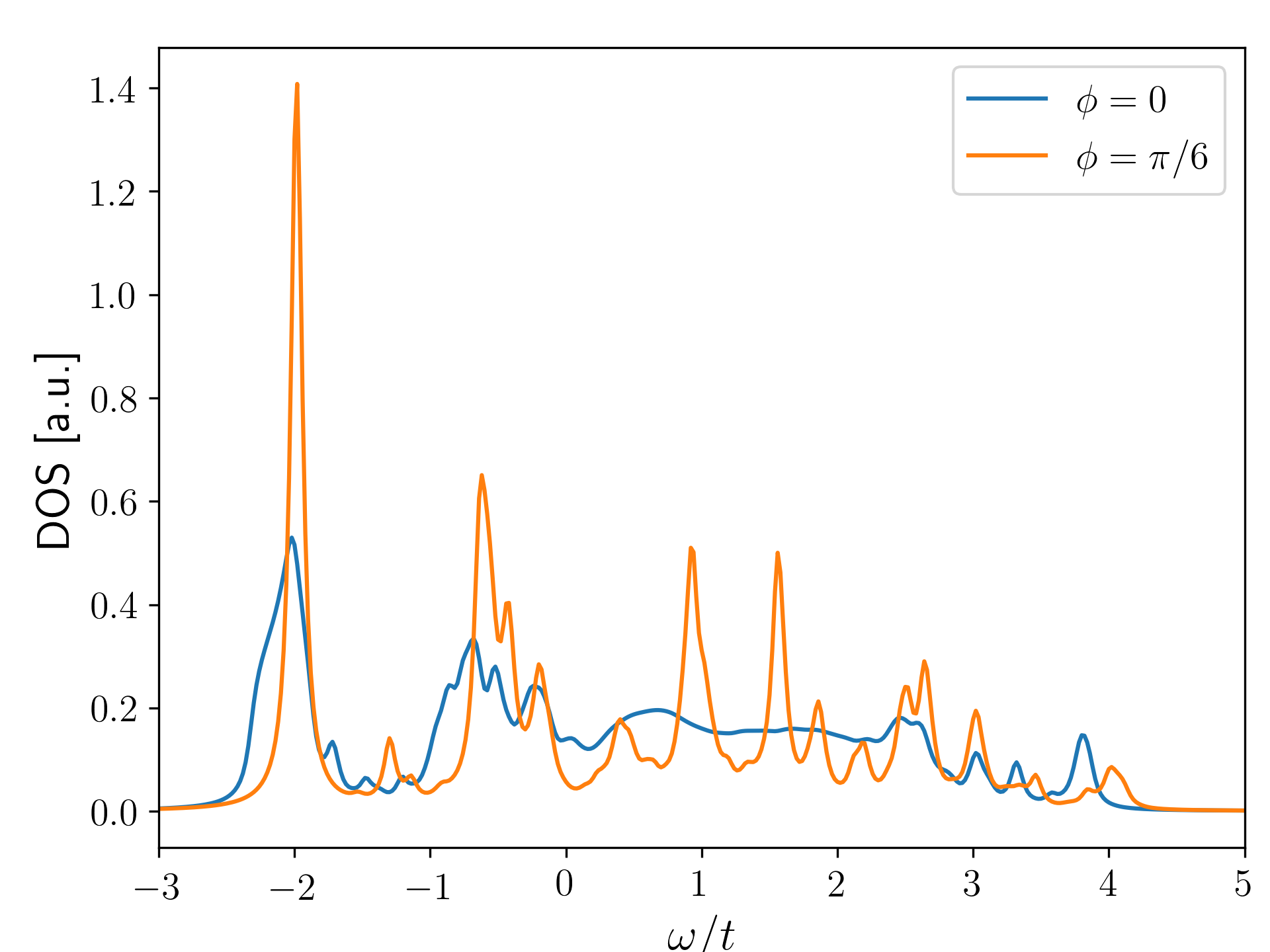
Figure 7: Comparison of the density of states for the two major orbital phases discussed in this paper, $\phi=0$ and $\phi=\pi/6$; Parameters: $J=0.1$ and $\eta=0.16$.

In all of the above we have assumed an Ising interaction, or to put it differently, that the effect of quantum fluctuations is negligible. This is a reasonable assumption because fluctuations generally are less important in higher dimensions and here we are dealing with an ostensibly 3D system. Having said that, however, the AO order can at the same time be thought as 2D and the AF order as 1D. While it has been established that the role of fluctuations for $e_{g}$ orbital pseudospin in a 2D planar subsystem is indeed negligible Bieniasz et al. (2016), the same assumption seems less justified for magnetic excitations. Apart from the dimensionality of the corresponding order, another argument is that the relative lack of importance of orbitonic fluctuations comes from the fact that the orbiton spectrum is gapped, which is not the case for magnons. This is why it is reasonable to neglect the orbital fluctuations while including magnetic fluctuations, in order to explicitly establish whether they are relevant or not.

Fortunately, magnetic fluctuations may be fairly easily included within MA by allowing arbitrary fluctuations but only in the vicinity of the propagating charge (the variational space cutoff is controlled with exactly the same cloud spatial criteria as before), since these are the only ones which will affect the QP dynamics. Fluctuations occurring far from the charge will instead only affect the nature of undoped regions far from the particle, affecting the overall energy. However, as long as the classical ground state is close enough to the true quantum state realized for a given set of parameters, this would only be reflected by a constant shift of the entire spectrum, which is not a physically significant effect.

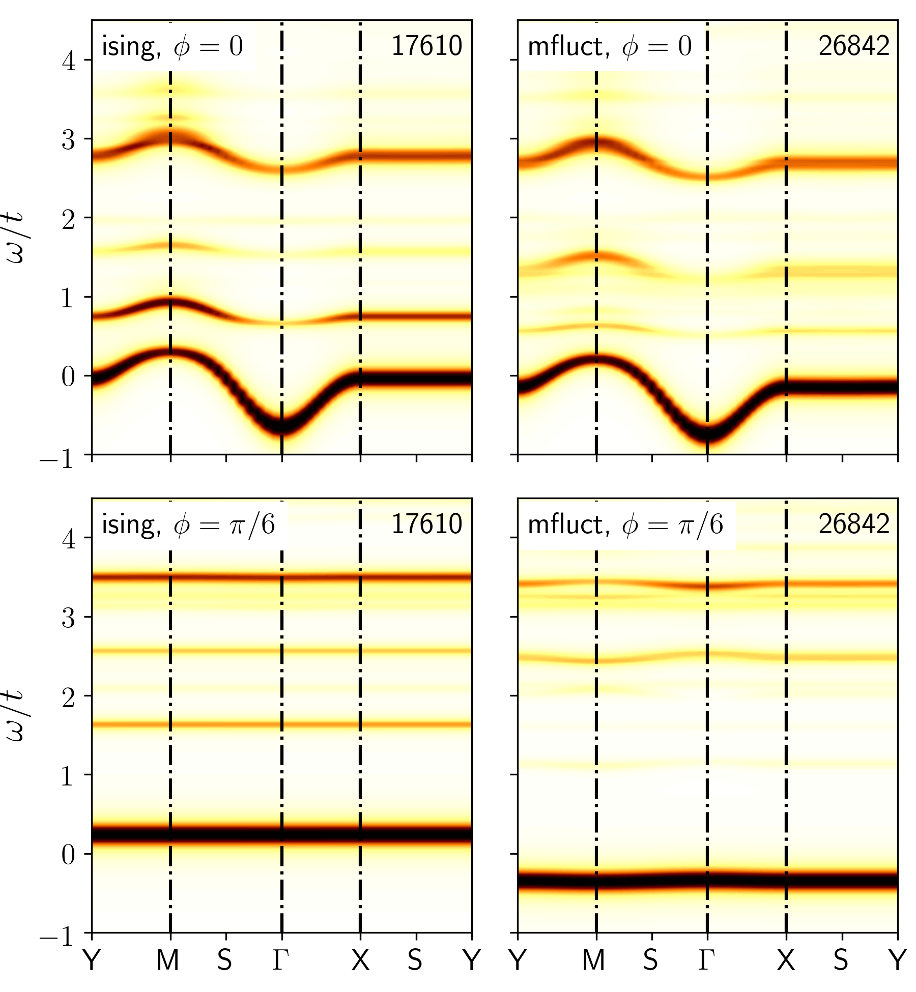
Figure 8: Comparison of the spectral functions in the Ising approximation (ising) and the one including full magnetic fluctuations (mfluct), and for the two orbital phases, $\phi=0$ and $\phi=\pi/6$. To highlight the effect we take the weak interaction regime $J=0.5$. Notation and conventions are the same as in Fig. 2. Parameter: $\eta=0.16$.

To illustrate the role of fluctuations, we present a comparison between the Ising solution and the one including local fluctuations for both angles, $\phi=0$ and $\phi=\pi/6$, see Fig. 8. As their effect proves to be rather elusive, we focus on the weak interaction limit $J=0.5$, where the changes can be more readily observed. One immediately sees the huge difference in the size of the variational spaces, even though only magnetic fluctuations (albeit in all three cubic directions) are considered here. This, however, has surprisingly little overall effect on the QP dispersion. While their effect seems more considerable for the excited states, these are likely not fully converged anyway, so that part of the spectra is not sufficiently reliable for comparison. A tiny dispersive effect can also be observed, most readily visible in the $\phi=\pi/6$ phase, however it is much too small to be of any practical importance.

There is however one interesting feature, namely the pure gain in energy experienced by the QP ground state, indicative of a stronger binding of the QP, which however does not affect its dynamical properties. In particular, while the gain for the $\phi=0$ phase is relatively small, the one observed for $\phi=\pi/6$ is considerable. This difference could be indicative of a subtle quantum effect arising from the spin-orbital coupling in the system. Clearly, the importance of the magnetic fluctuations strongly depends on the orbital phase in the system, and in particular, the fluctuations in the $\phi=\pi/6$ phase grow particularly strong. This indicates that the magnetic order becomes less classical in character, which is likely caused by the system decoupling into 1D AF chains. There is ample evidence of the actual KCuF₃ exhibiting a 1D quantum AF character Lake et al. (2005a), so this would seem to point to the actual orbital phase in that system being close to $\phi=\pi/6$, something that was long proposed based on electronic structure calculations using LDA. Here we were able to arrive at similar conclusions through indirect means and by a completely different methodology.

V Summary and Conclusions

We have developed an effective spin-orbital superexchange model for an $e_{g}^{3}$ system, and computed the single-polaron spectrum resulting when a single charge is doped in the system by using the semi-analytical, variational momentum average method for calculating Green’s functions. This allowed us not only to obtain the relevant spectral functions, but also to gain insight into the nature of the magnetic and orbital order in the system. Thus we were able to demonstrate a number of subtle quantum effects arising from the interaction between the charge, orbital, and magnetic degrees of freedom.

One such effects is the change of the character of the polaronic quasiparticle cloud from being dominated by orbitons to being dominated by magnons; this is controlled by the strength of the superexchange interaction $J$. This behavior, although only a theoretical prediction due to the impossibility of experimentally tuning the parameter $J$ in such a wide range of values, nonetheless points towards a strong interplay between orbital and magnetic degrees of freedom in this model. It should come as no surprise, then, that their intermingling should also crop up in other properties of the system, some of which might be more readily accessible to experiment.

One possible experimental consequence lies in the quasiparticle dispersion being strongly dependent on the orbital order in the system which, coupled with the polaronic suppression of the symmetry between the $\Gamma$ and $M$ points of the Brillouin zone, suggests that the quasiparticle density of states should be particularly sensitive to the orbital order in these systems. In turn, this would point towards Scanning Tunneling Microscopy as a promising tool for an experimental probe of the orbital order type. We thus propose that the orbital order could be inferred by investigating the amplitude to width ratio and the asymmetry of the density of states peaks.

Finally, we point out that the orbital order around the detuning angle $\phi=\pi/6$ seems to drive the magnetic system closer towards the 1D AF chain. Indeed, the already available results of neutron scattering experiments Lake et al. (2005a) demonstrate a nearly ideal 1D spin liquid behavior. We suggest that this is a strong indication that the orbital order in KCuF₃ is likely to be close to $\phi=\pi/6$.

Appendix A The mean field ground state

In this Section we provide the more technical details concerning the derivation of the effective polaronic spin-orbital model that is the basis of our calculation. In order to find the classical orbital ground state, we parametrize the orbital basis in terms of a standard rotation of the $\{\bar{z},z\}$ basis. However, since the reference, field-free order is composed of alternating $\lvert\pm\rangle$ states (7), the rotation is most conveniently parametrized with an angle $\pm(\pi/2+\phi)$, where the sign depends on the orbital sublattice,

$$\lvert\phi_{A}\rangle = \cos\left(\frac{\pi}{4}+\frac{\phi}{2}\right)\lvert\bar{z}\rangle+\sin\left(\frac{\pi}{4}+\frac{\phi}{2}\right)\lvert z\rangle,$$

$$\lvert\phi_{B}\rangle = \cos\left(\frac{\pi}{4}+\frac{\phi}{2}\right)\lvert\bar{z}\rangle-\sin\left(\frac{\pi}{4}+\frac{\phi}{2}\right)\lvert z\rangle.$$ (11)

This choice also serves to transform the underlying AO order to an FO order, effectively eliminating the bipartite division of the lattice in the reference state. It should be stressed that this operation does not affect the actual ground state, it merely changes its representation to one that is more convenient—it spares us the trouble of distinguishing between bosons on different sublattices (cf. Ref. Martínez and Horsch, 1991).Now $\phi$ will indicate a detuning from the field-free orbital order, and the angle between the occupied orbitals on the two sublattices will be $2\phi$ (i.e., in general, the bases on different sublattices will not be mutually orthogonal).

To find the relation between the orbital field $E_{z}$ and the detuning angle $\phi$ in Eqs. (A), we start by writing out the superexchange Hamiltonian in the new basis:

$$\mathcal{H}_{\mathrm{I}}^{\perp} =J\sum_{\langle ij\rangle\perp c}\left(A_{\eta}\bm{{S}}_{i}\cdot\bm{{S}}_{j}+\tfrac{1}{4}B_{\eta}\right)\left\{\tfrac{2C_{\eta}}{A_{\eta}}-1-(2\cos 2\phi+1)\,T_{i}^{z}T_{j}^{z}-(2\cos 2\phi-1)\,T_{i}^{x}T_{j}^{x}\right.$$

$$\qquad\left.+2e^{i\bm{{Q}}\bm{{R}}_{i}}\sin 2\phi\,(T_{i}^{z}T_{j}^{x}-T_{i}^{x}T_{j}^{z})\mp\sqrt{3}\,(T_{i}^{x}T_{j}^{z}+T_{i}^{z}T_{j}^{x})\right\},$$ (12a)

$$\mathcal{H}_{\mathrm{I}}^{\parallel} =2J\sum_{\langle ij\rangle\parallel c}\left(A_{\eta}\bm{{S}}_{i}\cdot\bm{{S}}_{j}+\tfrac{1}{4}B_{\eta}\right)\left\{\tfrac{C_{\eta}}{A_{\eta}}-\tfrac{1}{2}+2\sin^{2}\phi\,T_{i}^{z}T_{j}^{z}+2\cos^{2}\phi\,T_{i}^{x}T_{j}^{x}-e^{i\bm{{Q}}\bm{{R}}_{i}}\sin 2\phi\,(T_{i}^{x}T_{j}^{z}+T_{i}^{z}T_{j}^{x})\right\},$$ (12b)

$$\mathcal{H}_{\mathrm{II}}^{\perp} =-JC_{\eta}\sum_{\langle ij\rangle\perp c}\left(\bm{{S}}_{i}\cdot\bm{{S}}_{j}-\tfrac{1}{4}\right)\left\{\left[\sin\phi\,(T_{i}^{z}+T_{j}^{z})\mp\sqrt{3}e^{i\bm{{Q}}\bm{{R}}_{i}}\cos\phi\right](T_{i}^{z}-T_{j}^{z})\right.$$

$$\qquad\left.-e^{i\bm{{Q}}\bm{{R}}_{i}}\cos\phi\,(T_{i}^{x}-T_{j}^{x})\mp\sqrt{3}\sin\phi\,(T_{i}^{x}+T_{j}^{x})\right\},$$ (12c)

$$\mathcal{H}_{\mathrm{II}}^{\parallel} =2JC_{\eta}\sum_{\langle ij\rangle\parallel c}\left(\bm{{S}}_{i}\cdot\bm{{S}}_{j}-\tfrac{1}{4}+\tfrac{E_{z}}{4JC_{\eta}}\right)\left[\sin\phi\,(T_{i}^{z}+T_{j}^{z})-e^{i\bm{{Q}}\bm{{R}}_{i}}\cos\phi\,(T_{i}^{x}+T_{j}^{x})\right],$$ (12d)

where the last term incorporates the orbital field $\mathcal{H}_{z}$. Here, $\bm{{Q}}=(\pi,\pi,0)$ is the ordering vector for the $C$-AO state, and the resulting phase factor encodes the alternating nature of the orbital order. The symbol $\perp/\parallel$ refers to the cubic directions with respect to the $c$-axis. Note that the various superexchange terms of Eq. (2) have been split into terms quadratic in $\{T_{i}^{z}\}$ operators ($\mathcal{H}_{\mathrm{I}}$) and linear in $\{T_{i}^{z}\}$ operators ($\mathcal{H}_{\mathrm{II}}$). The Hund’s exchange (4) is now encoded in the three prefactors (if $\eta=0$, one finds $A_{0}=B_{0}=C_{0}=1$):

$$A_{\eta}=\frac{1-\eta}{(1+\eta)(1-3\eta)},$$ (13a)

$$B_{\eta}=\frac{1+3\eta}{(1+\eta)(1-3\eta)},$$ (13b)

$$C_{\eta}=\frac{1}{1-\eta^{2}},$$ (13c)

which themselves result from various combinations of the $r_{i}$ multiplet parameters listed above. Note that the exchange Hamiltonian has also been shifted in energy so that the Ising energy for the ground state of the system is set to zero. This is done merely for reasons of convenience, so that the excitation energies are easier to track once we start considering excitations in the system.

Next we evaluate the mean field energy assuming the classical ground state to be A-AF/C-AO, as is known to be the case in KCuF₃. We find:

$$E_{\mathrm{MF}}=\frac{1}{4}J(B_{\eta}-A_{\eta})\sin^{2}\phi-\frac{1}{8}J(A_{\eta}+B_{\eta})(2\cos 2\phi+1)\\ -J\left(C_{\eta}-\frac{E_{z}}{2J}\right)\sin\phi.$$ (14)

This expression is then minimized with respect to the detuning angle $\phi$, yielding the relation

$$E_{z}=J\left[2C_{\eta}-\left(A_{\eta}+3B_{\eta}\right)\sin\phi\right].$$ (15)

This identity can now be used to eliminate $E_{z}$ from the Hamiltonian by replacing it with the detuning angle $\phi$. Note that if we now set $\phi=0$, we will, seemingly paradoxically, get $E_{z}=2JC_{\eta}$, i.e., a finite orbital field corresponding to the field-free case. This is due to the fact that the superexchange Hamiltonian already includes terms linear in pseudospin operators which behave like an orbital field, and the external field works to compensate these terms. In other words, the exchange Hamiltonian breaks cubic symmetry by itself, and the above estimate is the orbital field needed to restore it. On the other hand, the case $E_{z}=0$ corresponds to $\phi=\pi/6$ in the 2D orbital model Czarnik et al. (2017), which is the Kugel-Khomskii state composed of alternating $y^{2}-z^{2}/z^{2}-x^{2}$ states. These two limits are commonly cited as the extreme possibilities for the orbital order in this system. The actual orbital order realized in the system will be bounded by these two extremes, and in fact could be, to some extent, tuned by means of an axial pressure $\propto E_{z}$ applied along the $c$ axis.

Appendix B Fermion-boson polaronic model

To go beyond the mean field ground state, we derive the effective Hamiltonian transforming the physics of a single charge doped into a spin-orbital model to a fermion-boson many-body problem. To that end, we transform the kinetic Hamiltonian to the same basis as the one considered in the last Section, so that the entire model is expressed in compatible representations. This leads to

$$\mathcal{H}_{t}^{\perp} =-\frac{t}{4}\sum_{\langle ij\rangle\perp c,\sigma}\left\{\left[(1-2\sin\phi)d_{i\sigma 0}^{{\dagger}}d_{j\sigma 0}\right.\right.$$

$$\qquad-2e^{i\bm{{Q}}\bm{{R}}_{i}}\cos\phi\,(d_{i\sigma 0}^{{\dagger}}d_{j\sigma 1}-d_{i\sigma 1}^{{\dagger}}d_{j\sigma 0})$$

$$\qquad\mp\sqrt{3}\,(d_{i\sigma 0}^{{\dagger}}d_{j\sigma 1}+d_{i\sigma 1}^{{\dagger}}d_{j\sigma 0})$$

$$\qquad\left.\left.-(1+2\sin\phi)d_{i\sigma 1}^{{\dagger}}d_{j\sigma 1}\right]+\mathrm{H.c.}\right\}\,,$$ (16a)

$$\mathcal{H}_{t}^{\parallel} =-\frac{t}{2}\sum_{\langle ij\rangle\parallel c,\sigma}\left\{\left[(1+\sin\phi)d_{i\sigma 0}^{{\dagger}}d_{j\bar{\sigma}0}\right.\right.$$

$$\qquad-e^{i\bm{{Q}}\bm{{R}}_{i}}\cos\phi\,(d_{i\sigma 0}^{{\dagger}}d_{j\bar{\sigma}1}+d_{i\sigma 1}^{{\dagger}}d_{j\bar{\sigma}0})$$

$$\qquad\left.\left.-(1-\sin\phi)\,d_{i\sigma 1}^{{\dagger}}d_{j\bar{\sigma}1}\right]+\mathrm{H.c.}\right\}\,,$$ (16b)

where the 0 (1) indices denote the ground (excited) orbital states, respectively.

Finally, following Martínez and Horsch Martínez and Horsch (1991), we represent the spin and orbital degrees of freedom using a slave boson representation. This is achieved by expanding the (pseudo)spin operators around the assumed mean field ground state by means of a Holstein-Primakoff transformation,

$$\begin{aligned} d_{i\uparrow 0}^{{\dagger}}&=f_{i}^{{\dagger}},\\ d_{i\downarrow 0}^{{\dagger}}&=f_{i}^{{\dagger}}b_{i},\end{aligned} \begin{aligned} d_{i\uparrow 1}^{{\dagger}}&=f_{i}^{{\dagger}}a_{i},\\ d_{i\downarrow 1}^{{\dagger}}&=f_{i}^{{\dagger}}a_{i}b_{i},\end{aligned}$$ (17)

where $b_{i}^{{\dagger}}$ creates a spin excitation at site $i$, $a_{i}^{{\dagger}}$ creates an orbital excitation, and $f_{i}^{{\dagger}}$ creates a spinless fermion which represents the charge degree of freedom, where $0$ indicates the site $i$ in the ground state, while $1$ means that the respective site hosts an excited state. Thus, a charge can be added to the system only if it is locally in its (classical) ground state, otherwise if a boson occupied the considered site, first it has to be removed before the charge can be added. Also note that the on-site bosonic Hilbert space is restricted to $(2S+1)$ states, and since both the spin and the pseudospin have length $\nicefrac{{1}}{{2}}$, each site can host not more than one boson of each kind. This local constraint applies to every site and is fully taken into account in our calculations through the variational technique employed.

The exchange Hamiltonian also has to be transformed into its bosonic representation, which is done by means of the Holstein-Primakoff transformation of the spin operators,

$$S_{i}^{z}=\frac{1}{2}-b_{i}^{{\dagger}}b_{i},\!\quad S_{i}^{+}=\sqrt{1-b_{i}^{{\dagger}}b_{i}}\,b_{i},\!\quad S_{i}^{-}=b_{i}^{{\dagger}}\sqrt{1-b_{i}^{{\dagger}}b_{i}},$$ (18)

and similarly for the pseudospin operators, but in terms of orbiton operators $\left\{a_{i},a_{i}^{{\dagger}}\right\}$. There are two issues that are still worth pointing out concerning this transformation. Firstly, the $S_{i}^{z}$ operators are the ones that most readily introduce higher order terms into the Hamiltonian, and thus are principally responsible for inter-bosonic interactions, which can have profound effects for low-dimensional physics Bieniasz et al. (2018) but which nonetheless are all too often neglected in techniques reetalying on the LSW approximation. It is therefore worth mentioning that in our variational method this part of the transformation is not strictly necessary, as the $S_{i}^{z}$ operators merely “count” the Ising energy of the bosons and thus their effect can be discerned directly from the configuration of the system. Or, to put it differently, in our method it would actually be more cumbersome (although possible) to calculate the energy in the LSW approximation than it is to do it exactly.

Secondly, the square root factors in the fluctuation operators $S_{i}^{\pm}$ are conventionally treated by Taylor expansion and truncation at second order, to be consistent with the LSW approximation. However, here again, one should realize that these factors merely serve to impose the restriction of a single boson per site, and thus this constraint can be taken into account by excluding from the variational space the configurations which violate it. Therefore, with our variational technique we can bosonize the exchange interactions without the need to abandon any of the inter-bosonic interactions or constraints.

Applying these transformations decouples the original fermions into their constituent charge, spin, and orbital degrees of freedom. The free charge propagation $\mathcal{H}_{t}$, as well as its coupling to the bosonic degrees of freedom, will now be described by the kinetic Hamiltonian, which after the above transformations reads,

$$\mathcal{H}_{t}=\mathcal{T}+\mathcal{V}^{\perp}_{t}+\mathcal{V}^{\parallel}_{t}\,,$$ (19)

where:

$$\mathcal{T} =-\frac{t}{4}\sum_{\langle ij\rangle\perp c}\left(1-2\sin\phi\right)\left(f_{i}^{{\dagger}}f_{j}+\mathrm{H.c.}\right)=\sum_{\bm{{k}}}\epsilon_{\bm{{k}}\phi}f_{\bm{{k}}}^{{\dagger}}f_{\bm{{k}}},$$ (20a)

$$\mathcal{V}^{\perp}_{t} =\frac{t}{4}\sum_{\langle ij\rangle\perp c}\left\{\left[2e^{i\bm{{Q}}\bm{{R}}_{i}}\cos\phi(a_{j}^{{\dagger}}-a_{i})\pm\sqrt{3}(a_{j}^{{\dagger}}+a_{i})+(1+2\sin\phi)a_{j}^{{\dagger}}a_{i}\right](1+b_{i}b_{j}^{{\dagger}})f_{i}^{{\dagger}}f_{j}+\mathrm{H.c.}\right\}$$

$$-\frac{t}{4}\sum_{\langle ij\rangle\perp c}\left[(1-2\sin\phi)b_{i}b_{j}^{{\dagger}}f_{i}^{{\dagger}}f_{j}+\mathrm{H.c.}\right],$$ (20b)

$$\mathcal{V}^{\parallel}_{t} =-\frac{t}{2}\sum_{\langle ij\rangle\parallel c}\left\{\left[(1+\sin\phi)-e^{i\bm{{Q}}\bm{{R}}_{i}}\cos\phi(a_{i}+a_{j}^{{\dagger}})-(1-\sin\phi)a_{i}a_{j}^{{\dagger}}\right]\,(b_{i}+b_{j}^{{\dagger}})f_{i}^{{\dagger}}f_{j}+\mathrm{H.c.}\right\},$$ (20c)

and $\epsilon_{\bm{{k}}\phi}=-\frac{1}{2}t(1-2\sin\phi)(\cos k_{x}+\cos k_{y})$ is the free electron dispersion. We emphasize that it depends on the orbital order (A) through the angle $\phi$, and vanishes when $\phi=\pi/6$. The free charge hopping term $\mathcal{T}$ is restricted to the $ab$ planes because of the magnetic order alternating in the perpendicular direction $c$, which thus requires creation or annihilation of a magnon when the charge hops in that direction.

The remaining terms couple the charge to the bosonic degrees of freedom, and some of them are high-order many-body interactions, sometimes coupling the charge to multiple bosons at the same time. Treating these interactions with a technique relying on the LSW approximation would be impossible, whereas this can be done within the variational momentum average approach, as presented in Sec. IV.

References

- Chao et al. (1977) K. A. Chao, J. Spałek, and A. M. Oleś, J. Phys. C 10, L271 (1977).
- Trugman (1988) S. A. Trugman, Phys. Rev. B 37, 1597 (1988).
- Liu and Manousakis (1992) Z. Liu and E. Manousakis, Phys. Rev. B 45, 2425 (1992).
- Manousakis (2007) E. Manousakis, Phys. Rev. B 75, 035106 (2007).
- Grusdt et al. (2018) F. Grusdt, M. Kánasz-Nagy, A. Bohrdt, C. S. Chiu, G. Ji, M. Greiner, D. Greif, and E. Demler, Phys. Rev. X 8, 011046 (2018).
- Kane et al. (1989) C. L. Kane, P. A. Lee, and N. Read, Phys. Rev. B 39, 6880 (1989).
- Martínez and Horsch (1991) G. Martínez and P. Horsch, Phys. Rev. B 44, 317 (1991).
- Lee et al. (2006) P. A. Lee, N. Nagaosa, and X.-G. Wen, Rev. Mod. Phys. 78, 17 (2006).
- Kugel and Khomskii (1982) K. I. Kugel and D. I. Khomskii, Sov. Phys. Usp. 25, 231 (1982).
- Tokura and Nagaosa (2000) Y. Tokura and N. Nagaosa, Science 288, 462 (2000).
- Oleś (1983) A. M. Oleś, Phys. Rev. B 28, 327 (1983).
- Hoshino and Werner (2016) S. Hoshino and P. Werner, Phys. Rev. B 93, 155161 (2016).
- Feiner et al. (1997) L. F. Feiner, A. M. Oleś, and J. Zaanen, Phys. Rev. Lett. 78, 2799 (1997).
- Ishihara et al. (1997) S. Ishihara, J. Inoue, and S. Maekawa, Phys. Rev. B 55, 8280 (1997).
- Feiner and Oleś (1999) L. F. Feiner and A. M. Oleś, Phys. Rev. B 59, 3295 (1999).
- Snamina and Oleś (2018) M. Snamina and A. M. Oleś, Phys. Rev. B 97, 104417 (2018).
- Khaliullin and Maekawa (2000) G. Khaliullin and S. Maekawa, Phys. Rev. Lett. 85, 3950 (2000).
- Khaliullin et al. (2001) G. Khaliullin, P. Horsch, and A. M. Oleś, Phys. Rev. Lett. 86, 3879 (2001).
- Khaliullin et al. (2004) G. Khaliullin, P. Horsch, and A. M. Oleś, Phys. Rev. B 70, 195103 (2004).
- Khaliullin (2005) G. Khaliullin, Prog. Theor. Phys. Suppl. 160, 155 (2005).
- Oleś et al. (2005) A. M. Oleś, G. Khaliullin, P. Horsch, and L. F. Feiner, Phys. Rev. B 72, 214431 (2005).
- Chaloupka and Khaliullin (2008) J. Chaloupka and G. Khaliullin, Phys. Rev. Lett. 100, 016404 (2008).
- Horsch et al. (2008) P. Horsch, A. M. Oleś, L. F. Feiner, and G. Khaliullin, Phys. Rev. Lett. 100, 167205 (2008).
- Normand and Oleś (2008) B. Normand and A. M. Oleś, Phys. Rev. B 78, 094427 (2008).
- Normand (2011) B. Normand, Phys. Rev. B 83, 064413 (2011).
- Chaloupka and Oleś (2011) J. Chaloupka and A. M. Oleś, Phys. Rev. B 83, 094406 (2011).
- Sirker et al. (2008) J. Sirker, A. Herzog, A. M. Oleś, and P. Horsch, Phys. Rev. Lett. 101, 157204 (2008).
- Herzog et al. (2011) A. Herzog, P. Horsch, A. M. Oleś, and J. Sirker, Phys. Rev. B 83, 245130 (2011).
- Brzezicki et al. (2015) W. Brzezicki, A. M. Oleś, and M. Cuoco, Phys. Rev. X 5, 011037 (2015).
- Brzezicki (2019) W. Brzezicki, arXiv:1904.11772 (2019).
- van den Brink et al. (2000) J. van den Brink, P. Horsch, and A. M. Oleś, Phys. Rev. Lett. 85, 5174 (2000).
- Ishihara et al. (2005) S. Ishihara, Y. Murakami, T. Inami, K. Ishii, J. Mizuki, K. Hirota, S. Maekawa, and Y. Endoh, New J. Phys. 7, 119 (2005).
- Ishihara (2005) S. Ishihara, Phys. Rev. Lett. 94, 156408 (2005).
- Daghofer et al. (2004) M. Daghofer, A. M. Oleś, and W. von der Linden, Phys. Rev. B 70, 184430 (2004).
- Wohlfeld et al. (2009) K. Wohlfeld, A. M. Oleś, and P. Horsch, Phys. Rev. B 79, 224433 (2009).
- Berciu (2009) M. Berciu, Physics 2, 55 (2009).
- Okazaki and Suemune (1961) A. Okazaki and Y. Suemune, J. Phys. Soc. Japan 16, 176 (1961).
- Zhou and Goodenough (2006) J.-S. Zhou and J. B. Goodenough, Phys. Rev. Lett. 96, 247202 (2006).
- Kimura et al. (2003) T. Kimura, S. Ishihara, H. Shintani, T. Arima, K. T. Takahashi, K. Ishizaka, and Y. Tokura, Phys. Rev. B 68, 060403 (2003).
- Lake et al. (2005a) B. Lake, D. A. Tennant, C. D. Frost, and S. E. Nagler, Nature Mat. 4, 329 (2005a).
- Lake et al. (2005b) B. Lake, D. A. Tennant, and S. E. Nagler, Phys. Rev. B 71, 134412 (2005b).
- Jonker and Van Santen (1950) G. H. Jonker and J. H. van Santen, Physica 16, 337 (1950).
- Tokura (2006) Y. Tokura, Reports on Progress in Physics 69, 797 (2006).
- Rościszewski and Oleś (2019) K. Rościszewski and A. M. Oleś, Phys. Rev. B 99, 155108 (2019).
- Bała et al. (2001) J. Bała, G. A. Sawatzky, A. M. Oleś, and A. Macridin, Phys. Rev. Lett. 87, 067204 (2001).
- Krüger et al. (2004) R. Krüger, B. Schulz, S. Naler, R. Rauer, D. Budelmann, J. Bäckström, K. H. Kim, S.-W. Cheong, V. Perebeinos, and M. Rübhausen, Phys. Rev. Lett. 92, 097203 (2004).
- Kim et al. (2002) M. W. Kim, J. H. Jung, K. H. Kim, H. J. Lee, J. Yu, T. W. Noh, and Y. Moritomo, Phys. Rev. Lett. 89, 016403 (2002).
- Kovaleva et al. (2010) N. N. Kovaleva, A. M. Oleś, A. M. Balbashov, A. Maljuk, D. N. Argyriou, G. Khaliullin, and B. Keimer, Phys. Rev. B 81, 235130 (2010).
- Snamina and Oleś (2019) M. Snamina and A. M. Oleś, New Journal of Physics 21, 023018 (2019).
- Kuneš et al. (2010) J. Kuneš, I. Leonov, M. Kollar, K. Byczuk, V. Anisimov, and D. Vollhardt, Eur. Phys. J. Special Topics 180, 5 (2010).
- Feiner and Oleś (2005) L. F. Feiner and A. M. Oleś, Phys. Rev. B 71, 144422 (2005).
- Oleś et al. (2000) A. M. Oleś, L. F. Feiner, and J. Zaanen, Phys. Rev. B 61, 6257 (2000).
- Brzezicki et al. (2012) W. Brzezicki, J. Dziarmaga, and A. M. Oleś, Phys. Rev. Lett. 109, 237201 (2012).
- Czarnik et al. (2017) P. Czarnik, J. Dziarmaga, and A. M. Oleś, Phys. Rev. B 96, 014420 (2017).
- Bieniasz et al. (2018) K. Bieniasz, P. Wrzosek, A. M. Oleś, and K. Wohlfeld, arXiv:1809.07120 (2018).
- Berciu (2006) M. Berciu, Phys. Rev. Lett. 97, 036402 (2006).
- Marchand et al. (2010) D. J. J. Marchand, G. De Filippis, V. Cataudella, M. Berciu, N. Nagaosa, N. V. Prokof’ev, A. S. Mishchenko, and P. C. E. Stamp, Phys. Rev. Lett. 105, 266605 (2010).
- Berciu and Fehske (2011) M. Berciu and H. Fehske, Phys. Rev. B 84, 165104 (2011).
- Ebrahimnejad et al. (2016) H. Ebrahimnejad, G. A. Sawatzky, and M. Berciu, J. Phys.: Cond. Mat. 28, 105603 (2016).
- Bieniasz et al. (2016) K. Bieniasz, M. Berciu, M. Daghofer, and A. M. Oleś, Phys. Rev. B 94, 085117 (2016).
- Bieniasz et al. (2017) K. Bieniasz, M. Berciu, and A. M. Oleś, Phys. Rev. B 95, 235153 (2017).
- Brzezicki et al. (2013) W. Brzezicki, J. Dziarmaga, and A. M. Oleś, Phys. Rev. B 87, 064407 (2013).
- Liechtenstein et al. (1995) A. I. Liechtenstein, V. I. Anisimov, and J. Zaanen, Phys. Rev. B 52, R5467 (1995).
- Kataoka (2004) M. Kataoka, J. Phys. Soc. Jpn. 73, 1326 (2004).
- Pavarini et al. (2008) E. Pavarini, E. Koch, and A. I. Lichtenstein, Phys. Rev. Lett. 101, 266405 (2008).
- Leonov et al. (2010) I. Leonov, D. Korotin, N. Binggeli, V. I. Anisimov, and D. Vollhardt, Phys. Rev. B 81, 075109 (2010).
- Binggeli and Altarelli (2004) N. Binggeli and M. Altarelli, Phys. Rev. B 70, 085117 (2004).
- Pavarini and Koch (2010) E. Pavarini and E. Koch, Phys. Rev. Lett. 104, 086402 (2010).