Detection of multiple stellar populations in extragalactic massive clusters with JWST

The discovery both through spectroscopy and photometry of multiple stellar populations (multiple in the sense of non homogeneous chemical abundances, with specific patterns of variations of a few light elements) in Galactic globular clusters, and in Magellanic Clouds’ massive intermediate-age and old clusters, has led to a major change in our views about the formation of these objects. To date, none of the proposed scenarios is able to explain quantitatively all chemical patterns observed in individual clusters, and an extension of the study of multiple populations to resolved extragalactic massive clusters beyond the Magellanic Clouds would be welcome, for it would enable to investigate and characterize the presence of multiple populations in different environments and age ranges. To this purpose, the James Webb Space Telescope can potentially play a major role. On the one hand, the James Webb Space Telescope promises direct observations of proto-globular cluster candidates at high redshift; on the other hand, it can potentially push to larger distances the sample of resolved clusters with detected multiple populations. In this paper we have addressed this second goal. Using theoretical stellar spectra and stellar evolution models, we have investigated the effect of multiple population chemical patterns on synthetic magnitudes in the James Webb Space Telescope infrared NIRCam filters. We have identified the colours $(F150W-F460M)$, $(F115W-F460M)$ and pseudocolours $C_{F150W,F460M,F115W}=(F150W-F460M)-(F460M-F115W)$, $C_{F150W,F277W,F115W}=(F150W-F277W)-(F277W-F115W)$, as diagnostics able to reveal the presence of multiple populations along the red giant branches of old and intermediate age clusters. Using the available on-line simulator for the NIRCam detector, we have estimated that multiple populations can be potentially detected –depending on the exposure times, exact filter combination used, plus the extent of the abundance variations and the cluster [Fe/H]– out to a distance of $\sim$5 Mpc (approximately the distance to the M83 group).

1 Introduction

The formation of globular clusters (GCs) is still an open problem (see, e.g., Forbes et al., 2018, for a very recent review), made somewhat more complex by the discovery that GCs do not host single-age, single chemical composition populations, as widely believed until not so long ago. Variations of the initial chemical abundances of some light elements in individual Milky Way GCs have been known since about 40 years (see, e.g., Cohen, 1978), however only the more recent advent of high-resolution multi-object spectrographs has solidified this result (see, e.g., Carretta et al., 2009a, b; Gratton et al., 2012, and references therein).

In addition to direct spectroscopic measurements, intracluster abundance variations can be detected also through photometry, thanks to their effect on both stellar effective temperatures, luminosities, and spectral energy distributions (see, e.g., Salaris et al., 2006; Marino et al., 2008; Yong et al., 2008; Sbordone et al., 2011). The use of appropriate colours and colour combinations (denoted as pseudocolours) has indeed allowed to enlarge the sample of clusters, the sample of stars in individual clusters, and the range of evolutionary phases (including the main sequence, typically too faint to be investigated spectroscopically with current facilities) where chemical abundance variations have been detected (see, e.g., Monelli et al., 2013; Piotto et al., 2015; Milone et al., 2017; Niederhofer et al., 2017). Very specifically, photometric studies have for example clearly demonstrated the existence of He abundance variations in individual clusters, that are associated to the light element variations observed also spectroscopically.

By employing both spectroscopy and photometry, it has been definitely established that individual GCs host multiple populations (MPs) of stars, characterised by anti-correlations among C, N, O, Na (sometimes also Mg, Al) and He (see, e.g., the reviews by Gratton et al., 2012; Bastian & Lardo, 2018). Most scenarios for the origin of MPs (reviewed, e.g., in Bastian & Lardo, 2018) invoke subsequent episodes of star formation. Stars with CNONa (and He) abundance ratios similar to those observed in the halo field are the first objects to form (we will denote them as P1 stars), while stars enriched in N and Na (and He) and depleted in C and O formed later (we will denote them as P2 stars), from freshly synthesised material ejected by some class of massive stars from the first epoch of star formation. To date, none of the proposed scenarios is able to explain quantitatively all chemical patterns observed in individual GCs (Renzini et al., 2015; Bastian & Lardo, 2018). Also, the recent indication of He-abundance variations amongst P1 stars in individual clusters (Lardo et al., 2018; Milone et al., 2018) is particularly difficult to accommodate by these standard scenarios.

Additionally, spectroscopic and to a much larger extent photometric studies of small samples of resolved extragalactic massive clusters, have shown that the MP phenomenon is not confined to the Milky Way GCs, and that also massive clusters down to ages of $\sim$2 Gyr do show MPs (see, e.g., Larsen et al., 2014; Martocchia et al., 2018; Hollyhead et al., 2019; Lagioia et al., 2019; Nardiello et al., 2019; Martocchia et al., 2019, and references therein). This latter realization adds an additional and important piece of information to the MP puzzle, revealing a potential close connection between the formation of old GCs and young massive clusters.

It is therefore very important to extend the study of resolved extragalactic massive clusters, to investigate and characterize the presence of MPs in various environments and age ranges. To this purpose, the James Webb Space Telescope (JWST – currently scheduled for launch in 2021, see Gardner et al., 2006) can potentially play a very important role. On the one hand, it promises direct observations of proto-GC candidates at high redshift (see, e.g., Vanzella et al., 2017; Pozzetti et al., 2019); on the other hand, JWST observations could potentially push to larger distances the sample of resolved clusters with detected MPs. Both types of information are necessary to fully understand the MP phenomenon in massive clusters.

The purpose of this paper is to study the effect of the MP chemical patterns on synthetic magnitudes in the JWST infrared NIRCam filter system, with the aim to identify the most suitable colours and pseudocolours able to disentangle cluster MPs. We will especially focus on red giant branch (RGB) stars, because their brightness allow us to maximize the distance out to which MPs can be studied. Although investigations so far (see, e.g., Sbordone et al., 2011; Cassisi et al., 2013; Piotto et al., 2015) have shown the power of ultraviolet (UV) and near-UV filters to disentangle photometrically MPs amongst RGB stars, we will show here that also combinations of NIRCam infrared filters can be used for MP detections.

The paper is structured as follows. Section 2 describes briefly the theoretical spectral energy distributions employed in this work and the bolometric correction calculations. Section 3 follows, discussing the effect of MPs on the absolute magnitudes of RGB stars in the NIRCam filters, to present a set of colours and pseudocolours able to reveal the presence of MPs. A final discussion follows in Sect. 4.

2 Spectral energy distributions and bolometric correction calculations

NIRcam is the primary imager onboard JWST, with a wavelength range of $6000<\lambda<50000\AA$. We have considered in our analysis 27 out of the 29 NIRcam filters. Their total (NIRCam + JWST optical telescope element) throughputs are shown in Fig. 1 . The camera has two identical modules, A and B, and the throughputs displayed in Fig. 1 are averaged between the modules. We have discarded the wide band filters $F070W$ and $F090W$ at wavelength between $\sim$6000 and $\sim$10000 Å, because they cover a range already discussed in Sbordone et al. (2011) and Cassisi et al. (2013), and behave similarly to the Cousins $I$ filter.

As shown in Salaris et al. (2006), Sbordone et al. (2011) and Cassisi et al. (2013), the effect of the CNONa(MgAl) abundance anticorrelations on the evolutionary properties of low-mass stars (with masses up to about 1.5$M_{\odot}$) and the resulting theoretical isochrones is negligible, as long as the CNO sum is unchanged compared to the standard $\alpha$-enhanced composition. Available spectroscopic observations confirm that generally (with only a few exceptions) the CNO sum in P1 and P2 cluster stars is the same within a factor $\sim$2, that is the typical spectroscopic error bar in these estimates (Carretta et al., 2005). This means that studying MPs in the NIRCam filters requires only to assess the effect of the P2 mixture on the relevant bolometric corrections.

The first step of our analysis was to define the chemical mixtures for the atmosphere and spectral energy distribution calculations. We have employed the same metal abundance distributions as in Cassisi et al. (2013) for both P1 and P2 stars, reported in Table 1. The P1 mixture is the $\alpha$-enhanced ([$\alpha$/Fe]=0.4) mixture employed in Pietrinferni et al. (2006) stellar models, whilst the P2 composition has depletions of C, O and Mg by 0.6, 0.8 and 0.3 dex, and enhancements of N, Na and Al by 1.44, 0.8 and 1 dex, respectively, compared to the P1 abundances. The CNO sum (in both number and mass fractions) is the same in both compositions, within 0.5%. On the whole the P2 mixture corresponds to extreme values of the light element anticorrelations observed in Galactic GCs, as discussed in Cassisi et al. (2013).

Table 1: Mass and number fractions (normalized to unity) for the P1 and P2 metal mixtures considered.

	P1		P2
	Number frac.	Mass frac.	Number frac.	Mass frac.
C	0.108211	0.076451	0.027380	0.019250
N	0.028462	0.023450	0.712290	0.647230
O	0.714945	0.672836	0.114040	0.107660
Ne	0.071502	0.084869	0.071970	0.085550
Na	0.000652	0.000882	0.004137	0.005610
Mg	0.029125	0.041639	0.014660	0.020990
Al	0.000900	0.001428	0.000906	0.014400
Si	0.021591	0.035669	0.021730	0.035960
P	0.000086	0.000157	0.000087	0.000158
S	0.010575	0.019942	0.010640	0.020100
Cl	0.000096	0.000201	0.000097	0.000203
Ar	0.001010	0.002373	0.001017	0.002390
K	0.000040	0.000092	0.000040	0.000093
Ca	0.002210	0.005209	0.002244	0.005251
Ti	0.000137	0.000387	0.000138	0.000390
Cr	0.000145	0.000443	0.000146	0.000466
Mn	0.000075	0.000242	0.000075	0.000244
Fe	0.009642	0.031675	0.009705	0.031930
Ni	0.000595	0.002056	0.000599	0.002073

We have then considered a set of three 12 Gyr reference $\alpha$-enhanced isochrones from the BaSTI database (Pietrinferni et al., 2006), for [Fe/H]=$-$1.62, $Y$=0.246, [Fe/H]=$-$0.70, $Y$=0.256 and [Fe/H]=$-$0.70, $Y$=0.300, this latter to include the effect of He-enhancements in P2 stars. Along these three isochrones we selected eight key points that cover almost the full range of RGB effective temperature $T_{\mathrm{e}ff}$ and luminosities, and reach down well below the main sequence turn off. For each of these points we have then calculated appropriate model atmospheres and synthetic spectra for each of the metal mixture/He mass fraction pairs described before. The parameters of the model atmosphere calculations are reported in Table 2.

Table 2: Effective temperature, surface gravity and metallicity of the calculated synthetic spectra.

$T_{\mathrm{e}ff}$	$\log g$	$T_{\mathrm{e}ff}$	$\log g$	$T_{\mathrm{e}ff}$	$\log g$
[Fe/H]=$-$0.7		[Fe/H]=$-$1.62		[Fe/H]=$-$0.7,$Y$=0.3
4501	4.67	4621	4.77	4704	4.67
5550	4.53	6131	4.50	5654	4.53
5998	4.24	6490	4.22	6041	4.24
5502	3.91	5854	3.78	5566	3.91
5050	3.36	5312	3.21	5101	3.36
4551	2.03	4892	2.06	4580	2.03
4052	1.12	4476	1.20	4078	1.12
3500	0.11	4100	0.50	3500	0.08

Model atmospheres and synthetic spectra have been computed as in Cassisi et al. (2013). For each set of parameters in Table 2, a plane-parallel, local thermodynamical equilibrium, 1-dimensional model atmosphere has been calculated with the ATLAS12 (Kurucz, 2005; Sbordone et al., 2007) code, that employs the opacity sampling method to compute model atmospheres with an arbitrary chemical composition. Synthetic spectra have been then calculated with the SYNTHE (Kurucz, 2005) code in the spectral range 8000 - 52000 Å  including all molecular and atomic lines provided in the Kurucz/Castelli compilation , as well as all predicted levels usually adopted in the calculation of colour indices and flux distributions. The TiO transitions (Schwenke, 1998) have been included only for the models with $T_{\mathrm{e}ff}<$4100 K. We adopted for each synthetic spectrum the new release of the H₂O linelist by Partridge & Schwenke (1997) provided by R.L.Kurucz .

Figure 2 compares P1 and P2 spectral energy distributions (SEDs) for [Fe/H]=$-$0.7 models with $T_{\mathrm{e}ff}$=4052 K, $\log g$=1.12, and $T_{\mathrm{e}ff}$=3500 K, $\log g$=0.11, respectively. There are clearly very specific wavelength ranges where the spectra differ due to the different metal compositions. The molecules that affect the SED in those wavelength regions are labelled.

Figure 1: Total throughput as a function of the wavelength $\lambda$ (in Å) for the 27 NIRcam filters considered in this work. From top to bottom, we show extra wide-, wide-, medium- and narrow-band filters.

Starting from these three sets of theoretical SEDs, whose parameters are given in Table 2, we have calculated bolometric corrections (BCs) for the NIRCam filters in the VEGAmag system following Girardi et al. (2002), setting the solar bolometric magnitude to 4.74 according to the IAU recommendations.

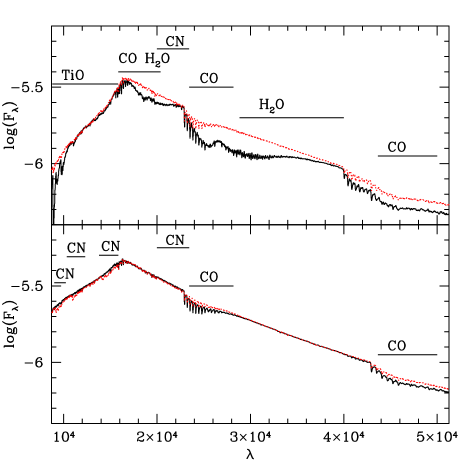
Figure 2: SED for P1 (solid lines) and P2 (dotted lines) [Fe/H]=$-$0.7 RGB models with $T_{\mathrm{e}ff}$=4052 K, $\log g$=1.12 (lower panel) and $T_{\mathrm{e}ff}$=3500 K, $\log g$=0.11 (upper panel). The vertical axis displays the logarithm of the flux in $erg/sec/cm{{}^{2}}/Hz/ster$, whilst the horizontal axis shows the wavelength in Å. The labels denote the main molecules contributing to the SED in those wavelength ranges where P1 and P2 results are different.

3 Colour- and pseudocolour-magnitude diagrams

A comparison of the BCs for P1 and P2 models provides the necessary guideline to assess whether NIRCam filters can identify the presence of multiple populations in massive clusters. Figures 3 and  4 display the difference between P1 and P2 models (P1-P2) at [Fe/H]=$-$0.7 and [Fe/H]=$-$1.62. Results for the case of [Fe/H]=$-$0.70 and $Y$=0.30 are within at most $\sim$0.01 mag of the results for [Fe/H]=$-$0.7 and normal $Y$.

In general, the differences of the BCs ($\Delta$(BC)) for all filters have a minimum around the main sequence turn off (located at log($g$)$\sim$4.0), and tend to increase moving along the RGB or going down along the main sequence. This is clearly due to a dependence of $\Delta$(BC) on $T_{\mathrm{e}ff}$, with $\Delta$(BC) increasing with decreasing $T_{\mathrm{e}ff}$ (see also Sbordone et al., 2011; Cassisi et al., 2013, for a similar result with Johnson-Cousins and Strömgren filters). The exact values of $\Delta$(BC) depend on the metallicity of the models, decreasing in absolute values when [Fe/H] decreases.

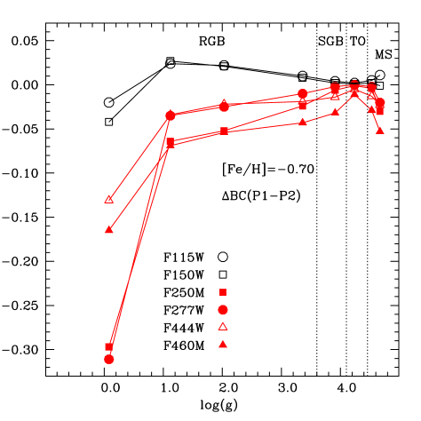
Figure 3: Difference ($\Delta$(BC)) between BCs calculated for P1 and P2 compositions (P1-P2), at selected points along a 12 Gyr isochrone with [Fe/H]=$-$0.7 and $Y$=0.256 (see Table 2). $\Delta$(BC) is plotted as a function of the surface gravity, that decreases steadily from the lower main sequence to the tip of the RGB. We also label the evolutionary phases –main sequence (MS), turn off (TO), subgiant branch (SGB) and RGB– corresponding to the selected isochrone points. Only filters showing the largest positive and negative differences are displayed (see text for details).

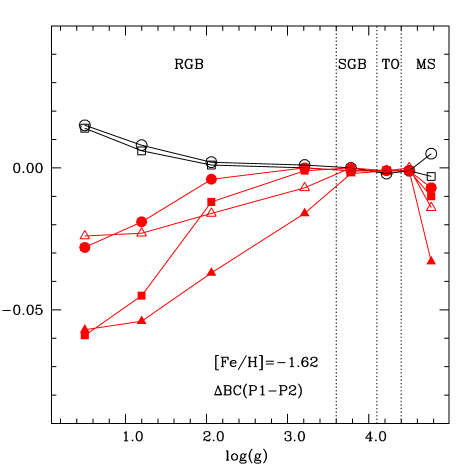
Figure 4: As Fig. 3 but for [Fe/H]=$-$1.62.

Focusing now on the RGB, the filters $F115W$ and $F150W$ show the largest positive $\Delta$(BC), whereas $F250M$, $F277W$, $F444W$ and $F460M$ display the largest negative variations. The narrow band filters $F466N$ and $F470N$ (not displayed in Figs. 3 and  4) follow exactly the same results as $F460M$. Notice that below $\sim$4000 K (log($g$)$\sim$1) at [Fe/H]=$-$0.7, $F250M$ and $F277W$ display a huge sudden decrease of $\Delta$(BC).

Figure 5 explains why the above-mentioned filters are the ones most affected by the P2 chemical composition. This figure shows the percentage difference of the SED between P1 and P2 models at the two coolest point along the [Fe/H]=$-$0.7 RGB, together with the passbands of the filters displayed in Fig. 3.

We consider first the spectra for $T_{\mathrm{e}ff}=$4052 K. SED differences are localized at specific wavelength ranges, and reflect the effect of the molecular abundances labelled in Fig. 2. The $F115W$ and $F150W$ filters are sensitive to variations of CN, that cause a decrease of the P2 flux compared to the P1 counterpart – the increase of N, much less abundant than C in the P1 composition, dominates over the decrease of C and causes an increase the strength of the CN molecular lines in the P2 SED– whereas $F250M$, $F277W$, $F444W$ and $F460M$ are sensitive to variations of CO, that increase the P2 flux compared to the P1 values (both C and O abundances in the P2 composition are decreased). This behaviour is typical of all SEDs along the RGB, apart from the coolest point at [Fe/H]=$-$0.7 ($T_{\mathrm{e}ff}=$3500 K).

Indeed, at $T_{\mathrm{e}ff}=$3500 K the situation is somewhat different, for in the wavelength range of $F115W$ and $F150W$ it is now the TiO absorption that starts to dominate. Due TiO variations $\Delta$(BC) values for these two filters change sign compared to higher $T_{\mathrm{e}ff}$ (see Fig. 3), but with values still close to zero.

For the $F444W$ and $F460M$ filters the CO absorption still dominates. In the wavelength regime of $F250M$ and $F277W$, the ${\rm H_{2}O}$ absorption becomes important above $\sim 26000$ Å, whilst between $\sim$22000 and $\sim$26000 Å  it is still mainly CO. Between $\sim$16000 and $\sim$22000 Å  variations of both CO and ${\rm H_{2}O}$ cause the observed flux differences, that were essentially zero at $T_{\mathrm{e}ff}=$4052 K. At [Fe/H]=$-$1.62 the RGB model $T_{\mathrm{e}ff}$ does never become low enough to see the effect on the BCs of TiO and ${\rm H_{2}O}$ variations.

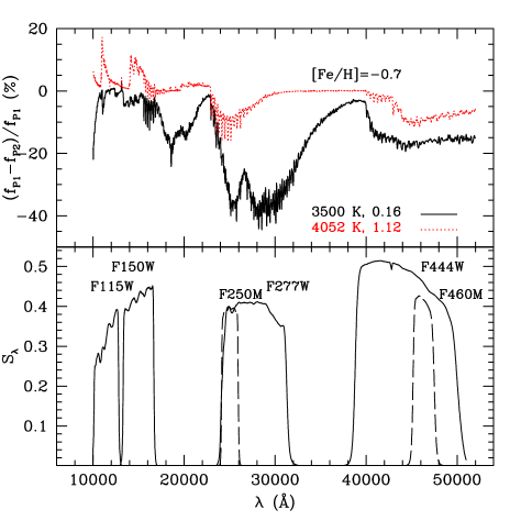
Figure 5: Upper panel: Percentage flux difference between the SED of P1 ($f_{P1}$) and P2 ($f_{P2}$) models with the labelled values of $T_{\mathrm{e}ff}$ and $\log g$, as a function of the wavelength $\lambda$ (in Å), in the range covered by the NIRcam filters discussed here. Lower panel: Total throughput of the wide and medium-band filters that cover the wavelength range showing the largest differences in the SED.

We emphasize here that these $\Delta$(BC) values are preserved also when calculated for younger RGB isochrones. Considering for example a 2 Gyr, [Fe/H]=$-$0.7 isochrone, for a given $T_{\mathrm{e}ff}$ on the RGB the surface gravity is changed by at most 0.1-0.2 dex compared to the $\log g$ values at the same $T_{\mathrm{e}ff}$ on a 12 Gyr isochrone. We have tested that these small changes of $\log g$ do not affect the $\Delta$(BC) results for the various NIRCam filters.

From the previous discussion we can conclude that colour-magnitude-diagrams (CMDs) like $M_{F150W}$-$(F150W-F460M)$, or $M_{F115W}$-$(F115W-F460M)$ shown in Fig. 6 – where we applied the calculated BCs to the reference 12 Gyr [Fe/H]=$-$0.7, $Y$=0.256 isochrone – can in principle reveal the presence of multiple populations along the cluster RGB. The P2 RGB is redder than the P1 counterpart, and the maximum colour separation with the chosen P2 pattern –that is at the upper limit of the observed range of abundance anticorrelations in Galactic GCs– is of about 0.10 mag along the upper RGB. At [Fe/H]=$-$1.62 this difference decreases by $\sim$0.01-0.02 mag. If the P2 composition has enhanced He ($Y$=0.30), the separation between P1 and P2 RGBs is reduced by $\leavevmode\nobreak\ \sim$0.01 mag.

It is possible in principle to consider also CMDs like $M_{F150W}$-$(F150W-F277W)$ and $M_{F150W}$-$(F150W-F250W)$ to maximize the separation of P1 and P2 only at magnitudes close to the RGB tip and at high metallicities (see results in Figs. 3 and  4).

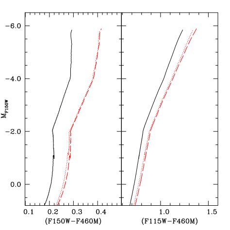
Figure 6: $M_{F150W}$-$(F150W-F460M)$ and $M_{F150W}$-$(F115W-F460M)$ diagram for 12 Gyr, [Fe/H]=$-$0.7, P1 (solid line) and P2 – with normal (dashed line) and enhanced (dotted line) initial He – isochrones.

To maximize the separation of P1 and P2 RGB tracks it is convenient to define – in a similar way as Milone et al. (2013), Piotto et al. (2015)– a pseudocolour, that is the difference of two colours that change with opposite signs when going from P1 to P2 composition. We have defined here the pseudocolour $C_{F150W,F460M,F115W}=(F150W-F460M)-(F460M-F115W)$, and we show in Fig. 7 the $M_{F150W}$-$C_{F150W,F460M,F115W}$ diagram for the same [Fe/H]=$-$0.7 isochrones of Fig. 6. The separation in $C_{F150W,F460M,F115W}$ between P1 and P2 isochrones is of the order of $\sim$0.1 mag along the lower RGB, increasing to $\sim$0.2 mag along the upper RGB, with a very small decrease if the P2 composition is He-enhanced. At [Fe/H]=$-$1.62 these figures are decreased by about 0.02-0.03 mag.

The alternative pseudocolour $C_{F150W,F277W,F115W}=(F150W-F277W)-(F277W-F115W)$ would enhance the separation of P1 and P2 RGBs compared to $C_{F150W,F460M,F115W}$, with differences up to $\sim$0.5 mag, but from only about 1 mag below the RGB tip in $M_{F150W}$, and for metal rich compositions.

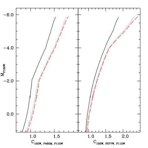
Figure 7: As Fig. 6 but for the $M_{F150W}$-$C_{F150W,F460M,F115W}$ and $M_{F150W}$-$C_{F150W,F277W,F115W}$ diagrams.

The effect of extinction in these photometric bands is, not suprisingly, small. We have determined the extinction relationships $A_{\lambda}/A_{V}$ for what we considered to be the best choice $F115W$, $F150W$ and $F460M$ filters discussed here, employing Cardelli et al. (1989) extinction law with $R_{V}=A_{V}/E(B-V)$=3.1 and the formalism by Girardi et al. (2002). We found $A_{F115W}/A_{V}$=0.32, $A_{F150W}/A_{V}$=0.21 and $A_{F460M}/A_{V}$=0.05, implying for the reddening affecting the pseudocolour $C_{F150W,F460M,F115W}$ a relationship $E(C_{F150W,F460M,F115W})=0.43A_{V}$. If we consider the pseudocolour $C_{F150W,F277W,F115W}$ , we find that $A_{F277W}/A_{V}$=0.09 and $E(C_{F150W,F277W,F115W})=0.35A_{V}$. To consider the case of extragalactic extinction laws with $R_{V}$ different from 3.1, we assumed $R_{V}$=5 as an example. We found in this case $A_{F115W}/A_{V}$=0.38, $A_{F150W}/A_{V}$=0.25, $A_{F460M}/A_{V}$=0.05, $A_{F277W}/A_{V}$=0.10, $E(C_{F150W,F460M,F115W})=0.53A_{V}$ and $E(C_{F150W,F277W,F115W})=0.43A_{V}$, values that are only marginally different from the results for $R_{V}=3.1$.

4 Discussion

In this paper we have studied the effect of MP chemical patterns on synthetic magnitudes in the JWST NIRCam filter system, identifying colours and pseudocolours able to disentangle MPs among clusters’ RGB stars. We found that colours like $(F150W-F460M)$ and $(F115W-F460M)$, or the pseudocolour $C_{F150W,F460M,F115W}$ are well suited to separate MPs over a reasonably large RGB temperature range, due to their sensitivity to variations of CN, CO and, with increasing metallicity, also TiO and ${\rm H_{2}O}$ molecular abundances.

With P2 light element abundance spreads typical of the extreme patterns observed in Galactic GCs, $C_{F150W,F460M,F115W}$ is predicted to display at [Fe/H]=$-$0.7 a range (at fixed luminosity) of the order of $\sim$0.1 mag along the lower RGB, increasing to $\sim$0.2 mag along the upper RGB. In case of the $(F150W-F460M)$ and $(F115W-F460M)$ colours, the expected range is of about 0.10 mag along the upper RGB. At a lower [Fe/H]=$-$1.62 these figures are reduced by 0.02-0.03 mag. Smaller MP abundance anticorrelations’ ranges will of course cause smaller colour and pseudocolour spreads, and the detection of MPs in extragalactic clusters using NIRCAM filters will depend on the actual photometric errors plus the range of cluster abundance anticorrelations in the target cluster, and the cluster [Fe/H].

It is interesting and useful to have a general idea of the maximum distance out to which it will be possible to disentangle MPs with JWST, at least for clusters with sizable abundance spreads. In the following experiment we require 0.01 mag photometric errors down to a couple of magnitudes below the RGB tip in the relevant NIRCAM filters. These photometric errors would enable us to definitely disentangle MPs in clusters at both [Fe/H]=$-$1.6 and $-$0.7, with CNONa abundance variations even lower than the maximum amplitudes observed in Galactic GCs.

We made use of the on-line JWST simulator for the NIRCam detector, and considered a RGB star of spectral type K0III –taken as representative of bright GC RGB objects– using the corresponding SED from the Phoenix stellar model atmosphere library (Husser et al., 2013). As a reasonable exposure time, we employed a set of 5 exposures, each one by 3 integrations, that are obtained with 8 groups (for a total of 15 integrations and total exposure time of about 24000 s).

To simulate the blending effects, we computed the average separation of RGB stars located at a distance $>1.7$ arcmin from the centre of the GC 47 Tuc - taken as representative of a typical crowding condition among GCs. We reported this separation to different distances, and for each distance we determined the corresponding angular separation, denoted by $s$. We considered then two representative RGB stars separated by $s$, and performed aperture photometry with radius $s$. We calculated the S/N of a single RGB star, considering the worst case that 50 % of the flux of the neighbouring object falls within the aperture.

With these assumptions, we found that at a distance of $\sim$1.4 Mpc (beyond the Andromeda Group, see, e.g., Karachentsev, 2005) we can still achieve the required 0.01 mag photometric error down to $\sim$2 mag below the RGB tip in the filters $F115W$, $F150W$ and $F460M$.

The F460M filter, that has a narrower passband compared to $F115W$ and $F150W$, does essentially set this distance for a fixed photometric error. We could in principle use the wider $F444W$ filter that is sensitive to the same molecular features as $F460M$ (see Figs. 2 and 5), but the price to pay is a reduction of the predicted sensitivity to MPs of the corresponding colours (see Figs. 3 and  4). By employing the pseudocolour based on $F277W$ ($C_{F150W,F277W,F115W}$, see Fig. 7) we would be able to disentangle MPs with a better or comparable sensitivity only down to $\sim$1 mag below the RGB tip. Nevertheless, with these alternative filter combinations and the same observational setup, the JWST simulator suggests that we could achieve 0.01 mag photometric errors two magnitudes below the RGB tip in all photometric filters at a distance of $\sim$5 Mpc (roughly the distance to the M83 Group and the Canes Venatici I Cloud, see e.g., Karachentsev, 2005).

To maximize the distance with the preferred colour/pseudocolour combinations involving the filter $F460M$, we studied an extreme case for a set of 10 exposures, each one by 5 integrations, obtained with 8 groups (total exposure time $\sim$ 80000 s). In this case we can achieve a 0.01 mag photometric error down to $\sim$2 mag below the RGB tip at a distance of $\sim$2.3 Mpc.

The standardization of real JWST data no doubt will turn out to be to some degree different from what we have employed in this analysis. Still, these results make it possible to obtain a first estimate of the appearance of MPs through the eye of JWST, and to assist with the planning of future observations when the telescope will be operational.