A Universality Theorem for Nested Polytopes

Abstract

In a nutshell, we show that polynomials and nested polytopes are topological, algebraic and algorithmically equivalent.

Given two polytops $A\subseteq B$ and a number $k$, the Nested Polytope Problem (NPP) asks, if there exists a polytope $X$ on $k$ vertices such that $A\subseteq X\subseteq B$. The polytope $A$ is given by a set of vertices and the polytope $B$ is given by the defining hyperplanes. We show a universality theorem for Nested Polytope Problem. Given an instance $I$ of the NPP, we define the solutions set of $I$ as

$$V^{\prime}(I)=\{(x_{1},\ldots,x_{k})\in\mathbb{R}^{k\cdot n}:A\subseteq\textrm{conv}(x_{1},\ldots,x_{k})\subseteq B\}.$$

As there are many symmetries, induced by permutations of the vertices, we will consider the normalized solution space $V(I)$.

Let $F$ be a finite set of polynomials, with bounded solution space. Then there is an instance $I$ of the NPP, which has a rationally-equivalent normalized solution space $V(I)$.

Two sets $V$ and $W$ are rationally equivalent if there exists a homeomorphism $f:V\rightarrow W$ such that both $f$ and $f^{-1}$ are given by rational functions. A function $f:V\rightarrow W$ is a homeomorphism, if it is continuous, invertible and its inverse is continuous as well.

As a corollary, we show that NPP is $\exists\mathbb{R}$-complete. This implies that unless $\exists\mathbb{R}=\mbox{NP}$, the NPP is not contained in the complexity class NP. Note that those results already follow from a recent paper by Shitov [34]. Our proof is geometric and arguably easier.

1 Introduction

Definition.

In the Nested Polytope Problem (NPP), we are given two polytopes $A\subseteq B\subset\mathbb{R}^{n}$ and a number $k\in\mathbb{N}$ and we ask, whether there exists a polytope $A\subseteq X\subseteq B$ with $k$ vertices. To be more precise the inner polytope $A$ is specified by its vertices and the outer polytope $B$ is specified by its facets. Given an instance $I=(A,B,k)$, we denote by

$$V^{\prime}(I)=\{(x_{1},\ldots,x_{k})\in\mathbb{R}^{k\cdot n}:A\subseteq\textrm{conv}(x_{1},\ldots,x_{k})\subseteq B\}.$$

the set of solutions. Here $\textrm{conv}(x_{1},\ldots,x_{k})$ denotes the convex hull of the points $x_{1},\ldots,x_{k}$. Given a permutation $\pi:[k]\rightarrow[k]$, we can for every solution $x\in V^{\prime}(I)$ get a new solution denoted by $x_{\pi}$. Note that $V^{\prime}(I)$ has a lot of symmetries as every permutation of the vertices of a valid solution yields again a valid solution. We say two solutions $x,y$ are permutation-equivalent if there exists a permutation $\pi$ of the vertices, so that $x_{\pi}=y$. We denote this by $x\sim y$. We define the normalized solution space by

$$V(I)=V^{\prime}(I)/\sim.$$

It is not a priori clear that $V(I)$ can be interpreted as a subset of $\mathbb{R}^{kn}$. And for some instances $I$, this will not be the case. However, for the instances that we produce it is. For us every instance $I$ has a set $S$ of $k$ disjoint segments associated to it. We will show that on each segment must lie exactly one vertex in any valid solution. Let $\prec$ be an order on $S$. Then we can think of $V(I)$ simply as the vertices of the intermediate polytope given in the order $\prec$ and thus $V(I)\subset\mathbb{R}^{kn}$.

Rational-Equivalence.

On a very high-level, a universality theorem states that we can represent any objects of type $A$ by an object of type $B$ preserving property $C$. In our case, objects of type $A$ are just bounded algebraic varietes, which we will formally define below. They are very versatile as they can encode many different mathematical objects of interest in a straight-forward fashion. Instances of the NPP are the objects of type $B$. At last, we want to preserve algebraic and topological properties. In this paragraph, we define the notion of rational-equivalence, which preserve both [34].

Let $F$ be a finite set of polynomials $F=\{f_{1},\ldots,f_{k}\}$ with $f_{i}\in\mathbb{Z}[x_{1},\ldots,x_{n}],\,i=1,\ldots,k$. Then we define the variety of $F$ as

$$V(F)=\{x\in\mathbb{R}^{n}:f(x)=0,\ \forall f\in F\}.$$

We say $V(F)$ is bounded, if there is a ball $B$ such that $V(F)\subseteq B$.

Two varieties $V$ and $W$ are rationally equivalent if there exists a homeomorphism $f:V\rightarrow W$ such that both $f$ and $f^{-1}$ are given by rational functions. A function $f:V\rightarrow W$ is a homeomorphism, if it is continuous, invertible and its inverse is continuous as well. The function $f$ is rational, if it can be component-wise described as the ratio of polynomials. We denote rational-equivalence by $V\simeq W$. Note that the composition of two homeomorphisms is a homeomorphism. Similarly, the composition of two rational functions is rational. Next to algebraic and topological properties, we preserve also algorithmic properties. To state this properly, we will introduce the complexity class $\exists\mathbb{R}$ in the next paragraph.

Existential Theory of the Reals.

In the study of geometric problems, the complexity class $\exists\mathbb{R}$ plays a crucial role, connecting purely geometric problems and Real Algebraic Geometry. Whereas NP is defined in terms of existentially quantified Boolean variables, $\exists\mathbb{R}$ deals with existentially quantified real variables.

Consider a first-order formula over the reals that contains only existential quantifiers,

$$\exists x_{1},x_{2},\ldots,x_{n}:\Phi(x_{1},x_{2},\ldots,x_{n}),$$

where $x_{1},x_{2},\ldots,x_{n}$ are real-valued variables and $\Phi$ is a quantifier-free formula involving equalities and inequalities of integer polynomials. The algorithmic problem Existential Theory of the Reals (ETR) takes such a formula as an input and asks whether it is satisfiable. The complexity class $\exists\mathbb{R}$ consists of all problems that reduce in polynomial time to ETR. Many problems in combinatorial geometry and geometric graph representation naturally lie in this class, and furthermore, many have been shown to be $\exists\mathbb{R}$-complete, e.g., stretchability of a pseudoline arrangement [25, 27, 33], recognition of segment intersection graphs [23] and disk intersection graphs [26], computing the rectilinear crossing number of a graph [5], etc. For surveys on $\exists\mathbb{R}$, see [32, 9, 25]. A recent proof that the Art Gallery Problem is $\exists\mathbb{R}$-complete [1] provides the framework we follow in our proof. See also [6, 36, 9, 33, 32, 25, 20, 24, 26, 31, 11, 10] for a small selection of $\exists\mathbb{R}$-complete problems.

Results.

We show a universality theorem for the NPP. Note that the result is implied by a recent result of Shitov [34] about Non-negative Matrix Factorization and an old reduction due to Cohen and Rotblum [14]. Thus we attribute the result to Shitov.

Theorem 1 (Universality Shitov [34].).

For every bounded variety $V(F)$ exists an instances $I$ of the Nested Polytope Problem such that $V(I)\simeq V(F)$.

In this paper, we give a direct proof that does not use either of the two above papers. The main ideas of our proof are simple geometric constructions. This implies that polynomial equations have a solution space that is topologically and algebraically equivalent to solution spaces given by the NPP. To illustrate the strength of the statement, we highlight give one algebraic corollary and one topological example.

Corollary 2 (Algebraic Consequences).

Let $\mathbb{Q}\subseteq F_{1}\subset F_{2}\subset\mathbb{R}$ be two algebraic field extensions of $\mathbb{Q}$. Then there exists an instance of the NPP such that there is a solution in $F_{2}$, but not in $F_{1}$.

This implies for instance the result by [12], who showed that there is an instance of the Nested Polytope Problem that requires irrational coordinates.

Example 3 (Topological Consequences).

Let $T$ be a torus, then there is an instance of the NPP such that the solution space is homeomorphic to $T$.

Note that the polynomial equation

$$f(x,y,z)=(x^{2}+y^{2}+z^{2}+R^{2}-r^{2})^{2}-4R^{2}(x^{2}+y^{2})=0$$

describes a torus with the two radii $r$ and $R$. To see the last corollary, simply apply Theorem 1 on the variety given by $f$, with $R=10,r=1$.

As all the steps involved to show this universality theorem take polynomial time to execute we can infer the algorithmic complexity of the NPP.

Corollary 4 (Shitov [34]).

The Nested Polytope Problem is $\exists\mathbb{R}$-complete.

In the rest of the introduction, we survey the literature on the NPP and the closely related problem of Non-negative Matrix Factorization.

Proof Overview.

The proof consists of two parts. In Section 2, we show that a certain very simple set of polynomial equations is already $\exists\mathbb{R}$-complete and admits the desired universality property. In a nutshell, we only allow only the constraints $x\cdot y=1$ and $x+y+z=5/2$.

In the second part, in Section 3, we are encoding those constraints in the NPP. The first idea is to enforce certain vertices to lie on specific line segments. Those vertices are encoding variables. It is very easy to build polytopes that encode the two constraints explained above. The main technical challenge is to ”stick” those smaller building blocks together to a ”big one”. This is easy, if you are used to work with polytopes in higher dimensions. In our description, we do not assume the reader to have that familiarity. See also Figure 1

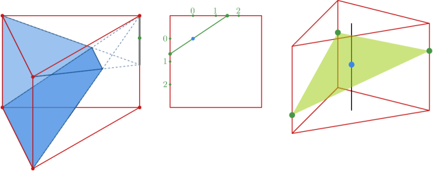
Figure 1: Red indicates the outer polytope, blue the inner polytope, and green the nested polytope. Left: The nested polytope must have one vertex on the left bottom edge. Middle: Assuming that one nested vertex is on the left edge and one at the top edge, then the two vertices encode inversion. Right: Assuming that each green vertex is forced to be on its vertical segment, then the blue vertex enforces the constraint $x+y+z=5/2$.

Related Work on Nested Polytopes.

To the best of our knowledge the NPP was first mentioned by Silio in 1979 [37], who could find an $O(nm)$ time algorithm in the case that the outer and inner polytope are convex polygons in the plane with $n$ and $m$ vertices respectively. Additionally, Silio restricts to the case $k=3$. The motivation of Silio came from a connection to Stochastic Sequential Machines.

Independently, Victor Klee suggested the same problem as was pointed out in several papers [17, 2, 15, 30, 16], the first of them dating back to 1985. In particular, the NPP appears as one of the open problem in the Computational Geometry Column $\#4$ [30]. The main motivation of those early papers used to be simplification of a given polytope, see Figure 2.

Figure 2: Using an algorithm for the nested polygon problem it is possible to attain a simplified version of the previous polygon.

Among the first results is an $O(n\log k)$ algorithm for the nested convex polygon problem [2]. On the lower bounds side, Das and Joseph showed NP-hardness for the NPP in dimension three [17, 15, 18, 16].

In 1995, Suri and Mitchell were able to reduce the NPP to a set cover problem, by loosing only a factor of $d$. Their motivation to study the NPP came from separating geometric objects. Using the greedy approximation scheme for set cover they attain an $O(d\log n)$-approximation algorithm that runs in $O(n^{d+1})$ time ($n=$ number of facets of inner and outer polytope, $d=$ dimension). This was consequently improved by Brönnimann and Goodrich [7] as the first application in their seminal paper on $\varepsilon$-nets. The key observation is that the set-cover system described by Suri and Mitchell has bounded VC-dimension. Their algorithm runs in $O(n^{d+2}\log^{d}n)$ and gives an $O(d^{2}\log OPT)$-approximation ($OPT=$ size of the optimal solution) . Independently Clarkson [13] found a similar approximation algorithm using techniques from linear programming.

Interestingly, the NPP has close relations to Non-negative Matrix Factorization. We define NMF, explain the history and this relation in the next paragraph.

Non-Negative Matrix Factorization.

In a parallel line of research the NMF is explored, with the earliest mentioning, we found, in 1973 [4]. The non-negative matrix factorization is defined as follows. Given a matrix $M\in\mathbb{R}_{+}^{m\times n}$ and a number $k$, we say that $M=V\cdot W$, for matrices $V\in\mathbb{R}_{+}^{m\times k}$ and $W\in\mathbb{R}_{+}^{k\times n}$, is a non-negative matrix factorization of inner dimension $k$. We denote by $\mathbb{R}_{+}$ the set of non-negative real numbers. We denote by $\textrm{rank}_{+}(M)$ the non-negative rank, which is the smallest inner dimension, for which a non-negative matrix factorization exists.

While it is said that NMF has many applications in image processing, machine learning, dimension reduction and clustering, in theory it is most famous for the relationship to extension complexity. Given a polytope $P$, its extension complexity, is the smallest number $k$ such that there is a polytope $Q$ on $k$ facets such that there is a linear projection from $Q$ to $P$. Yannakakis showed in its seminal paper [41] (Roughly saying that on needs an exponential size symmetric LP to solve the travelling salesperson problem.) that the extension complexity of a polytope is the non-negative rank of its slack matrix. See also [21] for the lower bound for non-symmetric LPs.

For us most relevant is a reduction from the NMF to NPP by Cohen and Rothblum [14]. To the delight of the reader, we repeat this reduction in the appendix.

Lemma A (Cohen Rothblum [14]).

Let $M\in\mathbb{R}^{m\times n}_{+}$ be a matrix and $k\in\mathbb{N}$ be a number. Let $A$ be the convex hull intersected with $H=\{x\in\mathbb{R}^{m}:\sum_{i}x_{i}=1\}$ and $B$ the positive orthant intersected with $H$. Then $(A,B,k)$ as an instance to the NPP is equivalent to $(M,k)$ as NMF.

In 2009, Vavasis [40] showed that exact-non-negative matrix factorization is equivalent to the intermediate simplex problem. In particular, their results imply that the NPP is already hard, if the intermediate polytope is restricted to be a simplex. In a similar way, Gillis and Glineur [22] in 2010 showed that restricted non-negative matrix factorization is equivalent to NPP.

Although, it is easy to encode NMF as an algebraic decision problem the huge number of variables makes it algorithmically infeasible. In 2012, Arora Ge, Kannan and Moitra [3] found an algorithm that runs in polynomial time for every fixed $k$. They also showed that there is no $(nm)^{o(k)}$, assuming ETH. In 2016 Moitra [28] improved the upper bound and gave an $(nm)^{O(k^{2})}$ algorithm for NMF. Note that those results translate immediately to results about NPP, due to the reductions mentioned above.

Chistikov, Kiefer, Marušić, Shirmohammadi, Worrell have shown that the optimal solution of the Nested Polytope Problem requires irrational coordinates already in dimension $d=3$ and $k=5$. It is an open problem, if the intermediate-simplex problem requires irrational coordinates as well. This was also shown in parallel by Shitov [35]. Furthermore, Shitov showed a universality result for NMF, very similar to our result. In particular, his result implies $\exists\mathbb{R}$-completeness of both NMF and the NPP.

2 Encoding ETR

In this section, we define the algorithmic problem and the complexity class both called the Exitential Theory of the Reals. For distinction, the algorithmic problem is denoted by ETR and the complexity class by $\exists\mathbb{R}$.

An instance of ETR is a well-formed logical formula of the form

$$\exists x_{1},\ldots,x_{n}:\phi(x_{1},\ldots,x_{n}).$$

The subformula $\phi$ is quantifier free. It has polynomial equations and (strict) inequalities as atomic formulas. Those atomic formulas can be combined in any boolean way. For example:

$$\exists x,y,z:[(x^{2}+y^{2}=1)\land(x=-2)]\lor\lnot(y^{2}z<-1).$$

Strictly speaking, we are only allowed to use variables and the symbols

$$\Sigma=\{+,\cdot,=,>,\leq,(,),0,1,\land,\lor,\lnot\}.$$

However, we interpret $x^{2}$ as $x\cdot x$ and $x=-2$ as $x+1+1=0$ and so on. We are asking if there is an assignment of real numbers to the variables such that the formula $\phi$ becomes true. Note that the definition in the introduction and the more precise definition here are equivalent, although this may not be obvious.

It is not a priory clear that there even exists an algorithm which can decide this problem. Due to Tarski’s Quantifier Elimination [38], we know that this question can be decided. Even more, we know that the problem can be solved in polynomial space, due to Canny [8]. The complexity class $\exists\mathbb{R}$ is defined as the set of algorithmic problems that can be reduced in polynomial time to ETR.

An ETR-INV-system $\mathcal{S}$ of size $n$ is a vector of $n$ real variables $(x_{1},\dots,x_{n})\in[\frac{1}{2},2]^{n}$ together with a system of linear and quadratic equations of the form

$$x+y=z\;\;\;,\;\;\;x\cdot y=1.$$

The solution space of an ETR-INV-system $\mathcal{S}$ is the set of all vectors in $[\frac{1}{2},2]^{n}\subset\mathbb{R}^{n}$ which satisfy the equations of $\mathcal{S}$, where we do allow the possibility of an empty solution space. (Note that the solution space of an ETR-INV-system is a real semi-algebraic set.) It was shown in [1, Lemma 12] that the problem of determining whether an ETR-INV-system has a non-empty solution space is $\exists\mathbb{R}$-complete. (The original formulation of ETR-INV-system included the equation $x=1$, but this equation can be obtained by $x\cdot x=1$ and $x\in[\frac{1}{2},2]$) Although, this was not pointed out directly, if we follow the reduction it is easy to observe that all steps are rationally-equivalent.

Lemma 5 (Universality Inversion).

Let $F$ be a finite set of polynomials $F=\{f_{1},\ldots,f_{k}\}\subset\mathbb{Z}[x_{1},\ldots,x_{n}]$, with bounded solution space. There is an instance $I$ of ETR-INV-system such that

$$V(I)\simeq V(F).$$

Proof Sketch..

In almost every step of the reduction a new variable and a new constraint is introduce. All other variables are left as they are. For example, $Y\cdot X_{i}-1=0$, where $X_{i}$ is an old variable and $Y$ is a new variable. Of course, there is the assumption that $X\not=0$. We see that $Y=1/X$, which determines that the new and the old system of equations are rationally equivalent. To be explicit, the following mapping

$$f:(x_{1},\ldots,x_{n})\mapsto(x_{1},\ldots,x_{n},1/x_{i}),$$

is a homeomorhpism, it is rational and its inverse is rational as well.

Note that there are two exceptions. The inequality $X>0$ is replaced by $XY^{2}-1=0$. Note that this step does not preserve homotopy as the two sets

$$S=\{x:x>0\}$$

and

$$T=\{(x,y):xy^{2}-1=0\}$$

do not have the same number of connected components. However, we restrict ourselves to systems of polynomial equations.

The second exception is when all variables are scaled down to a small range. Note that the sets

$$A=\{(x,y):x+y=1\}$$

and

$$B=\{(x,y):x+y=1,-L\leq x,y\leq L\}$$

are not rationally equivalent. But again, this does not apply to us, as we assume that the initial solution space is bounded. ∎

While ETR-INV-system is the right intermediate problem to show that the Art Gallery Problem is $\exists\mathbb{R}$-complete, for the purpose of this paper however, it will be more convenient to work with a slight modification of ETR-INV-system, which we introduce now.

An ETR-INV-array $\mathcal{A}$ of size $m\times n$ is an $m$-by-$n$ matrix of variables $A=(\alpha_{i,j})\in[\frac{1}{2},2]^{m\times n}$ together with a system of linear and quadratic equations of the form

$$\alpha_{i,j}+\alpha_{i,k}=\tfrac{5}{2}\;\;\;,\;\;\;\alpha_{i,j}+\alpha_{i,k}+\alpha_{i,l}=\tfrac{5}{2}\;\;\;,\;\;\;\alpha_{i,k}\cdot\alpha_{j,k}=1.$$

(Note that the linear equations relate variables in the same row and the quadratic equations relate variables in the same column.)

The solution space of an ETR-INV-array is defined similarly as for ETR-INV-system and is a semi-algebraic subset of $[\frac{1}{2},2]^{m\times n}\subset\mathbb{R}^{m\cdot n}$. We now have the following lemma.

Lemma 6 (Uninversality of ETR-INV-array).

Let $\mathcal{S}$ be an ETR-INV-system on $n$ variables. There exists an ETR-INV-array $\mathcal{A}$ of size $3\times 2n$ such that the solution spaces of $\mathcal{S}$ and $\mathcal{A}$ are rationally-equivalent. The description complexity of $\mathcal{A}$ is linear in $\mathcal{S}$.

Proof.

Let us denote by $x_{1},\ldots,x_{n}$ the variables of $\mathcal{S}$. First note that we can assume without loss of generality that every variable $x_{i}$ in $\mathcal{S}$ is in at most one inversion constraint involved. Otherwise $x\cdot y=1$ and $y\cdot z=1$, implies $x=z$ and we can replace $z$ everywhere by $x$ and forget about $z$. Note that this preserves rational equivalence.

We denote the variables of $\mathcal{A}$ by $y_{i},\alpha_{i},\beta_{i},\gamma_{i},\delta_{i},\varepsilon_{i}$, for $i=,\ldots,n$ and we write them into the array as follows

$$\left(\begin{array}[]{cc}y_{1}\ldots y_{n}&\alpha_{1}\ldots\alpha_{n}\\ \beta_{1}\ldots\beta_{n}&\gamma_{1}\ldots\gamma_{n}\\ \delta_{1}\ldots\delta_{n}&\varepsilon_{1}\ldots\varepsilon_{n}\end{array}\right).$$

We want that all constraints in $\mathcal{S}$ for the $x_{i}$ variables hold in $\mathcal{A}$ for the corresponding $y_{i}$ variables. The remaining variables in $\mathcal{A}$ are supposed to be completely determined. We introduce the linear constraint

$$y_{i}+\alpha_{i}=5/2,$$

for every $i=1,\ldots,n$. Let us first consider linear constraints of the form

$$x_{i}+x_{j}=x_{k},$$

in $\mathcal{S}$. We introduce the linear constraint,

$$y_{i}+y_{j}+\alpha_{k}=5/2.$$

Note that this implies

$$y_{i}+y_{j}=y_{k}.$$

This encodes all linear constraints. Now let us consider the quadratic constraints, involving two different variables. Note that we denote the pairs of constraints as

$$C=\{(i,j):i<j,\,x_{i}\cdot x_{j}=1\}.$$

For every $(i,j)\in C$, we are adding the constraints

$$y_{i}\cdot\beta_{i}=1\text{ and }\beta_{i}\cdot\delta_{i}=1.$$

Similarly, we add the constraints

$$y_{j}\cdot\delta_{j}=1\text{ and }\beta_{j}\cdot\delta_{j}=1.$$

This enforces $\beta_{i}=1/y_{i}$ and $\beta_{j}=y_{j}$. Furthermore, we add the constraints

$$\beta_{i}+\gamma_{i}=5/2,\text{ and }\beta_{j}+\gamma_{i}=5/2,$$

This enforces $1/y_{i}=\beta_{i}=\beta_{j}=y_{j}$, as desired.

Let us now consider the special case of $x_{i}\cdot x_{i}=1$. Recall that this is equivalent to $x_{i}=1$. We introduce the constraints

$$y_{i}\cdot\beta_{i}=1,\ \beta_{i}\cdot\delta_{i}=1,\text{ and }y_{i}\cdot\delta_{i}=1.$$

This is equivalent to $y_{i}=1$.

Note that all the $\varepsilon_{i}$’s variables and some of the $\beta_{i},\gamma_{i},\delta_{i}$ variables are still completely unconstrained. Add any linear constraint of the form $a+b=5/2$ with an already used variable to them, so that they are uniquely determined, by one of the $y_{i}$. We have that the set of constraints on the $x_{i}$’s and one the $y_{i}$’s are exactly the same.

Let use denote by $V=V(\mathcal{S})$ the solution space of $\mathcal{S}$ and by $W=V(\mathcal{A})$ the solution space of $\mathcal{A}$. We have to show that $V$ and $W$ are rationally-equivalent. To this end we define the mapping

$$f:V\rightarrow W.$$

Let $(x_{1},\ldots,x_{n})$ in $V$. Then we define $y_{i}:=x_{i}$. We define $\alpha_{i}:=5/2-x_{i}$. Each $\beta_{i}$ and $\delta_{i}$ is either $x_{i}$ or $1/x_{i}$, if the index $i$ was contained in a pair in $C$. All other variables $\theta$ are of the form $5/2-x_{j}$ or $5/2-1/x_{j}$, for some $j$. Note that $f$ is bijective, as the set of constraints onto the $x_{i}$’s and $y_{i}$’s are the same. The mapping $f$ is continuous and rational by definition. The inverse mapping $f^{-1}:W\rightarrow V$ is simply given by

$$\left(\begin{array}[]{cc}y_{1}\ldots y_{n}&\alpha_{1}\ldots\alpha_{n}\\ \beta_{1}\ldots\beta_{n}&\gamma_{1}\ldots\gamma_{n}\\ \delta_{1}\ldots\delta_{n}&\varepsilon_{1}\ldots\varepsilon_{n}\end{array}\right)\mapsto(y_{1},\ldots,y_{n}).$$

This is also a continuous and rational mapping. Note that the number of constraints and variables of $\mathcal{A}$ is linear in the number of variables and constraints of $\mathcal{S}$. This finishes the proof. ∎

3 Building the polytopes

The main goal of this section is to prove the following lemma.

Lemma 7.

Let $\mathcal{A}$ be an ETR-INV-array of size $m\times n$. There exists convex polytopes $A\subset B\subset\mathbb{R}^{2+n+m}$ such that there exists a nested polytope $A\subset X\subset B$ with $k=mn+2m+2$ vertices such that the solution spaces are rationally-equivalent.

Remark 8.

The polytopes $A\subset B$ in Lemma 7 are actually contained in a hyperplane in $\mathbb{R}^{2+n+m}$, and are $(n+m+1)$-dimensional. The outer polytope $B$ will have $(n+2)(m+1)$ vertices and is defined by $n+m+3$ hyperplanes. The vertex description and facet description of the outer polytope will be given in Subsection 3.3.1.

The inner polytope $A$ has $2m+2$ vertices in common with the outer polytope $B$ together with an additional $2mn$ vertices that lie on certain 2-faces of the outer polytope. Finally, for each equation in the ETR-INV-array $\mathcal{A}$ we add one additional vertex to the inner polytope which will lie on certain faces of the outer polytope. The vertex description of the inner polytope $A$ is given in Subsection 3.3.2.

3.1 Two geometric observations

Here we state two simple geometric observations that are used for the “gadgets” needed in our construction of the polytopes of Lemma 7.

3.1.1 The linear equations

Let $\{v_{0},v_{1},\dots,v_{k}\}$ be a set of affinely independent points in $\mathbb{R}^{d}$. For $1\leq i\leq k$ let $w_{i}=v_{i}+v_{0}$ and define the prism $P$ as

$$P=\textrm{conv}(\{v_{1},\dots,v_{k},w_{1},\dots,w_{k}\}).$$

For $t\in[0,1]$ define the point $q_{t}\in P$ as

$$q_{t}=(1-t)(\tfrac{1}{k}v_{1}+\cdots+\tfrac{1}{k}v_{k})+t(\tfrac{1}{k}w_{1}+\cdots+\tfrac{1}{k}w_{k})=\tfrac{1}{k}v_{1}+\cdots+\tfrac{1}{k}v_{k}+tv_{0}.$$

Finally, for $1\leq i\leq k$ define points $p_{i}$ as

$$p_{i}=(1-\lambda_{i})v_{i}+\lambda_{i}w_{i}=v_{i}+\lambda_{i}v_{0},$$

where $\lambda_{i}\in[0,1]$. A simple calculation (left to the reader) gives us the following.

Observation 9.

$q_{t}\in\textrm{conv}(\{p_{1},\dots,p_{k}\})$ if and only if $\sum_{i=1}^{k}\lambda_{i}=tk$.

3.1.2 The quadratic equation

In the plane $\mathbb{R}^{2}$, let $p_{1}=(\alpha_{1},-1)$ be a point on the line $y=-1$ and let $p_{2}=(-1,\alpha_{2})$ be a point on the line $x=-1$, where $\alpha_{1},\alpha_{2}\in[\frac{1}{2},2]$. A simple calculation (left to the reader) gives us the following.

Observation 10.

The origin $(0,0)\in\textrm{conv}(\{p_{1},p_{2}\})$ if and only if $\alpha_{1}\cdot\alpha_{2}=1$.

3.2 A basic outline of the construction

We now give an outline of the construction of the polytopes in Lemma 7, without giving explicit coordinates, but rather focusing on the three “gadgets” that will be used to encode the three types of equations in $\mathcal{A}$. (We will give precise coordinates in Subsection 3.3.)

3.2.1 The outer polytope

To build the outer polytope $B$ we start with an “orthogonal frame” spanning $\mathbb{R}^{m}$, consisting of $m$ mutually orthogonal segments of equal length all meeting in a common endpoint. Note that the convex hull of these segments form an $m$-dimensional simplex. (When we eventually add coordinates, the length of these segments will be 3 units, each one parametrizing the closed interval $[-1,2]$.) We now take $n+2$ distinct copies of the orthogonal frame, $U_{1}$, $U_{2}$, $V_{1},\dots,V_{n}$, each one translated into “independent dimensions” so that their union now lives in $\mathbb{R}^{2+n+m}$ (Note that the affine span of the union will be $(n+m+1)$-dimensional.) We label the segments of these orthogonal frames as

$$\begin{array}[]{ccc}U_{1}&=&\{\tau_{1,1},\dots,\tau_{m,1}\}\\ U_{2}&=&\{\tau_{1,2},\dots,\tau_{m,2}\}\\ V_{1}&=&\{\sigma_{1,1},\dots,\sigma_{m,1}\}\\ &\vdots&\\ V_{n}&=&\{\sigma_{1,n},\dots,\sigma_{m,n}\}\end{array}$$

such that the segments $\tau_{i,1},\tau_{i,2},\sigma_{i,1},\dots,\sigma_{i,n}$ are all parallel.

We now take the outer polytope $B$ to be the convex hull of $U_{1}\cup U_{2}\cup V_{1}\cup\cdots\cup V_{n}$. It is straight-forward to show that $B$ is an $n+m+1$-dimensional polytope with $(n+2)(m+1)$ vertices. In what follows, for each $1\leq i\leq m$ and $1\leq j\leq n$, the “second half” of segment $\sigma_{i,j}$, parametrizing the interval $[\frac{1}{2},2]$, will correspond to the variable $\alpha_{i,j}$ in the ETR-INV-array $\mathcal{A}$. The segments $\tau_{i,j}$ will play an auxiliary role which we describe next.

3.2.2 Building the inner polytope: Enforcing vertices to segments

The first step in building the inner polytope $A$ is to enforce the following.

Property 11.

Let $X$ be a nested polytope, with $k=mn+2m+2$ vertices and $A\subset X\subset B$. For every $1\leq i\leq m$ and $1\leq j\leq n$, the segment $\sigma_{i,j}\in V_{j}$ contains exactly one vertex of $X$, which we denote by $x_{i,j}$.

(More specifically, each segment of the orthogonal frame $V_{i}$ will contain exactly one vertex from $X$ in its “second half”, thus encoding a value in the interval $[\frac{1}{2},2]$.) This can be done as follows. Fix indices $1\leq i\leq m$ and $1\leq j\leq n$, and consider segment $\tau_{i,1}\in U_{1}$ and its parallel copy $\sigma_{i,j}\in V_{j}$, which are edges of a $2$-dimensional face of the outer polytope $B$. Define the point $y_{i,j}$ to be the unique point in this 2-face such that segment $\tau_{i,1}\in U_{1}$ is mapped to the second half of its parallel copy $\sigma_{i,j}\in V_{j}$ by central projection through $y_{i,j}$. Similarly, we define the analogous point $z_{i,j}$ in the $2$-face of $A$ spanned by the segment $\tau_{i,2}\in U_{2}$ and its parallel copy $\sigma_{i,j}\in V_{j}$. (See Figure 3.)

Figure 3: The vertices of any nested polytope $A\subset X\subset B$ (marked in red) must include the endpoints of segments $\tau_{i,1}\in U_{1}$ and $\tau_{i,2}\in U_{2}$, while the last vertex, $x_{i,j}$, must be contained in the segment $\sigma_{i,j}\in V_{j}$ restricted to the interval $[\frac{1}{2},2]$.

At this stage of the construction the inner polytope $A$ will consist of the orthogonal frames $U_{1}$ and $U_{2}$ together with the points $\{y_{i,j},z_{i,j}\}$ for all $1\leq i\leq m$ and $1\leq j\leq n$. Moreover, if $X$ is a nested polytope, with $mn+2m+2$ vertices and $A\subset X\subset B$, then $X$ must contain the orthogonal frames $U_{1}$ and $U_{2}$. This accounts for $2m+2$ of the vertices, as all $\tau_{i,1}$ (the same for the $\tau_{i,2}$.) have one end point in common. Futermore, $X$ must contain one vertex in each of the segments of the orthogonal frames $V_{1},\dots,V_{n}$. This accounts for the remaining $m\cdot n$ vertices. Thus Property 11 is satisfied, and we let $x_{i,j}$ denote the unique vertex of $X$ which is contained in the (second half of the) segment $\sigma_{i,j}\in V_{j}$, which we associate with the variable $\alpha_{i,j}\in[\frac{1}{2},2]$.

3.2.3 Building the inner polytope: Encoding $\alpha_{i,j}+\alpha_{i,k}=\frac{5}{2}$

In order to enforce the relation $\alpha_{i,j}+\alpha_{i,k}=\frac{5}{2}$, we add a new vertex $p_{i,j,k}$ to the inner polytope $A$ as follows. We consider the rectangular 2-face of the outer polytope $B$ spannced by the segements $\sigma_{i,j}\in V_{j}$ and $\sigma_{i,k}\in V_{k}$. Define $p_{i,j,k}$ to be the point in this 2-face such that $p_{i,j,k}$ is contained in the convex hull of the vertices $x_{i,j}$ and $x_{i,k}$ of the nested polytope $X$ (satisfying Property 11) if and only if the associated variables $\alpha_{i,j}+\alpha_{i,k}=\frac{5}{2}$. (The unique point $p_{i,j,k}$ exists by Observation 9 by letting $\{v_{1},w_{1}\}$ be the endpoints of $\sigma_{i,j}$ and $\{v_{2},w_{2}\}$ be the endpoints of $\sigma_{i,k}$. See Figure 4.)

Figure 4: The vertices $x_{i,j}$ and $x_{i,k}$ contain the point $p_{i,j,k}$ in their convex hull if and only if the associated variables satisfy the equation $\alpha_{i,j}+\alpha_{i,k}=\frac{5}{2}$

Let us now add the vertex $p_{i,j,k}$ to $A$, and consider a nested polytope $X$ satisfying Property 11. It is easily shown that the only possible way that $X$ can contain the point $p_{i,j,k}$, is if this point is contained in $\textrm{conv}(\{x_{i,j},x_{i,k}\})$. In other words, if $X$ satisfies Property 11, then the associated variables satisfy the equation $\alpha_{i,j}+\alpha_{i,k}=\frac{5}{2}$.

3.2.4 Building the inner polytope: Encoding $\alpha_{i,j}+\alpha_{i,k}+\alpha_{i,l}=\frac{5}{2}$

Enforcing the relation $\alpha_{i,j}+\alpha_{i,k}+\alpha_{i,l}=\frac{5}{2}$ is similar to the previous case, and we add a new vertex $q_{i,j,k,l}$ to the inner polytope $A$ as follows. We consider the triangluar prism spanned by the segments $\sigma_{i,j}\in V_{j}$, $\sigma_{i,k}\in V_{k}$, and $\sigma_{i,l}\in V_{l}$, which is a 3-face of the outer polytope $B$.

Define $q_{i,j,k,l}$ to be the point in this 3-face such that $q_{i,j,k,l}$ is contained in the convex hull of the vertices $x_{i,j}$, $x_{i,k}$, and $x_{i,l}$ of the nested polytope $X$ (satisfying Property 11) if and only if the associated variables $\alpha_{i,j}+\alpha_{i,k}+\alpha_{i,l}=\frac{5}{2}$. (The unique point $q_{i,j,k,l}$ exists by Observation 9 by letting $\{v_{1},w_{1}\}$ be the endpoints of $\sigma_{i,j}$, $\{v_{2},w_{2}\}$ be the endpoints of $\sigma_{i,k}$, and $\{v_{3},w_{3}\}$ be the endpoints of $\sigma_{i,l}$. See Figure 5.)

Figure 5: The vertices $x_{i,j}$, $x_{i,k}$, and $x_{i,l}$ contain the point $q_{i,j,k,l}$ if and only if the associated variables satisfy the equation $\alpha_{i,j}+\alpha_{i,k}+\alpha_{i,l}=\frac{5}{2}$.

Let us now add the vertex $q_{i,j,k,l}$ to $A$, and consider a nested polytope $X$ satisfying Property 11. It is easily seen that the only possible way that $X$ can contain the point $q_{i,j,k,l}$ is if this point is contained in $\textrm{conv}(\{x_{i,j},x_{i,k},x_{i,l}\})$. In other words, if $X$ satisfies Property 11, then the associated variables satisfy the equation $\alpha_{i,j}+\alpha_{i,k}+\alpha_{i,l}=\frac{5}{2}$.

3.2.5 Building the inner polytope: Encoding $\alpha_{i,k}\cdot\alpha_{j,k}=1$

In order to enforce the relation $\alpha_{i,k}\cdot\alpha_{j,k}=1$ we add a new vertex $r_{i,j,k}$ to the inner polytope $A$ as follows. Consider the triangular 2-face of $B$ spanned by segments $\sigma_{i,k}\in V_{k}$ and $\sigma_{j,k}\in V_{k}$. Note that the two segments belong to the same orthogonal frame and thus share an endpoint and are orthogonal to one another by definition. We can coordinatize the plane containing this 2-face such that the segment $\sigma_{i,k}$ is parametrized by $\{(x,-1):-1\leq x\leq 2\}$ and the segment $\sigma_{j,k}$ is parametrized by $\{(-1,y):1\leq y\leq-2\}$. We then define $r_{i,j,k}$ to be the origin with respect to this coordinate system. It follows from Observation 10 that the vertices $x_{i,k}$ and $x_{j,k}$ contain the point $r_{i,j,k}$ in their convex hull if and only if the associated coordinates satisfy the equation $\alpha_{i,k}\cdot\alpha_{j,k}=1$. (See Figure 6.)

Figure 6: The vertices $x_{i,k}$ and $x_{j,k}$ contain the point $r_{i,j,k}$ if and only if the associated variables satisfy the equation $\alpha_{i,k}\cdot\alpha_{j,k}=1$.

Let us now add the point $r_{i,j,k}$ to $A$, and consider a nested polytope $X$ satisfying Property 11. As before, it is easily shown that the only way that $X$ can contain the point $r_{i,j,k}$ is if this point is contained in $\textrm{conv}(\{x_{i,k},x_{j,k}\})$. In other words, if $X$ satisfies Property 11, then the associated variables satisfy the equation $\alpha_{i,k}\cdot\alpha_{j,k}=1$.

3.3 Explicit coordinates

We now give the explicit coordinates to the construction in the previous section. Let $\{e_{1},e_{2},f_{1}\dots,f_{n},g_{1},\dots,g_{m}\}$ denote the standard basis in $\mathbb{R}^{2+n+m}$ and set

$$J=\sum_{j=1}^{m}g_{j}.$$

3.3.1 The outer polytope $B$

We start by giving the vertices of the outer polytope $B$. First define

$$u_{0,1}=e_{1}-J=(1,0,\underbrace{0,\dots,0}_{n},\underbrace{-1,\dots,-1}_{m}),$$

and for $1\leq i\leq m$, let

$$u_{i,1}=e_{1}+3g_{i}-J=(1,0,\underbrace{0,\dots,0}_{n},\underbrace{-1,\dots,\overset{i}{2},\dots,-1}_{m}).$$

This defines the orthogonal frame $U_{1}=\{\tau_{1,1},\dots,\tau_{m,1}\}$ by setting the segment $\tau_{i,1}=\textrm{conv}(\{u_{0,1},u_{i,1}\})$.

Similarly, define

$$u_{0,2}=e_{2}-J=(0,1,\underbrace{0,\dots,0}_{n},\underbrace{-1,\dots,-1}_{m}),$$

and for $1\leq i\leq m$, let

$$u_{i,2}=e_{2}+3g_{i}-J=(0,1,\underbrace{0,\dots,0}_{n},\underbrace{-1,\dots,\overset{i}{2},\dots,-1}_{m}).$$

This defines the orthogonal frame $U_{2}=\{\tau_{1,2},\dots,\tau_{m,2}\}$ by setting the segment $\tau_{i,2}=\textrm{conv}(\{u_{0,2},u_{i,2}\})$.

Next we define the orthogonal frames $V_{1},\dots,V_{n}$. For $1\leq j\leq n$, let

$$v_{0,j}=f_{j}-J=(0,0,\underbrace{0,\dots,\overset{j}{1},\dots,0}_{n},\underbrace{-1,\dots,-1}_{m}),$$

and for $1\leq i\leq m$, $1\leq j\leq n$, let

$$v_{i,j}=f_{j}+3g_{i}-J=(0,0,\underbrace{0,\dots,\overset{j}{1},\dots,0}_{n},\underbrace{-1,\dots,\overset{i}{2},\dots,-1}_{m}).$$

For every $1\leq j\leq n$ this defines the orthogonal frame $V_{j}=\{\sigma_{1,j},\dots,\sigma_{m,j}\}$ by setting $\sigma_{i,j}=\textrm{conv}(\{v_{0,j},v_{i,j}\})$.

Finally, for $0\leq i\leq m$, $1\leq j\leq n$, and $k=1,2$ set $U=\{u_{i,k}\}$ and $V=\{v_{i,j}\}$. The outer polytope $B$ is now defined as $B=\textrm{conv}(U\cup V)$. Equivalently, $B$ is the set of $x\in\mathbb{R}^{2+n+m}$ in the affine hyperplane

$$\left\langle(e_{1}+e_{2}+f_{1}+\dots+f_{n}),x\right\rangle=1,$$

that satisfy the following $(2+n+m+1)$ linear constraints,

$$\langle e_{i},x\rangle\geq 0,\quad\langle f_{i},x\rangle\geq 0,\quad\langle g_{j},x\rangle\geq-1,\quad\langle J,x\rangle\leq 3-m.$$

Observe that $B$ is a $(n+m+1)$-dimensional convex polytope with vertex set $U\cup V$ and facets defined by the above constraints. Furthermore, $U\cup V$ is a subset of the vertices of the axis-aligned box $[0,1]^{2+n}\times[-1,2]^{m}\subset\mathbb{R}^{2+n+m}$, and therefore $U\cup V$ is in convex position and form the vertices of $B$. To see that $B$ is $(n+m+1)$-dimensional, we simply note that

$$\{u_{0,1},u_{0,2},v_{0,1},\dots,v_{0,n},v_{1,1},\dots,v_{1,m}\}$$

is an affinely independent set of size $2+n+m$.

3.3.2 The inner polytope $A$

We now define vertices of the inner polytope $A$. These will consist of the points $U$, defined above, together with some additional points.

For $1\leq i\leq m$ and $1\leq j\leq n$ define the points $y_{i,j}$ and $z_{i,j}$ that ensure Property 11 are defined as

$$y_{i,j}=\tfrac{1}{3}e_{1}+\tfrac{2}{3}f_{j}+2g_{i}-J=(\tfrac{1}{3},0,\underbrace{0,\dots,\overset{j}{\tfrac{2}{3}},\dots,0}_{n},\underbrace{-1,\dots,\overset{i}{1},\dots,-1}_{m}),$$

and

$$z_{i,j}=\tfrac{1}{3}e_{2}+\tfrac{2}{3}f_{j}+2g_{i}-J=(0,\tfrac{1}{3},\underbrace{0,\dots,\overset{j}{\tfrac{2}{3}},\dots,0}_{n},\underbrace{-1,\dots,\overset{i}{1},\dots,-1}_{m}).$$

The point $p_{i,j,k}$ which encodes the equation $\alpha_{i,j}+\alpha_{i,k}=\frac{5}{2}$ is defined as

$$p_{i,j,k}=\tfrac{1}{2}f_{j}+\tfrac{1}{2}f_{k}+\tfrac{9}{4}g_{i}-J=(0,0,\underbrace{0,\dots,\overset{j}{\tfrac{1}{2}},\dots,\overset{k}{\tfrac{1}{2}},\dots,0}_{n},\underbrace{-1,\dots,\overset{i}{\tfrac{5}{4}},\dots,-1}_{m}).$$

The point $q_{i,j,k,l}$ which encodes the equation $\alpha_{i,j}+\alpha_{i,k}+\alpha_{i,l}=\frac{5}{2}$ is defined as

$$q_{i,j,k,l}=\tfrac{1}{3}f_{j}+\tfrac{1}{3}f_{k}+\tfrac{1}{3}f_{l}+\tfrac{11}{6}g_{i}-J=(0,0,\underbrace{0,\dots,\overset{j}{\tfrac{1}{3}},\dots,\overset{k}{\tfrac{1}{3}},\dots,\overset{l}{\tfrac{1}{3}},\dots,0}_{n},\underbrace{-1,\dots,\overset{i}{\tfrac{5}{6}},\dots,-1}_{m}).$$

The point $r_{i,j,k}$ which encodes the equation $\alpha_{i,k}\cdot\alpha_{j,k}=1$ is defined as

$$r_{i,j,k}=f_{k}+g_{i}+g_{j}-J=(0,0,\underbrace{0,\dots,\overset{k}{1},\dots,0}_{n},\underbrace{-1,\dots,\overset{i}{0},\dots,\overset{j}{0},\dots,\dots,-1}_{m}).$$

3.4 Rational Equivalence

Now, we describe the mapping $f:V(I)\rightarrow V(J)$. Let $(\alpha_{i,j})_{(i,j)\in[m][n]}$ be a solution for the ETR-INV-system. Then vertex $x_{i,j}$ is defined as

$$v_{0,j}+(1+\alpha_{i,j})[v_{i,j}-v_{0,j}].$$

All other vertices of the inner polytope are constant. Thus $f$ is even a linear bijection.

4 Conclusion

One of the most compelling open questions is whether the extension complexity of a polytope can be computed in polynomial time. It would be nice to get tight parametrized complexity bounds for the Nested Polytope Problem problem. The best parametrized algorithm for the NMF runs in $(nm)^{O(k^{2})}$ [28, 29]. And by the exponential time hypothesis there is no $(nm)^{o(k)}$ algorithm [3]. Another interesting direction, is the intermediate simplex algorithm. We do know that it is NP-hard to compute an intermediate simplex, but is it solvable in NP time? At last, we want to point out that we also don’t know NP-membership of Nested Polytope Problem for dimension $3$. In a very recent line of research, two $\exists\mathbb{R}$-hard problems where shown to “lie in NP” under the “lens of smoothed analysis” [39, 19]. It would be interesting to see, if a similar analysis can be done with the nested polytope problem. It would be particular, interesting to see if it is possible to develop algorithms using IP-solvers, as those perform extremely well in practice.

Acknowledgement

We would like to thank Anna Lubiw and Joseph O’Rourke, for helping us to find some relevant literature. We want to thank Mikkel Abrahamsen, for discussions. Tillmann Miltzow acknowledges the generous support by the ERC Consolidator Grant 615640-ForEFront and the Veni grant EAGER.

Appendix A Proof of Lemma A

See A

Proof.

Let $M\in\mathbb{R}^{m\times n}_{+}$ be a non-negative matrix and $k\in\mathbb{N}$ be a number. We define the outer polytope $B$ as the positive orthant in $\mathbb{R}^{m}$ intersected with the hyperplane

$$H=\{x\in\mathbb{R}^{m}:\sum_{i}x_{i}=1\}.$$

Note that $B$ can be specified by $m+1$ hyperplanes. The inner polytope $A$ is defined as the convex hull of all the columns of $M$. We have to show that there is a nested polytope on $k$ vertices if and only if $\textrm{rank}_{+}(M)\leq k$. Let $X$ be a polytope with vertices $v_{1},\ldots,v_{k}$ with $A\subseteq X\subseteq B$. For each column $c$ of $M$ exists $\lambda=(\lambda_{1},\ldots,\lambda_{k})\in[0,1]^{k}$ such that $\sum_{i}\lambda_{i}v_{i}=c$. We define the matrix $V$ by the vectors $v_{1},\ldots,v_{n}$. For each column $c$ of $M$, we define the corresponding column $\lambda$ of $W$. By definition $V\cdot W=M$ and both $V$ and $W$ are non-negative.

For the reverse direction let $X$ be a polytope on $k$ vertices with $A\subseteq X\subseteq B$. We define the columns of the matrix $V$ using the vertices of $X$, i.e., each vertex describes exactly one column. Let $c$ be a column of $M$. First note that we can assume $\|c\|_{1}=1$, i.e., $c\in H$. Because, we can scale every column of $M$ and every column of $W$ by some number $t>0$ without destroying or creating solutions. Then it holds that $c\in X$ and more specifically there is a vector $\lambda\in[0,1]^{k}$, with $\|\lambda\|_{1}=1$, such that $V\cdot\lambda=c$. The column of $W$ corresponding to $c$ is $\lambda$. This specifies the non-negative matrix factorization of inner dimension $k$. ∎

References

- [1] Mikkel Abrahamsen, Anna Adamaszek, and Tillmann Miltzow. The art gallery problem is -complete. In Symposium on Theory of Computing, STOC 2018, pages 65–73, 2018. arxiv 1704.06969.
- [2] Alok Aggarwal, Heather Booth, Joseph O’Rourke, Subhash Suri, and Chee K. Yap. Finding minimal convex nested polygons. Information and Computation, 83(1):98–110, 1989. also appeared at the first symposium on Computational geometry in 1985.
- [3] Sanjeev Arora, Rong Ge, Ravi Kannan, and Ankur Moitra. Computing a nonnegative matrix factorization - provably. SIAM J. Comput., 45(4):1582–1611, 2016. a preliminary version appeared at STOC 2012.
- [4] A. Berman. Rank factorization of nonnegative matrices. SIAM Review, 15(3):655, 1973.
- [5] Daniel Bienstock. Some provably hard crossing number problems. Discrete & Computational Geometry, 6:443–459, 1991.
- [6] Vittorio Bilò and Marios Mavronicolas. Existential-R-Complete Decision Problems about Symmetric Nash Equilibria in Symmetric Multi-Player Games. In 34th Symposium on Theoretical Aspects of Computer Science (STACS 2017), volume 66 of Leibniz International Proceedings in Informatics (LIPIcs), pages 13:1–13:14, Dagstuhl, Germany, 2017. Schloss Dagstuhl–Leibniz-Zentrum fuer Informatik.
- [7] Hervé Brönnimann and Michael T. Goodrich. Almost optimal set covers in finite vc-dimension. Discrete & Computational Geometry, 14(4):463–479, 1995.
- [8] John Canny. Some algebraic and geometric computations in pspace. In Proceedings of the Twentieth Annual ACM Symposium on Theory of Computing, STOC ’88, pages 460–467, New York, NY, USA, 1988. ACM.
- [9] Jean Cardinal. Computational geometry column 62. ACM SIGACT News, 46(4):69–78, 2015.
- [10] Jean Cardinal, Stefan Felsner, Tillmann Miltzow, Casey Tompkins, and Birgit Vogtenhuber. Intersection graphs of rays and grounded segments. In International Workshop on Graph-Theoretic Concepts in Computer Science, pages 153–166. Springer, 2017.
- [11] Jean Cardinal and Udo Hoffmann. Recognition and complexity of point visibility graphs. Discrete & Computational Geometry, 57(1):164–178, 2017.
- [12] Dmitry Chistikov, Stefan Kiefer, Ines Marusic, Mahsa Shirmohammadi, and James Worrell. Nonnegative matrix factorization requires irrationality. SIAM Journal on Applied Algebra and Geometry, 1(1):285–307, 2017. previous versions appeared at SODA 2017 and ICALP 2016.
- [13] Kenneth L. Clarkson. Algorithms for polytope covering and approximation. In Workshop on Algorithms and Data Structures, pages 246–252. Springer, 1993.
- [14] Joel E. Cohen and Uriel G. Rothblum. Nonnegative ranks, decompositions, and factorizations of nonnegative matrices. Linear Algebra and its Applications, 190:149–168, 1993.
- [15] Gautam Das. Approximation schemes in computational geometry. PhD thesis, The University of Wisconsin-Madison, 1990.
- [16] Gautam Das and Michael T. Goodrich. On the complexity of optimization problems for 3-dimensional convex polyhedra and decision trees. Comput. Geom., 8(3):123–137, 1997.
- [17] Gautam Das and Deborah Joseph. The complexity of minimum convex nested polyhedra. In Proc. 2nd Canad. Conf. Comput. Geom, pages 296–301, 1990.
- [18] Gautam Das and Deborah Joseph. Minimum vertex hulls for polyhedral domains. Theoretical computer science, 103(1):107–135, 1992.
- [19] Michael Gene Dobbins, Andreas Holmsen, and Tillmann Miltzow. Smoothed analysis of the art gallery problem. arXiv:1811.01177, 2018.
- [20] Michael Gene Dobbins, Linda Kleist, Tillmann Miltzow, and Paweł Rzażewski. -completeness and area-universality. In International Workshop on Graph-Theoretic Concepts in Computer Science, pages 164–175. Springer, 2018.
- [21] Samuel Fiorini, Serge Massar, Sebastian Pokutta, Hans Raj Tiwary, and Ronald de Wolf. Linear vs. semidefinite extended formulations: exponential separation and strong lower bounds. In Proceedings of the 44th Symposium on Theory of Computing Conference, STOC 2012, New York, NY, USA, May 19 - 22, 2012, pages 95–106, 2012.
- [22] Nicolas Gillis and François Glineur. On the geometric interpretation of the nonnegative rank. Linear Algebra and its Applications, 437(11):2685–2712, 2012.
- [23] Jan Kratochvíl and Jiří Matoušek. Intersection graphs of segments. Journal of Combinatorial Theory, Series B, 62(2):289–315, 1994.
- [24] Anna Lubiw, Tillmann Miltzow, and Debajyoti Mondal. The complexity of drawing a graph in a polygonal region. In International Symposium on Graph Drawing and Network Visualization, pages 387–401. Springer, 2018.
- [25] Jiří Matoušek. Intersection graphs of segments and . CoRR, abs/1406.2636, 2014.
- [26] Colin McDiarmid and Tobias Müller. Integer realizations of disk and segment graphs. Journal of Combinatorial Theory, Series B, 103(1):114–143, 2013.
- [27] Nikolai E. Mnëv. The universality theorems on the classification problem of configuration varieties and convex polytopes varieties. In Topology and geometry: Rohlin Seminar, volume 1346 of Lecture Notes in Mathematics, pages 527–543, Berlin, 1988. Springer-Verlag.
- [28] Ankur Moitra. An almost optimal algorithm for computing nonnegative rank. SIAM J. Comput., 45(1):156–173, 2016.
- [29] Ankur Moitra. An almost optimal algorithm for computing nonnegative rank. SIAM Journal on Computing, 45(1):156–173, 2016. Appeared also at Soda 2013.
- [30] Joseph O’Rourke. The computational geometry column# 4. ACM SIGGRAPH Computer Graphics, 22(2):111–112, 1988.
- [31] Jürgen Richter-Gebert and Günter M Ziegler. Realization spaces of 4-polytopes are universal. Bulletin of the American Mathematical Society, 32(4):403–412, 1995.
- [32] Marcus Schaefer. Complexity of some geometric and topological problems. In Proceedings of the 17th International Symposium on Graph Drawing (GD), volume 5849 of LNCS, pages 334–344. Springer, 2010.
- [33] Marcus Schaefer and Daniel Štefankovič. Fixed points, Nash equilibria, and the existential theory of the reals. Theory of Computing Systems, 60(2):172–193, 2017.
- [34] Yaroslav Shitov. A universality theorem for nonnegative matrix factorizations. Preprint, https://arxiv.org/abs/1606.09068, 2016.
- [35] Yaroslav Shitov. The nonnegative rank of a matrix: Hard problems, easy solutions. SIAM Review, 59(4):794–800, 2017.
- [36] Peter Shor. Stretchability of pseudolines is np-hard. Applied Geometry and Discrete Mathematics-The Victor Klee Festschrift, 1991.
- [37] Charles B. Silio Jr. An efficient simplex coverability algorithm in with application to stochastic sequential machines. IEEE Trans. Computers, 28(2):109–120, 1979.
- [38] Alfred Tarski. A decision method for elementary algebra and geometry. Univ. of California Press, 1951. Berkeley.
- [39] Ivor van der Hoog, Tillmann Miltzow, and Martijn van Schaik. Smoothed analysis of order types. arXiv:1907.04645, 2019.
- [40] Stephen A. Vavasis. On the complexity of nonnegative matrix factorization. SIAM Journal on Optimization, 20(3):1364–1377, 2009.
- [41] Mihalis Yannakakis. Expressing combinatorial optimization problems by linear programs. Journal of Computer and System Sciences, 43(3):441–466, 1991.