MetaAdvDet: Towards Robust Detection of Evolving Adversarial Attacks

Abstract.

Deep neural networks (DNNs) are vulnerable to adversarial attack which is maliciously implemented by adding human-imperceptible perturbation to images and thus leads to incorrect prediction. Existing studies have proposed various methods to detect the new adversarial attacks. However, new attack methods keep evolving constantly and yield new adversarial examples to bypass the existing detectors. It needs to collect tens of thousands samples to train detectors, while the new attacks evolve much more frequently than the high-cost data collection. Thus, this situation leads the newly evolved attack samples to remain in small scales. To solve such few-shot problem with the evolving attacks, we propose a meta-learning based robust detection method to detect new adversarial attacks with limited examples. Specifically, the learning consists of a double-network framework: a task-dedicated network and a master network which alternatively learn the detection capability for either seen attack or a new attack. To validate the effectiveness of our approach, we construct the benchmarks with few-shot-fashion protocols based on three conventional datasets, i.e. CIFAR-10, MNIST and Fashion-MNIST. Comprehensive experiments are conducted on them to verify the superiority of our approach with respect to the traditional adversarial attack detection methods. The implementation code is available online at https://github.com/sharpstill/MetaAdvDet.

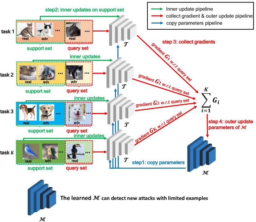
Figure 1. The procedure of MetaAdvDet training in one mini-batch (best viewed in color). The approach consists of a double-network framework: $\mathcal{M}$ and $\mathcal{T}$. $\mathcal{T}$ is the task-dedicated network which focuses on learning each task. It copies parameters from master network $\mathcal{M}$ at the beginning, and then trains on the support set. After a couple of iterations (inner update step), $\mathcal{T}$ converges and computes the gradient $G_{i}$ on the query set of task $i$. $\mathcal{M}$ accumulates the gradients $\sum_{i=1}^{K}G_{i}$ to update its parameters $\mathcal{M}_{\theta}$ which is prepared for the next mini-batch learning. The learned $\mathcal{M}$ can be used to detect new attacks with limited new samples. More details can be found in Sec.3.2 and Algorithm 1.

1. Introduction

The evolving adversarial attacks threaten the deep convolutional neural networks (DNNs) via adding human-imperceptible perturbation to clean images and thus lead to incorrect prediction. Various defense methods have been proposed for detecting attacks, which distinguish adversarial images and real images via capturing the features of DNNs under attacks (Ma et al., 2018; Bhagoji et al., 2017; Tian et al., 2018; Xu et al., 2018). However, new attack methods keep constantly evolving and yield new adversarial examples to bypass existing detector. For example, C&W attack (Carlini and Wagner, 2017) is proposed to circumvent all existing detection techniques at that time. Certain detection techniques have been proposed to detect new attacks (Sorin et al., 2002; Dathathri et al., 2018), these techniques are promising. However, most of them need tens of thousands of examples to train which are infeasible in practice. Because new attacks evolve much faster than the high-cost data collection, which results in a few-shot learning problem with evolving attacks. This issue makes the detection of adversarial examples still challenging.

Therefore, we study on how to tackle such few-shot learning problem, and propose a meta-learning based training approach with the learning-to-learn strategy. It focuses on learning to detect new attack from one or few instances of that attack. We name our approach as MetaAdvDet, refers to Meta-learning Adversarial Detection approach. To this end, the approach is equipped with a double-network framework for learning from tasks, which is defined as the small data collection with real examples and randomly chosen type of attacks. The purpose of introducing the tasks is to simulate new attack scenarios. To better learn from tasks, MetaAdvDet uses one network to focus on learning individual tasks, and the other network to learn the general detection strategy over multiple tasks. Fig. 1 illustrates the training procedure of one mini-batch, more details are described in Sec. 3.2. Each task is divided into support set and query set, which are used for learning either basic detection capability on old attacks, or minimizing the test error on new attacks. After training, the framework efficiently detects new attack with fine-tuning on limited examples. In contrast, the DNN based methods that use‘ the traditional training approach perform much worse in detecting new attacks than ours.

To comprehensively validate the detection techniques in terms of evolving attacks, we propose evaluations in following dimensions to validate the superiority of our approach in the few-shot problem.

Cross-adversary Dimension. To assess the capability of detecting new types of attacks in test set with few-shot samples..

Cross-domain Dimension. To assess the capability of detecting all attacks across different domains with few-shot samples.

Cross-architecture Dimension. To assess the capability of detecting the adversarial examples that are generated by attacking the classifier with new architecture.

White-box attack dimension. To assess the capability of detecting white-box attacks with few-shot samples.

To validate the effectiveness of our approach from above dimensions, we propose benchmarks with the few-shot-fashion protocol on three conventional datasets, i.e. CIFAR-10, MNIST and Fashion-MNIST datasets. The benchmarks include the generated adversarial examples by using various types of attacks, and it also defines the partition of train set and test set to simulate the scenario of testing the evolving attack’s detection.

In experiments, we compare our approach with end-to-end state-of-the-art methods using these benchmarks, and the results show that our approach surpasses the existing method by a large margin.

We summarize the main contributions below:

(1) To the best of our knowledge, we are the first to define the adversarial attack detection problem as a few-shot learning problem of detecting evolving new attacks.

(2) We propose a meta-learning based approach: MetaAdvDet, it is equipped with a double-network framework with the learning-to-learn strategy for detecting evolving attacks. Benefiting from the learning-to-learn strategy, our approach is able to achieve high performance in detecting new attacks.

(3) To comprehensively validate our approach in terms of evolving attacks, we construct benchmarks with the few-shot-fashion protocol on three datasets, i.e. CIFAR-10, MNIST and Fashion-MNIST. The benchmarks define the partition of train set and test set to simulate the scenario of testing the evolving attack. We believe the proposed benchmark is useful for the future research of defending evolving attacks.

2. Background

Many attempts have been made to detect or defense against adversarial attack. We first introduce the defense techniques, and then we introduce the meta-learning techniques that related to our work.

2.1. Defense Techniques

The adversary algorithm is used to generate the adversarial examples which makes the classifier to output incorrect prediction. Many defense techniques have been proposed to defend against adversarial attack, these techniques generally fall into two categories.

The first category attempts to build a robust model that classifies the adversarial example correctly, such as (Papernot et al., 2016c; Akhtar et al., 2018; Song et al., 2018; Liao et al., 2018). However, certain new attacks (Chen et al., 2017; Li et al., 2019) are deliberately implemented to grasp the weakness of these methods to circumvent the defense. For example, Athalye et al. (Athalye et al., 2018) identifies the obfuscated gradients, which is a kind of gradient masking, that leads to a false sense of security in defenses. Based on their findings, the new attacks are proposed to circumvent 7 of 9 defenses relying on obfuscated gradients.

Due to the difficulty, the second category of defense techniques turn to distinguish the adversarial examples from real ones, in order to improve security and detect malicious users. This category refers to adversarial attack detection. Unlike the first category, adversarial detection does not need to classify the adversarial image correctly, but only to identify them. Essentially, a detector is also a binary classifier which is trained on the real and adversarial examples. Based on this idea, certain detection techniques (Carrara et al., 2017; Sorin et al., 2002; Metzen et al., 2017) build a subnet classifier to capture the hidden layer’s features of the adversarial example. Other methods include (1) capturing the difference of DNN’s output between real and adversarial images when applying certain transformation to the input images (Tian et al., 2018; Xu et al., 2018; Dathathri et al., 2018; Bhagoji et al., 2017), (2) utilizing the intrinsic dimensionality of adversarial regions (Ma et al., 2018), (3) employing new loss function to encourage DNN to learn a more distinguishable representation (Pang et al., 2018; Wan et al., 2018), (4) using statistical test (Grosse et al., 2017), and (5) using the capsule network (Frosst et al., 2018).

However, the high-cost data collection cannot keep up with the evolution frequency of the attacks, which leads the training for detecting new attacks difficulty. For example, when a new attack first appears without publishing the source code, most of defenders have insufficient examples to train the detector. This situation makes the issue of detecting evolving attacks highly urgent. We categorize this issue as a new defense problem, which is a few-shot learning problem of detecting evolving attacks.

2.2. Meta-Learning

Few-shot learning problem (Vinyals et al., 2016; Snell et al., 2017) has been studied for a long time, which is defined as learning from few samples. The meta-learning techniques (Finn et al., 2017; Li et al., 2017; Erin Grant and Griffiths, 2018; Mishra et al., 2018; Jamal and Qi, 2019) are promising for addressing the few-shot learning problem, which usually trains a meta-learner on the distribution of few-shot tasks so that the it can generalize and perform well on the unseen task. Model-agnostic meta-learning (MAML) (Finn et al., 2017) is a typical meta-learning approach, which learns a internal representation that is widely suitable for many tasks. It learns a proper weight initialization on the support set and then updates itself to perform well on the query set. To update the weights more efficiently, Meta-SGD (Li et al., 2017) makes the meta-learner not only to learn the weight initialization but also update direction and learning rate. For better understanding in this field, we introduce the terminologies of meta-learning, as describe below.

Task: A meta-learning model (meta-learner) should be trained over a variety of tasks and optimized for the best performance on the task distribution, including potentially unseen tasks. The concept of “task” in this paper is totally different from the concept of “multi-task learning”, but only a manner of data partition that the meta-learner used to train.

Support&query set: Each task is split into two subsets, which are the support set for learning the basic classification on old tasks, and the query set for training in the train stage or testing in the test stage. It should be emphasized that the support set and query set from the same task have the same data distribution.

Way is the class in each task that the meta-learner wish to discriminate, whose number may be specified arbitrarily and do not need to equal the ground truth class number.

Shot is the number of samples in each way of the support set. For example, an $N$-way, $K$-shot classification task includes the support set with $K$ labeled examples for each of $N$ classes.

Based on the spirit of meta-learning, we propose the training method with a double-network framework and introduce the double-update scheme for achieving fast adaption capacity. Experiments show the superiority of our approach in detecting new attacks.

3. Approach

3.1. Overview

The evolving adversarial attacks are hard to distinguish due to the insufficient new adversarial examples for training the detector, results in the few-shot learning problem. One of the keys for solving this problem is to use the power of meta-learning techniques. Typical meta-learning methods (e.g. MAML (Finn et al., 2017)) are trained for learning the task distribution. Because the categories of data in each task are randomly chosen, the meta-leaner acquires fast adaption capability to unseen data type via learning these tasks. To model the attack detection technique in the meta-learning style framework, we collect various types of attacks to construct adversarial example dataset into the multiple tasks form (Fig. 2). Each task is a small data collection with a randomly chosen attack which represents one attacking scenario, so the large amount of tasks make the meta-learner experience various attacking scenarios, so that it can adapt to new attacks rapidly. Our approach is equipped with a double-network framework with learning-to-learn strategy, which focuses on learning how to learn new tasks faster by reusing previous experience, rather than considering new tasks in isolation. Specifically, one network of our framework focuses on learning from individual tasks (named task-dedicated network $\mathcal{T}$), the other network updates its parameters based on the gradient accumulated from the $\mathcal{T}$ (named master network $\mathcal{M}$), to learn a general strategy over all tasks (Fig. 1). This double-network framework leads to the double update scheme, corresponding to the two networks.

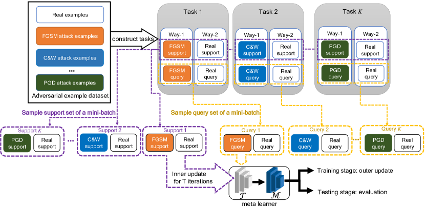
Figure 2. The details of constructing tasks for training and testing the meta-learner (including $\mathcal{T}$ and $\mathcal{M}$). Each task (support&query set) is sampled independently from the dataset, and each mini-batch consists of $K$ tasks. The training employs a double-update scheme: inner update and outer update. The inner update represents that $\mathcal{T}$ learns on support set, and the outer update represents $\mathcal{M}$ updates with the accumulated gradients of $\mathcal{T}$ on query set (as described in Fig. 1 and Sec. 3.2). $\mathcal{M}$ can be used to detect new attacks.

Fig. 2 shows the details of constructing tasks for training and testing the meta-learner, Fig. 1 demonstrates the procedure of training in one mini-batch, detailed steps are shown in Algorithm 1.

3.2. Learning MetaAdvDet

As we mentioned earlier, the learning-to-learn strategy is proposed to learn new attacks by reusing previous experience of detecting old attacks. Following the typical setting of meta-learning, all the training data are organized into tasks, each task is divided to two subsets, namely, the support set for learning basic capability of detecting old attacks, and the query set acts as the surrogate of new attacks for achieving rapid adaption in detecting new attacks of test set. To learn the tasks, the meta-learner includes a double-network framework, i.e. the master network $\mathcal{M}$, and a task-dedicated network $\mathcal{T}$ which is cloned from $\mathcal{M}$ to learn from individual tasks. $\mathcal{T}$ updates its parameters $\mathcal{T}_{\theta}$ based on each task’s support set, and then it calculates its gradient of the query set, which will be accumulated to update $\mathcal{M}$’s parameters $\mathcal{M}_{\theta}$ (Fig. 1). The same $\mathcal{M}_{\theta}$ will be copied and overwritten to the $\mathcal{T}_{\theta}$ before learning next task. The $\mathcal{M}$ and $\mathcal{T}$ output the classification probability to distinguish the real and adversarial example, corresponding to the two-way configuration. The two-way configuration stipulates that one of the ways should use real examples in all tasks. Two options are considered, i.e. the randomized-way setting, whose two-way labels are shuffled in each task; and the fixed-way setting, which uses label 1 for real example and label 0 for adversarial example in all tasks. We will compare the effect of above two options in Sec. 5.4.

Algorithm 1 shows the training procedure, Fig. 1 shows the detail of one mini-batch training procedure. $\mathcal{T}$ copies the all the parameters from $\mathcal{M}$ at the beginning of learning task $\mathbb{T}_{i}$, where the subscript $i$ denotes the task index. Then, the inner update step updates the parameters of $\mathcal{T}$ by using the support set of $\mathbb{T}_{i}$ for multiple iterations. Line 8 and line 9 demonstrate this step, which is the same with the supervised learning in the traditional DNN: we directly feed input images to $\mathcal{T}$ and uses the gradient descent to update its parameters based on the classification ground truth. Unlike existing methods that applying transformation on input images (Tian et al., 2018; Xu et al., 2018), we should note that the input image is not applied any transformation in this step of our approach. Finally, the meta-learner acquires rapid adaption capability by considering to minimize the test error on new data, this is the role that the outer update step upon the query set plays. More specifically, we calculate the cross entropy loss $\mathcal{L}$ on the query set of task $\mathbb{T}_{i}$ to obtain the gradient $G_{i}$ w.r.t. $\mathcal{T}_{\theta}$, which is accumulated from learning all tasks $\mathbb{T}_{1},\dotsc,\mathbb{T}_{K}$ and finally sent to $\mathcal{M}$. Because $\mathcal{M}$ and $\mathcal{T}$ use the same network structure and parameters, the accumulated gradient can be used to update parameters of $\mathcal{M}$, namely $\mathcal{M}_{\theta}$. Thus, $\sum_{i=1}^{K}G_{i}$ updates the $\mathcal{M}_{\theta}$ for learning the strategy over the multi-task distribution.

Algorithm 1 MetaAdvDet training procedure

master network $\mathcal{M}$ and its parameters $\mathcal{M}_{\theta}$, task-dedicated network $\mathcal{T}$ and its parameters $\mathcal{T}_{\theta}$, the feed-forward function $f_{\mathcal{T}_{\theta}}$ of $\mathcal{T}$, max iterations $N$, inner-update learning rate $\lambda_{1}$, outer-update learning rate $\lambda_{2}$, inner updates iteration $T$, the multi-task format dataset $\mathcal{D}$, cross entropy loss function $\mathcal{L}$.

the learned network $\mathcal{M}$

1:for $iter\leftarrow 1$ to $N$ do

2:     sample $K$ tasks $\mathbb{T}_{i,i\in\{1,\cdots,K\}}$ from $\mathcal{D}$

3:     for $i\leftarrow 1$ to $K$ do

4:         $S_{i}$ and $Q_{i}$ $\leftarrow$ support set and query set of $\mathbb{T}_{i}$

5:         $\mathcal{T}_{\theta}\leftarrow\mathcal{M}_{\theta}$$\triangleright$ copy parameters from $\mathcal{M}$ to $\mathcal{T}$

6:         $\mathcal{T}_{\theta^{\prime}}\leftarrow\mathcal{T}_{\theta}$$\triangleright$ $\mathcal{T}_{\theta}$ will be used in the outer update

7:         for $t\leftarrow 1$ to $T$ do

8:              Calculate $\nabla_{\mathcal{T}_{\theta^{\prime}}}\mathcal{L}(f_{\mathcal{T}_{\theta^{\prime}}})$ by using $S_{i}$

9:              $\mathcal{T}_{\theta^{\prime}}\leftarrow\mathcal{T}_{\theta^{\prime}}-\lambda_{1}\nabla_{\mathcal{T}_{\theta^{\prime}}}\mathcal{L}(f_{\mathcal{T}_{\theta^{\prime}}})$ $\triangleright$ inner update

10:         end for

11:         $G_{i}\leftarrow\nabla_{\mathcal{T}_{\theta}}\mathcal{L}(f_{\mathcal{T}_{\theta^{\prime}}})$ by using $Q_{i}$

12:     end for

13:     $\mathcal{M}_{\theta}\leftarrow\mathcal{M}_{\theta}-\lambda_{2}\sum_{i=1}^{K}G_{i}$ $\triangleright$ outer update

14:end for

15:return $\mathcal{M}$

Following popular few-shot-fashion testing procedure (Ravi and Larochelle, 2017), the evaluation restricts that the method needs to be evaluated on all test tasks. Algorithm 2 shows the testing procedure. The few-shot-fashion testing procedure should include a fine-tune step by using few-shot examples, as shown in line 6 of Algorithm 2. In experiments, we adopt a general binary classifier with DNN as the baseline for comparison. DNN uses a single network for training, whereas MetaAdvDet uses a double-network framework to obtain the learning-to-learn strategy. The experiment proves the superiority of our approach in detecting new attacks (Sec. 5.5).

Algorithm 2 MetaAdvDet testing procedure

master network $\mathcal{M}$ and its learned parameters $\mathcal{M}_{\theta}$, task-dedicated network $\mathcal{T}$ and its parameters $\mathcal{T}_{\theta}$, the feed-forward function $f_{\mathcal{T}_{\theta}}$ of $\mathcal{T}$, fine-tune iterations $T$, learning rate $\lambda$, test tasks $\mathbb{T}_{i,i\in\{i,\cdots,N\}}$ which is obtained by reorganizing the test set, cross entropy loss $\mathcal{L}$, ground truth $Y_{i,i\in\{i,\cdots,N\}}$ of the query set.

the average F1 score over all tasks

1:for $\mathbb{T}_{i}\leftarrow\mathbb{T}_{1}$ to $\mathbb{T}_{N}$ do $\triangleright$ iterate over all test tasks

2:     $S_{i}$ and $Q_{i}$ $\leftarrow$ support set and the query set of $\mathbb{T}_{i}$

3:     $\mathcal{T}_{\theta}\leftarrow\mathcal{M}_{\theta}$$\triangleright$ copy parameters to ensure each task is tested independently

4:     for $t\leftarrow 1$ to $T$ do

5:         Calculate $\nabla_{\mathcal{T}_{\theta}}\mathcal{L}(f_{\mathcal{T}_{\theta}})$ by using $S_{i}$

6:         $\mathcal{T}_{\theta}\leftarrow\mathcal{T}_{\theta}-\lambda\nabla_{\mathcal{T}_{\theta}}\mathcal{L}(f_{\mathcal{T}_{\theta}})$ $\triangleright$ fine-tune step

7:     end for

8:     $\hat{Y}_{i}\leftarrow f_{\mathcal{T}_{\theta}}(Q_{i})$ $\triangleright$ get prediction of query set of task $i$

9:     $\text{score}_{i}\leftarrow\text{F1}(\hat{Y}_{i},Y_{i})$

10:end for

11:$\text{F1 score}\leftarrow\frac{1}{N}\sum_{i=1}^{N}score_{i}$

12:return F1 score

The F1 score of the query set is adopted as the metric for evaluating the performance of detection techniques (Sec. 5.2). Note that the F1 score is calculated upon individual tasks, the final F1 score is obtained via averaging F1 scores of all tasks, which follows the few-shot-fashion testing procedure of MiniImagenet (Ravi and Larochelle, 2017), steps are shown in line 11 of Algorithm 2. All the compared methods should use this metric and include the fine-tune step for fair comparison.

4. Proposed Benchmark

4.1. Adversarial Example Datasets Construction

In order to validate the effectiveness of our approach, we construct the adversarial example datasets based on the conventional datasets. The built datasets use fifteen adversaries to yield examples whose data sources come from CIFAR-10 (Krizhevsky, 2009), MNIST (LeCun and Cortes, 2010) and Fashion-MNIST (Xiao et al., 2017) datasets, named AdvCIFAR, AdvMNIST and AdvFashionMNIST respectively. To train the detectors for distinguishing real examples and adversarial examples, each dataset includes an additional real example’s category whose data are directly transfered from original dataset (i.e. CIFAR-10 etc.). All fifteen types of adversarial examples are generated by utilizing CleverHans library (Papernot et al., 2018), which attacks the classifiers with three architectures for each adversary, namely 4 conv-layers network (conv-4), ResNet-10 (He et al., 2016) and ResNet-18 (He et al., 2016). Note that MI-FGSM, BIM and PGD attacks adopt the $\ell_{\infty}$ norm version, C&W and Deepfool attacks adopt the $\ell_{2}$ norm version. Such adoptions are based on the attack successful rate. In addition, the adversarial examples of L-BFGS attack (Szegedy et al., 2014) is used as the validation set. The BPDA attack (Athalye et al., 2018) that utilizes the obfuscate gradients of defense is not used, because our approach does not reply on obfuscate gradients. The statistical data for the adversarial example datasets are shown in Tab. 1.

Table 1. Our adversarial example datasets contain the examples generated by attacking different architectures, including a 4 conv-layers network (conv-4), ResNet-10 and ResNet-18.This table lists the amount of adversarial examples which are generated by successfully attacking the conv-4 network.

adversary	AdvCIFAR		AdvMNIST		AdvFashionMNIST
	train	test	train	test	train	test
FGSM (Goodfellow et al., [n. d.])	$46,851$	$9260$	$23,646$	$3853$	$48,368$	$7999$
MI-FGSM (Dong et al., 2018)	$46,742$	$9205$	$58,445$	$9701$	$56,744$	$9362$
BIM (Kurakin et al., 2017)	$46,076$	$9118$	$58,522$	$9715$	$56,587$	$9341$
PGD (Madry et al., 2018)	$47,911$	$9504$	$58,439$	$9693$	$57,060$	$9428$
C&W (Carlini and Wagner, 2017)	$47,810$	$9509$	$58,121$	$9651$	$57,072$	$9435$
jsma (Papernot et al., 2016b)	$49,141$	$9807$	$26,377$	$4305$	$39,804$	$6770$
EAD (Chen et al., 2018)	$45,146$	$8908$	$59,458$	$9885$	$56,157$	$9283$
SPSA (Uesato et al., 2018)	$42,183$	$8436$	$1260$	$245$	$12,604$	$2225$
Spatial Transformation (Xiao et al., 2018)	$47,075$	$9320$	$58,820$	$9770$	$59,520$	$9917$
VAT (Miyato et al., 2016)	$28,758$	$5788$	$11,392$	$1869$	$24,774$	$4159$
semantic (Hosseini et al., 2017)	$31,704$	$6415$	$52,398$	$8723$	$47,401$	$7918$
MaxConfidence (Goodfellow et al., 2019)	$48,293$	$9565$	$57,676$	$9604$	$57,309$	$9469$
Deepfool (Moosavi-Dezfooli et al., 2016)	$44,740$	$8879$	$59,461$	$9886$	$56,171$	$9294$
NewtonFool (Jang et al., 2017)	$45,240$	$8916$	$59,473$	$9884$	$56,249$	$9294$
L-BFGS (Szegedy et al., 2014)(validation set)	$9683$		$9583$		$9598$

4.2. Cross-Adversary Benchmark

To validate the effectiveness of detection techniques in detecting new attacks, we configure the train set and test set contain no common type of adversarial examples to simulate this situation. To this end, the attacks are grouped based on their categories, and we propose the cross-adversary benchmark which assigns the different adversary groups to the train set and test set.

Table 2. The definition of adversary groups in the cross-adversary benchmark.

Train Adversary Group	Test Adversary Group	Validation	Train&Test
FGSM, MI-FGSM, BIM, PGD, C&W, jsma, SPSA, VAT, MaxConfidence	EAD, semantic, Deepfool, Spatial Transformation, Newtonfool	L-BFGS	same domain

Tab. 2 shows the adversary groups of cross-adversary benchmark. The grouping principles of this benchmark are: (1) each adversary should be assigned to one group only. (2) The similar adversaries should be assigned into the same group. For example, the MI-FGSM adversary is a modification of FGSM, and thus they are similar and we make them into one group. Based on this benchmark, the train set and test set should not include attacks of the same group simultaneously. Note that in this benchmark, the adversaries of train group extract the train set of the adversarial example dataset (e.g. train set of FGSM in Tab. 1) to train the detectors. Similarly, the detectors are evaluated on the test set of the test group’s adversaries.

4.3. Cross-Domain Benchmark

Table 3. The cross-domain benchmark consists of 2 protocols on the AdvMNIST and AdvFashionMNIST.

Protocol	Train Domain	Test Domain	Attack Types	Test Shots
#1	AdvMNIST	AdvFashionMNIST	all attacks	1-shot, 5-shot
#2	AdvFashionMNIST	AdvMNIST	all attacks	1-shot, 5-shot

The concept of a domain indicates an adversarial dataset, e.g. AdvMNIST. Since different domains have different data distributions, which leads the cross-domain benchmark to a more challenging benchmark. To evaluate the capability of detecting the adversarial examples generated from new domain, the detectors are trained one domain (Train Domain), and tested on the other domain (Test Domain). In this benchmark, we focus on the transferability between two datasets, namely AdvMNIST and AdvFashionMNIST, as listed in Tab. 3. Note that in this benchmark, all types of the attacks are used to train the detector.

4.4. Cross-Architecture Benchmark

Table 4. The cross-architecture benchmark consists of 4 protocols, this benchmark indicates the examples of train set and test set are generated by attacking different networks.

Protocol	Train Arch	Test Arch	Attack Types	Test Shots	Train&Test
#1	ResNet-10	ResNet-18	all attacks	1-shot, 5-shot	same domain
#2	ResNet-18	ResNet-10	all attacks	1-shot, 5-shot	same domain
#3	conv-4	ResNet-10	all attacks	1-shot, 5-shot	same domain
#4	ResNet-10	conv-4	all attacks	1-shot, 5-shot	same domain

Existing studies show that the adversarial examples generated by attacking one architecture can fool another architecture (Papernot et al., 2016a; Liu et al., 2017). To validate the detection capability in this situation, this benchmark stipulates that the train set and test set should include the adversarial examples come from attacking different architectures. For example, the detector is trained on the adversarial examples generated by attacking a classifier with the conv-4 network (Train Arch), but tested on the ones of ResNet-10 (Test Arch). Tab. 4 shows the detail of this benchmark, all types of attacks are used to train the detectors. Three architectures are used, namely conv-4, ResNet-10 and ResNet-18. Note that the concept of architecture in this benchmark is only related to the classifier’s backbone during adversarial examples generation, but not related to the detector model.

4.5. White-box Attack Benchmark

The white-box attack means the adversary has the information of both the image classifier and is aware of the detector. It has full knowledge of the detector. In other words, the adversary needs to fool both the classifier and detector simultaneously, making it more challenge to defend. We use the targeted iterative FGSM (I-FGSM) (Kurakin et al., 2017) and C&W (Carlini and Wagner, 2017) attacks to simulate white-box attacks with the method presented in Carlini and Wagner (Carlini and Wagner, 2017). The basic idea is to construct a combined model which combines the original classifier model and the detector. The original classifier has $N$ output labels, then the new model outputs $N+1$ labels with the last label indicates whether the input is an adversarial example. More specifically, let’s denote the new model as $B$ which combines the classifier $C$ and the detector $D$. $B$’s output logits is denoted as $Z_{B}$, $C$’s output is denoted as $Z_{C}$ and $D$’s output as $Z_{D}$. The $Z_{B}$ is constructed using the following formula:

(1) $$Z_{B}(x)_{i}=\begin{cases}Z_{C}(x)_{i}&\text{if }i\leq N\\ Z_{D}(x)\times 2\times\text{max}Z_{C}(x)&\text{if }i=N+1\end{cases}$$

It is easy to see that when an input is detected as an adversarial example by $D$, then $Z_{D}$ would be larger than 0.5 and it leads $Z_{B}(x)_{N+1}$ to be larger than $Z_{B}(x)_{i}$ for $1\leq i\leq N$. If an input is detected as a real example, $B$ classifies it the same label as $C$ does. In this way, the new model $B$ combines $C$ and $D$.

Now, we can use the targeted iterative FGSM (I-FGSM) or C&W adversary to attack this new model $B$ to generate the white-box adversarial example. The target label is set to make $C$ classify this example incorrectly but make the example bypass the detector $D$. In MetaAdvDet, $D$ represents for the learned master network $\mathcal{M}$ which would be attacked. Although the white-box attack leads $\mathcal{M}$ to misclassify, MetaAdvDet can benefit from the learning-to-learn strategy for recovering to the correct prediction with limited white-box examples provided, as steps shown in Algorithm 2.

5. Experiment

5.1. Experiment Setting

Table 5. The modules of one block in the conv-3 backbone of MetaAdvDet and other compared methods. The conv-3 backbone consists of 3 such blocks in total, and the last block connects to a fully-connected layer to output a vector with two probabilities.

index	module	parameter configuration
1	conv-layer	3$\times$3 kernel, channel = 64, pad = 0
2	batch normalization	momentum = 1
3	ReLU	-
4	max pooling	2$\times$2 pooling, stride = 2

Table 6. The default parameters configuration which is used in the ablation study in Sec. 5.4, and also used in other comparative experiments of Sec. 5.5, Sec. 5.6, Sec. 5.7 and Sec. 5.8.

name	default value	description
shots	1	number of examples in a way, MetaAdvDet should set the same shots in both training and testing.
ways	2	alias of class number, data of the same way come from using the same adversary to attack the same category’s images.
train query set size	70	number of examples of a query set in training.
test query set size	30	number of examples of a query set in testing.
task number $K$	30	number of tasks in each mini-batch.
inner update times	12	iteration times of inner update during training
fine-tune times	20	iteration times of fine-tune during testing.
total tasks	20000	total tasks in the constructed tasks.
inner learning rate	0.001	learning rate of inner update.
outer learning rate	0.0001	learning rate of outer update.
dataset	AdvCIFAR	the dataset for ablation study
backbone	conv-3	the backbone of MetaAdvDet & compared methods
benchmark	cross-adversary	the benchmark for ablation study

In the construction of tasks, we set the task number to be $20,000$ in total, which covers all the samples of the original datasets. During the learning process, 30 tasks are randomly chosen from these tasks to form each mini-batch. In each task, the two-way setting is applied which makes MetaAdvDet to be a binary classifier for distinguishing the adversarial examples from real examples, as shown in Fig. 2. The inner-update learning rate $\lambda_{1}$ is set to $0.001$ empirically. Because of the summation of gradients in Algorithm 1, the outer-update learning rate $\lambda_{2}$ is set to $0.0001$ which is 10 times smaller than $\lambda_{1}$. The training epoch is set to 4, because after 4 epochs, we observe that the F1 score on the validation set is stable. The query set size used for outer-update is set to 70 for two ways, that is 35 samples in each way. The fine-tune iteration times is set to 20 which reaches the stable performance (Fig. 4). All parameters configuration is shown in Tab. 6 which is set empirically based on validation set.

5.2. Evaluation Metric

Our metric restricts that all compared methods need to be evaluated on 1000 testing tasks to cover all test samples. To quantify the detection performance of all detection methods, we adopt the F1 score which follows Liang et al.(Liang et al., 2018) and Sabokrou et al.(Sabokrou et al., 2018). It is defined as the harmonic mean between precision and recall:

(2) $$\text{recall}=\frac{TP}{TP+FN},\text{precision}=\frac{TP}{TP+FP}$$

$$\text{F1}=2\times\frac{\text{precision}\times\text{recall}}{\text{precision}+\text{recall}}$$

We use label 1 to represent the real example and 0 to represent the adversarial example, so TP is the number of correctly detected real examples, FN is the number of real examples that are incorrectly detected as adversarial examples, and FP is the number of adversarial images that are detected as real examples. Note that the final F1 score is obtained via averaging F1 scores of all tasks (Algorithm 2).

5.3. Compared Methods

The selection of compared state-of-the-art methods are based on the consideration of two principles: (1) In order to comply with the few-shot-fashion benchmarks, the compared method must be an end-to-end learning approach to be fine-tuned in test stage. (2) The compared methods are able to detect new attacks, in order to evaluate and compare the detection technique in terms of evolving adversarial attacks. Based on above principles, MetaAdvDet is compared with a image rotation transformation based detector, named TransformDet (Tian et al., 2018); and a detection technique based on a secret fingerprint, named NeuralFP (Dathathri et al., 2018). The NeuralFP is trained for 100 epochs on each dataset, and TransformDet is trained for 10 epochs on each dataset. In the fine-tune step, because NeuralFP is trained on real examples, we extract the real examples from support set to fine-tune. In addition, NeuralFP obtains the F1 score via determining the best threshold for each task. We configure these methods following their original settings (Tian et al., 2018; Dathathri et al., 2018) (Tab. 7).

Table 7. The configuration of train, validation and test set of all compared methods on the proposed benchmarks.

Method	Train Set	Test Set	Validation Set
DNN	train set of adversarial example datasets (e.g. AdvCIFAR etc.)	constructed tasks of test set in adversarial example datasets, each task contains the support set and the query set. The performance is evaluated on the query set.	constructed tasks of validation set in adversarial example datasets, each task contains the support set and the query set. The performance is evaluated on the query set.
DNN (balanced)	train set of adversarial example datasets which is down-sampling to keep class balanced
NeuralFP (Dathathri et al., 2018)	real examples of train set in the original dataset (e.g. CIFAR-10 etc.)
TransformDet (Tian et al., 2018)	train set of adversarial example datasets, down-sampling if necessary.
MetaAdvDet	constructed tasks of train set in adversarial example datasets

We adopt a binary neural network classifier as the baseline, denotes as DNN. DNN is trained on all data of adversarial example dataset and its backbone is the same with MetaAdvDet, which is a 3 conv-layers network (Tab. 5). Because the adversarial example datasets are the highly class imbalance datasets which contain much more adversarial examples than real ones, we train the other DNN by using the balanced data between adversarial and real samples by down-sampling, which is denoted as DNN (balanced). The dataset configurations of different methods are listed in Tab. 7.

5.4. Ablation Study

To inspect the effect of each key parameter respectively, we conduct the control experiments on AdvCIFAR by adjusting one parameter while keeping other parameters fixed as listed Tab. 6. Fig. 3 and Fig. 4 are the results of the cross-adversary benchmark.

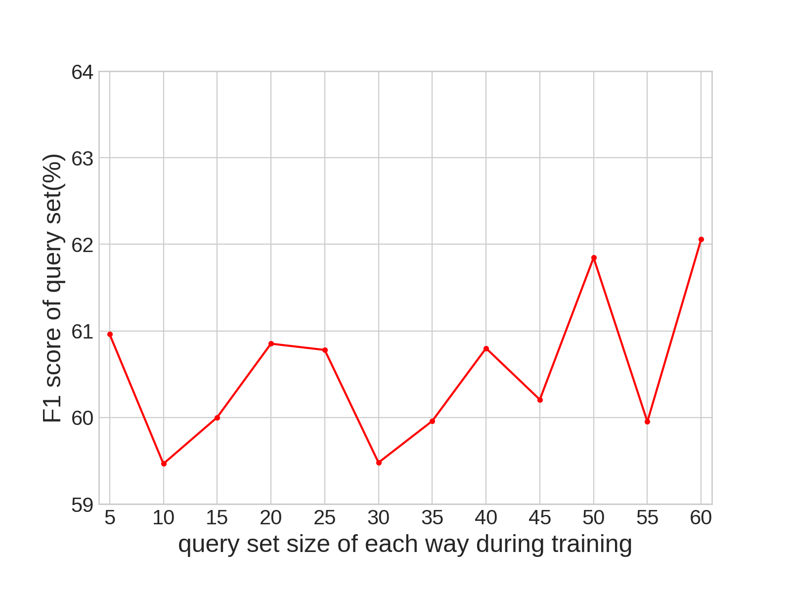
(a) train query set size study

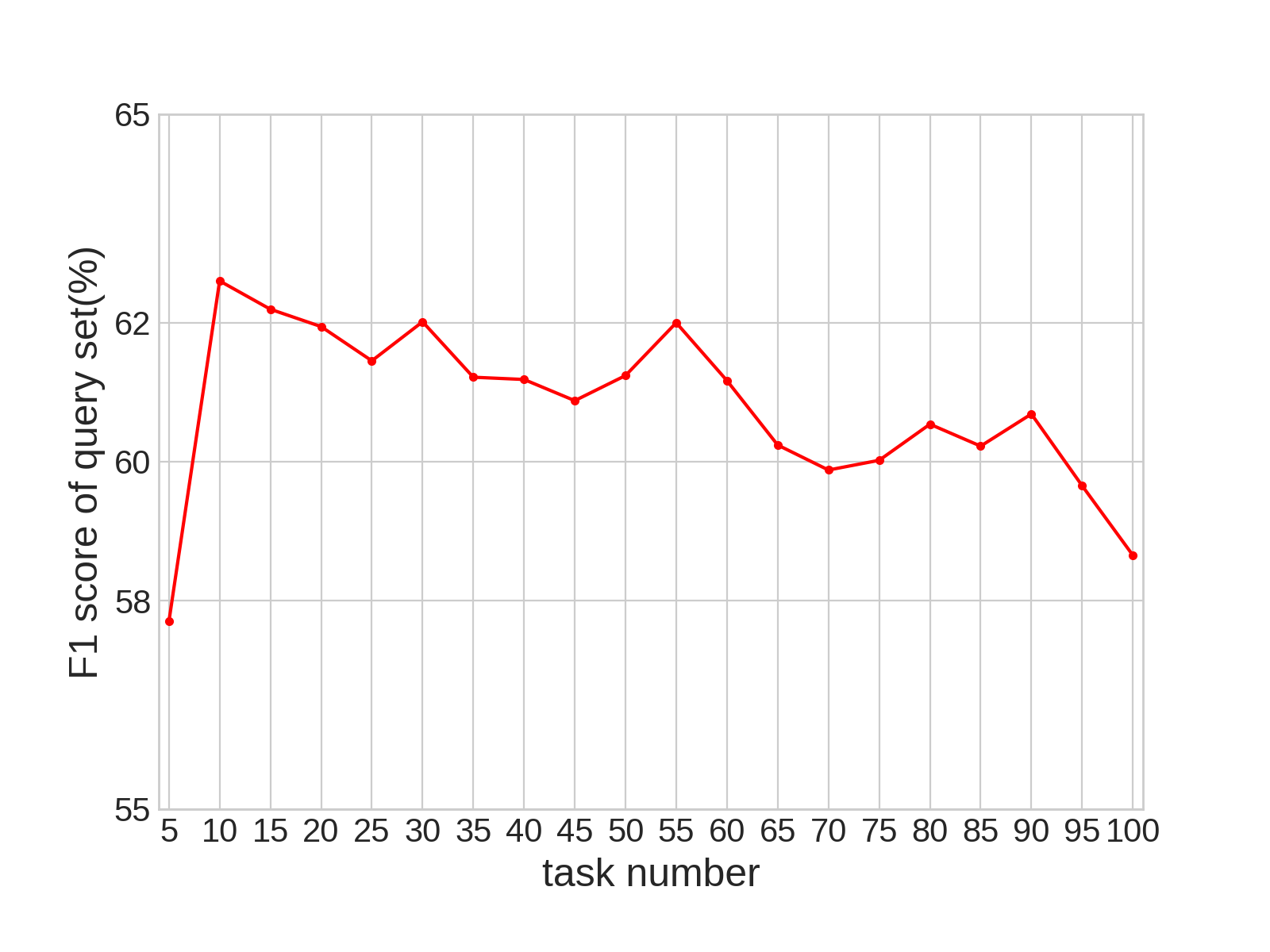
(b) task number $K$ study

Figure 3. Ablation study results of train query set size and task number of a training mini-batch.

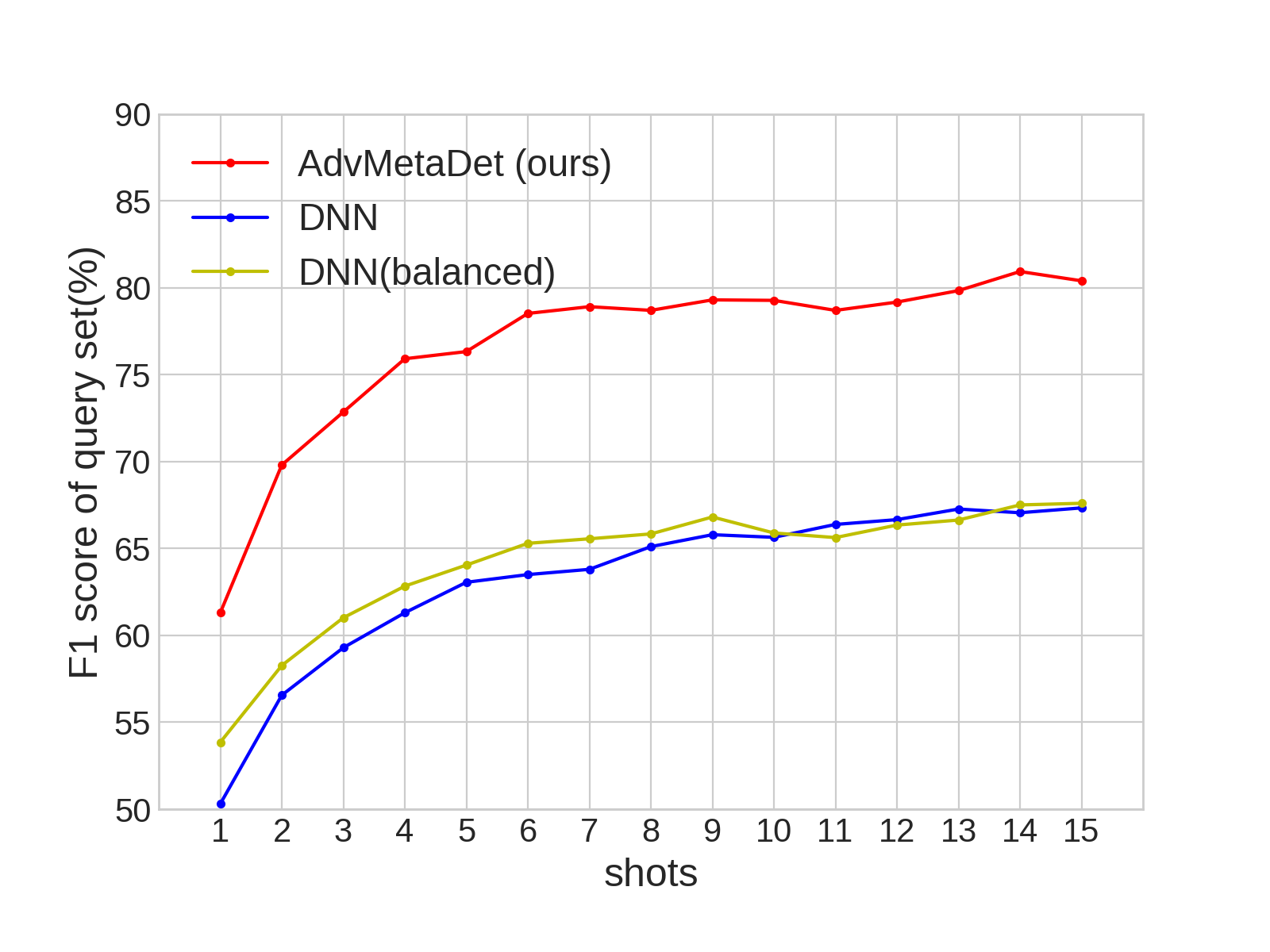
(a) shots study

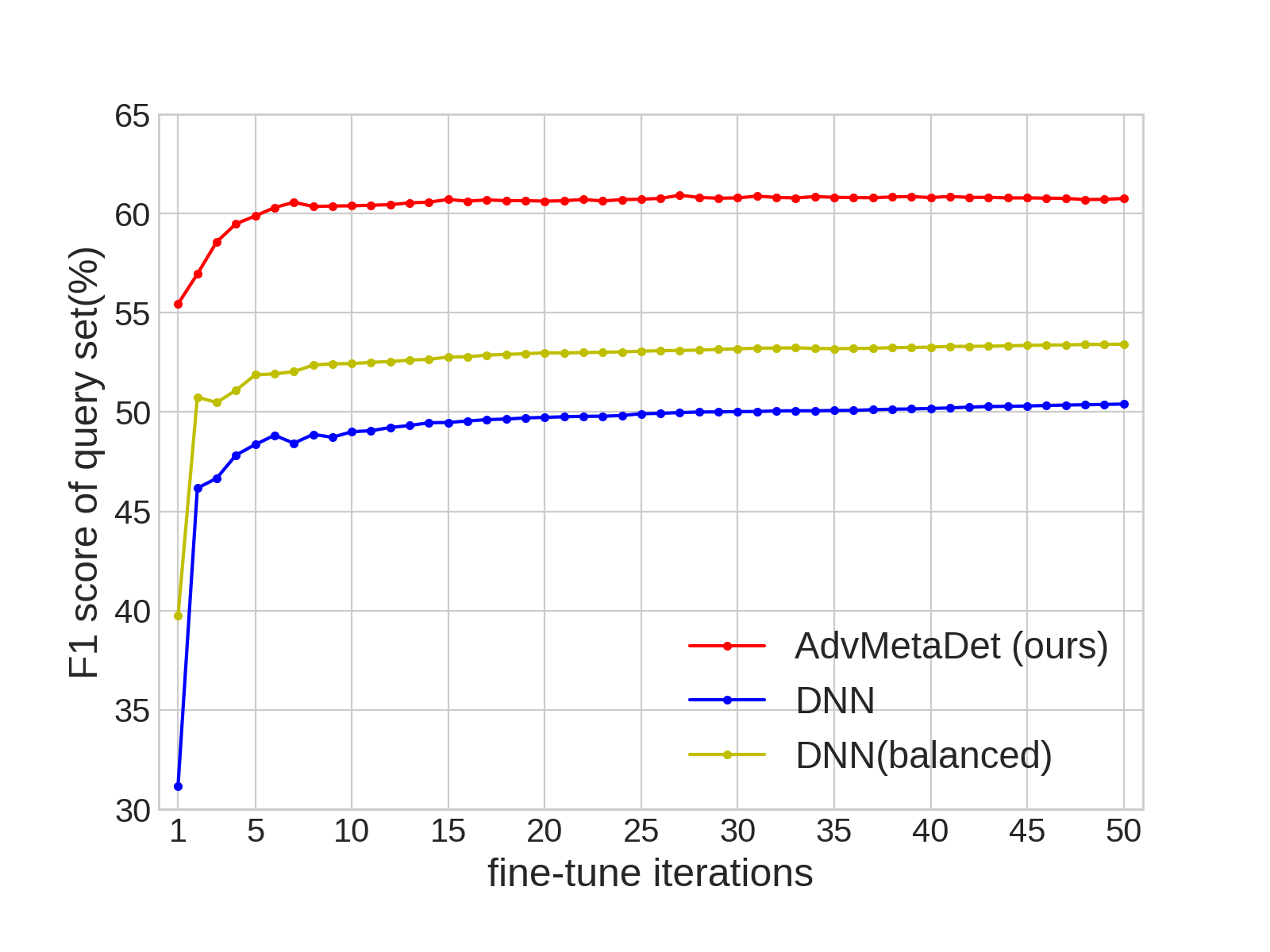
(b) fine-tune iterations study

Figure 4. Ablation study results of shots and fine-tune iterations. MetaAdvDet outperforms the baseline DNN and DNN (balanced) by a large margin.

From Fig. 4, following conclusions can be drawn:

1) MetaAdvDet outperforms DNN with only a few fine-tuning iterations, e.g. MetaAdvDet even surpasses the results of all fine-tune iterations of DNN by only using a single iteration (Fig. 4).

2) The balanced training data of DNN (balanced) helps to improve performance over DNN with the few-shot fine-tunings (Fig. 4).

Table 8. F1 score of randomized-way and fixed-way settings in AdvCIFAR. The randomized-way indicates that the labels of two ways are shuffled in each task. The fixed-way uses label 1 as real example and label 0 as adversarial example.

shots	fixed-way	randomized-way
1	0.686	0.616
5	0.787	0.772

Tab. 8 illustrates the F1 score results of a randomized-way and fixed-way assignment settings in AdvCIFAR dataset. It shows that the result of fixed-way setting outperforms that of randomized-way setting. In following experiments, we use the fixed-way setting.

5.5. Cross-Adversary Benchmark Result

To compare the performance of our approach and other state-of-the-art methods under the cross-adversary benchmark. In this section, we collect the results of TransformDet (Tian et al., 2018), NeuralFP (Dathathri et al., 2018), baseline DNN and DNN (balanced). Tab. 9 shows that MetaAdvDet outperforms the baseline and other methods in nearly all datasets. Thus, we can conclude MetaAdvDet is able to achieve high performance in detecting new attack with limited examples of that attack.

Our approach is particularly effective in detecting the attacks that exhibit quite different appearance from the training attacks. Typical representative attacks are Spatial Transformation, etc., the results of three representative attacks are shown in Tab. 10.

Table 9. F1 score of the cross-adversary benchmark, this table shows the results in using the adversarial examples generated by attacking the classifier with conv-4 architecture.

Dataset	Method	F1 score
		1-shot	5-shot
AdvCIFAR	DNN	0.495	0.639
	DNN (balanced)	0.536	0.643
	NeuralFP (Dathathri et al., 2018)	0.698	0.700
	TransformDet (Tian et al., 2018)	0.662	0.697
	MetaAdvDet (ours)	0.685	0.791
AdvMNIST	DNN	0.812	0.852
	DNN (balanced)	0.797	0.808
	NeuralFP (Dathathri et al., 2018)	0.780	0.906
	TransformDet (Tian et al., 2018)	0.840	0.904
	MetaAdvDet (ours)	0.987	0.993
AdvFashionMNIST	DNN	0.782	0.885
	DNN (balanced)	0.744	0.850
	NeuralFP (Dathathri et al., 2018)	0.798	0.817
	TransformDet (Tian et al., 2018)	0.712	0.879
	MetaAdvDet (ours)	0.848	0.944

Table 10. F1 score of representative adversaries on the AdvCIFAR dataset, cross-adversary benchmark.

Dataset	Adversary	Method	F1 score
			1-shot	5-shot
AdvCIFAR	Spatial Transformation (Xiao et al., 2018)	DNN	0.498	0.599
		DNN (balanced)	0.529	0.589
		NeuralFP (Dathathri et al., 2018)	0.708	0.696
		TransformDet (Tian et al., 2018)	0.633	0.660
		MetaAdvDet (ours)	0.811	0.920
	semantic (Hosseini et al., 2017)	DNN	0.488	0.644
		DNN (balanced)	0.529	0.657
		NeuralFP (Dathathri et al., 2018)	0.698	0.700
		TransformDet (Tian et al., 2018)	0.662	0.688
		MetaAdvDet (ours)	0.763	0.855
	NewtonFool (Jang et al., 2017)	DNN	0.511	0.664
		DNN (balanced)	0.542	0.670
		NeuralFP (Dathathri et al., 2018)	0.696	0.696
		TransformDet (Tian et al., 2018)	0.658	0.716
		MetaAdvDet (ours)	0.647	0.735

5.6. Cross-Domain Benchmark Result

Table 11. F1 score of the cross-domain benchmark, this table shows the results which are evaluated on the adversarial examples generated by attacking the conv-4 network. All the types of attacks are used to train the detectors.

Train Domain	Test Domain	Method	F1 score
			1-shot	5-shot
AdvMNIST	AdvFashionMNIST	DNN (balanced)	0.698	0.813
		NeuralFP (Dathathri et al., 2018)	0.748	0.811
		TransformDet (Tian et al., 2018)	0.664	0.808
		MetaAdvDet (ours)	0.799	0.870
AdvFashionMNIST	AdvMNIST	DNN (balanced)	0.950	0.977
		NeuralFP (Dathathri et al., 2018)	0.775	0.836
		TransformDet (Tian et al., 2018)	0.934	0.940
		MetaAdvDet (ours)	0.956	0.981

In the cross-domain benchmark, the models are trained in one domain, and tested in the other domain’s test set (Sec. 4.3). We use DNN (balanced) instead of DNN in this benchmark because the all types of attacks are used to train which results in the highly imbalanced data classification issue if using DNN. Tab. 11 shows the result, which demonstrates that MetaAdvDet has an advantage in hard test set. For example, when training on AdvMNIST and testing on AdvFashionMNIST, MetaAdvDet outperforms DNN (balanced) by a large margin (10.1% improvement in 1-shot).

Table 12. F1 score of cross-architecture benchmark.

Dataset	Train Arch	Test Arch	Method	F1 score
				1-shot	5-shot
AdvCIFAR	ResNet-10	ResNet-18	NeuralFP (Dathathri et al., 2018)	0.713	0.709
			TransformDet (Tian et al., 2018)	0.758	0.880
			DNN (balanced)	0.702	0.768
			MetaAdvDet (ours)	0.832	0.902
	ResNet-18	ResNet-10	NeuralFP (Dathathri et al., 2018)	0.712	0.703
			TransformDet (Tian et al., 2018)	0.788	0.874
			DNN (balanced)	0.711	0.752
			MetaAdvDet (ours)	0.840	0.889
	conv-4	ResNet-10	NeuralFP (Dathathri et al., 2018)	0.712	0.703
			TransformDet (Tian et al., 2018)	0.763	0.868
			DNN (balanced)	0.723	0.779
			MetaAdvDet (ours)	0.835	0.885
	ResNet-10	conv-4	NeuralFP (Dathathri et al., 2018)	0.709	0.702
			TransformDet (Tian et al., 2018)	0.766	0.885
			DNN (balanced)	0.739	0.790
			MetaAdvDet (ours)	0.854	0.918
AdvMNIST	ResNet-10	ResNet-18	NeuralFP (Dathathri et al., 2018)	0.906	0.882
			TransformDet (Tian et al., 2018)	0.973	0.988
			DNN (balanced)	0.943	0.972
			MetaAdvDet (ours)	0.984	0.993
	ResNet-18	ResNet-10	NeuralFP (Dathathri et al., 2018)	0.894	0.738
			TransformDet (Tian et al., 2018)	0.967	0.990
			DNN (balanced)	0.912	0.953
			MetaAdvDet (ours)	0.981	0.991
	conv-4	ResNet-10	NeuralFP (Dathathri et al., 2018)	0.894	0.738
			TransformDet (Tian et al., 2018)	0.972	0.985
			DNN (balanced)	0.897	0.959
			MetaAdvDet (ours)	0.963	0.983
	ResNet-10	conv-4	NeuralFP (Dathathri et al., 2018)	0.917	0.961
			TransformDet (Tian et al., 2018)	0.984	0.992
			DNN (balanced)	0.958	0.978
			MetaAdvDet (ours)	0.990	0.996
AdvFashionMNIST	ResNet-10	ResNet-18	NeuralFP (Dathathri et al., 2018)	0.813	0.856
			TransformDet (Tian et al., 2018)	0.936	0.974
			DNN (balanced)	0.848	0.932
			MetaAdvDet (ours)	0.960	0.979
	ResNet-18	ResNet-10	NeuralFP (Dathathri et al., 2018)	0.820	0.838
			TransformDet (Tian et al., 2018)	0.935	0.972
			DNN (balanced)	0.829	0.918
			MetaAdvDet (ours)	0.957	0.976
	conv-4	ResNet-10	NeuralFP (Dathathri et al., 2018)	0.820	0.838
			TransformDet (Tian et al., 2018)	0.946	0.970
			DNN (balanced)	0.920	0.968
			MetaAdvDet (ours)	0.946	0.975
	ResNet-10	conv-4	NeuralFP (Dathathri et al., 2018)	0.817	0.911
			TransformDet (Tian et al., 2018)	0.945	0.979
			DNN (balanced)	0.886	0.945
			MetaAdvDet (ours)	0.967	0.982

5.7. Cross-Architecture Benchmark Result

Tab. 12 shows the results of cross-architecture benchmark. Because NeuralFP is trained on the real samples, thus the same NeuralFP model is tested on the examples of different test architectures (Test Arch). Tab. 12 shows that MetaAdvDet outperforms other methods under different train and test architecture combinations, proving the superiority of MetaAdvDet in the cross-architecture benchmark.

5.8. White-box Attack Benchmark Result

In Tab. 13, we present the detection performance of the white-box benchmark. The NeuralFP (Dathathri et al., 2018) result is omitted because it detects the attack by setting threshold rather than conducting classification, which cannot be used in the method of Sec. 4.5. Tab. 13 shows that: (1) MetaAdvDet can effectively detect white-box attack even with only one white-box example provided. (2) White-box attack targets on the master network of the meta-learner in MetaAdvDet, whereas it targets on the detector itself in other methods.

Table 13. F1 score of white-box attack benchmark.

Dataset	Method	I-FGSM Attack		C&W Attack
		1-shot	5-shot	1-shot	5-shot
CIFAR-10	DNN (balanced)	0.466	0.537	0.459	0.527
	TransformDet (Tian et al., 2018)	0.593	0.728	0.443	0.502
	MetaAdvDet (ours)	0.553	0.633	0.548	0.607
MNIST	DNN (balanced)	0.857	0.956	0.814	0.913
	TransformDet (Tian et al., 2018)	0.864	0.952	0.775	0.893
	MetaAdvDet (ours)	0.968	0.994	0.920	0.990
FashionMNIST	DNN (balanced)	0.745	0.890	0.726	0.853
	TransformDet (Tian et al., 2018)	0.837	0.920	0.747	0.853
	MetaAdvDet (ours)	0.849	0.963	0.882	0.967

5.9. Inference Time

Table 14. The inference time(ms) of all methods.

Method	DNN	NeuralFP (Dathathri et al., 2018)	TransformDet (Tian et al., 2018)	MetaAdvDet (ours)
Inference time (ms)	$1.53\pm 0.01$	$2185.12\pm 18.10$	$69.17\pm 2.97$	$4.07\pm 4.40$

We further evaluate the inference time (excluding fine-tune steps) of all the methods measured in millisecond on one NVIDIA Geforce GTX 1080Ti GPU in Tab. 14. It shows that MetaAdvDet obtains the comparable inference time to DNN, due to that both methods use the same network architecture and the same feed-forward procedure for inference. In contrast, TransformDet applies multiple transformations on the input image which increases the inference time. NeuralFP tests multiple thresholds to determine the best threshold for detection, which significantly increases the inference time.

6. Conclusion

In this paper, we present a meta-learning based adversarial attack detection approach for detecting evolving adversary attacks with limited examples. To this end, the approach is equipped with a double-network framework which includes a task-dedicated network and a master network to learn from either individual tasks or the task distribution. In this way, the rapid adaption capability of detecting new attacks is achieved. Experimental results conclude that: (1) Tab. 9, Tab. 11 and Tab. 12 show that NeuralFP gets lower F1 scores than ours under different benchmarks. It manifests that NeuralFP which is trained on real examples cannot detect evolving attacks effectively. (2) We get the lowest results in AdvCIFAR dataset (Tab. 9, Tab. 12 and Tab. 13), which manifests the adversarial examples generated in CIFAR-10 are more difficult to detect. (3) MetaAdvDet performs well in the benchmarks of cross-adversary (Tab. 9), cross-domain (Tab. 11), cross-architecture (Tab. 12) and white-box attack (Tab. 13), proving that MetaAdvDet is a suitable method for detecting evolving attacks with limited examples.

References

- (1)
- Akhtar et al. (2018) Naveed Akhtar, Jian Liu, and Ajmal Mian. 2018. Defense against universal adversarial perturbations. In Proceedings of the IEEE Conference on Computer Vision and Pattern Recognition. 3389–3398.
- Athalye et al. (2018) Anish Athalye, Nicholas Carlini, and David Wagner. 2018. Obfuscated Gradients Give a False Sense of Security: Circumventing Defenses to Adversarial Examples. In Proceedings of the 35th International Conference on Machine Learning (Proceedings of Machine Learning Research), Jennifer Dy and Andreas Krause (Eds.), Vol. 80. PMLR, Stockholmsmässan, Stockholm Sweden, 274–283. http://proceedings.mlr.press/v80/athalye18a.html
- Bhagoji et al. (2017) Arjun Nitin Bhagoji, Daniel Cullina, and Prateek Mittal. 2017. Dimensionality Reduction as a Defense against Evasion Attacks on Machine Learning Classifiers. CoRR abs/1704.02654 (2017). arXiv:1704.02654 http://arxiv.org/abs/1704.02654
- Carlini and Wagner (2017) Nicholas Carlini and David A. Wagner. 2017. Towards Evaluating the Robustness of Neural Networks. In IEEE Symposium on Security and Privacy (SP). 39–57. https://doi.org/10.1109/SP.2017.49
- Carrara et al. (2017) Fabio Carrara, Fabrizio Falchi, Roberto Caldelli, Giuseppe Amato, Roberta Fumarola, and Rudy Becarelli. 2017. Detecting Adversarial Example Attacks to Deep Neural Networks. In Proceedings of the 15th International Workshop on Content-Based Multimedia Indexing (CBMI ’17). ACM, New York, NY, USA, Article 38, 7 pages. https://doi.org/10.1145/3095713.3095753
- Chen et al. (2018) Pin-Yu Chen, Yash Sharma, Huan Zhang, Jinfeng Yi, and Cho-Jui Hsieh. 2018. Ead: elastic-net attacks to deep neural networks via adversarial examples. In Thirty-second AAAI conference on artificial intelligence.
- Chen et al. (2017) Pin-Yu Chen, Huan Zhang, Yash Sharma, Jinfeng Yi, and Cho-Jui Hsieh. 2017. Zoo: Zeroth order optimization based black-box attacks to deep neural networks without training substitute models. In Proceedings of the 10th ACM Workshop on Artificial Intelligence and Security. ACM, 15–26.
- Dathathri et al. (2018) Sumanth Dathathri, Stephan Zheng, Richard M Murray, and Yisong Yue. 2018. Detecting Adversarial Examples via Neural Fingerprinting. arXiv preprint arXiv:1803.03870 (2018).
- Dong et al. (2018) Yinpeng Dong, Fangzhou Liao, Tianyu Pang, Hang Su, Jun Zhu, Xiaolin Hu, and Jianguo Li. 2018. Boosting Adversarial Attacks With Momentum. In The IEEE Conference on Computer Vision and Pattern Recognition (CVPR).
- Erin Grant and Griffiths (2018) Sergey Levine Trevor Darrell Erin Grant, Chelsea Finn and Thomas L. Griffiths. 2018. Recasting Gradient-Based Meta-Learning as Hierarchical Bayes. In International Conference on Learning Representations.
- Finn et al. (2017) Chelsea Finn, Pieter Abbeel, and Sergey Levine. 2017. Model-agnostic meta-learning for fast adaptation of deep networks. In Proceedings of the 34th International Conference on Machine Learning-Volume 70. JMLR. org, 1126–1135.
- Frosst et al. (2018) Nicholas Frosst, Sara Sabour, and Geoffrey Hinton. 2018. DARCCC: Detecting Adversaries by Reconstruction from Class Conditional Capsules. arXiv preprint arXiv:1811.06969 (2018).
- Goodfellow et al. (2019) Ian Goodfellow, Yao Qin, and David Berthelot. 2019. Evaluation Methodology for Attacks Against Confidence Thresholding Models. https://openreview.net/forum?id=H1g0piA9tQ
- Goodfellow et al. ([n. d.]) Ian J Goodfellow, Jonathon Shlens, and Christian Szegedy. [n. d.]. Explaining and harnessing adversarial examples (2014). arXiv preprint arXiv:1412.6572 ([n. d.]).
- Grosse et al. (2017) Kathrin Grosse, Praveen Manoharan, Nicolas Papernot, Michael Backes, and Patrick McDaniel. 2017. On the (statistical) detection of adversarial examples. arXiv preprint arXiv:1702.06280 (2017).
- He et al. (2016) Kaiming He, Xiangyu Zhang, Shaoqing Ren, and Jian Sun. 2016. Deep residual learning for image recognition. In Proceedings of the IEEE conference on computer vision and pattern recognition. 770–778.
- Hosseini et al. (2017) Hossein Hosseini, Baicen Xiao, Mayoore Jaiswal, and Radha Poovendran. 2017. On the limitation of convolutional neural networks in recognizing negative images. In 2017 16th IEEE International Conference on Machine Learning and Applications (ICMLA). IEEE, 352–358.
- Jamal and Qi (2019) Muhammad Abdullah Jamal and Guo-Jun Qi. 2019. Task Agnostic Meta-Learning for Few-Shot Learning. In The IEEE Conference on Computer Vision and Pattern Recognition (CVPR).
- Jang et al. (2017) Uyeong Jang, Xi Wu, and Somesh Jha. 2017. Objective metrics and gradient descent algorithms for adversarial examples in machine learning. In Proceedings of the 33rd Annual Computer Security Applications Conference. ACM, 262–277.
- Krizhevsky (2009) Alex Krizhevsky. 2009. Learning multiple layers of features from tiny images. Technical Report.
- Kurakin et al. (2017) Alexey Kurakin, Ian Goodfellow, and Samy Bengio. 2017. Adversarial examples in the physical world. ICLR Workshop (2017). https://arxiv.org/abs/1607.02533
- LeCun and Cortes (2010) Yann LeCun and Corinna Cortes. 2010. MNIST handwritten digit database. http://yann.lecun.com/exdb/mnist/. (2010). http://yann.lecun.com/exdb/mnist/
- Li et al. (2019) Yandong Li, Lijun Li, Liqiang Wang, Tong Zhang, and Boqing Gong. 2019. NATTACK: Learning the Distributions of Adversarial Examples for an Improved Black-Box Attack on Deep Neural Networks. arXiv preprint arXiv:1905.00441 (2019).
- Li et al. (2017) Zhenguo Li, Fengwei Zhou, Fei Chen, and Hang Li. 2017. Meta-sgd: Learning to learn quickly for few-shot learning. arXiv preprint arXiv:1707.09835 (2017).
- Liang et al. (2018) B. Liang, H. Li, M. Su, X. Li, W. Shi, and X. Wang. 2018. Detecting Adversarial Image Examples in Deep Neural Networks with Adaptive Noise Reduction. IEEE Transactions on Dependable and Secure Computing (2018), 1–1. https://doi.org/10.1109/TDSC.2018.2874243
- Liao et al. (2018) Fangzhou Liao, Ming Liang, Yinpeng Dong, Tianyu Pang, Xiaolin Hu, and Jun Zhu. 2018. Defense Against Adversarial Attacks Using High-Level Representation Guided Denoiser. In The IEEE Conference on Computer Vision and Pattern Recognition (CVPR).
- Liu et al. (2017) Yanpei Liu, Xinyun Chen, Chang Liu, and Dawn Song. 2017. Delving into Transferable Adversarial Examples and Black-box Attacks. In Proceedings of 5th International Conference on Learning Representations.
- Ma et al. (2018) Xingjun Ma, Bo Li, Yisen Wang, Sarah M. Erfani, Sudanthi Wijewickrema, Grant Schoenebeck, Michael E. Houle, Dawn Song, and James Bailey. 2018. Characterizing Adversarial Subspaces Using Local Intrinsic Dimensionality. In International Conference on Learning Representations. https://openreview.net/forum?id=B1gJ1L2aW
- Madry et al. (2018) Aleksander Madry, Aleksandar Makelov, Ludwig Schmidt, Dimitris Tsipras, and Adrian Vladu. 2018. Towards Deep Learning Models Resistant to Adversarial Attacks. In International Conference on Learning Representations. https://openreview.net/forum?id=rJzIBfZAb
- Metzen et al. (2017) Jan Hendrik Metzen, Tim Genewein, Volker Fischer, and Bastian Bischoff. 2017. On Detecting Adversarial Perturbations. In International Conference on Learning Representations.
- Mishra et al. (2018) Nikhil Mishra, Mostafa Rohaninejad, Xi Chen, and Pieter Abbeel. 2018. A Simple Neural Attentive Meta-Learner. In International Conference on Learning Representations. https://openreview.net/forum?id=B1DmUzWAW
- Miyato et al. (2016) Takeru Miyato, Shin-ichi Maeda, Masanori Koyama, Ken Nakae, and Shin Ishii. 2016. Distributional smoothing with virtual adversarial training. International Conference on Learning Representations (2016).
- Moosavi-Dezfooli et al. (2016) Seyed-Mohsen Moosavi-Dezfooli, Alhussein Fawzi, and Pascal Frossard. 2016. DeepFool: A Simple and Accurate Method to Fool Deep Neural Networks. In The IEEE Conference on Computer Vision and Pattern Recognition (CVPR).
- Pang et al. (2018) Tianyu Pang, Chao Du, Yinpeng Dong, and Jun Zhu. 2018. Towards Robust Detection of Adversarial Examples. In Advances in Neural Information Processing Systems 31, S. Bengio, H. Wallach, H. Larochelle, K. Grauman, N. Cesa-Bianchi, and R. Garnett (Eds.). Curran Associates, Inc., 4579–4589. http://papers.nips.cc/paper/7709-towards-robust-detection-of-adversarial-examples.pdf
- Papernot et al. (2018) Nicolas Papernot, Fartash Faghri, Nicholas Carlini, Ian Goodfellow, Reuben Feinman, Alexey Kurakin, Cihang Xie, Yash Sharma, Tom Brown, Aurko Roy, Alexander Matyasko, Vahid Behzadan, Karen Hambardzumyan, Zhishuai Zhang, Yi-Lin Juang, Zhi Li, Ryan Sheatsley, Abhibhav Garg, Jonathan Uesato, Willi Gierke, Yinpeng Dong, David Berthelot, Paul Hendricks, Jonas Rauber, and Rujun Long. 2018. Technical Report on the CleverHans v2.1.0 Adversarial Examples Library. arXiv preprint arXiv:1610.00768 (2018).
- Papernot et al. (2016a) Nicolas Papernot, Patrick McDaniel, and Ian Goodfellow. 2016a. Transferability in machine learning: from phenomena to black-box attacks using adversarial samples. arXiv preprint arXiv:1605.07277 (2016).
- Papernot et al. (2016b) Nicolas Papernot, Patrick McDaniel, Somesh Jha, Matt Fredrikson, Z Berkay Celik, and Ananthram Swami. 2016b. The limitations of deep learning in adversarial settings. In 2016 IEEE European Symposium on Security and Privacy (EuroS&P). IEEE, 372–387.
- Papernot et al. (2016c) Nicolas Papernot, Patrick McDaniel, Xi Wu, Somesh Jha, and Ananthram Swami. 2016c. Distillation as a defense to adversarial perturbations against deep neural networks. In IEEE Symposium on Security and Privacy (SP). IEEE.
- Ravi and Larochelle (2017) Sachin Ravi and Hugo Larochelle. 2017. Optimization as a Model for Few-Shot Learning. In International Conference on Learning Representations. https://openreview.net/forum?id=rJY0-Kcll
- Sabokrou et al. (2018) Mohammad Sabokrou, Mohammad Khalooei, Mahmood Fathy, and Ehsan Adeli. 2018. Adversarially learned one-class classifier for novelty detection. In Proceedings of the IEEE Conference on Computer Vision and Pattern Recognition (CVPR). 3379–3388.
- Snell et al. (2017) Jake Snell, Kevin Swersky, and Richard Zemel. 2017. Prototypical networks for few-shot learning. In Advances in Neural Information Processing Systems. 4077–4087.
- Song et al. (2018) Yang Song, Taesup Kim, Sebastian Nowozin, Stefano Ermon, and Nate Kushman. 2018. PixelDefend: Leveraging Generative Models to Understand and Defend against Adversarial Examples. In International Conference on Learning Representations. https://openreview.net/forum?id=rJUYGxbCW
- Sorin et al. (2002) D. J. Sorin, M. M. K. Martin, M. D. Hill, and D. A. Wood. 2002. SafetyNet: improving the availability of shared memory multiprocessors with global checkpoint/recovery. In Proceedings 29th Annual International Symposium on Computer Architecture. 123–134. https://doi.org/10.1109/ISCA.2002.1003568
- Szegedy et al. (2014) Christian Szegedy, Wojciech Zaremba, Ilya Sutskever, Joan Bruna, Dumitru Erhan, Ian Goodfellow, and Rob Fergus. 2014. Intriguing properties of neural networks. In International Conference on Learning Representations. https://openreview.net/forum?id=B1gJ1L2aW
- Tian et al. (2018) Shixin Tian, Guolei Yang, and Ying Cai. 2018. Detecting Adversarial Examples Through Image Transformation. https://aaai.org/ocs/index.php/AAAI/AAAI18/paper/view/17408
- Uesato et al. (2018) Jonathan Uesato, Brendan O’Donoghue, Pushmeet Kohli, and Aaron van den Oord. 2018. Adversarial Risk and the Dangers of Evaluating Against Weak Attacks. In Proceedings of the 35th International Conference on Machine Learning (Proceedings of Machine Learning Research), Jennifer Dy and Andreas Krause (Eds.), Vol. 80. PMLR, Stockholmsmässan, Stockholm Sweden, 5025–5034. http://proceedings.mlr.press/v80/uesato18a.html
- Vinyals et al. (2016) Oriol Vinyals, Charles Blundell, Timothy Lillicrap, Koray Kavukcuoglu, and Daan Wierstra. 2016. Matching Networks for One Shot Learning. In Proceedings of the 30th International Conference on Neural Information Processing Systems (NIPS’16). Curran Associates Inc., USA, 3637–3645. http://dl.acm.org/citation.cfm?id=3157382.3157504
- Wan et al. (2018) Weitao Wan, Yuanyi Zhong, Tianpeng Li, and Jiansheng Chen. 2018. Rethinking Feature Distribution for Loss Functions in Image Classification. In The IEEE Conference on Computer Vision and Pattern Recognition (CVPR).
- Xiao et al. (2018) Chaowei Xiao, Jun-Yan Zhu, Bo Li, Warren He, Mingyan Liu, and Dawn Song. 2018. Spatially Transformed Adversarial Examples. In International Conference on Learning Representations. https://openreview.net/forum?id=HyydRMZC-
- Xiao et al. (2017) Han Xiao, Kashif Rasul, and Roland Vollgraf. 2017. Fashion-MNIST: a Novel Image Dataset for Benchmarking Machine Learning Algorithms. arXiv:cs.LG/cs.LG/1708.07747
- Xu et al. (2018) Weilin Xu, David Evans, and Yanjun Qi. 2018. Feature Squeezing: Detecting Adversarial Examples in Deep Neural Networks. In 25th Annual Network and Distributed System Security Symposium, NDSS 2018, San Diego, California, USA, February 18-21, 2018. http://wp.internetsociety.org/ndss/wp-content/uploads/sites/25/2018/02/ndss2018_03A-4_Xu_paper.pdf