Neural Blind Deconvolution Using Deep Priors

Abstract

Blind deconvolution is a classical yet challenging low-level vision problem with many real-world applications. Traditional maximum a posterior (MAP) based methods rely heavily on fixed and handcrafted priors that certainly are insufficient in characterizing clean images and blur kernels, and usually adopt specially designed alternating minimization to avoid trivial solution. In contrast, existing deep motion deblurring networks learn from massive training images the mapping to clean image or blur kernel, but are limited in handling various complex and large size blur kernels. To connect MAP and deep models, we in this paper present two generative networks for respectively modeling the deep priors of clean image and blur kernel, and propose an unconstrained neural optimization solution to blind deconvolution. In particular, we adopt an asymmetric Autoencoder with skip connections for generating latent clean image, and a fully-connected network (FCN) for generating blur kernel. Moreover, the SoftMax nonlinearity is applied to the output layer of FCN to meet the non-negative and equality constraints. The process of neural optimization can be explained as a kind of “zero-shot” self-supervised learning of the generative networks, and thus our proposed method is dubbed SelfDeblur. Experimental results show that our SelfDeblur can achieve notable quantitative gains as well as more visually plausible deblurring results in comparison to state-of-the-art blind deconvolution methods on benchmark datasets and real-world blurry images. The source code is publicly available at https://github.com/csdwren/SelfDeblur.

1 Introduction

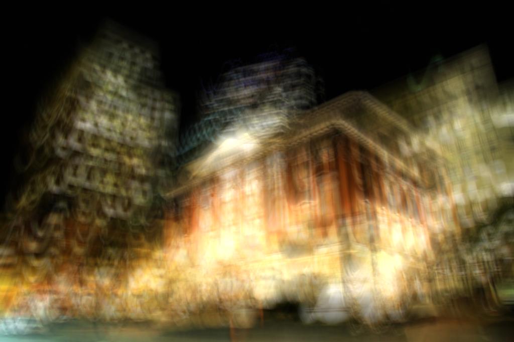
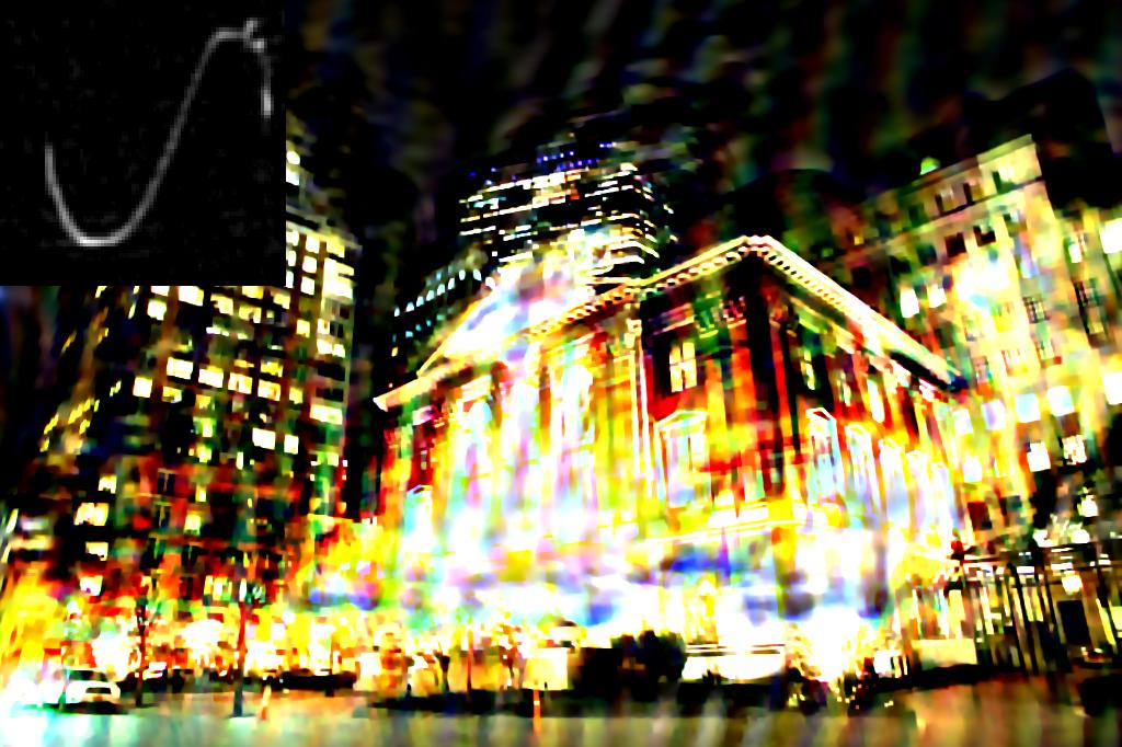
Blurry image	Xu & Jia [48]
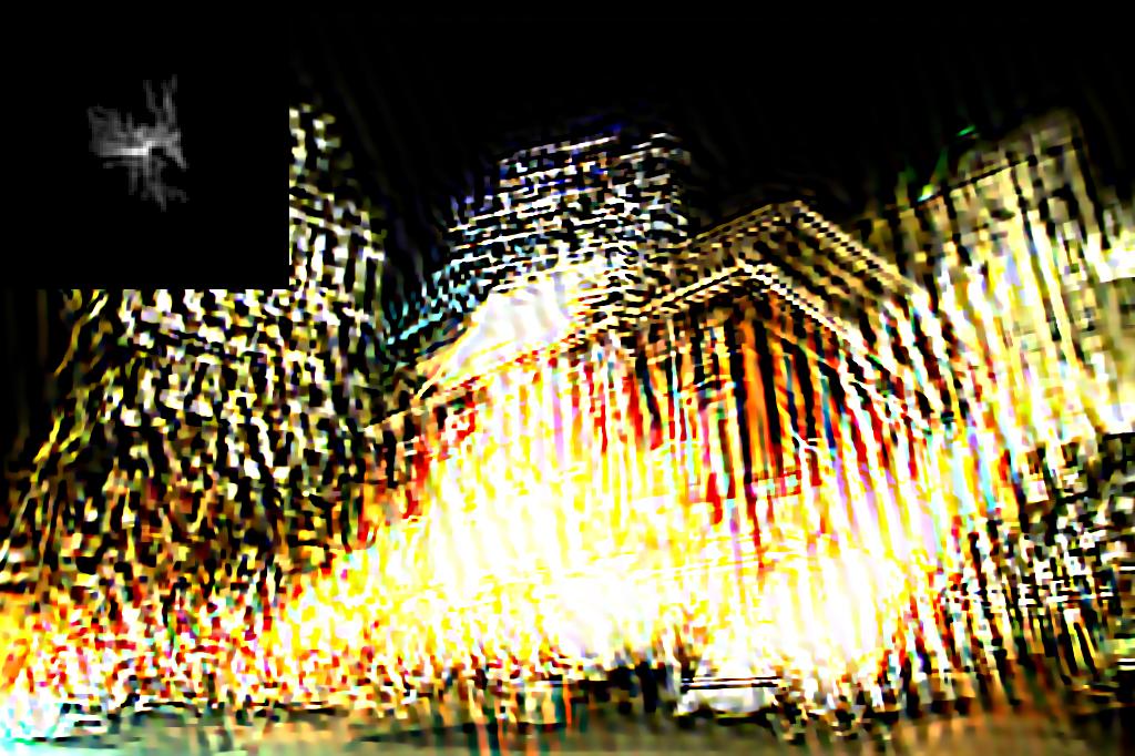
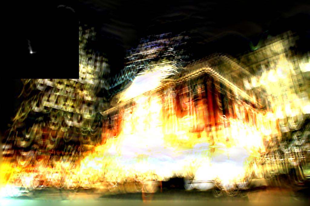
Pan-L0[27]	Sun et al. [41]
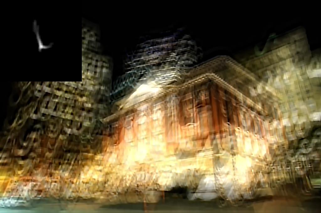
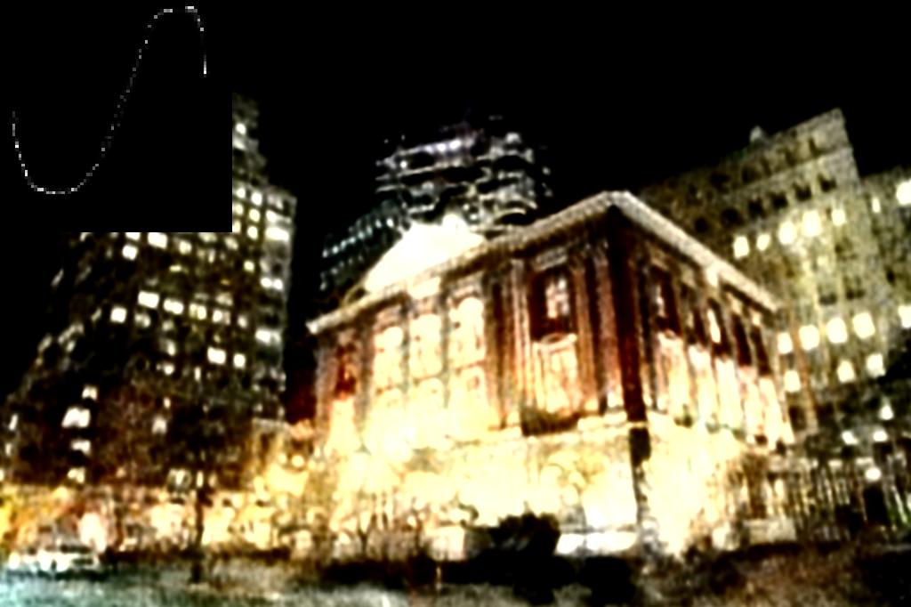
Pan-DCP[29]	SelfDeblur

Figure 1: Visual quality comparison on a severe blurry image.

Camera shake during exposure inevitably yields blurry images and is a long-standing annoying issue in digital photography. The removal of distortion from a blurry image, i.e., image deblurring, is a classical ill-posed problem in low-level vision and has received considerable research attention [2, 4, 19, 28, 56, 32, 29, 3, 10]. When the blur kernel is spatially invariant, it is also known as blind deconvolution, where the blurry image $\mathbf{y}$ can be formulated as,

$$\mathbf{y}=\mathbf{k}\otimes\mathbf{x}+\mathbf{n},$$ (1)

where $\otimes$ denotes the 2D convolution operator, $\mathbf{x}$ is the latent clean image, $\mathbf{k}$ is the blur kernel, and $\mathbf{n}$ is the additive white Gaussian noise (AWGN) with noise level $\sigma$. It can be seen that blind deconvolution should estimate both $\mathbf{k}$ and $\mathbf{x}$ from a blurry image $\bf y$, making it remain a very challenging problem after decades of studies.

Most traditional blind deconvolution methods are based on the Maximum a Posterior (MAP) framework,

$$\footnotesize\left(\mathbf{k},\mathbf{x}\right) =\arg\underset{\mathbf{x},\mathbf{k}}{\mathop{\max}}\,\Pr\left(\mathbf{k},\mathbf{x}|{\mathbf{y}}\right),$$ (2)

$$=\arg\underset{\mathbf{x},\mathbf{k}}{\mathop{\max}}\Pr\left({\mathbf{y}}|\mathbf{k},\mathbf{x}\right)\Pr\left(\mathbf{x}\right)\Pr\left(\mathbf{k}\right),$$

where $\Pr\left({\mathbf{y}}|\mathbf{k},\mathbf{x}\right)$ is the likelihood corresponding to the fidelity term, and $\Pr\left(\mathbf{x}\right)$ and $\Pr\left(\mathbf{k}\right)$ model the priors of clean image and blur kernel, respectively. Although many priors have been suggested for $\mathbf{x}$ [2, 27, 56, 15] and $\mathbf{k}$ [56, 29, 19, 22, 41, 24, 34, 29, 50], they generally are handcrafted and certainly are insufficient in characterizing clean images and blur kernels. Furthermore, the non-convexity of MAP based models also increases the difficulty of optimization. Levin et al. [19] reveal that MAP-based methods may converge to trivial solution of delta kernel. Perrone and Favaro [32] show that the success of existing methods can be attributed to some optimization details, e.g., projected alternating minimization and delayed normalization of $\mathbf{k}$.

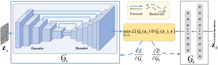
Figure 2: Illustration of our SelfDeblur method. The generative networks $\mathcal{G}_{x}$ and $\mathcal{G}_{k}$ are deployed to respectively capture the deep priors of blur kernel and latent clean image, and are trained using only the input blurry image. In particular, $\mathcal{G}_{x}$ is an asymmetric Autoencoder with skip connections, and the Sigmoid nonlinearity is adopted to the output layer for constraining the pixels in $\mathbf{x}$ in the range $[0,1]$. $\mathcal{G}_{k}$ adopts a fully-connected network, where the SoftMax nonlinearity is applied to the output layer for meeting the non-negative and equality constraints, and the 1D output of is reshaped to 2D blur kernel.

Motivated by the unprecedented success of deep learning in low-level vision [11, 52, 12, 42, 23], some attempts have also been made to solve blind deconvolution using deep convolutional neural networks (CNNs). Given the training set, deep CNNs can either be used to extract features to facilitate blur kernel estimation [38, 1], or be deployed to learn the direct mapping to clean image for motion deblurring [51, 25, 43, 7]. However, these methods do not succeed in handling various complex and large size blur kernels in blind deconvolution. Recently, Ulyanov et al. [45] suggest the deep image prior (DIP) framework, which adopts the structure of a DIP generator network to capture low-level image statistics and shows powerful ability in image denoising, super-resolution, inpainting, etc. Subsequently, Gandelsman et al. [6] combine multiple DIPs (i.e., Double-DIP) for multi-task layer decomposition such as image dehazing and transparency separation. However, Double-DIP cannot be directly applied to solve blind deconvolution due to that the DIP network is designed to generate natural images and is limited to capture the prior of blur kernels.

In this paper, we propose a novel neural optimization solution to blind deconvolution. Motivated by the DIP network [45], an image generator network $\mathcal{G}_{x}$, i.e., an asymmetric Autoencoder with skip connections, is deployed to capture the statistics of latent clean image. Nonetheless, image generator network cannot well characterize the prior on blur kernel. Instead, we adopt a fully-connected network (FCN) $\mathcal{G}_{k}$ to model the prior of blur kernel. Furthermore, the SoftMax nonlinearity is deployed to the output layer of $\mathcal{G}_{k}$, and the non-negative and equality constraints on blur kernel can then be naturally satisfied. By fixing the network structures ($\mathcal{G}_{k}$ and $\mathcal{G}_{x}$) and inputs ($\mathbf{z}_{k}$ and $\mathbf{z}_{x}$) sampled from uniform distribution, blind deconvolution is thus formulated as an unconstrained neural optimization on network parameters of $\mathcal{G}_{k}$ and $\mathcal{G}_{x}$. As illustrated in Fig. 2, given a blurry image $\bf y$, the optimization process can also be explained as a kind of “zero-shot” self-supervised learning [39] of $\mathcal{G}_{k}$ and $\mathcal{G}_{x}$, and our proposed method is dubbed SelfDeblur. Even though SelfDeblur can be optimized with either alternating optimization or joint optimization, our empirical study shows that the latter performs better in most cases.

Experiments are conducted on two widely used benchmarks [19, 18] as well as real-world blurry images to evaluate our SelfDeblur. Fig. 1 shows the deblurring results on a severe real-world blurry image. While the competing methods either fail to estimate large size blur kernels or suffer from ringing effects, our SelfDeblur succeed in estimating the blur kernel and generating visually favorable deblurring image. In comparison to the state-of-the-art methods, our SelfDeblur can achieve notable quantitative performance gains and performs favorably in generating visually plausible deblurring results. It is worth noting that our SelfDeblur can both estimate blur kernel and generate latent clean image with satisfying visual quality, making the subsequent non-blind deconvolution not a compulsory choice.

Our contributions are summarized as follows:

• A neural blind deconvolution method, i.e., SelfDeblur, is proposed, where DIP and FCN are respectively introduced to capture the priors of clean image and blur kernel. And the SoftMax nonlinearity is applied to the output layer of FCN to meet the non-negative and equality constraints.

• The joint optimization algorithm is suggested to solve the unconstrained neural blind deconvolution model for both estimating blur kernel and generating latent clean image, making the non-blind deconvolution not a compulsory choice for our SelfDeblur.

• Extensive experiments show that our SelfDeblur performs favorably against the existing MAP-based methods in terms of quantitative and qualitative evaluation. To our best knowledge, SelfDeblur makes the first attempt of applying deep learning to yield state-of-the-art blind deconvolution performance.

2 Related Work

In this section, we briefly survey the relevant works including optimization-based blind deconvolution and deep learning based blind deblurring methods.

2.1 Optimization-based Blind Deconvolution

Traditional optimization-based blind deconvolution methods can be further categorized into two groups, i.e., Variational Bayes (VB)-based and MAP-based methods. VB-based method [20] is theoretically promising, but is with heavy computational cost. As for the MAP-based methods, many priors have been suggested for modeling clean images and blur kernels. In the seminal work of [2], Chan et al. introduce the total variation (TV) regularization to model latent clean image in blind deconvolution, and motivates several variants based on gradient-based priors, e.g., $\ell_{0}$-norm [27] and $\ell_{p}$-norm [56]. Other specifically designed regularizations, e.g., $\ell_{1}/\ell_{2}$-norm [15], patch-based prior [41, 24], low-rank prior [34] and dark channel prior [29, 50] have also been proposed to identify and preserve salient edges for benefiting blur kernel estimation. Recently, a discriminative prior [21] is presented to distinguish the clean image from a blurry one, but still heavily relies on $\ell_{0}$-norm regularizer for attaining state-of-the-art performance. As for $\Pr(\mathbf{k})$, gradient sparsity priors [56, 29, 19] and spectral prior [22] are usually adopted. In order to solve the MAP-based model, several tricks have been introduced to the projected alternating minimization algorithm, including delayed normalization of blur kernel [32], multi-scale implementation [15] and time-varying parameters [56].

After blur kernel estimation, non-blind deconvolution is required to recover the latent clean image with fine texture details [15, 27, 29, 41, 49, 22]. Thus, the priors should favor natural images, e.g., hyper-Laplacian [14], GMM [55], non-local similarity [5], e.g., RTF [37], CSF [36] and CNN [16, 53], which are quite different from those used in blur kernel estimation. Our SelfDeblur can be regarded as a special MAP-based method, but two generative networks, i.e., DIP and FCN, are adopted to respectively capture the deep priors of clean image and blur kernel. Moreover, the joint optimization algorithm is effective to estimate blur kernel and generate clean image, making non-blind deconvolution not a compulsory choice for SelfDeblur.

2.2 Deep Learning in Image Deblurring

Many studies have been given to apply deep learning (DL) to blind deblurring. For example, DL can be used to help the learning of mapping to blur kernel. By imitating the alternating minimization steps in optimization-based methods, Schuler et al. [38] design the deep network architectures for blur kernel estimation. By studying the spectral property of blurry images, deep CNN is suggested to predict the Fourier coefficients [1], which can then be projected to estimate blur kernel. In [40], CNN is used to predict the parametric blur kernels for motion blurry images.

For dynamic scene deblurring, deep CNNs have been developed to learn the direct mapping to latent clean image [51, 25, 43, 40, 17]. Motivated by the multi-scale strategy in blind deconvolution, multi-scale CNN [25] and scale-recurrent network [43] are proposed to directly estimate the latent clean image from the blurry image. The adversarial loss is also introduced for better recovery of texture details in motion deblurring [17]. Besides, by exploiting the temporal information between adjacent frames, deep networks have also been applied to video motion deblurring [26, 9, 30]. However, due to the severe ill-posedness caused by large size and complex blur kernels, existing DL-based methods still cannot outperform traditional optimization-based ones for blind deconvolution.

Recently, DIP [45] and Double-DIP [6] have been introduced to capture image statistics, and have been deployed to many low-level vision tasks such as super-resolution, inpainting, dehazing, transparency separation, etc. Nonetheless, the DIP network is limited in capturing the prior of blur kernels, and Double-DIP still performs poorly for blind deconvolution. To the best of our knowledge, our SelfDeblur makes the first attempt of applying deep networks to yield state-of-the-art blind deconvolution performance.

3 Proposed Method

In this section, we first introduce the general formulation of MAP-based blind deconvolution, and then present our proposed neural blind deconvolution model as well as the joint optimization algorithm.

3.1 MAP-based Blind Deconvolution Formulation

According to Eqn. (1), we define the fidelity term as $-\log\left(\Pr\left({\mathbf{y}}|\mathbf{k},\mathbf{x}\right)\right)=\|\mathbf{k}\otimes\mathbf{x}-\mathbf{y}\|^{2}$. And we further introduce two regularization terms $-\log(\Pr(\mathbf{x}))=\phi(\mathbf{x})$ and $-\log(\Pr(\mathbf{k}))=\varphi(\mathbf{k})$ for modeling the priors on latent clean image and blur kernel, respectively. The MAP-based blind deconvolution model in Eqn. (2) can then be reformulated as,

$$( \mathbf{x},\mathbf{k})=\arg\underset{(\mathbf{x},\mathbf{k})}{\min}\|\mathbf{k}\otimes\mathbf{x}-\mathbf{y}\|^{2}+\lambda\phi(\mathbf{x})+\tau\varphi(\mathbf{k})$$ (3)

$${s.t.}\ 0\leq x_{i}\leq 1,\forall i,k_{j}\geq 0,\sum\nolimits_{j}{k_{j}}=1,\forall j,$$

where $\lambda$ and $\tau$ are trade-off regularization parameters. Besides the two regularization terms, we further introduce the non-negative and equality constraints for blur kernel $\mathbf{k}$ [41, 56, 29, 32], and the pixels in $\bf x$ are also constrained to the range $[0,1]$.

Under the MAP-based framework, many fixed and handcrafted regularization terms have been presented for latent clean image and blur kernel [56, 29, 22, 41, 24, 34, 29, 50]. To solve the model in Eqn. (3), projected alternating minimization is generally adopted, but several optimization details, e.g., delayed normalization [32] and multi-scale implementation [15], are also crucial to the success of blind deconvolution. Moreover, once the estimated blur kernel $\mathbf{\hat{k}}$ is obtained by solving Eqn. (3), another non-blind deconvolution usually is required to generate final deblurring result,

$$\mathbf{x}\!=\!\arg\underset{\mathbf{x}}{\min}\|\mathbf{\hat{k}}\otimes\mathbf{x}\!-\!\mathbf{y}\|^{2}\!+\!\lambda\mathcal{R}(\mathbf{x}),$$ (4)

where $\mathcal{R}(\mathbf{x})$ is a regularizer to capture natural image statistics and is quite different from $\phi(\mathbf{x})$.

3.2 Neural Blind Deconvolution

Motivated by the success of DIP [45] and Double-DIP [6], we suggest the neural blind deconvolution model by adopting generative networks $\mathcal{G}_{x}$ and $\mathcal{G}_{k}$ to capture the priors of $\bf x$ and $\bf k$. By substituting $\bf x$ and $\bf k$ with $\mathcal{G}_{x}$ and $\mathcal{G}_{k}$ and removing the regularization terms $\phi(\mathbf{x})$ and $\varphi(\mathbf{k})$, the neural blind deconvolution can be formulated as,

$$\underset{(\mathcal{G}_{x},\mathcal{G}_{k})}{\min}\|\mathcal{G}_{k}(\mathbf{z}_{k})\otimes\mathcal{G}_{x}(\mathbf{z}_{x})-\mathbf{y}\|^{2}$$ (5)

$$s.t.\ \ 0\leq(\mathcal{G}_{x}(\mathbf{z}_{x}))_{i}\leq 1,\forall i,$$

$$\ \ \ \ \ \ \ (\mathcal{G}_{k}(\mathbf{z}_{k}))_{j}\geq 0,\sum\nolimits_{j}{(\mathcal{G}_{k}(\mathbf{z}_{k}))_{j}}=1,\forall j,$$

where $\mathbf{z}_{x}$ and $\mathbf{z}_{k}$ are sampled from the uniform distribution, $(\cdot)_{i}$ and $(\cdot)_{j}$ denote the $i$-th and $j$-th elements. We note that $\mathbf{z}_{k}$ is 1D vector, and $\mathcal{G}_{k}(\mathbf{z}_{k})$ is reshaped to obtain 2D matrix of blur kernel.

However, there remain several issues to be addressed with neural blind deconvolution. (i) The DIP network [45] is designed to capture low-level image statistics and is limited in capturing the prior of blur kernels. As a result, we empirically find that Double-DIP [6] performs poorly for blind deconvolution (see the results in Sec. 4.1.2). (ii) Due to the non-negative and equality constraints, the resulting model in Eqn. (5) is a constrained neural optimization problem and is difficult to optimize. (iii) Although the generative networks $\mathcal{G}_{x}$ and $\mathcal{G}_{k}$ present high impedance to image noise, the denoising performance of DIP heavily relies on the additional averaging over last iterations and different optimization runs [45]. Such heuristic solutions, however, both bring more computational cost and cannot be directly borrowed to handle blurry and noisy images.

In the following, we present our solution to address the issues (i)&(ii) by designing proper generative networks $\mathcal{G}_{x}$ and $\mathcal{G}_{k}$. As for the issue (iii), we introduce an extra TV regularizer and a regularization parameter to explicitly consider noise level in the neural blind deconvolution model.

Generative Network $\mathcal{G}_{x}$. The latent clean images usually contain salient structures and rich textures, which requires the generative network $\mathcal{G}_{x}$ to have sufficient modeling capacity. Fortunately, since the introduction of generative adversarial network [8], dramatic progress has been made in generating high quality natural images [45]. For modeling $\mathbf{x}$, we adopt a DIP network, i.e., the asymmetric Autoencoder [35] with skip connections in [45], to serve as $\mathcal{G}_{x}$. As shown in Fig. 2, the first 5 layers of encoder are skip connected to the last 5 layers of decoder. Finally, a convolutional output layer is used to generate latent clean image. To meet the range constraint for $\mathbf{x}$, the Sigmoid nonlinearity is applied to the output layer. Please refer to the supplementary file for more architecture details of $\mathcal{G}_{x}$.

Generative Network $\mathcal{G}_{k}$. On the one hand, the DIP network [45] is designed to capture the statistics of natural image but performs limited in modeling the prior of blur kernel. On the other hand, blur kernel $\mathbf{k}$ generally contains much fewer information than latent clean image $\mathbf{x}$, and can be well generated by simpler generative network. Thus, we simply adopt a fully-connected network (FCN) to serve as $\mathcal{G}_{k}$. As shown in Fig. 2, the FCN $\mathcal{G}_{k}$ takes a 1D noise $\mathbf{z}_{k}$ with 200 dimensions as input, and has a hidden layer of 1,000 nodes and an output layer of $K^{2}$ nodes. To guarantee the non-negative and equalitly constraints can be always satisfied, the SoftMax nonlinearity is applied to the output layer of $\mathcal{G}_{k}$. Finally, the 1D output of $K^{2}$ entries is reshaped to a 2D $K\times K$ blur kernel. Please refer to Suppl. for more architecture details of $\mathcal{G}_{k}$.

Unconstrained Neural Blind Deconvolution with TV Regularization. With the above generative networks $\mathcal{G}_{x}$ and $\mathcal{G}_{k}$, we can formulate neural blind deconvolution into an unconstrained optimization form. However, the resulting model is irrelevant with the noise level, making it perform poorly on blurry images with non-negligible noise. To address this issue, we combine both $\mathcal{G}_{x}$ and TV regularization to capture image priors, and our neural blind deconvolution model can then be written as,

$$\underset{\mathcal{G}_{k},\mathcal{G}_{x}}{\min}\|\mathcal{G}_{k}(\mathbf{z}_{k})\otimes\mathcal{G}_{x}(\mathbf{z}_{x})\!-\!\mathbf{y}\|^{2}\!+\!\lambda\text{TV}(\mathcal{G}_{x}(\mathbf{z}_{x})),$$ (6)

where $\lambda$ denotes the regularization parameter controlled by noise level $\sigma$. Albeit the generative network $\mathcal{G}_{x}$ is more powerful, the incorporation of $\mathcal{G}_{x}$ and another image prior generally is beneficial to deconvolution performance. Moreover, the introduction of the noise level related regularization parameter $\lambda$ can greatly improve the robustness in handling blurry images with various noise levels. In particular, we emperically set $\lambda=0.1\times\sigma$ in our implementation, and the noise level $\sigma$ can be estimated using [54].

3.3 Optimization Algorithm

The optimization process of Eqn. (6) can be explained as a kind of ”zero-shot” self-supervised learning [39], where the generative networks $\mathcal{G}_{k}$ and $\mathcal{G}_{x}$ are trained using only a test image (i.e., blurry image $\bf y$) and no ground-truth clean image is available. Thus, our method is dubbed SelfDeblur. In the following, we present two algorithms for SelfDeblur, i.e., alternating optimization and joint optimization.

Alternating Optimization. Analogous to the alternating minimization steps in traditional blind deconvolution [56, 2, 29, 27, 41], the network parameters of $\mathcal{G}_{k}$ and $\mathcal{G}_{x}$ can also be optimized in an alternating manner. As summarized in Algorithm 1, the parameters of $\mathcal{G}_{k}$ are updated via the ADAM [13] by fixing $\mathcal{G}_{x}$, and vice versa. In particular, the gradient w.r.t. either $\mathcal{G}_{x}$ or $\mathcal{G}_{k}$ can be derived using automatic differentiation [31].

Joint Optimization. In traditional MAP-based framework, alternating minimization allows the use of projection operator to handle non-negative and equality constraints and the modification of optimization details to avoid trivial solution, and thus has been widely adopted. As for our neural blind deconvolution, the model in Eqn. (6) is unconstrained optimization, and the powerful modeling capacity of $\mathcal{G}_{k}$ and $\mathcal{G}_{x}$ is beneficial to avoid trivial delta kernel solution. We also note that the unconstrained neural blind deconvolution is highly non-convex, and alternating optimization may get stuck at saddle points [44]. Thus, joint optimization is more prefered than alternating optimization for SelfDeblur. Using the automatic differentiation techniques [31], the gradients w.r.t. $\mathcal{G}_{k}$ and $\mathcal{G}_{x}$ can be derived. Algorithm 2 summarizes the joint optimization algorithm, where the parameters of $\mathcal{G}_{k}$ and $\mathcal{G}_{x}$ can be jointly updated using the ADAM algorithm. Our empirical study in Sec. 4.1.1 also shows that joint optimization usually converges to better solutions than alternating optimization.

Both alternating optimization and joint optimization algorithms are stopped when reaching $T$ iterations. Then, the estimated blur kernel and latent clean image can be generated using $\mathbf{k}=\mathcal{G}^{T}_{k}(\mathbf{z}_{k})$ and $\mathbf{x}=\mathcal{G}^{T}_{x}(\mathbf{z}_{x})$, respectively. Benefited from the modeling capacity of $\mathcal{G}_{x}(\mathbf{z}_{x})$, the estimated $\bf x$ is with visually favorable textures, and it is not a compulsory choice for our SelfDeblur to adopt another non-blind deconvolution method to generate final deblurring result.

Algorithm 1 SelfDeblur (Alternating Optimization)

1:Blurry image $\mathbf{y}$

2:Blur kernel $\mathbf{k}$ and clean image $\mathbf{x}$

3:Sample $\mathbf{z}_{x}$ and $\mathbf{z}_{k}$ from uniform distribution with seed 0.

4:$\mathbf{k}=\mathcal{G}_{k}^{0}(\mathbf{z}_{k})$

5:for $t=1\text{ to }T$ do

6:    $\mathbf{x}=\mathcal{G}^{t-1}_{x}(\mathbf{z}_{x})$

7:    Compute the gradient w.r.t. $\mathcal{G}_{k}$

8:    Update $\mathcal{G}_{k}^{t}$ using the ADAM algorithm [13]

9:    $\mathbf{k}=\mathcal{G}^{t}_{k}(\mathbf{z}_{k})$

10:    Compute the gradient w.r.t. $\mathcal{G}_{x}$

11:    Update $\mathcal{G}_{x}^{t}$ using the ADAM algorithm [13]

12:end for

13:$\mathbf{x}=\mathcal{G}^{T}_{x}(\mathbf{z}_{x})$, $\mathbf{k}=\mathcal{G}^{T}_{x}(\mathbf{z}_{k})$

Algorithm 2 SelfDeblur (Joint Optimization)

1:Blurry image $\mathbf{y}$

2:Blur kernel $\mathbf{k}$ and clean image $\mathbf{x}$

3:Sample $\mathbf{z}_{x}$ and $\mathbf{z}_{k}$ from uniform distribution with seed 0.

4:for $t=1\text{ to }T$ do

5:    $\mathbf{k}=\mathcal{G}^{t-1}_{k}(\mathbf{z}_{k})$

6:    $\mathbf{x}=\mathcal{G}_{x}^{t-1}(\mathbf{z}_{x})$

7:    Compute the gradients w.r.t. $\mathcal{G}_{k}$ and $\mathcal{G}_{x}$

8:    Update $\mathcal{G}_{k}^{t}$ and $\mathcal{G}_{x}^{t}$ using the ADAM algorithm [13]

9:end for

10:$\mathbf{x}=\mathcal{G}^{T}_{x}(\mathbf{z}_{x})$, $\mathbf{k}=\mathcal{G}^{T}_{x}(\mathbf{z}_{k})$

4 Experimental Results

In this section, ablation study is first conducted to analyze the effect of optimization algorithm and network architecture. Then, our SelfDeblur is evaluated on two benchmark datasets and is compared with the state-of-the-art blind deconvolution methods. Finally, we report the results of SelfDeblur on several real-world blurry images.

Our SelfDeblur is implemented using Pytorch [31]. The experiments are conducted on a PC equipped with one NVIDIA Titan V GPU. Unless specially stated, the experiments follow the same settings, i.e., $T=5,000$, and the noises $\mathbf{z}_{x}$ and $\mathbf{z}_{k}$ are sampled from the uniform distribution with fixed random seed 0. Following [45], we further perturb $\mathbf{z}_{x}$ randomly at each iteration. The initial learning rate is set as $0.01$ and is decayed by multiplying 0.5 when reaching 2,000, 3,000 and 4,000 iterations.

​​​​​

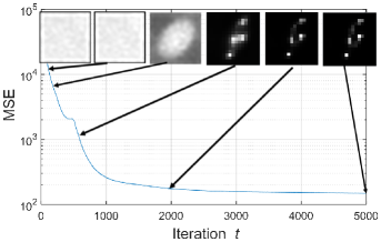
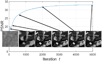
Figure 3: Intermediate results of estimated blur kernel and latent clean image at iteration $t=1,20,100,600,2,000\text{ and }5,000$.

4.1 Ablation Study

Ablation study is conducted on the dataset by Levin et al. [19], which is a popular blind deconvolution benchmark consisting of 4 clean images and 8 blur kernels. Using [54], the average estimated noise level of the blurry images in the dataset is $\sigma\approx 1\times 10^{-5}$. Thus we simply adopt $\lambda=1\times 10^{-6}$ on this dataset.

4.1.1 Alternating Optimization vs. Joint Optimization

We first evaluate the performance of SelfDeblur using alternating optimization (SelfDeblur-A) and joint optimization (SelfDeblur-J). Table 1 reports the average PSNR and SSIM values. In terms of quantitative metrics, SelfDeblur-J significantly outperforms SelfDeblur-A, demonstrating the superiority of joint optimization. In the supplementary file, we provide several failure cases of SelfDeblur-A, where SelfDeblur-A may converge to delta kernel and worse solution while SelfDeblur-J performs favorably on these cases. Therefore, joint optimization is adopted as the default SelfDeblur method throughout the following experiments.

Table 1: Average PSNR/SSIM comparison of SelfDeblur-A and SelfDeblur-J on the dataset of Levin et al. [19].

SelfDeblur-A	SelfDeblur-J
30.53 / 0.8748	33.07 / 0.9313

4.1.2 Network Architecture of $\mathcal{G}_{k}$

In this experiment, we compare the results by considering four kinds of network architectures: (i) SelfDeblur, (ii) Double-DIP [6] (asymmetric Autoencoder with skip connections for both $\mathcal{G}_{x}$ and $\mathcal{G}_{k}$), (iii) SelfDeblur_k- (removing the hidden layer from $\mathcal{G}_{k}$), and (iv) SelfDeblur_k+ (adding an extra hidden layer for $\mathcal{G}_{k}$). From Table 2 and Fig. 4, SelfDeblur significantly outperforms Double-DIP in estimating blur kernel and latent image. The result indicates that the DIP network is limited to capture the prior of blur kernel, and the simple FCN can be a good choice of $\mathcal{G}_{k}$. We further compare SelfDeblur with SelfDeblur_k- and SelfDeblur_k+. One can see that the FCN without hidden layer (i.e., SelfDeblur_k-) also succeeds in estimating blur kernel and clean image (see Fig. 4), but performs much inferior to SelfDeblur. Moreover, the three-layer FCN (i.e., SelfDeblur_k+) is superior to SelfDeblur_k-, but is inferior to SelfDeblur. To sum up, SelfDeblur is a good choice for modeling blur kernel prior.

Table 2: Quantitavie comparison of SelfDeblur variants with different network structures of $\mathcal{G}_{k}$.

	SelfDeblur	SelfDeblurk-	SelfDeblurk+	Double-DIP
PSNR	33.07	28.37	30.92	21.51
SSIM	0.9313	0.8396	0.8889	0.5256

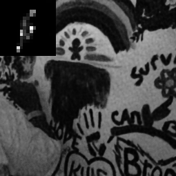
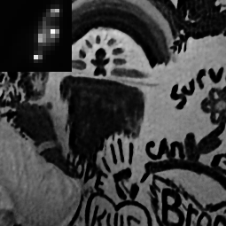
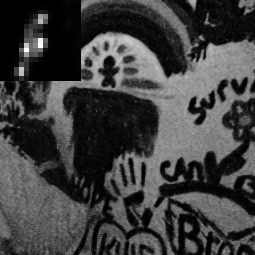
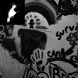
SelfDeblur	SelfDeblurk-	SelfDeblurk+	Double-DIP

Figure 4: Visual comparison of SelfDeblur variants with different network structures of $\mathcal{G}_{k}$.

4.1.3 Visualization of Intermediate Results

Using an image from the dataset of Levin et al. [19], Fig. 3 shows the intermediate results of estimated blur kernel and clean image at iteration $t$ $=$ $1,20,100,600,2,000\text{ and }5,000$, along with the MSE curve for $\bf k$ and the PSNR curve for $\bf x$. When iteration $t=20$, the intermediate result of $\bf x$ mainly contains the salient image structures, which is consistent with the observation that salient edges is crucial for initial blur kernel estimation in traditional methods. Along with the increase of iterations, $\mathcal{G}_{x}$ and $\mathcal{G}_{k}$ begin to generate finer details in $\bf x$ and $\bf k$. Unlike traditional methods, SelfDeblur is effective in simultaneously estimating blur kernel and recovering latent clean image when iteration $t\geq 20$, making the non-blind deconvolution not a compulsory choice for SelfDeblur.

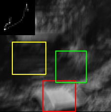
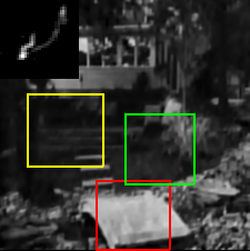
Blurry image			Zuo et al. Δ[56]			Xu&JiaΔ[48]			SelfDeblurΔ
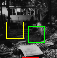
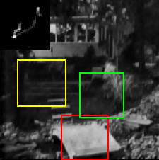
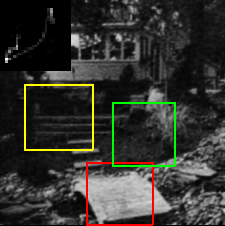
Ground-truth			Sun et al. Δ[41]			Pan-DCPΔ[29]			SelfDeblur

Figure 5: Visual comparison on the dataset of Levin et al. [19].

4.2 Comparison with State-of-the-arts

4.2.1 Results on dataset of Levin et al. [19]

Table 3: Average PSNR, SSIM, Error Ratio and running time (sec.) comparison on the dataset of Levin et al. [19]. ^Δ indicates the method generates final deblurring results using the non-blind deconvolution method from [20]. The running time only includes blur kernel estimation.

	PSNR	SSIM	Error Ratio	Time
Known kΔ	34.53	0.9492	1.0000	—
Krishnan et al. Δ [15]	29.88	0.8666	2.4523	8.9400
Cho&LeeΔ [4]	30.57	0.8966	1.7113	1.3951
Levin et al. Δ [20]	30.80	0.9092	1.7724	78.263
Xu&JiaΔ [49]	31.67	0.9163	1.4898	1.1840
Sun et al. Δ [41]	32.99	0.9330	1.2847	191.03
Zuo et al. Δ [56]	32.66	0.9332	1.2500	10.998
Pan-DCPΔ [29]	32.69	0.9284	1.2555	295.23
SRN[43]	23.43	0.7117	6.0864	N/A
SelfDeblurΔ	33.32	0.9438	1.2509	—
SelfDeblur	33.07	0.9313	1.1968	224.01

Table 4: Average PSNR/SSIM comparison on the dataset of Lai et al. [18], which has 5 categories. The methods marked with ^Δ adopt [47] and [14] as non-blind deconvolution after blur kernel estimation in Saturated and the other categories, respectively.

Images	Cho&LeeΔ[4]	Xu&JiaΔ[48]	Xu et al. Δ[49]	Michaeli et al. Δ[24]	Perroe et al. Δ [32]	Pan-L0Δ[27]	Pan-DCPΔ[29]	SelfDeblurΔ	SelfDeblur
Manmade	16.35/0.3890	19.23/0.6540	17.99/0.5986	17.43/0.4189	17.41/0.5507	16.92/0.5316	18.59/0.5942	20.08/0.7338	20.35/0.7543
Natural	20.14/0.5198	23.03/0.7542	21.58/0.6788	20.70/0.5116	21.04/0.6764	20.92/0.6622	22.60/0.6984	22.50/0.7183	22.05/0.7092
People	19.90/0.5560	25.32/0.8517	24.40/0.8133	23.35/0.6999	22.77/0.7347	23.36/0.7822	24.03/0.7719	27.41/0.8784	25.94/0.8834
Saturated	14.05/0.4927	14.79/0.5632	14.53/0.5383	14.14/0.4914	14.24/0.5107	14.62/0.5451	16.52/0.6322	16.58/0.6165	16.35/0.6364
Text	14.87/0.4429	18.56/0.7171	17.64/0.6677	16.23/0.4686	16.94/0.5927	16.87/0.6030	17.42/0.6193	19.06/0.7126	20.16/0.7785
Avg.	17.06/0.4801	20.18/0.7080	19.23/0.6593	18.37/0.5181	18.48/0.6130	18.54/0.6248	19.89/0.6656	21.13/0.7319	20.97/0.7524

Using the dataset of Levin et al. [19], we compare our SelfDeblur with several state-of-the-art blind deconvolution methods, including Krishnan et al. [15], Levin et al. [19], Cho&Lee [4], Xu&Jia [48], Sun et al. [41], Zuo et al. [56] and Pan-DCP [29]. Besides, SelfDeblur is compared with one state-of-the-art deep motion deblurring method SRN [43], which is re-trained on 1,600 blurry images [33] synthesized using eight blur kernels in the dataset of Levin et al. For SelfDeblur, $\lambda=1\times 10^{-6}$ is set for all the blurry images. Following [41, 56], we adopt the non-blind deconvolution method in [20] to generate final deblurring results. PSNR, SSIM [46] and Error Ratio [20] are used as quantitative metrics. And we also report the running time of blur kernel estimation for each competing method. Our SelfDeblur and SRN are ran on an NVIDIA Titan V GPU, while the other methods are ran on a PC with 3.30GHz Intel(R) Xeon(R) CPU.

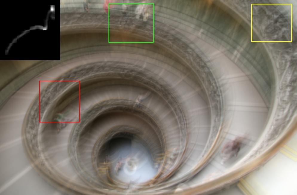
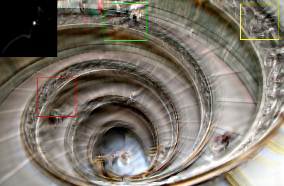
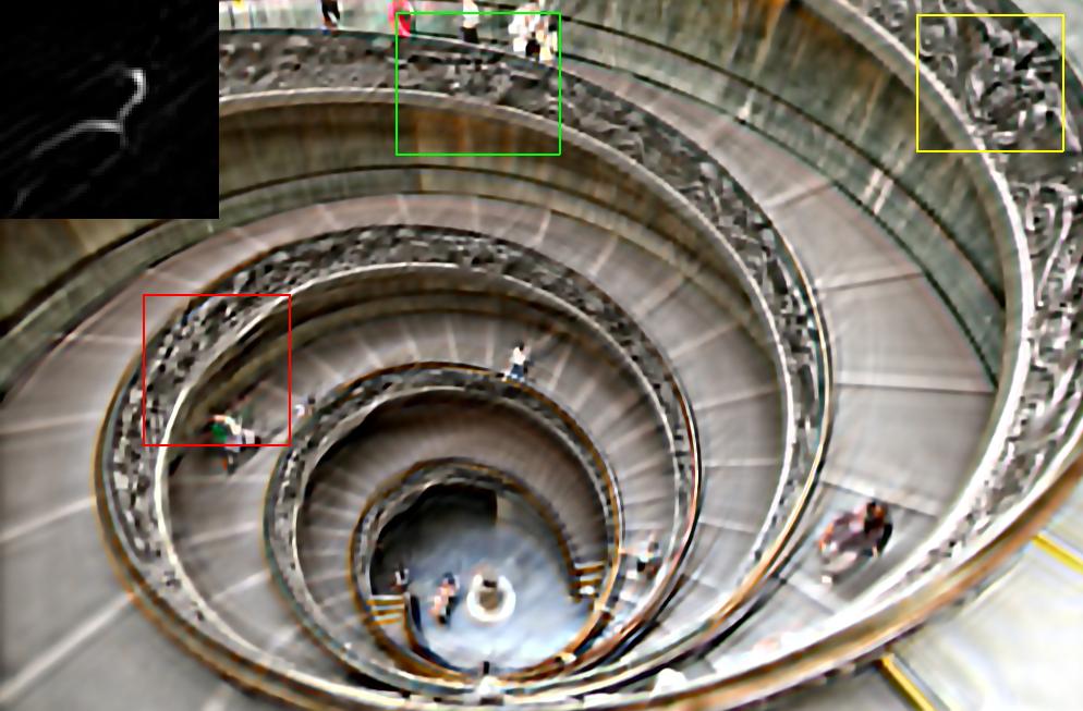
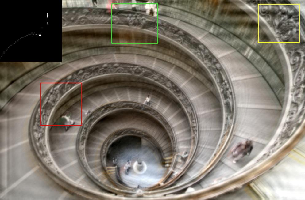
Blurry image			Xu&JiaΔ[48]			Perrone et al. Δ[32]			SelfDeblurΔ
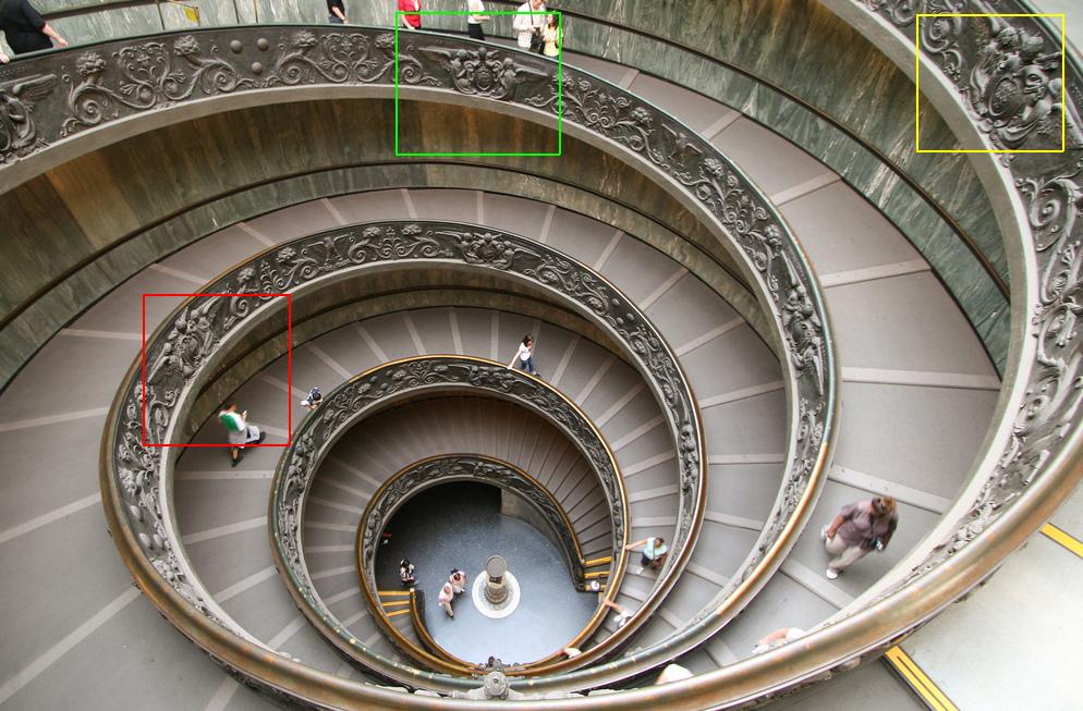
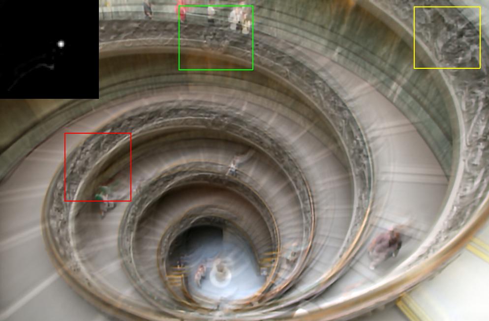
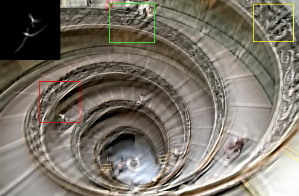
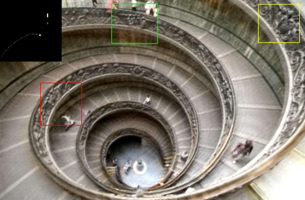
Ground-truth			Michaeli et al. Δ[48]			Pan-DCPΔ[32]			SelfDeblur

Figure 6: Visual comparison on the dataset of Lai et al. [18].

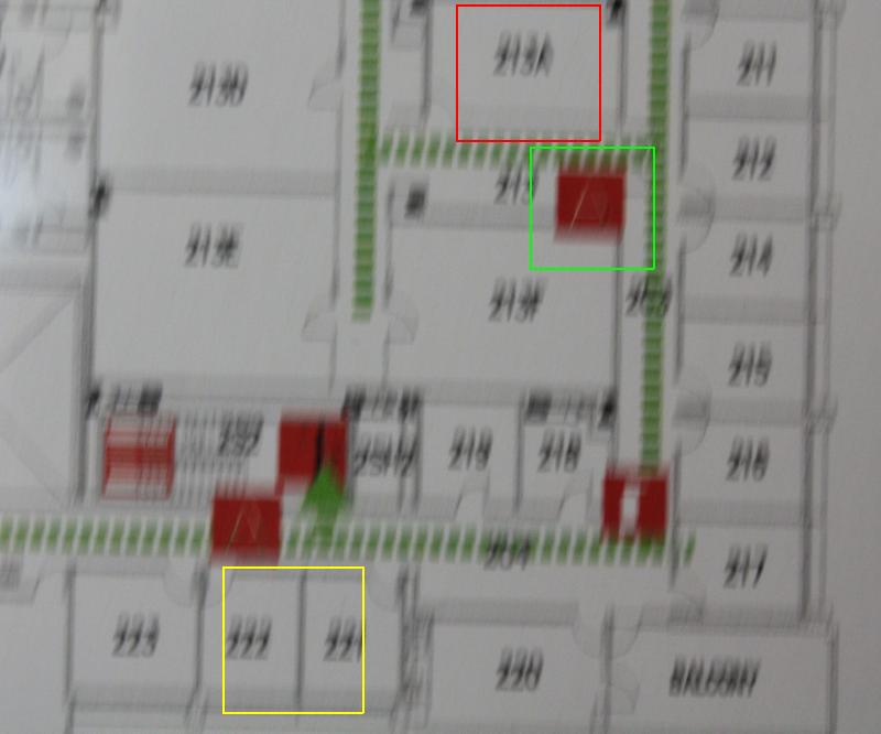
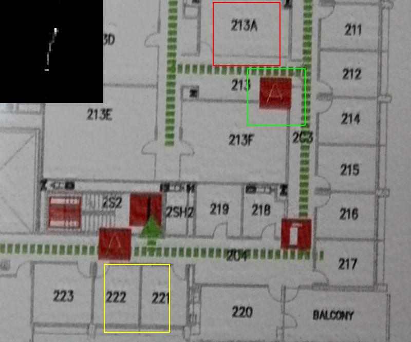
Blurry image			Xu&Jia[48]			Pan-DCP[29]			SelfDeblur

Figure 7: Visual comparison on two real-world blurry images.

Table 3 lists the average metrics of the competing methods. We report the results of SelfDeblur with two settings, i.e., the deblurring results purely by SelfDeblur and those using the non-blind deconvolution from [20], denoted as SelfDeblur^Δ. In terms of PSNR and Error Ratio, SelfDeblur significantly outperforms the competing methods. As for average SSIM, SelfDeblur performs slightly inferior to Sun et al. and Zuo et al. By incorporating with non-blind deconvolution from [20], SelfDeblur^Δ can further boost quantitative performance and outperforms all the other methods. In terms of running time, SelfDeblur is time-consuming due to the optimization of two generative networks, but is comparable with Sun et al. [41] and Pan-DCP [29]. From the visual comparison in Fig. 5, the #4 blur kernel estimated by SelfDeblur is much closer to the ground-truth. As shown in the close-ups, SelfDeblur and SelfDeblur^Δ can recover more visually favorable textures. We also note that both the performance gap and visual quality between SelfDeblur and SelfDeblur^Δ are not significant, and thus non-blind deconvolution is not a compulsory choice for our SelfDeblur.

4.2.2 Results on dataset of Lai et al. [18]

We further evaluate SelfDeblur on the dataset of Lai et al. [18] consisting of 25 clean images and 4 large size blur kernels. The blurry images are divided into five categories, i.e., Manmade, Natural, People, Saturated and Text, where each category contains 20 blurry images. For each blurry image, the parameter $\lambda$ is set according to the noise level estimated using [54]. We compare our SelfDeblur with Cho&Lee [4], Xu&Jia[48], Xu et al. [49], Machaeli et al. [24], Perroe et al. [32], Pan-L$0$ [27] and Pan-DCP [29]. The results of competing methods except Pan-DCP [29] and ours are duplicated from [18]. The results of Pan-DCP [29] are generated using their default settings. Once the blur kernel is estimated, non-blind deconvolution [14] is applied to the images of Manmade, Natural, People and Text, while [47] is used to handle Saturated images. From Table 4, both SelfDeblur and SelfDeblur^Δ can achieve better quantitative metrics than the competing methods. In terms of image contents, our SelfDeblur outperforms the other methods on any of the five categories. From the results in Fig. 6, the blur kernel estimated by our SelfDeblur is more accurate than those by the competing methods, and the deconvolution result is with more visually plausible textures.

4.3 Evaluation on Real-world Blurry Images

Our SelfDeblur is further compared with Xu&Jia [48] and Pan-DCP [29] on real-world blurry images. From Fig. 7, one can see that the blur kernel estimated by our SelfDeblur contains less noises, and the estimated clean image is with more visually plausible structures and textures. The kernel estimation errors by Xu&Jia and Pan-DCP are obvious, thereby yielding ringing artifacts in the estimated clean images. More results can be found in Suppl.

5 Conclusion

In this paper, we proposed a neural blind deconvolution method, i.e., SelfDeblur. It adopts an asymmetric Autoencoder and a FCN to respectively capture the deep priors of latent clean image and blur kernel. And the SoftMax nonlinearity is applied to the output of FCN to meet the non-negative and equality constraints of blur kernel. A joint optimization algorithm is suggested to solve the unconstrained neural blind deconvolution model. Experiments show that our SelfDeblur achieves notable performance gains over the state-of-the-art methods, and is effective in estimating blur kernel and generating clean image with visually favorable textures.

References

- [1] A. Chakrabarti. A neural approach to blind motion deblurring. In European Conference on Computer Vision, pages 221–235, 2016.
- [2] T. F. Chan and C.-K. Wong. Total variation blind deconvolution. IEEE Transactions on Image Processing, 7(3):370–375, 1998.
- [3] L. Chen, F. Fang, T. Wang, and G. Zhang. Blind image deblurring with local maximum gradient prior. In Proceedings of the IEEE Conference on Computer Vision and Pattern Recognition, pages 1742–1750, 2019.
- [4] S. Cho and S. Lee. Fast motion deblurring. ACM Transactions on Graphics, 28(5):145, 2009.
- [5] W. Dong, L. Zhang, G. Shi, and X. Li. Nonlocally centralized sparse representation for image restoration. IEEE Transactions on Image Processing, 22(4):1620–1630, 2013.
- [6] Y. Gandelsman, A. Shocher, and M. Irani. ” double-dip”: Unsupervised image decomposition via coupled deep-image-priors. In Proceedings of the IEEE Conference on Computer Vision and Pattern Recognition, 2019.
- [7] H. Gao, X. Tao, X. Shen, and J. Jia. Dynamic scene deblurring with parameter selective sharing and nested skip connections. In Proceedings of the IEEE Conference on Computer Vision and Pattern Recognition, pages 3848–3856, 2019.
- [8] I. Goodfellow, J. Pouget-Abadie, M. Mirza, B. Xu, D. Warde-Farley, S. Ozair, A. Courville, and Y. Bengio. Generative adversarial nets. In Advances in Neural Information Processing Systems, pages 2672–2680, 2014.
- [9] T. Hyun Kim, K. Mu Lee, B. Scholkopf, and M. Hirsch. Online video deblurring via dynamic temporal blending network. In Proceedings of the IEEE International Conference on Computer Vision, pages 4038–4047, 2017.
- [10] M. Jin, S. Roth, and P. Favaro. Normalized blind deconvolution. In European Conference on Computer Vision, 2018.
- [11] J. Kim, J. Kwon Lee, and K. Mu Lee. Accurate image super-resolution using very deep convolutional networks. In Proceedings of the IEEE Conference on Computer Vision and Pattern Recognition, pages 1646–1654, 2016.
- [12] J. Kim, J. Kwon Lee, and K. Mu Lee. Deeply-recursive convolutional network for image super-resolution. In Proceedings of the IEEE Conference on Computer Vision and Pattern Recognition, pages 1637–1645, 2016.
- [13] D. P. Kingma and J. Ba. Adam: A method for stochastic optimization. In International Conference on Learning Representation, 2015.
- [14] D. Krishnan and R. Fergus. Fast image deconvolution using hyper-Laplacian priors. In Advances in Neural Information Processing Systems, pages 1033–1041, 2009.
- [15] D. Krishnan, T. Tay, and R. Fergus. Blind deconvolution using a normalized sparsity measure. In Proceedings of the IEEE Conference on Computer Vision and Pattern Recognition, pages 233–240, 2011.
- [16] J. Kruse, C. Rother, and U. Schmidt. Learning to push the limits of efficient fft-based image deconvolution. In Proceedings of the IEEE International Conference on Computer Vision, pages 4586–4594, 2017.
- [17] O. Kupyn, V. Budzan, M. Mykhailych, D. Mishkin, and J. Matas. Deblurgan: Blind motion deblurring using conditional adversarial networks. In Proceedings of the IEEE Conference on Computer Vision and Pattern Recognition, pages 8183–8192, 2018.
- [18] W.-S. Lai, J.-B. Huang, Z. Hu, N. Ahuja, and M.-H. Yang. A comparative study for single image blind deblurring. In Proceedings of the IEEE Conference on Computer Vision and Pattern Recognition, pages 1701–1709, 2016.
- [19] A. Levin, Y. Weiss, F. Durand, and W. T. Freeman. Understanding and evaluating blind deconvolution algorithms. In Proceedings of the IEEE Conference on Computer Vision and Pattern Recognition, pages 1964–1971, 2009.
- [20] A. Levin, Y. Weiss, F. Durand, and W. T. Freeman. Efficient marginal likelihood optimization in blind deconvolution. In Proceedings of the IEEE Conference on Computer Vision and Pattern Recognition, pages 2657–2664, 2011.
- [21] L. Li, J. Pan, W.-S. Lai, C. Gao, N. Sang, and M.-H. Yang. Learning a discriminative prior for blind image deblurring. In Proceedings of the IEEE Conference on Computer Vision and Pattern Recognition, pages 6616–6625, 2018.
- [22] G. Liu, S. Chang, and Y. Ma. Blind image deblurring using spectral properties of convolution operators. IEEE Transactions on Image Processing, 23(12):5047–5056, 2014.
- [23] R. Liu, S. Cheng, Y. He, X. Fan, Z. Lin, and Z. Luo. On the convergence of learning-based iterative methods for nonconvex inverse problems. IEEE Transactions on Pattern Analysis and Machine Intelligence, 2019.
- [24] T. Michaeli and M. Irani. Blind deblurring using internal patch recurrence. In European Conference on Computer Vision, pages 783–798, 2014.
- [25] S. Nah, T. Hyun Kim, and K. Mu Lee. Deep multi-scale convolutional neural network for dynamic scene deblurring. In Proceedings of the IEEE Conference on Computer Vision and Pattern Recognition, pages 3883–3891, 2017.
- [26] S. Nah, S. Son, and K. M. Lee. Recurrent neural networks with intra-frame iterations for video deblurring. In Proceedings of the IEEE Conference on Computer Vision and Pattern Recognition, pages 8102–8111, 2019.
- [27] J. Pan, Z. Hu, Z. Su, and M.-H. Yang. -regularized intensity and gradient prior for deblurring text images and beyond. IEEE Transactions on Pattern Analysis and Machine Intelligence, 39(2):342–355, 2017.
- [28] J. Pan, W. Ren, Z. Hu, and M.-H. Yang. Learning to deblur images with exemplars. IEEE Transactions on Pattern Analysis and Machine Intelligence, 2018.
- [29] J. Pan, D. Sun, H. Pfister, and M.-H. Yang. Deblurring images via dark channel prior. IEEE Transactions on Pattern Analysis and Machine Intelligence, 40(10):2315–2328, 2018.
- [30] L. Pan, Y. Dai, M. Liu, and F. Porikli. Simultaneous stereo video deblurring and scene flow estimation. In Proceedings of the IEEE Conference on Computer Vision and Pattern Recognition, pages 4382–4391, 2017.
- [31] A. Paszke, S. Gross, S. Chintala, G. Chanan, E. Yang, Z. DeVito, Z. Lin, A. Desmaison, L. Antiga, and A. Lerer. Automatic differentiation in pytorch. In NIPS Autodiff Workshop: The Future of Gradient-based Machine Learning Software and Techniques, 2017.
- [32] D. Perrone and P. Favaro. Total variation blind deconvolution: The devil is in the details. In Proceedings of the IEEE Conference on Computer Vision and Pattern Recognition, pages 2909–2916, 2014.
- [33] D. Ren, W. Zuo, D. Zhang, L. Zhang, and M.-H. Yang. Simultaneous fidelity and regularization learning for image restoration. IEEE Transactions on Pattern Analysis and Machine Intelligence, 2019.
- [34] W. Ren, X. Cao, J. Pan, X. Guo, W. Zuo, and M.-H. Yang. Image deblurring via enhanced low-rank prior. IEEE Transactions on Image Processing, 25(7):3426–3437, 2016.
- [35] O. Ronneberger, P. Fischer, and T. Brox. U-net: Convolutional networks for biomedical image segmentation. In International Conference on Medical Image Computing and Computer-assisted Intervention, pages 234–241, 2015.
- [36] U. Schmidt and S. Roth. Shrinkage fields for effective image restoration. In Proceedings of the IEEE Conference on Computer Vision and Pattern Recognition, pages 2774–2781, 2014.
- [37] U. Schmidt, C. Rother, S. Nowozin, J. Jancsary, and S. Roth. Discriminative non-blind deblurring. In Proceedings of the IEEE Conference on Computer Vision and Pattern Recognition, pages 604–611, 2013.
- [38] C. J. Schuler, M. Hirsch, S. Harmeling, and B. Schölkopf. Learning to deblur. IEEE Transactions on Pattern Analysis and Machine Intelligence, 38(7):1439–1451, 2016.
- [39] A. Shocher, N. Cohen, and M. Irani. zero-shot super-resolution using deep internal learning. In Proceedings of the IEEE Conference on Computer Vision and Pattern Recognition, pages 3118–3126, 2018.
- [40] J. Sun, W. Cao, Z. Xu, and J. Ponce. Learning a convolutional neural network for non-uniform motion blur removal. In Proceedings of the IEEE Conference on Computer Vision and Pattern Recognition, pages 769–777, 2015.
- [41] L. Sun, S. Cho, J. Wang, and J. Hays. Edge-based blur kernel estimation using patch priors. In IEEE International Conference on Computational Photography, pages 1–8, 2013.
- [42] Y. Tai, J. Yang, and X. Liu. Image super-resolution via deep recursive residual network. In Proceedings of the IEEE Conference on Computer Vision and Pattern Recognition, volume 1, page 5, 2017.
- [43] X. Tao, H. Gao, X. Shen, J. Wang, and J. Jia. Scale-recurrent network for deep image deblurring. In Proceedings of the IEEE Conference on Computer Vision and Pattern Recognition, pages 8174–8182, 2018.
- [44] P. Tseng. Convergence of a block coordinate descent method for nondifferentiable minimization. Journal of optimization theory and applications, 109(3):475–494, 2001.
- [45] D. Ulyanov, A. Vedaldi, and V. Lempitsky. Deep image prior. In Proceedings of the IEEE Conference on Computer Vision and Pattern Recognition, pages 9446–9454, 2018.
- [46] Z. Wang, A. C. Bovik, H. R. Sheikh, and E. P. Simoncelli. Image quality assessment: from error visibility to structural similarity. IEEE Transactions on Image Processing, 13(4):600–612, 2004.
- [47] O. Whyte, J. Sivic, and A. Zisserman. Deblurring shaken and partially saturated images. International Journal of Computer Vision, 110(2):185–201, 2014.
- [48] L. Xu and J. Jia. Two-phase kernel estimation for robust motion deblurring. In European Conference on Computer Vision, pages 157–170, 2010.
- [49] L. Xu, S. Zheng, and J. Jia. Unnatural l0 sparse representation for natural image deblurring. In Proceedings of the IEEE Conference on Computer Vision and Pattern Recognition, pages 1107–1114, 2013.
- [50] Y. Yan, W. Ren, Y. Guo, R. Wang, and X. Cao. Image deblurring via extreme channels prior. In Proceedings of the IEEE Conference on Computer Vision and Pattern Recognition, pages 4003–4011, 2017.
- [51] J. Zhang, J. Pan, J. Ren, Y. Song, L. Bao, R. W. Lau, and M.-H. Yang. Dynamic scene deblurring using spatially variant recurrent neural networks. In Proceedings of the IEEE Conference on Computer Vision and Pattern Recognition, pages 2521–2529, 2018.
- [52] K. Zhang, W. Zuo, Y. Chen, D. Meng, and L. Zhang. Beyond a gaussian denoiser: Residual learning of deep cnn for image denoising. IEEE Transactions on Image Processing, 26(7):3142–3155, 2017.
- [53] K. Zhang, W. Zuo, S. Gu, and L. Zhang. Learning deep cnn denoiser prior for image restoration. In Proceedings of the IEEE Conference on Computer Vision and Pattern Recognition, pages 3929–3938, 2017.
- [54] D. Zoran and Y. Weiss. Scale invariance and noise in natural images. In Proceedings of the IEEE International Conference on Computer Vision, pages 2209–2216, 2009.
- [55] D. Zoran and Y. Weiss. From learning models of natural image patches to whole image restoration. In Proceedings of the IEEE International Conference on Computer Vision, pages 479–486, 2011.
- [56] W. Zuo, D. Ren, D. Zhang, S. Gu, and L. Zhang. Learning iteration-wise generalized shrinkage–thresholding operators for blind deconvolution. IEEE Transactions on Image Processing, 25(4):1751–1764, 2016.