Bayesian Network Based Label Correlation Analysis For Multi-label Classifier Chain

Abstract: Classifier chain (CC) is a multi-label learning approach that constructs a sequence of binary classifiers according to a label order. Each classifier in the sequence is responsible for predicting the relevance of one label. When training the classifier for a label, proceeding labels will be taken as extended features. If the extended features are highly correlated to the label, the performance will be improved, otherwise, the performance will not be influenced or even degraded. How to discover label correlation and determine the label order is critical for CC approach. This paper employs Bayesian network (BN) to model the label correlations and proposes a new BN-based CC method (BNCC). First, conditional entropy is used to describe the dependency relations among labels. Then, a BN is built up by taking nodes as labels and weights of edges as their dependency relations. A new scoring function is proposed to evaluate a BN structure, and a heuristic algorithm is introduced to optimize the BN. At last, by applying topological sorting on the nodes of the optimized BN, the label order for constructing CC model is derived. Experimental comparisons demonstrate the feasibility and effectiveness of the proposed method.

Keywords: Multi-label Learning, Classifier Chain, Bayesian Network, Label Correlation

1 Introduction

Multi-label learning (MLL) deals with the problems in which an instance can be assigned to multiple classes simultaneously [38, 73]. Given a label set $\mathbb{L}=\{l_{1},l_{2},\ldots,l_{M}\}$, traditional single-label learning (SLL) [55, 58] constructs a model that maps the instances from the feature space to the discrete label set, i.e., $h:\ \mathbf{x}\rightarrow\mathbb{L}$, while MLL constructs a model that maps the instances from the feature space to the powerset of the label set, i.e., $h:\ \mathbf{x}\rightarrow 2^{\mathbb{L}}$. In recent decades, MLL has been extensively studied and has been applied to a wide range of application domains like text classification [52, 66, 71, 65], image recognition [3, 74, 42, 48, 59], and music categorization [51], etc.

A straightforward solution to MLL is the label powerset (LP) method. It transforms the original multi-label problem into a single-label problem by treating each element in $2^{\mathbb{L}}$ as a single class. However, the complexity of LP method is extremely high since the number of classes grows exponentially with the increase of $|\mathbb{L}|$. It is a big challenge to train effective MLL models with a reasonable time complexity. In general, three groups of approximate methods have been proposed, i.e., problem transformation methods (PTMs) [73], ensemble methods (EMs) [46, 39], and algorithm adaption methods (AAMs) [72, 12, 13]. Among them, PTMs are the most efficient by decomposing the multi-label problem into a set of smaller single-label problems in either binary or multi-class case. The most fundamental PTMs include binary relevance (BR) [3] and calibrated label ranking (CLR) [11]. BR trains a binary classifier for each label independently, while CLR trains a binary classifier for each pair of the labels. These two methods are easy to implement with a relatively low time complexity, but they ignore the mutual influences among labels [70, 15, 69] that may affect the final performance. For example, given a five-label image recognition problem with $\mathbb{L}=\{{\rm Village},{\rm Rural},{\rm Paddy},{\rm High\ building},{\rm Technology}\}$. There may exist certain relationships indicating that the decision of one label (denoted as $l_{\rm s}\in\mathbb{L}$) has an influence on the decision of another label (denoted as $l_{\rm e}\in\mathbb{L}$). If we treat each label as a node and use directed edges to link related nodes, e.g., $l_{\rm s}\rightarrow l_{\rm e}$, then a directed network connecting all the labels can be constructed as shown in Fig. 1. Discovering and incorporating such label correlations can help constructing a better MLL model.

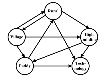
Figure 1: Directed network composed of five labels.

Usually, there are two kinds of relationships among labels, i.e., positive relationship and negative relationship. Positive relationship refers to the co-occurrence or co-disappearance of labels, as shown in Fig. 2(a), when ${\rm Rural}$ appears in an image, ${\rm Village}$ or ${\rm Paddy}$ is also likely to appear; while negative relationship refers to the mutually exclusive relations of labels, as shown in Fig. 2(b), when ${\rm Rural}$ appears, ${\rm High\ building}$ or ${\rm Technology}$ is unlikely to appear. Both positive and negative relationships are useful for modeling the label correlations.

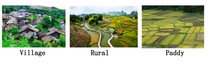
(a) Positive relationship between Rural-Village or Rural-Paddy

(b) Negative relationship between Rural-High building or Rural-Technology

Figure 2: Relationships among labels.

Classifier chain (CC) is a PTM that tries to make use of the label correlations [44]. Similar to BR, CC constructs $|\mathbb{L}|$ binary classifiers and each classifier is responsible for predicting the relevance of one label. However, the classifiers are trained sequentially by following a pre-defined label order, and the input feature vector for one label is extended by the labels ordered before it. The key issue in CC approach is to find the optimal label order. If the predecessors of a label are highly correlated to it, then the extended features can help improve the performance of the corresponding classifier, otherwise not. Original CC approach determines the label order randomly, which has a risk of low performance and low robustness. Later, ensemble CC (ECC) was proposed [45]. It trains multiple CCs based on different random orders, and gets the final prediction by collective voting. ECC can reduce the risk of low performance, but the time complexity is high. Another scheme called double-Monte Carlo CC (M2CC) was proposed [43], which models the dependencies of labels based on their co-occurrence. It finds the possible chain-sequences during training stage and determines the best chain by efficient inference through Monte Carlo optimization. Furthermore, group sensitive CC (GCC) was proposed [14] by considering local and positive label correlations. To assume that similar instances tend to have similar labels, GCC clusters the instances into groups. It builds a CC for each group and predicts an unseen instance by the CC trained on its nearest group. Moreover, enhanced CC with $k$-means clustering algorithm ($k$m-CC) was proposed [67]. By employing $k$-means algorithm several times, correlations among labels are discovered and the order of classifiers is determined. It is noteworthy that the above-introduced methods can help improve the performance of CC approach, but the time complexity is usually high. Besides, most of them analyze label correlations based on co-occurrence, whereas the mutually exclusive relations are neglected. According to these disadvantage, a comprehensive model is desired for label correlation analysis

Bayesian network (BN), known as a directed acyclic graph (DAG), is a probabilistic graphical model that learns the properties of a set of random variables and their conditional probability distributions [41]. BN has a wide range of applications such as data mining [40], fault detection [1], safety analysis [68], agricultural research [10], bioinformatics [49, 37], and so on. In general, nodes in BN represent random variables, and edges connecting two nodes represent the relations between variables. If there is no edge connecting two nodes, then the two random variables are independent of each other. Conversely, if two nodes are connected by an edge, then the parent node (i.e., start-point of the edge) and the child node (i.e., end-point of the edge) are causally or non-conditionally dependent, which will generate a conditional probability value. By imposing a BN constraint on the random order, an improved CC approach with tree-based structure was proposed [47]. Furthermore, BN-augmented naive Bayes classifiers are used as the base models for CC approach [54]. However, to the best of our knowledge, using BN model for comprehensive label correlation analysis has not been investigated yet, which will be the main focus of this paper. By further introducing a fast label ordering method, a new BN-based CC approach (BNCC) is proposed. The contributions of this paper are listed as follows:

• Conditional entropy is used to model the dependency degree of a label on other labels, which makes use of both positive relationship and negative relationship. A fully connected directed cyclic graph (DCG) is built up as the initial structure, where nodes represent labels and weights of edges indicate the dependency degrees among connected labels.

• An algorithm is proposed to refine a DCG into a DAG by breaking cycles iteratively, which guarantees to generate effective BN structure. We also propose to use topological sorting on the nodes of a DAG, in order to get efficacious label order from a BN structure.

• A new scoring function is proposed to evaluate the quality of BN, which includes the dependency degree calculated by conditional entropy and a complexity penalization term. Since learning the optimal BN is inference intractable, a heuristic algorithm is proposed to get approximate solutions based on the scoring function.

• We conduct extensive experimental comparisons between the proposed method and several state-of-the-art MLL approaches. Empirical studies show that the proposed method can generate effective CC model with a relatively low time complexity in both training and testing.

The remainder of this paper is organized as follows. In section 2, we introduce some background knowledge. In section 3, we present our proposed method. In section 4, extensive experimental comparisons are conducted to show the advantages of the proposed method. Finally, conclusions are given in section 5.

2 Background Knowledge

In this section, we will present some background knowledge on CC approach, label correlation, and BN model.

2.1 CC Approach

Suppose that $\mathcal{X}=\mathbf{R}^{d}$ is a $d$-dimensional instance space, $\mathbb{L}=\{l_{1},\ldots,l_{M}\}$ is a label set, and $\mathcal{Y}=\{0,1\}^{M}$ is a decision space with regard to $\mathbb{L}$. We denote by $\mathbb{D}=\{(\mathbf{x}_{i},\mathbf{y}_{i})\}_{i=1}^{N}$ as the training set with $N$ instances, where $\mathbf{x}_{i}=[x_{i1},x_{i2},\ldots,x_{id}]\in\mathcal{X}$ is the feature vector for the $i$-th instance and $\mathbf{y}_{i}=[y_{i1},y_{i2},\ldots,y_{iM}]\in\mathcal{Y}$ is the label vector of $\mathbf{x}_{i}$. We have $y_{ij}=1$ if $\mathbf{x}_{i}$ has the $j$-th label and $y_{ij}=0$ otherwise, where $j=1,2,\ldots,M$. MLL aims to train a function $h:\mathcal{X}\rightarrow\mathcal{Y}$ from $\mathbb{D}$, such that $h$ can predict the label vector of unseen instance $\hat{\mathbf{x}}$, i.e., $\hat{\mathbf{y}}=h(\hat{\mathbf{x}})$.

CC approach decomposes the $M$-label problem into a chain of $M$ binary problems. One classifier in the chain deals with a binary problem regarding a label in $\mathbb{L}$. In the training phase, the binary classifiers are constructed following a pre-defined order, where the input feature vector for the current classifier is extended by the previous labels. In specific, CC approach firstly generates a new order of the labels by a permutation function $\tau$, i.e.,

$$\tau:\{1,\ldots,M\}\rightarrow\{1,\ldots,M\}.$$

The training set for $l_{\tau(1)}$ is $\mathbb{D}_{1}=\{(\mathbf{x}_{i},{y}_{i\tau(1)})\}_{i=1}^{N}$, and the first classifier is constructed as $h_{1}:\mathbf{R}^{d}\rightarrow\{0,1\}$. Then, the training set for $l_{\tau(2)}$ is extended as $\mathbb{D}_{2}=\{([\mathbf{x}_{i},{y}_{i\tau(1)}],{y}_{i\tau(2)})\}_{i=1}^{N}$, and the second classifier is constructed as $h_{2}:\mathbf{R}^{d+1}\rightarrow\{0,1\}$. Following this rule, the general form of the training set for $l_{\tau(j)}$ is

$$\mathbb{D}_{j}=\{([\mathbf{x}_{i},{\rm\bf Pre}_{i\tau(j)}],{y}_{i\tau(j)})\}_{i=1}^{N},$$

where ${\rm\bf Pre}_{i\tau(j)}=[{y}_{i\tau(1)},{y}_{i\tau(2)},\ldots,{y}_{i\tau(j-1)}]$, and ${\rm\bf Pre}_{i\tau(1)}=\emptyset$. As a result, the $j$-th classifier is constructed as

$$h_{j}:\mathbf{R}^{d+j-1}\rightarrow\{0,1\},$$

where $j=1,2,\ldots,M$.

In the testing phase, given an unseen instance $\hat{\mathbf{x}}$, the decision for $\l_{\tau(1)}$ is predicted as $\hat{y}_{\tau(1)}=h_{1}(\hat{\mathbf{x}})$. The decision for $l_{\tau(2)}$ is predicted as $\hat{y}_{\tau(2)}=h_{2}([\hat{\mathbf{x}},h_{1}(\hat{\mathbf{x}})])$. Following this rule, the decision for $l_{\tau(j)}$ is predicted as

$$\hat{y}_{\tau(j)}=h_{j}([\hat{\mathbf{x}},\hat{{\rm\bf Pre}}_{\tau(j)}]),$$

where $\hat{{\rm\bf Pre}}_{\tau(j)}=[\hat{{\rm\bf Pre}}_{\tau(j-1)},h_{j-1}([\hat{\mathbf{x}},\hat{{\rm\bf Pre}}_{\tau(j-1)}])]$, $\hat{{\rm\bf Pre}}_{\tau(1)}=\emptyset$, and $j=1$, $2$, $\ldots$, $M$.

Table 1 shows the extended feature vectors of a training instance $(\mathbf{x},\mathbf{y})=([0.8,2.5,0.6,1.3,4.2],[1,0,1,0,0,1])$ in a six-label problem. Suppose that the label order is determined as $\tau:[1,2,3,4,5,6]\rightarrow[2,4,1,6,5,3]$, then six classifiers are trained by strictly following the order $\tau$, where $h_{j}$ is responsible for predicting the relevance of $l_{\tau(j)}$, $j=1,2,\ldots,6$.

In CC approach, if a label is strongly correlated to its predecessors, the extended feature dimensions can help improve the performance of the corresponding classifier, otherwise, the result will not be influenced or even degraded. That is, the performance highly relies on the label order $\tau$. How to get the optimal $\tau$ is still an ongoing research topic.

Table 1: Extended Feature Vectors for CC Approach

$j$	$l_{\tau(j)}$	Feature vector $[\mathbf{x},{\rm\bf Pre}_{\tau(j)}]$ for training $h_{j}$	$y_{\tau(i)}$
$1$	$l_{2}$	$[0.8,2.5,0.6,1.3,4.2]$	0
$2$	$l_{4}$	$[0.8,2.5,0.6,1.3,4.2,0]$	0
$3$	$l_{1}$	$[0.8,2.5,0.6,1.3,4.2,0,0]$	1
$4$	$l_{6}$	$[0.8,2.5,0.6,1.3,4.2,0,0,1]$	1
$5$	$l_{5}$	$[0.8,2.5,0.6,1.3,4.2,0,0,1,1]$	0
$6$	$l_{3}$	$[0.8,2.5,0.6,1.3,4.2,0,0,1,1,0]$	1

2.2 Correlations Among Labels

Given a $M$-label problem with $\mathbb{L}=\{l_{1},l_{2},\dots,l_{M}\}$, we use $l_{j}$ to denote the name of the $j$-th label and $y_{j}\in\{0,1\}$ to denote a specific value that $l_{j}$ can take. Considering any pair of distinct labels $l_{j},l_{k}\in\mathbb{L}$ ($l_{j}\neq l_{k}$), it is known that $p(l_{j}=y_{j},l_{k}=y_{k})$ is the joint probability, $p(l_{j}=y_{j})$ and $p(l_{k}=y_{k})$ are the marginal probabilities, $p(l_{j}=y_{j}|l_{k}=y_{k})$ and $p(l_{k}=y_{k}|l_{j}=y_{j})$ are the conditional probabilities. We denote $p(l_{j}=y_{j},l_{k}=y_{k})$, $p(l_{j}=y_{j})$, $p(l_{k}=y_{k})$, $p(l_{j}=y_{j}|l_{k}=y_{k})$ and $p(l_{k}=y_{k}|l_{j}=y_{j})$ as $p(y_{j},y_{k})$, $p_{l_{j}}(y_{j})$, $p_{l_{k}}(y_{k})$, $p_{l_{j}}(y_{j}|y_{k})$ and $p_{l_{k}}(y_{k}|y_{j})$ for short. Then, the following remarks hold.

1. $p_{l_{j}}(y_{j})=\sum\nolimits_{y_{k}\in\{0,1\}}p(y_{j},y_{k})$ and $p_{l_{k}}(y_{k})=\sum\nolimits_{y_{j}\in\{0,1\}}p(y_{j},y_{k})$.

2. $\sum\nolimits_{y_{j}\in\{0,1\}}p_{l_{j}}(y_{j})=\sum\nolimits_{y_{k}\in\{0,1\}}p_{l_{k}}(y_{k})=1$.

3. $p(y_{j},y_{k})=p_{l_{j}}(y_{j})\times p_{l_{k}}(y_{k}|y_{j})=p_{l_{k}}(y_{k})\times p_{l_{j}}(y_{j}|y_{k})$.

Based on these remarks, the following definition is given.

Definition 1.

(Label Independence) Given a pair of labels $(l_{j},l_{k})$ and their probability distributions, $l_{j}$ and $l_{k}$ are considered as independent if and only if they satisfy

$$p(y_{j},y_{k})=p_{l_{j}}(y_{j})\times p_{l_{k}}(y_{k})$$ (1)

for any $y_{j},y_{k}\in\{0,1\}$.

From Definition 1 and Remark 3, it is easy to know that if $l_{j}$ and $l_{k}$ are independent, the marginal probability equals to conditional probability, i.e., $p_{l_{j}}(y_{j})=p_{l_{j}}(y_{j}|y_{k})$ and $p_{l_{k}}(y_{k})=p_{l_{k}}(y_{k}|y_{j})$. Let us consider a specific example in Table 2, where the probabilities are calculated from an artificial data set. We can obtain $p(0,0)=0.4$ and $p_{l_{1}}(0)\times p_{l_{2}}(0)=0.4\times 0.7=0.28$, thus we have $p(0,0)\neq p_{l_{1}}(0)\times p_{l_{2}}(0)$. This inequality also holds for $p(0,1)$, $p(1,0)$, and $p(1,1)$. In this case, $l_{1}$ and $l_{2}$ are not independent, and this phenomenon exits in almost all multi-label data sets.

Table 2: An Example for Label Probabilities

$p(y_{1},y_{2})$	$y_{2}=0$	$y_{2}=1$	$p_{l_{1}}(y_{1})$
$y_{1}=0$	$0.4$	$0.0$	$0.4$
$y_{1}=1$	$0.3$	$0.3$	$0.6$
$p_{l_{2}}(y_{2})$	$0.7$	$0.3$	1

In classical correlation analysis, we know that if two variables are independent, then they are linearly uncorrelated. Conversely, if two variables are not independent, linear correlation may exist between them. However, in MLL, traditional linear correlation coefficient may not be a good measure due to the binary value configuration for each label. Designing a meaningful correlation model is a key issue in this work.

Moreover, most existing works for label correlation analysis only consider the co-occurrence of two labels. In this paper, we define the co-occurrence and co-disappearance of two labels, i.e., $p(1,1)$ and $p(0,0)$, as positive relationships, and the mutually exclusive relations, i.e., $p(0,1)$ and $p(1,0)$, as negative relationships, which will be utilized together to improve CC approach.

2.3 BN Model

BN is a probabilistic graphical model that captures the dependency relations among a set of variables by a DAG. A BN is denoted by $\mathcal{B}=(\mathbb{G},\Theta)$, which consists of two components, i.e., $\mathbb{G}$ and $\Theta$. The first component $\mathbb{G}=(\mathbb{V},\mathbb{E})$ is a DAG, where $\mathbb{V}$ is a set of nodes and $\mathbb{E}$ is a set of directed edges connecting the nodes. Usually, each node represents a random variable and each edge represents a directed dependency relation between two variables. The second component $\Theta$ is a set of parameters that measures the network, which is described by a set of conditional probabilities.

In this paper, we discuss BN under MLL scenario, thus nodes represent labels and edges reflect label correlations. According to the classical chain rule, a unique joint probability distribution over $\mathbb{L}$ is given by

$$\centering\begin{split}p(y_{1},\dots,y_{M})=p(y_{1})p(y_{2}|y_{1})p(y_{3}|y_{1},y_{2})\\ \dots p(y_{M}|y_{1},y_{2},\ldots,y_{M-1}).\end{split}\@add@centering$$ (2)

Considering the conditional probabilities in Eq. (2), we have the following definition.

Definition 2.

(Conditional Independence) Let $p$ be a joint probability distribution over the labels in $\mathbb{L}$, and $\{l_{j},l_{k},l_{q}\}$ be a subset of $\mathbb{L}$. If $p(y_{j}|y_{k},y_{q})=p(y_{j}|y_{q})$ holds for all possible combinations of $y_{j},y_{k},y_{q}\in\{0,1\}$, then we say that $l_{j}$ and $l_{k}$ are conditionally independent given $l_{q}$.

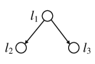
(a) Tail-to-Tail

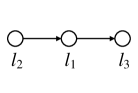
(b) Head-to-Tail

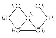
(c) BN Structure

Figure 3: Conditional independence relations in BN.

The conditional independence relation can be proved for the tail-to-tail case and head-to-tail case in BN. As show in Figures 3(a) and 3(b), $l_{2}$ and $l_{3}$ are conditionally independent given $l_{1}$. By applying this rule, the number of parameters in Eq. (2) can be largely reduced. For example, the joint probability distribution in Figure 3(c) can be simplified as

$$\centering\begin{split}p(y_{1},\dots,y_{7})=p(y_{1})p(y_{2}|y_{1})p(y_{3}|y_{2})\\ \cdots p(y_{7}|y_{4},y_{5},y_{6}).\end{split}\@add@centering$$ (3)

As a result, BN defines a unique joint probability distribution over $\mathbb{L}$, which can be generally expressed as

$$p(y_{1},y_{2},\dots,y_{M})=\prod_{j=1}^{M}\theta_{y_{j}|{\rm Pa}(y_{j})}=\prod_{j=1}^{M}p(y_{j}|{\rm Pa}(y_{j})),$$ (4)

where $\theta$ means a specification of $\Theta$, and ${\rm Pa}(y_{j})$ denotes the set of parents of $y_{j}$ in $\mathbb{G}$. BN can capture the complex correlations among multiple labels, thus, it is a promising technique to improve the performance of CC approach.

3 The Proposed BNCC Method

In this section, we will propose the BN model for label correlation analysis and the BNCC method for MLL.

3.1 Modeling Label Correlations

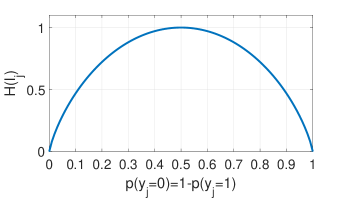
Figure 4: Uncertainty of a single label.

In order to model the correlations among multiple labels, we first give an analysis on the uncertainty of a single label.

Definition 3.

(Uncertainty of a Label) Given a single label $l_{j}\in\mathbb{L}$, the uncertainty of its decision is defined by classical entropy:

$$\mathcal{H}(l_{j})=-\sum_{y_{j}\in\{0,1\}}p(y_{j})\log p(y_{j}).$$ (5)

As shown in Figure 4, $\mathcal{H}(l_{j})$ will attain its maximum when $l_{j}$ can be assigned to the positive and negative decisions with an equal probability, and will attain its minimum when $l_{j}$ can only be assigned to the positive or negative decision. Having this classical definition, we further consider $l_{j}$ under the condition of another label $l_{k}$, and raise a question that when the decision of $l_{k}$ is given, what is the uncertainty of deciding $l_{j}$? In order to answer this question, the following definition is given.

Definition 4.

(Conditional Uncertainty of a Label Under Another Label) Given a pair of labels $l_{j},l_{k}\in\mathbb{L}$ ($l_{j}\neq l_{k}$), the uncertainty of $l_{j}$ under the condition of $l_{k}$, denoted as $\mathcal{H}(l_{j}|l_{k})$, is defined by conditional entropy:

$$\begin{array}[]{llll}\mathcal{H}(l_{j}|l_{k})\\ =\sum_{y_{k}\in\{0,1\}}p(y_{k})\mathcal{H}(l_{j}|y_{k})\\ =-\sum_{y_{k}\in\{0,1\}}p(y_{k})\sum_{y_{j}\in\{0,1\}}p(y_{j}|y_{k})\log p(y_{j}|y_{k})\\ =-\sum_{y_{k}\in\{0,1\}}\sum_{y_{j}\in\{0,1\}}p(y_{j},y_{k})\log p(y_{j}|y_{k})\\ =-\sum_{y_{k}\in\{0,1\}}\sum_{y_{j}\in\{0,1\}}p(y_{j},y_{k})\log\frac{p(y_{j},y_{k})}{p(y_{k})}\\ =\sum_{y_{k}\in\{0,1\}}\sum_{y_{j}\in\{0,1\}}p(y_{j},y_{k})\log\frac{p(y_{k})}{p(y_{j},y_{k})}\end{array}.$$ (6)

It is easy to prove that the conditional entropy $\mathcal{H}(l_{j}|l_{k})$ in Definition 4 has the following properties:

• $\mathcal{H}(l_{j}|l_{k})\in[0,1]$ reflects the amount of information that $l_{k}$ carries about $l_{j}$, i.e., the larger value of $\mathcal{H}(l_{j}|l_{k})$, the less information $l_{k}$ carries about $l_{j}$, and vice versa;

• $\mathcal{H}(l_{j}|l_{k})$ attains its minimum $0$ if and only if the value of $l_{j}$ can be completely predicted by the value of $l_{k}$;

• $\mathcal{H}(l_{j}|l_{k})$ attains its maximum $1$ when the value of $l_{k}$ has no help in deciding the value of $l_{j}$;

• $\mathcal{H}(l_{j}|l_{k})\neq\mathcal{H}(l_{k}|l_{j})$, which means that conditional entropy has the property of asymmetry, i.e., the uncertainty of deciding $l_{j}$ when given $l_{k}$ is different from the uncertainty of deciding $l_{k}$ when given $l_{j}$.

Having the above analyses, we know that $\mathcal{H}(l_{j}|l_{k})$ could be treated as the level of difficulty in deciding $l_{j}$ based on $l_{k}$, which also reflects the independence degree of $l_{j}$ on $l_{k}$.

Definition 5.

(Dependence Degree) Given a pair of labels $l_{j},l_{k}\in\mathbb{L}$ ($l_{j}\neq l_{k}$), the dependence degree of $l_{j}$ on $l_{k}$ (also called the influence degree of $l_{k}$ on $l_{j}$), denoted by $\mathcal{I}(l_{k}\rightarrow l_{j})$, is defined as:

$$\mathcal{I}(l_{k}\rightarrow l_{j})=1-\mathcal{H}(l_{j}|l_{k}).$$ (7)

Definition 5 provides a way to evaluate the informativeness of a directed edge in a graph, which can help construct an initial structure for BN. Furthermore, both positive relationships, i.e., $p(1,1)$ and $p(0,0)$, and negative relationships, i.e., $p(1,0)$ and $p(0,1)$, are included in Eq. (6). Thus, it has taken into account all the possible relations between two labels.

The conditional uncertainty of a label can be further extended by revising the condition from a single label $l_{k}$ to a label subset $\mathbb{L}^{*}\subset\mathbb{L}$. Then, the following definition is given.

Definition 6.

(Conditional Uncertainty of a Label Under a Label Set) Given a single label $l_{j}\in\mathbb{L}$ and a label subset $\mathbb{L}^{*}\subset\mathbb{L}$ where $l_{j}\notin\mathbb{L}^{*}$, the uncertainty of $l_{j}$ under the condition of $\mathbb{L}^{*}$, denoted by $\mathcal{H}(l_{j}|\mathbb{L}^{*})$, is defined as:

$$\begin{array}[]{llll}\mathcal{H}(l_{j}|\mathbb{L}^{*})\\ =\sum_{\mathcal{L}^{*}\in\{0,1\}^{\mathbb{L}^{*}}}p(\mathcal{L}^{*})\mathcal{H}(l_{j}|\mathcal{L}^{*})\\ =\sum_{\mathcal{L}^{*}\in\{0,1\}^{\mathbb{L}^{*}}}\sum_{y_{j}\in\{0,1\}}p(y_{j},\mathcal{L}^{*})\log\frac{p(y_{k})}{p(y_{j},\mathcal{L}^{*})}\end{array},$$ (8)

where $\mathcal{L}^{*}$ represents a possible value configuration for the labels in $\mathbb{L}^{*}$.

Similarly, the dependence degree of $l_{j}$ on $\mathbb{L}^{*}$ (also called the influence degree of $\mathbb{L}^{*}$ on $l_{j}$), denoted by $\mathcal{I}(\mathbb{L}^{*}\rightarrow l_{j})$, is defined as:

$$\mathcal{I}(\mathbb{L}^{*}\rightarrow l_{j})=1-\mathcal{H}(l_{j}|\mathbb{L}^{*}).$$ (9)

3.2 Designing Scoring Function for BN

Having the definitions mentioned above, a fully connected DCG can be build up by linking each pair of labels in two-way, denoted as $\mathbb{G}^{\circ}=(\mathbb{V},\mathbb{E}^{\circ})$. There will be two links between every pair of labels $l_{j}$ and $l_{k}$, i.e., $l_{j}\rightarrow l_{k}$ and $l_{k}\rightarrow l_{j}$. We know that $\mathcal{I}(l_{k}\rightarrow l_{j})$ is the weight of link $l_{k}\rightarrow l_{j}$, which represents the dependence degree of $l_{j}$ on $l_{k}$, and $\mathcal{I}(l_{j}\rightarrow l_{k})$ is the weight of link $l_{j}\rightarrow l_{k}$, which represents the dependence degree of $l_{k}$ on $l_{j}$. Thus, there will be $2\times\mathbf{C}_{M}^{2}$ edges with many directed cycles in $\mathbb{G}^{\circ}$, which is a complex structure to be optimized. The following two issues need to be resolved:

1. given a DCG, how to simplify it into an effective BN structure without cycles;

2. how to define a scoring function to evaluate a BN structure.

In order to handle the first issue, we refine a DCG into a DAG by breaking cycles iteratively. As we know, larger value of $\mathcal{I}(l_{k}\rightarrow l_{j})$ represents stronger dependence of $l_{j}$ on $l_{k}$. Thus, we iteratively break a cycle through removing the edge with the lowest dependence degree in the cycle, until a DAG is obtained. The detailed steps are described in Algorithm 1.

Input: Original DCG, denoted as $\mathbb{G}^{\circ}=(\mathbb{V},\mathbb{E}^{\circ})$;

     Dependence degree between any pair of labels, denoted as $\mathcal{I}$ .

Output: Refined DAG, i.e., $\mathbb{G}=(\mathbb{V},\mathbb{E})$.

1

2Let $\mathbb{G}=\mathbb{G}^{\circ}$;

3 while $\mathbb{G}$ has circles do

4       Find a circle in $\mathbb{G}$, denoted as $Cyc$;

5       Let $\mathbb{E}^{*}$ contain all the edges in $Cyc$, i.e., $\mathbb{E}^{*}=\{e|e\in Cyc\}$;

6       Find the edge in $\mathbb{E}^{*}$ with minimum dependence degree $e^{*}=\operatorname*{argmin}_{e\in\mathbb{E}^{*}}\mathcal{I}(e_{\rm start}\rightarrow e_{\rm end})$;

7       Delete $e^{*}$ from $\mathbb{G}$;

8

9return $\mathbb{G}$.

Algorithm 1 Refine a DCG into a DAG

As for the second issue, the most well-known scoring function for BN is the Bayesian information criterion (BIC), i.e.,

$$S_{\mathbb{D}}(\mathbb{G})=L_{\mathbb{D}}(\mathbb{G})-\frac{{\rm Dim}_{\mathbb{G}}}{2}\log N.$$ (10)

In Eq. (10), the first term is the log-likelihood of graph $\mathbb{G}$ with respect to the training set $\mathbb{D}$, which reflects the fitting degree between $\mathbb{G}$ and the data. In this paper, since the purpose is to model the correlations among multiple labels through BN, we re-define $L_{\mathbb{D}}(\mathbb{G})$ by using the dependence degree proposed in section 3.1. Finally, $L_{\mathbb{D}}(\mathbb{G})$ can be written as the sum of the scores for each label $l_{j}$, i.e.,

$$\begin{array}[]{llll}L_{\mathbb{D}}(\mathbb{G})\\ =N\sum\limits_{j=1}^{M}(\mathcal{I}(\mathbb{L}^{*}\rightarrow l_{j}))\\ =N\sum\limits_{j=1}^{M}(1-\mathcal{H}(l_{j}|{\rm Pa}(l_{j})))\\ =N(1-\sum\limits_{j=1}^{M}\sum\limits_{q=1}^{Q_{j}}p({\rm Pa}_{q}(l_{j}))\mathcal{H}(l_{j}|{\rm Pa}_{q}(l_{j})))\\ =N+N\sum\limits_{j=1}^{M}\sum\limits_{q=1}^{Q_{j}}\sum\limits_{y_{j}\in\{0,1\}}p(y_{j},{\rm Pa}_{q}(l_{j}))\log\frac{p(y_{j},{\rm Pa}_{q}(y_{j}))}{p({\rm Pa}_{q}(y_{j}))}\end{array},$$ (11)

where $Q_{j}$ represents the number of possible value configurations for ${\rm Pa}(l_{j})$, and ${\rm Pa}_{q}(l_{j})$ represents the $q$-th configuration. Furthermore, given data set $\mathbb{D}$, the probability can be calculated by frequency, thus we have

$$\begin{array}[]{llll}L_{\mathbb{D}}(\mathbb{G})\\ =N+N\sum\limits_{j=1}^{M}\sum\limits_{q=1}^{Q_{j}}\sum\limits_{y_{j}\in\{0,1\}}\frac{N_{jq}^{(y_{j})}}{N}\log\frac{N_{jq}^{(y_{j})}}{N_{jq}}\\ =N+\sum\limits_{j=1}^{M}\sum\limits_{q=1}^{Q_{j}}\sum\limits_{y_{j}\in\{0,1\}}N_{jq}^{(y_{j})}\log\frac{N_{jq}^{(y_{j})}}{N_{jq}}\end{array},$$ (12)

where $N_{jq}$ indicates the number of instances in $\mathbb{D}$ with the $q$-th configuration for ${\rm Pa}(l_{j})$, and $N_{jq}^{(y_{j})}$ indicates the number of instances in $\mathbb{D}$ with $l_{j}=y_{j}$ given the $q$-th configuration for ${\rm Pa}(l_{j})$.

In Eq. (10), the second term is a complexity penalization factor, which prevents over-fitting between $\mathbb{G}$ and the training data. It can be denoted by the number of independent parameters in the structure, i.e., ${\rm Dim}_{\mathbb{G}}=\sum_{j=1}^{M}Q_{j}$. Finally, the scoring function becomes

$$\begin{array}[]{llll}S_{\mathbb{D}}(\mathbb{G})\\ =N+\sum\limits_{j=1}^{M}\sum\limits_{q=1}^{Q_{j}}\sum\limits_{y_{j}\in\{0,1\}}N_{jq}^{(y_{j})}\log\frac{N_{jq}^{(y_{j})}}{N_{jq}}-\sum\limits_{j=1}^{M}\frac{Q_{j}}{2}\log N.\end{array}$$ (13)

3.3 Learning the Optimal BN Structure

In order to learn the optimal BN based on a given data set, all possible structures can be considered as a domain, and the scoring function is used to measure the quality of a structure in the domain. Finding the best BN structure is equivalent to find the maximum value of the scoring function. However, the number of candidate structures is huge, it is impossible to traverse all of them. Since the scoring function can be decomposed with regard to different labels $l_{j}$ ($j=1,\ldots,M$), we can find the optimal parent set for each individual label separately. In this case, an initial label order should be determined, such that the labels can be optimized one-by-one. Topological sorting [16] gives a good solution for ordering the nodes in a DAG, which is presented in Algorithm 2.

Input: DAG $\mathbb{G}=(\mathbb{V},\mathbb{E})$, where $\mathbb{V}=\{l_{1},l_{2},\ldots,l_{M}\}$.

Output: Label order $\alpha:{l_{\alpha(1)},l_{\alpha(2)},\ldots,l_{\alpha(M)}}$.

1

2Let $\mathbb{V}^{*}=\mathbb{V}$;

3 for each node $l$ in $\mathbb{V}^{*}$ do

4       Calculate the in-degree of $l$ in $\mathbb{G}$, denoted as $\mathfrak{in}(l)$;

5      

6for $j=1$ to $M$ do

7       Select a node from $\mathbb{V}^{*}$ with $\mathfrak{in}(l)=0$, denoted as $l^{*}$;

8       Let $l_{\tau(j)}=l^{*}$, $\mathbb{V}^{*}=\mathbb{V}^{*}\setminus l^{*}$;

9       for each node $l$ pointed to by $l^{*}$ do

10             Let $\mathfrak{in}(l)=\mathfrak{in}(l)-1$;

11            

12      

13

14return Label order $\alpha:{l_{\alpha(1)},l_{\alpha(2)},\dots,l_{\alpha(M)}}$.

Algorithm 2 Topological Sorting for Nodes in a DAG

Having the label order derived from Algorithm 2, the optimal parent set can be discovered for each label separately. In [9] and [2], two algorithms called K2 and K3 were developed for this purpose, they begin with an empty parent set for each label and add new members to the set based on a greedy strategy. In this paper, we propose a similar strategy by applying the newly proposed scoring function.

Due to the decomposition characteristic of the scoring function, the optimal graph can be constructed by building and merging the optimal sub-graphs for individual labels. Let $\mathbb{G}_{l|{\rm Pa}(l)}$ be the sub-graph that is only composed of $l$ and ${\rm Pa}(l)$, and assume that an initial label order $\alpha:$ $l_{\alpha(1)}$, $l_{\alpha(2)}$, $\dots$, $l_{\alpha(M)}$ is produced by Algorithm 2. Then, the details for optimal parent set determination are described in Algorithm 3. Several key points are highlighted as follows.

• For $l_{\alpha(j)}$, $j=1,2,\ldots,M$, the parent set ${\rm Pa}(l_{\alpha(j)})$ is initialized as $\emptyset$ and the candidate set ${\rm Pred}_{j}$ is initialized as $\mathbb{L}\setminus l_{\alpha(j)}$. The candidate in ${\rm Pred}_{j}$ that can maximize the gain of score for $\mathbb{G}_{l_{\alpha(j)}|{\rm Pa}(l_{\alpha(j)})}$ will be added to ${\rm Pa}(l_{\alpha(j)})$ iteratively.

• Structural anomalies may appear in the learned graph, i.e., one node may have too many child nodes, causing the structure to be over-wide and obstructing the graph from including more meaningful edges. As shown in Figure 5, structure 2 is more ideal than structure 1 since structure 2 captures more diverse relationships. In this case, we control the number of child nodes by setting a threshold.

• It is known from literature that in the optimal BN, each label has at most $\log N$ parents. Thus, we terminate the selection process for $l_{\alpha(j)}$ when $|{\rm Pa}(l_{\alpha(j)})|>\log N$.

Input: Training set $\mathbb{D}=\{(\mathbf{x}_{i},\mathbf{y}_{i})\}_{i=1}^{N}$ and label set $\mathbb{L}=\{l_{1},l_{2},\ldots,l_{M}\}$;

     Initial label order $\alpha:{l_{\alpha(1)},l_{\alpha(2)},\ldots,l_{\alpha(M)}}$;

     Threshold $n$ for maximum number of child nodes.

Output: Graph $\mathbb{G}_{\rm new}^{\circ}$ with optimized parent label sets.

1

2Let $\mathbb{G}_{\rm new}^{\circ}$ be an empty graph;

3 for $j=1$ to $M$ do

4       Let ${\rm Pred}_{j}=\mathbb{L}\setminus l_{\alpha(j)}$;

5       Let ${\rm Pa}(l_{\alpha(j)})=\emptyset$;

6       for each $l\in{\rm Pred}_{j}$ do

7             if $l$ already has $n$ child nodes then

8                   ${\rm Pred}_{j}={\rm Pred}_{j}\setminus l$;

9                  

10            

11      Let $S_{\rm opt}=-\infty$;

12       while $|{\rm Pa}(l_{\alpha(j)})|\leq\log N$ and ${\rm Pred}_{j}\neq\emptyset$ do

13             Let $l^{*}=\operatorname*{argmax}_{l\in{\rm Pred}_{j}}S_{\mathbb{D}}(\mathbb{G}_{l_{\alpha(j)}|{\rm Pa}(l_{\alpha(j)})\bigcup l})$;

14             Let $S_{\rm new}=S_{\mathbb{D}}(\mathbb{G}_{l_{\alpha(j)}|{\rm Pa}(l_{\alpha(j)})\bigcup l^{*}})$;

15             if $S_{\rm new}>S_{\rm opt}$ then

16                   ${\rm Pa}(l_{\alpha(j)})={\rm Pa}(l_{\alpha(j)})\bigcup{{l^{*}}}$;

17                   ${\rm Pred}_{j}={\rm Pred}_{j}\setminus l^{*}$;

18                   $S_{\rm opt}=S_{\rm new}$;

19            else

20                   break;

21            

22      Update $\mathbb{G}_{\rm new}^{\circ}$ by merging $\mathbb{G}_{l_{\alpha(j)}|{\rm Pa}(l_{\alpha(j)})}$ into $\mathbb{G}_{\rm new}^{\circ}$;

23

return $\mathbb{G}_{\rm new}^{\circ}$.

Algorithm 3 Learning the Optimal Parent Set For Each Node

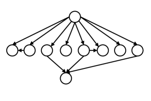
(a) Structure 1

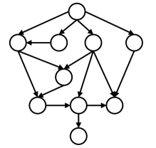
(b) Structure 2

Figure 5: Two BN structures for a ten-label problem.

It is noteworthy that the graph produced by Algorithm 3 may have cycles. Since the value of dependence degree is non-negative, and the larger the dependence degree of a label on its parents, the larger the score will be, i.e.,

$$\mathcal{I}(l_{k}\rightarrow l_{j})>\mathcal{I}(l_{q}\rightarrow l_{j})\Rightarrow S(\mathbb{G}_{l_{j}|l_{k}})>S(\mathbb{G}_{l_{j}|l_{q}}),$$ (14)

in this case, Algorithm 1 can be used again to refine the newly constructed DCG into an effective BN, and the final label order is obtained by applying Algorithm 2 on the BN.

3.4 Constructing CC Model

In this section, we summarize the process of building the CC model by learning the optimal BN. First, the dependence degree between any pair of labels is computed based on Definition 5, and a fully connected DCG $\mathbb{G}^{\circ}$ is constructed. Then, by breaking cycles in $\mathbb{G}^{\circ}$, an initial DAG $\mathbb{G}$ is produced and an initial label order is obtained by applying topological sorting on the nodes of $\mathbb{G}$. The optimal parent set for each label is learned following the initial order, and the learned sub-graphs for different labels are merged to be a new DCG $\mathbb{G}^{\circ}_{\rm new}$. Afterwards, the same process for breaking cycles is performed on $\mathbb{G}^{\circ}_{\rm new}$, and a new DAG $\mathbb{G}_{\rm new}$ is produced. The final label order is obtained by applying topological sorting on the nodes of $\mathbb{G}_{\rm new}$. The entire procedure for building the CC model is summarized in Algorithm 4.

Input: Training set $\mathbb{D}=\{(\mathbf{x}_{i},\mathbf{y}_{i})\}_{i=1}^{N}$ and label set $\mathbb{L}=\{l_{1},l_{2},\ldots,l_{M}\}$;

     Threshold $n$ for maximum number of child nodes.

Output: CC model $h_{1},h_{2},\ldots,h_{M}$.

1

2Calculate the dependence degree in two-way between any pair of labels based on Eq. (7), denoted as $\mathcal{I}$;

3 Build up a fully connected DCG with all labels, i.e., $\mathbb{G}^{\circ}$;

4 Call Algorithm 1 on $\mathbb{G}^{\circ}$ and $\mathcal{I}$ to get initial DAG $\mathbb{G}$;

5 Call Algorithm 2 on $\mathbb{G}$ to get the initial label order $\alpha:\ l_{\alpha(1)},l_{\alpha(2)},\ldots,l_{\alpha(M)}$;

6 Call Algorithm 3 on $\mathbb{D}$, $\alpha$ and $n$ to learn the new graph $\mathbb{G}^{\circ}_{\rm new}$ with optimized parent label set for each label;

7 Call Algorithm 1 on $\mathbb{G}^{\circ}_{\rm new}$ and $\mathcal{I}$ to get optimized DAG $\mathbb{G}_{\rm new}$;

8 Call Algorithm 2 on $\mathbb{G}_{\rm new}$ to get the final label order $\tau:\ l_{\tau(1)},l_{\tau(2)},\ldots,l_{\tau(M)}$;

9 Train the CC model $h_{1},h_{2},\ldots,h_{M}$ based on $\mathbb{D}$ and $\tau$;

10

11return CC model $h_{1},h_{2},\ldots,h_{M}$.

12

Algorithm 4 Constructing the BN-based CC Model

3.5 Complexity Analysis

It is easy to analyze that in Algorithm 1, breaking a cycle $Cyc$ has the linear complexity of $O(|Cyc|)$, where $|Cyc|$ is the number of edges in $Cyc$, and in Algorithm 2, the topological sorting on $M$ nodes has the maximum complexity of $O(M^{2})$. As for Algorithm 3, the optimal parent set determination process is performed regarding each label separately. For each label, the main time cost focuses on the while loop, i.e., steps 11$\sim$21. It is noteworthy that computing the scoring function, i.e., Equation (13), has the complexity of $O(MQ+M)$, where $M$ is the number of labels and $Q$ is the number of possible value configurations for the parents of a label. Let $u=MQ+M$ be a unit time cost, thus, during each while loop, computing the scoring function for all candidate parent nodes of $l_{\alpha(j)}$ has the complexity of $O(|{\rm Pred}_{j}|u)$, and selecting the best candidate has the complexity of $O(|{\rm Pred}_{j}|)$, where ${\rm Pred}_{j}$ contains all the remained candidates in the current iteration. The initial size of ${\rm Pred}_{j}$ is $M-1$ and it is reduced by one during each iteration. Since there are $\log N$ iterations at most, the while loop for each label has the maximum complexity of $O(Mu+(M-1)u+\ldots+(M-\log N+1)u)$.

4 Empirical Studies

In this section, we conduct extensive experiments to show the effectiveness and efficiency of the proposed method.

4.1 Methods and Data Sets for Performance Comparison

Five state-of-the-art MLL methods, as well as the proposed approach, are listed in this section for performance comparison.

Binary Relevance (BR)

BR is a baseline method that decomposes the multi-label problem into multiple independent binary problems and each binary problem corresponds to a single label [50].

Calibrated Label Ranking (CLR)

CLR transforms the multi-label problem into a label ranking problem by building a binary classifier for each pair of labels [11].

Classifier Chain (CC)

Traditional CC approach transforms the multi-label problem into a chain of binary problems based on a randomly generated label order [44].

Group sensitive Classifier Chain (GCC)

The basic idea of GCC is to cluster the training instances into $m$ different groups and learn the label correlation locally for each group to build a classifier chain [14]. The best parameter reported in the literature $m=5$ is adopted.

Ensemble Classifier Chains (ECC)

This method trains multiple CCs based on different random orders, and gets the final prediction by collective voting [45]. We set the number of CCs as 10 for the smaller data sets and set the number of CCs as 5 for the larger data sets.

Bayesian Network based Classifier Chain (BNCC)

The proposed approach is realized.

Eighteen data sets are selected for performance comparison. These data sets are collected from multiple sources including Mulan, Lamda, and Yahoo, which cover a wide range of application domains such as image recognition, music retrieval, text classification, and bio-informatics, etc. The details of the selected data sets are listed in Table 3.

Table 3: Data Sets for Performance Comparison

Data Sets	Domain	# Training	# Testing	# Attributes	# Labels	Card	AvgIR
Bibtex	Text	4,880	2,515	1,836	159	2.402	12.498
CHD49	Medicine	555	—	49	6	2.580	5.766
Emotions	Music	391	202	72	6	1.869	1.478
Enron	Text	1,123	579	1,001	53	3.378	73.953
EukaryoteGo	Biology	4,658	3,108	12,689	22	1.146	45.012
Flags	Image	129	65	19	7	3.392	2.255
Genbase	Biology	463	199	1,186	27	1.252	37.315
GramNegative	Biology	836	556	1,717	8	1.046	18.448
GramPositive	Biology	311	208	912	4	1.008	3.861
HumanGoB3106	Biology	3,106	—	9,844	14	1.185	15.289
HumanPseACC3106	Biology	1,862	—	440	14	1.185	15.289
Mediamill	Video	30,993	12,914	120	101	4.376	256.405
Medical	Text	333	645	1,449	45	1.245	89.501
PlantGoB978	Biology	588	390	3,091	12	1.079	6.690
Scene	Image	1,211	1,196	294	6	1.074	1.254
VirusGo	Biology	124	83	749	6	1.217	4.041
WaterQuality	Chemistry	1,060	—	16	14	5.073	1.767
Yeast	Biology	1,500	917	103	14	4.237	7.197

Note: Card represents label cardinality, i.e., the average number of positive labels associated with the samples; and AvgIR measures the average degree of imbalance of all labels, the greater avgIR, the greater the imbalance of the data set.

4.2 Evaluation Metrics

As observed from the last two columns of Table 3, multi-label data sets are usually imbalanced, i.e., the number of negative instances is much larger than the number of positive instances for each label. Usually, the purpose of MLL is to correctly identify the positive labels for unseen instances, thus, traditional measures like testing accuracy might be ineffective. In this paper, we utilize four metrics as follows.

4.2.1 Hamming Loss (${\rm HammingLoss}$)

${\rm HammingLoss}$ is an instance-based metric that evaluates how many times the instance-label pairs are misclassified, i.e.,

$${\rm HammingLoss}=\frac{1}{N}\sum_{i=1}^{N}\frac{1}{M}\sum_{j=1}^{M}\llbracket\mathbf{y}_{ij}\neq\hat{\mathbf{y}}_{ij}\rrbracket,$$ (15)

where $\llbracket\cdot\rrbracket$ returns 1 or 0 if the internal condition holds or not, $M$ is the number of labels, $N$ is the number of instances, $\mathbf{y}_{i}$ and $\hat{\mathbf{y}}_{i}$ are the ground-truth label vector and the predicted label vector for the $i$-th instance. ${\rm HammingLoss}$ treats the positive and negative labels as equally important. As mentioned above, due to the imbalance nature, it is highly biased by the results on the negative labels, thus is not a good measure for MLL.

4.2.2 Instance-based F-score (${\rm Fscore}$)

${\rm Fscore}$ is also an instance-based metric that computes a harmonic mean between precision and recall for each instance, i.e.,

$${\rm Fscore}=\frac{1}{N}\sum_{i=1}^{N}\frac{2{\rm Precision}_{i}\cdot{\rm Recall}_{i}}{{\rm Precision}_{i}+{\rm Recall}_{i}},$$ (16)

where ${\rm Precision}_{i}=$ ${\sum_{j=1}^{M}\llbracket\mathbf{y}_{ij}=1\&\&\hat{\mathbf{y}}_{ij}=1\rrbracket}/{\sum_{j=1}^{M}\llbracket\mathbf{y}_{ij}=1\rrbracket}$ and ${\rm Recall}_{i}=$ ${\sum_{j=1}^{M}\llbracket\mathbf{y}_{ij}=1\&\&\hat{\mathbf{y}}_{ij}=1\rrbracket}/{\sum_{j=1}^{M}\llbracket\hat{\mathbf{y}}_{ij}=1\rrbracket}$ are respectively the ratios of correctly predicted positive labels in the real positive set and in the set that has been predicted as positive for the $i$-th instance. Since this metric focuses on the correctly predicted positive labels for each instance, it is much more rational than ${\rm HammingLoss}$.

4.2.3 Label-based Macro F-score (${\rm MacF}$)

${\rm MacF}$ is a label-based metric that evaluates the macro average of precision and recall regarding different labels, i.e.,

$${\rm MacF}=\frac{1}{M}\sum_{j=1}^{M}\frac{2{\rm TP}_{j}}{2{\rm TP}_{j}+{\rm FP}_{j}+{\rm FN}_{j}},$$ (17)

where ${\rm TP}_{j}$, ${\rm FP}_{j}$, and ${\rm FN}_{j}$ are the numbers of true positives, false positives, and false negatives regarding the $j$-th label. It focuses on the correct positive predictions regarding each label, thus it is a rational measure for MLL.

4.2.4 Label-based Micro F-score (${\rm MicF}$)

${\rm MicF}$ is also a label-based metric, which is a revised version of ${\rm MacF}$, i.e.,

$${\rm MicF}=\frac{2\sum_{j=1}^{M}{\rm TP}_{j}}{2\sum_{j=1}^{M}{\rm TP}_{j}+\sum_{j=1}^{M}{\rm FP}_{j}+\sum_{j=1}^{M}{\rm FN}_{j}},$$ (18)

where ${\rm TP}_{j}$, ${\rm FP}_{j}$, and ${\rm FN}_{j}$ are same as in Eq. (17). ${\rm MicF}$ also focuses on the correct positive predictions, thus it is a rational measure for MLL.

Obviously, smaller value of ${\rm HammingLoss}$ and larger values of the three F-scores represent better performance of the model.

4.3 Experimental Setup

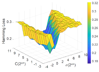
(a) ${\rm HammingLoss}$

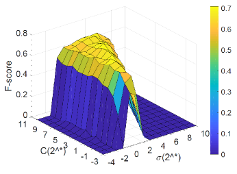
(b) ${\rm Fscore}$

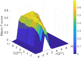
(c) ${\rm MacF}$

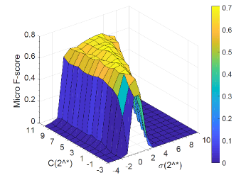
(d) ${\rm MicF}$

Figure 6: Sensitivity of SVM parameters regarding different metrics in BNCC on Emotions.

The base classifiers in all the compared methods are binary, thus support vector machine (SVM) [53, 57, 56] is used consistently, since it has been verified to be ideal binary model in many applications. Furthermore, non-linear SVM is realized by applying RBF kernel $\mathcal{K}(\mathbf{x},\mathbf{x}_{i})=\exp(-{\frac{||\mathbf{x}-\mathbf{x}_{i}||^{2}}{2\sigma^{2}}})$.

Since the performance of SVM is largely influenced by the model parameters, i.e., slack variable $C$ and kernel parameter $\sigma$, we first make an investigation on a small data set Emotions. We investigate the influences of $C$ and $\sigma$ on the performance of BNCC by tuning $C$ from [$2^{-3},2^{-2},\dots,2^{9},2^{10}$] and $\sigma$ from [$2^{-3},2^{-2},\dots,2^{8},2^{9}$], where the result is demonstrated in Figure 6. It can be observed that the four metrics are very sensitive to $\sigma$ while are relatively stable regarding $C$, and this observation can also be found for the other methods. Usually, a larger value of $C$ can help improve the performance but will increase the execution time. Thus, in order to reduce validation time, we fix $C=100$ and tune parameter $\sigma$ for each data set. We conduct 10-fold cross-validation on the training set by tuning $\sigma=[2^{-3},2^{-2},\dots,2^{8},2^{9}]$, and the value that achieves the best validation performance is selected.

To avoid random effect and get comprehensive results, we perform 10-fold cross-validation with the selected parameter on the entire data set. This process is repeated for 10 times. Finally, the average result and standard deviation are reported. The experiments are conducted under MATLAB R2017b with the libsvm toolbox, which are executed on a computer with an Intel(R) Xeon(R) E5-2690 v3@2.60-GHz Core 2 Duo CPU, a 256-GB memory, and 64-bit Windows server system.

4.4 Result Analysis

Table 4: Experimental Results of the Compared Methods on the Selected Data Sets Regarding Four Metrics

Data Sets	BR	CLR	CC	GCC	ECC	BNCC
HammingLoss
Bibtex	0.0130 $\pm$ 0.0003	0.0139 $\pm$ 0.0002	0.0129 $\pm$ 0.0002	0.0119 $\pm$ 0.0003	0.0125 $\pm$ 0.0003	0.0129 $\pm$ 0.0001
CHD	0.2755 $\pm$ 0.0076	0.2799 $\pm$ 0.0075	0.2781 $\pm$ 0.0103	0.2853 $\pm$ 0.0279	0.2740 $\pm$ 0.0071	0.2712 $\pm$ 0.0066$\nearrow$
Education	0.0403 $\pm$ 0.0006	0.0422 $\pm$ 0.0008	0.0430 $\pm$ 0.0007	0.0422 $\pm$ 0.0025	0.0390 $\pm$ 0.0005	0.0430 $\pm$ 0.0012
Emotions	0.1858 $\pm$ 0.0119	0.1925 $\pm$ 0.0067	0.1931 $\pm$ 0.0112	0.3779 $\pm$ 0.0446	0.1807 $\pm$ 0.0085	0.1904 $\pm$ 0.0153$\nearrow$
Enron	0.0498 $\pm$ 0.0009	0.0520 $\pm$ 0.0011	0.0496 $\pm$ 0.0011	0.0500 $\pm$ 0.0035	0.0509 $\pm$ 0.0012	0.0497 $\pm$ 0.0009
Flags	0.2677 $\pm$ 0.0125	0.2636 $\pm$ 0.0172	0.2776 $\pm$ 0.0242	0.3567 $\pm$ 0.0347	0.2681 $\pm$ 0.0100	0.2621 $\pm$ 0.0155$\nearrow$
Genbase	0.0008 $\pm$ 0.0002	0.0310 $\pm$ 0.0031	0.0008 $\pm$ 0.0002	0.0012 $\pm$ 0.0009	0.0006 $\pm$ 0.0002	0.0006 $\pm$ 0.0006$\nearrow$
GramNegative	0.0126 $\pm$ 0.0015	0.0251 $\pm$ 0.0050	0.0124 $\pm$ 0.0020	0.0149 $\pm$ 0.0039	0.0126 $\pm$ 0.0011	0.0126 $\pm$ 0.0010
GramPositive	0.0289 $\pm$ 0.0058	0.0296 $\pm$ 0.0067	0.0318 $\pm$ 0.0072	0.0386 $\pm$ 0.0178	0.0317 $\pm$ 0.0043	0.0283 $\pm$ 0.0053$\nearrow$
HumanGoB3106	0.0385 $\pm$ 0.0009	0.0375 $\pm$ 0.0011	0.0379 $\pm$ 0.0013	0.0441 $\pm$ 0.0032	0.0381 $\pm$ 0.0008	0.0390 $\pm$ 0.0012
HumanPseACC3106	0.0659 $\pm$ 0.0012	0.0993 $\pm$ 0.0015	0.0674 $\pm$ 0.0021	0.0665 $\pm$ 0.0048	0.0683 $\pm$ 0.0018	0.0644 $\pm$ 0.0020$\nearrow$
Mediamill	0.0299 $\pm$ 0.0003	0.0423 $\pm$ 0.0002	0.0304 $\pm$ 0.0006	0.0361 $\pm$ 0.0020	0.0300 $\pm$ 0.0005	0.0304 $\pm$ 0.0008
Medical	0.0095 $\pm$ 0.0007	0.0250 $\pm$ 0.0014	0.0093 $\pm$ 0.0009	0.0112 $\pm$ 0.0017	0.0091 $\pm$ 0.0007	0.0092 $\pm$ 0.0006$\nearrow$
PlanGoB978	0.0391 $\pm$ 0.0020	0.0371 $\pm$ 0.0027	0.0392 $\pm$ 0.0025	0.0367 $\pm$ 0.0054	0.0372 $\pm$ 0.0022	0.0371 $\pm$ 0.0024$\nearrow$
Scene	0.0699 $\pm$ 0.0027	0.0707 $\pm$ 0.0026	0.0730 $\pm$ 0.0039	0.1068 $\pm$ 0.0094	0.0693 $\pm$ 0.0023	0.0696 $\pm$ 0.0020$\nearrow$
Virus	0.0433 $\pm$ 0.0072	0.0438 $\pm$ 0.0102	0.0392 $\pm$ 0.0075	0.0546 $\pm$ 0.0231	0.0383 $\pm$ 0.0090	0.0402 $\pm$ 0.0064
WaterQuality	0.2851 $\pm$ 0.0054	0.3034 $\pm$ 0.0033	0.3461 $\pm$ 0.0094	0.3006 $\pm$ 0.0116	0.3047 $\pm$ 0.0057	0.3369 $\pm$ 0.0102$\nearrow$
Yeast	0.1964 $\pm$ 0.0033	0.1993 $\pm$ 0.0039	0.1949 $\pm$ 0.0028	0.2071 $\pm$ 0.0086	0.1934 $\pm$ 0.0030	0.1914 $\pm$ 0.0040$\nearrow$
Fscore
Bibtex	0.4333 $\pm$ 0.0073	0.1971 $\pm$ 0.0081	0.4277 $\pm$ 0.0070	0.4227 $\pm$ 0.0124	0.4339 $\pm$ 0.0121	0.4306 $\pm$ 0.0091$\nearrow$
CHD	0.6912 $\pm$ 0.0122	0.6764 $\pm$ 0.0066	0.6869 $\pm$ 0.0153	0.6457 $\pm$ 0.0425	0.6910 $\pm$ 0.0123	0.6945 $\pm$ 0.0090$\nearrow$
Education	0.3873 $\pm$ 0.0077	0.1416 $\pm$ 0.0265	0.4050 $\pm$ 0.0086	0.3953 $\pm$ 0.0270	0.3972 $\pm$ 0.0082	0.4166 $\pm$ 0.0124$\nearrow$
Emotions	0.6763 $\pm$ 0.0208	0.6437 $\pm$ 0.0189	0.6751 $\pm$ 0.0199	0.3699 $\pm$ 0.0586	0.6865 $\pm$ 0.0185	0.6928 $\pm$ 0.0182$\nearrow$
Enron	0.5677 $\pm$ 0.0067	0.4936 $\pm$ 0.0239	0.5710 $\pm$ 0.0082	0.5266 $\pm$ 0.0397	0.5681 $\pm$ 0.0107	0.5733 $\pm$ 0.0087$\nearrow$
Flags	0.7098 $\pm$ 0.0155	0.6985 $\pm$ 0.0205	0.6889 $\pm$ 0.0296	0.6160 $\pm$ 0.0566	0.6953 $\pm$ 0.0117	0.7104 $\pm$ 0.0162$\nearrow$
Genbase	0.9930 $\pm$ 0.0029	0.3138 $\pm$ 0.0712	0.9930 $\pm$ 0.0030	0.9901 $\pm$ 0.0088	0.9948 $\pm$ 0.0027	0.9963 $\pm$ 0.0038$\nearrow$
GramNegative	0.9630 $\pm$ 0.0047	0.8543 $\pm$ 0.0416	0.9611 $\pm$ 0.0071	0.9466 $\pm$ 0.0150	0.9566 $\pm$ 0.0044	0.9569 $\pm$ 0.0047
GramPositive	0.9305 $\pm$ 0.0162	0.9284 $\pm$ 0.0142	0.9363 $\pm$ 0.0143	0.9263 $\pm$ 0.0345	0.9344 $\pm$ 0.0088	0.9432 $\pm$ 0.0122$\nearrow$
HumanGoB3106	0.7932 $\pm$ 0.0049	0.7868 $\pm$ 0.0063	0.7982 $\pm$ 0.0093	0.7302 $\pm$ 0.0217	0.7969 $\pm$ 0.0041	0.7931 $\pm$ 0.0073
HumanPseACC3106	0.6270 $\pm$ 0.0099	0.0050 $\pm$ 0.0010	0.6338 $\pm$ 0.0129	0.6110 $\pm$ 0.0332	0.6252 $\pm$ 0.0118	0.6384 $\pm$ 0.0145$\nearrow$
Mediamill	0.5596 $\pm$ 0.0022	0.0178 $\pm$ 0.0041	0.5521 $\pm$ 0.0047	0.3635 $\pm$ 0.0811	0.5533 $\pm$ 0.0055	0.5542 $\pm$ 0.0121$\nearrow$
Medical	0.8067 $\pm$ 0.0122	0.1180 $\pm$ 0.0660	0.8141 $\pm$ 0.0183	0.7771 $\pm$ 0.0347	0.8160 $\pm$ 0.0146	0.8238 $\pm$ 0.0103$\nearrow$
PlanGoB978	0.7696 $\pm$ 0.0100	0.7685 $\pm$ 0.0160	0.7772 $\pm$ 0.0148	0.7746 $\pm$ 0.0340	0.7862 $\pm$ 0.0129	0.7858 $\pm$ 0.0123$\nearrow$
Scene	0.7602 $\pm$ 0.0087	0.7467 $\pm$ 0.0092	0.7750 $\pm$ 0.0124	0.6939 $\pm$ 0.0275	0.7641 $\pm$ 0.0084	0.7844 $\pm$ 0.0084$\nearrow$
Virus	0.9078 $\pm$ 0.0235	0.8950 $\pm$ 0.0261	0.9138 $\pm$ 0.0180	0.8707 $\pm$ 0.0554	0.9129 $\pm$ 0.0198	0.9143 $\pm$ 0.0135$\nearrow$
WaterQuality	0.5517 $\pm$ 0.0102	0.5450 $\pm$ 0.0055	0.4297 $\pm$ 0.0275	0.4521 $\pm$ 0.0276	0.4348 $\pm$ 0.0119	0.4614 $\pm$ 0.0153$\nearrow$
Yeast	0.6448 $\pm$ 0.0054	0.6147 $\pm$ 0.0102	0.6483 $\pm$ 0.0035	0.6284 $\pm$ 0.0195	0.6485 $\pm$ 0.0087	0.6612 $\pm$ 0.0070$\nearrow$
MacF
Bibtex	0.2938 $\pm$ 0.0076	0.1343 $\pm$ 0.0086	0.2804 $\pm$ 0.0079	0.3236 $\pm$ 0.0130	0.2892 $\pm$ 0.0093	0.2863 $\pm$ 0.0060$\nearrow$
CHD	0.5207 $\pm$ 0.0093	0.5039 $\pm$ 0.0084	0.5140 $\pm$ 0.0127	0.4789 $\pm$ 0.0609	0.5204 $\pm$ 0.0098	0.5264 $\pm$ 0.0089$\nearrow$
Education	0.2056 $\pm$ 0.0120	0.1266 $\pm$ 0.0292	0.1978 $\pm$ 0.0134	0.1980 $\pm$ 0.0294	0.1980 $\pm$ 0.0147	0.1771 $\pm$ 0.0172
Emotions	0.6638 $\pm$ 0.0188	0.6457 $\pm$ 0.0186	0.6486 $\pm$ 0.0223	0.3362 $\pm$ 0.0659	0.6633 $\pm$ 0.0241	0.6777 $\pm$ 0.0297$\nearrow$
Enron	0.1784 $\pm$ 0.0092	0.1803 $\pm$ 0.0151	0.1751 $\pm$ 0.0062	0.1344 $\pm$ 0.0186	0.1985 $\pm$ 0.0097	0.1729 $\pm$ 0.0082
Flags	0.6188 $\pm$ 0.0282	0.6193 $\pm$ 0.0327	0.6115 $\pm$ 0.0276	0.3713 $\pm$ 0.0655	0.6185 $\pm$ 0.0252	0.6358 $\pm$ 0.0328$\nearrow$
Genbase	0.6615 $\pm$ 0.0393	0.2493 $\pm$ 0.0543	0.6631 $\pm$ 0.0203	0.6371 $\pm$ 0.0729	0.6572 $\pm$ 0.0230	0.6800 $\pm$ 0.0518$\nearrow$
GramNegative	0.8046 $\pm$ 0.0296	0.7554 $\pm$ 0.0448	0.8062 $\pm$ 0.0352	0.8003 $\pm$ 0.0632	0.8472 $\pm$ 0.0345	0.8558 $\pm$ 0.0308$\nearrow$
GramPositive	0.7521 $\pm$ 0.0406	0.7586 $\pm$ 0.0602	0.7905 $\pm$ 0.0497	0.7294 $\pm$ 0.0777	0.7729 $\pm$ 0.0373	0.7689 $\pm$ 0.0335
HumanGoB3106	0.6464 $\pm$ 0.0176	0.6348 $\pm$ 0.0183	0.6417 $\pm$ 0.0217	0.6205 $\pm$ 0.0429	0.6373 $\pm$ 0.0222	0.6383 $\pm$ 0.0193
HumanPseACC3106	0.0605 $\pm$ 0.0007	0.0014 $\pm$ 0.0006	0.0798 $\pm$ 0.0034	0.0748 $\pm$ 0.0121	0.0792 $\pm$ 0.0043	0.0611 $\pm$ 0.0008
Mediamill	0.0289 $\pm$ 0.0001	0.0164 $\pm$ 0.0042	0.0296 $\pm$ 0.0008	0.0227 $\pm$ 0.0042	0.0284 $\pm$ 0.0002	0.0308 $\pm$ 0.0020$\nearrow$
Medical	0.3406 $\pm$ 0.0090	0.0763 $\pm$ 0.0412	0.3157 $\pm$ 0.0084	0.3102 $\pm$ 0.0298	0.3470 $\pm$ 0.0161	0.3355 $\pm$ 0.0114$\nearrow$
PlanGoB978	0.6860 $\pm$ 0.0266	0.6908 $\pm$ 0.0326	0.6684 $\pm$ 0.0246	0.6895 $\pm$ 0.0669	0.6730 $\pm$ 0.0251	0.7018 $\pm$ 0.0281$\nearrow$
Scene	0.8001 $\pm$ 0.0073	0.7955 $\pm$ 0.0068	0.7938 $\pm$ 0.0111	0.7013 $\pm$ 0.0250	0.7991 $\pm$ 0.0068	0.8038 $\pm$ 0.0077$\nearrow$
Virus	0.7801 $\pm$ 0.0601	0.7969 $\pm$ 0.0596	0.7954 $\pm$ 0.0382	0.7425 $\pm$ 0.1305	0.8001 $\pm$ 0.0779	0.8120 $\pm$ 0.0269$\nearrow$
WaterQuality	0.4934 $\pm$ 0.0114	0.4966 $\pm$ 0.0049	0.3484 $\pm$ 0.0230	0.3695 $\pm$ 0.0273	0.2690 $\pm$ 0.0075	0.3803 $\pm$ 0.0188$\nearrow$
Yeast	0.3287 $\pm$ 0.0042	0.3047 $\pm$ 0.0052	0.3452 $\pm$ 0.0058	0.3836 $\pm$ 0.0198	0.3379 $\pm$ 0.0055	0.3641 $\pm$ 0.0044$\nearrow$
MicF
Bibtex	0.4393 $\pm$ 0.0074	0.2244 $\pm$ 0.0107	0.4343 $\pm$ 0.0040	0.4703 $\pm$ 0.0133	0.4464 $\pm$ 0.0120	0.4389 $\pm$ 0.0064$\nearrow$
CHD	0.6894 $\pm$ 0.0102	0.6765 $\pm$ 0.0068	0.6844 $\pm$ 0.0136	0.6692 $\pm$ 0.0421	0.6914 $\pm$ 0.0081	0.6937 $\pm$ 0.0074$\nearrow$
Education	0.4318 $\pm$ 0.0076	0.2069 $\pm$ 0.0365	0.4308 $\pm$ 0.0072	0.4218 $\pm$ 0.0222	0.4425 $\pm$ 0.0082	0.4327 $\pm$ 0.0143$\nearrow$
Emotions	0.6829 $\pm$ 0.0188	0.6659 $\pm$ 0.0134	0.6746 $\pm$ 0.0181	0.3900 $\pm$ 0.0613	0.6932 $\pm$ 0.0195	0.6935 $\pm$ 0.0218$\nearrow$
Enron	0.5529 $\pm$ 0.0058	0.4903 $\pm$ 0.0166	0.5537 $\pm$ 0.0074	0.5290 $\pm$ 0.0381	0.5529 $\pm$ 0.0089	0.5564 $\pm$ 0.0068$\nearrow$
Flags	0.7276 $\pm$ 0.0151	0.7228 $\pm$ 0.0167	0.7142 $\pm$ 0.0229	0.6243 $\pm$ 0.0556	0.7176 $\pm$ 0.0131	0.7343 $\pm$ 0.0165$\nearrow$
Genbase	0.9913 $\pm$ 0.0024	0.4637 $\pm$ 0.0886	0.9914 $\pm$ 0.0025	0.9868 $\pm$ 0.0094	0.9934 $\pm$ 0.0024	0.9941 $\pm$ 0.0057$\nearrow$
GramNegative	0.9521 $\pm$ 0.0056	0.8957 $\pm$ 0.0255	0.9528 $\pm$ 0.0076	0.9424 $\pm$ 0.0151	0.9517 $\pm$ 0.0043	0.9519 $\pm$ 0.0038
GramPositive	0.9423 $\pm$ 0.0117	0.9408 $\pm$ 0.0133	0.9367 $\pm$ 0.0142	0.9237 $\pm$ 0.0349	0.9367 $\pm$ 0.0084	0.9436 $\pm$ 0.0107$\nearrow$
HumanGoB3106	0.7763 $\pm$ 0.0057	0.7788 $\pm$ 0.0062	0.7768 $\pm$ 0.0089	0.7243 $\pm$ 0.0204	0.7769 $\pm$ 0.0049	0.7720 $\pm$ 0.0062
HumanPseACC3106	0.6144 $\pm$ 0.0083	0.0090 $\pm$ 0.0026	0.6195 $\pm$ 0.0117	0.6184 $\pm$ 0.0287	0.6125 $\pm$ 0.0103	0.6239 $\pm$ 0.0116$\nearrow$
Mediamill	0.5297 $\pm$ 0.0033	0.0269 $\pm$ 0.0063	0.5213 $\pm$ 0.0057	0.3834 $\pm$ 0.0752	0.5238 $\pm$ 0.0050	0.5246 $\pm$ 0.0122$\nearrow$
Medical	0.8223 $\pm$ 0.0125	0.1728 $\pm$ 0.0866	0.8257 $\pm$ 0.0169	0.7904 $\pm$ 0.0314	0.8275 $\pm$ 0.0126	0.8293 $\pm$ 0.0106$\nearrow$
PlanGoB978	0.7807 $\pm$ 0.0105	0.7890 $\pm$ 0.0157	0.7787 $\pm$ 0.0132	0.7874 $\pm$ 0.0300	0.7893 $\pm$ 0.0128	0.7905 $\pm$ 0.0127$\nearrow$
Scene	0.7927 $\pm$ 0.0080	0.7876 $\pm$ 0.0077	0.7860 $\pm$ 0.0114	0.6928 $\pm$ 0.0265	0.7924 $\pm$ 0.0073	0.7960 $\pm$ 0.0061$\nearrow$
Virus	0.8966 $\pm$ 0.0165	0.8923 $\pm$ 0.0244	0.9047 $\pm$ 0.0185	0.8628 $\pm$ 0.0557	0.9034 $\pm$ 0.0223	0.9039 $\pm$ 0.0135
WaterQuality	0.5584 $\pm$ 0.0095	0.5476 $\pm$ 0.0047	0.4326 $\pm$ 0.0260	0.4781 $\pm$ 0.0236	0.4436 $\pm$ 0.0084	0.4696 $\pm$ 0.0159$\nearrow$
Yeast	0.6391 $\pm$ 0.0062	0.6131 $\pm$ 0.0094	0.6446 $\pm$ 0.0044	0.6451 $\pm$ 0.0171	0.6435 $\pm$ 0.0064	0.6570 $\pm$ 0.0066$\nearrow$

Note: For each data set, the best performance is in bold face, and $\nearrow$ represents that the performance of BNCC is better than the original CC method.

Table 4 reports the experimental results of the compared methods on the selected data sets in terms of the four evaluation metrics, where the best result for each data set is marked in bold. Basically, we have the following observations.

• All the methods have achieved low ${\rm HammingLoss}$ on most selected data sets, where BNCC and ECC are the best performing ones. However, as defined in Eq. (15), ${\rm HammingLoss}$ computes the ratio of the correctly identified instance-label pairs without distinguishing whether they are positive or negative, which means that the low ${\rm HammingLoss}$ might be induced by high recognition rate on negative labels regarding each instance, which are not important in MLL. In this case, ${\rm HammingLoss}$ is less valuable compared with the other three metrics. Thus, we put our focus on ${\rm Fscore}$, ${\rm MacF}$, and ${\rm MicF}$.

• The proposed BNCC has obtained satisfactory performance in most cases. It has achieved the best performance on most of the selected data sets regarding ${\rm Fscore}$ and ${\rm MicF}$, and half of the selected data sets regarding ${\rm MacF}$. The success of BNCC is due to the employment of BN, which makes fully use of the information in training data by Bayesian statistics and provides valuable information on how labels are correlated with each other in the whole system. Furthermore, we have taken into account both positive relationships and negative relationships in correlation analysis. If a label is positively or negatively correlated to another label, we can encourage its prediction result to be more similar or dissimilar to that of the other label.

• Among the six compared methods, BR is a first-order strategy that learns each label independently; CLR is a second-order strategy that considers the pairwise correlations between two labels; CC, GCC, ECC, and BNCC are high-order strategies that explore the complex correlations among multiple labels. It can be observed that the proposed BNCC can overall outperform the basic BR and CLR. However, there are exceptions like Mediamill, i.e., BR presents very competitive performance regarding ${\rm Fscore}$ and ${\rm MicF}$. We speculate that this is because the labels in such data sets possess very weak correlation.

• It is investigated that GCC has obtained better results on few data sets than BNCC. This may due to the fact that such data sets have strong local correlations, and capturing correlations locally is more effective than exploring them in a global system. Moreover, ECC has also obtained better results on few data sets than BNCC, this is because ECC applies the ensemble mechanism, which overcomes the default of the random mechanism and largely improves the robustness and stability of traditional CC.

In summary, the proposed BNCC is competitive compared with the other MLL methods regarding ${\rm Fscore}$, ${\rm MacF}$, and ${\rm MicF}$.

Table 5: Execution Time of the Compared Methods (Seconds)

Data Sets	BR	CLR	CC	GCC	ECC	BNCC
Training Time
Bibtex	622.3	3105.5	5469.4	37520.5	31257.3	16429.7
CHD	0.3	0.4	0.7	3.1	3.2	1.1
Education	60.1	88.0	379.8	2933.3	2832.7	354.4
Emotions	0.3	0.5	0.5	3.2	5.6	0.9
Enron	50.4	58.7	250.7	681.1	731.4	350.7
Flags	0.1	0.1	0.0	0.8	0.4	0.2
Genbase	0.5	1.2	2.6	42.3	22.7	8.5
GramNegative	0.6	0.9	5.2	245.4	19.2	4.3
GramPositive	0.1	0.1	0.4	7.9	3.0	1.0
HumanGoB3106	14.2	29.4	296.9	4987.5	1471.8	323.6
HumanPseACC3106	18.8	16.6	10.6	55.0	46.7	10.0
Mediamill	1145.1	2566.9	3309.0	12199.4	26366.9	7216.4
Medical	2.0	4.5	12.2	104.7	139.1	60.3
PlanGoB978	1.1	2.0	10.9	144.3	54.7	11.8
Scene	13.5	15.9	36.3	90.6	457.4	25.4
Virus	0.1	0.0	0.1	1.6	0.6	0.3
WaterQuality	1.6	4.4	2.1	19.5	9.0	4.0
Yeast	10.2	19.7	24.1	170.8	403.7	30.6
Testing Time
Bibtex	668.0	19254.0	573.3	535.9	3125.8	450.5
CHD	0.1	0.1	0.0	0.0	0.2	0.1
Education	30.3	117.7	34.4	30.5	258.0	21.6
Emotions	0.1	0.1	0.0	0.1	0.4	0.0
Enron	30.3	92.0	22.6	7.3	68.1	22.3
Flags	0.1	0.0	0.0	0.0	0.0	0.0
Genbase	0.3	3.1	0.2	0.8	1.9	0.2
GramNegative	0.6	0.9	0.5	3.3	1.8	0.4
GramPositive	0.1	0.1	0.0	0.3	0.3	0.1
HumanGoB3106	31.7	88.9	31.2	63.6	155.6	33.2
HumanPseACC3106	3.7	3.2	0.6	0.6	3.1	0.5
Mediamill	92.3	431.6	175.8	47.2	1370.0	161.2
Medical	1.4	8.9	1.1	1.9	12.8	1.1
PlanGoB978	1.1	3.3	1.1	2.5	5.4	1.1
Scene	1.4	2.7	2.1	1.0	32.1	1.3
Virus	0.1	0.0	0.0	0.1	0.1	0.0
WaterQuality	0.1	0.3	0.1	0.2	0.6	0.1
Yeast	2.0	6.3	1.3	1.3	25.1	1.5

Table 5 reports the average training time and testing time of the six methods. It is investigated that regarding the training complexity, BR is the fastest method, GCC and ECC are very time-consuming, while CLR, CC, and the proposed BNCC are at an intermediate level. The high complexity of GCC probably arises from the additional clustering process, and the high complexity of ECC comes from the training process of the multiple CCs. Regarding the testing complexity, the most time-consuming methods are CLR and ECC, while the other four methods are much more efficient. In summary, we can get the conclusion that the proposed BNCC can achieve satisfactory performance in a relatively low time complexity in both training and testing.

Table 6: Paired Wilcoxon’s Signed-rank Tests

Method	CLR	CC	GCC	ECC	BNCC
HammingLoss
BR	0.0057√	0.1125	0.0014√	0.3085	0.3086
CLR	-	0.2485	0.5861	0.0065√	0.0106√
CC	-	-	0.0294√	0.0089√	0.0094√
GCC	-	-	-	0.0053√	0.0096√
ECC	-	-	-	-	0.8563
Fscore
BR	0.0002√	0.4348	0.0006√	0.3163	0.0311√
CLR	-	0.0021√	0.2485	0.0016√	0.0012√
CC	-	-	0.0007√	0.6951	0.0018√
GCC	-	-	-	0.0007√	0.0002√
ECC	-		-	-	0.0025√
MacF
BR	0.0108√	0.3271	0.0139√	0.7112	0.2311
CLR	-	0.0386√	0.9826	0.0096√	0.0029√
CC	-	-	0.0346√	0.3061	0.0429√
GCC	-	-	-	0.0442√	0.0096√
ECC	-	-	-	-	0.1989
MicF
BR	0.0007√	0.1445	0.0033√	0.3560	0.0451√
CLR	-	0.0156√	0.3061	0.0057√	0.0021√
CC	-	-	0.0139√	0.0157√	0.0016√
GCC	-	-	-	0.0079√	0.0021√
ECC	-	-	-	-	0.0386√

Note: For each test, $\surd$ represents that the two compared methods are significantly different with $\alpha=0.05$.

Finally, we make some statistical tests on the results listed in Table 4. Paired Wilcoxon’s signed rank tests are performed, where the $p$-values are reported in Table 6. It is a famous nonparametric statistical hypothesis test for assessing that whether there exists statistical difference between the results of two methods. If the $p$-value between two methods is smaller than the significance level $\alpha$, the two compared methods are regarded as statistically different, otherwise not. It can be seen that regarding ${\rm Fscore}$ and ${\rm MicF}$, BNCC is statistically different from all of the other methods. However, regarding ${\rm MacF}$, BNCC is not significantly better than ECC. According to Table 5, we know that either the training and testing of ECC is much more expensive than BNCC, thus we can get the conclusion that BNCC is a competitive method compared with ECC with a much higher efficiency.

5 Conclusions

This paper proposes a BNCC method by discovering and incorporating the correlations among labels. It employs conditional entropy to evaluate the uncertainty of deciding a label under the condition of other labels, such that the directed dependencies among labels can be modelled. By defining a new scoring function, a heuristic algorithm is proposed to learn the BN structure, and topological sorting is utilized to determine the final label order. Empirical studies show that the proposed BNCC method has achieved competitive performance compared with several state-of-the-art MLL approaches. Especially, it has improved the performance of traditional CC approach without increasing the time complexity in both training and testing. Future research regarding this topic may include the following directions: 1) in this paper, we only realize the BNCC method on SVM classifiers, it will be interesting to discuss the effectiveness of the method with regard to different base models; 2) other scoring functions for BN can be designed, which will lead to new evaluation measures and heuristic algorithms; 3) the label correlation analysis in this paper can be further applied to other MLL methods rather than CC approach; 4) given the multi-objective characteristics of the machine learning problem itself, it should be interesting to explore a multi-objective formulation of BNCC method. Current advancements in the evolutionary multi-objective optimization are worthwhile to be considered [25, 30, 4, 28, 31, 35, 32, 27, 5, 26, 36, 6, 22, 29, 23, 61, 33, 34, 64, 60, 24, 20, 21, 18, 62, 7, 8, 17, 19, 63]

References

- [1] M. T. Amin, F. Khan, and S. Imtiaz. Fault detection and pathway analysis using a dynamic bayesian network. Chemical Engineering Science, in oress, DOI: https://doi.org/10.1016/j.ces.2018.10.024, 2018.
- [2] R. R. Bouckaert. Probabilistic network construction using the minimum description length principle. In Technical Report RUU-CS-94-27, Utrecht University, Netherlands. 1994.
- [3] M. R. Boutella, J. Luo, X. Shen, and C. M. Brown. Learning multi-label scene classification. Pattern Recognition, 37(9):1757–1771, 2004.
- [4] Jingjing Cao, Sam Kwong, Ran Wang, and Ke Li. A weighted voting method using minimum square error based on extreme learning machine. In ICMLC’12: Proc. of the 2012 International Conference on Machine Learning and Cybernetics, pages 411–414, 2012.
- [5] Jingjing Cao, Sam Kwong, Ran Wang, and Ke Li. AN indicator-based selection multi-objective evolutionary algorithm with preference for multi-class ensemble. In ICMLC’14: Proc. of the 2014 International Conference on Machine Learning and Cybernetics, pages 147–152, 2014.
- [6] Jingjing Cao, Sam Kwong, Ran Wang, Xiaodong Li, Ke Li, and Xiangfei Kong. Class-specific soft voting based multiple extreme learning machines ensemble. Neurocomputing, 149:275–284, 2015.
- [7] Renzhi Chen, Ke Li, and Xin Yao. Dynamic multiobjectives optimization with a changing number of objectives. IEEE Trans. Evolutionary Computation, 22(1):157–171, 2018.
- [8] Tao Chen, Ke Li, Rami Bahsoon, and Xin Yao. FEMOSAA: feature-guided and knee-driven multi-objective optimization for self-adaptive software. ACM Trans. Softw. Eng. Methodol., 27(2):5:1–5:50, 2018.
- [9] G. F. Cooper and E. Herskovits. A bayesian method for the induction of probabilistic networks from data. Machine Learning, 9(4):309–347, 1992.
- [10] B. Drury, J. Valverde-Rebaza, M.-F. Moura, and A. de A. Lopes. A survey of the applications of bayesian networks in agriculture. Engineering Applications of Artificial Intelligence, 65:29–42, 2017.
- [11] J. Fürnkranz, E. Hüllermeier, E. Loza Mencía, and K. Brinker. Multilabel classification via calibrated label ranking. Machine Learning, 73(2):133–153, 2008.
- [12] Y. Guo and S. Gu. Multi-label classification using conditional dependency networks. In 22nd IJCAI, pages 1300–1305, 2011.
- [13] Y. Guo and D. Schuurmans. Adaptive large margin training for multilabel classification. In 25th AAAI Conference on Artificial Intelligence, pages 374–379, 2011.
- [14] J. Huang, G. Li, S. Wang, W. Zhang, and Q. Huang. Group sensitive classifier chains for multi-label classification. In IEEE International Conference on Multimedia & Expo, pages 1–6, 2015.
- [15] S.-J. Huang and Z.-H. Zhou. Multi-label learning by exploiting label correlations locally. In Proceedings. 26th AAAI Conference on Artificial Intelligence, pages 949–955, 2012.
- [16] A. B. Kahn. Topological sorting of large networks. Communications of the ACM, 5(11):558–562, 1962.
- [17] Ke Li, Renzhi Chen, Guangtao Fu, and Xin Yao. Two-archive evolutionary algorithm for constrained multiobjective optimization. IEEE Trans. Evolutionary Computation, 23(2):303–315, 2019.
- [18] Ke Li, Renzhi Chen, Geyong Min, and Xin Yao. Integration of preferences in decomposition multiobjective optimization. IEEE Trans. Cybernetics, 48(12):3359–3370, 2018.
- [19] Ke Li, Renzhi Chen, Dragan A. Savic, and Xin Yao. Interactive decomposition multiobjective optimization via progressively learned value functions. IEEE Trans. Fuzzy Systems, 27(5):849–860, 2019.
- [20] Ke Li, Kalyanmoy Deb, Okkes Tolga Altinöz, and Xin Yao. Empirical investigations of reference point based methods when facing a massively large number of objectives: First results. In EMO’17: Proc. of the 9th International Conference Evolutionary Multi-Criterion Optimization, pages 390–405, 2017.
- [21] Ke Li, Kalyanmoy Deb, and Xin Yao. R-metric: Evaluating the performance of preference-based evolutionary multiobjective optimization using reference points. IEEE Trans. Evolutionary Computation, 22(6):821–835, 2018.
- [22] Ke Li, Kalyanmoy Deb, and Qingfu Zhang. Evolutionary multiobjective optimization with hybrid selection principles. In CEC’15: Proc. of the 2015 IEEE Congress on Evolutionary Computation, pages 900–907, 2015.
- [23] Ke Li, Kalyanmoy Deb, Qingfu Zhang, and Sam Kwong. An evolutionary many-objective optimization algorithm based on dominance and decomposition. IEEE Trans. Evolutionary Computation, 19(5):694–716, 2015.
- [24] Ke Li, Kalyanmoy Deb, Qingfu Zhang, and Qiang Zhang. Efficient nondomination level update method for steady-state evolutionary multiobjective optimization. IEEE Trans. Cybernetics, 47(9):2838–2849, 2017.
- [25] Ke Li, Álvaro Fialho, and Sam Kwong. Multi-objective differential evolution with adaptive control of parameters and operators. In LION5: Proc. of the 5th International Conference on Learning and Intelligent Optimization, pages 473–487, 2011.
- [26] Ke Li, Álvaro Fialho, Sam Kwong, and Qingfu Zhang. Adaptive operator selection with bandits for a multiobjective evolutionary algorithm based on decomposition. IEEE Trans. Evolutionary Computation, 18(1):114–130, 2014.
- [27] Ke Li and Sam Kwong. A general framework for evolutionary multiobjective optimization via manifold learning. Neurocomputing, 146:65–74, 2014.
- [28] Ke Li, Sam Kwong, Jingjing Cao, Miqing Li, Jinhua Zheng, and Ruimin Shen. Achieving balance between proximity and diversity in multi-objective evolutionary algorithm. Inf. Sci., 182(1):220–242, 2012.
- [29] Ke Li, Sam Kwong, and Kalyanmoy Deb. A dual-population paradigm for evolutionary multiobjective optimization. Inf. Sci., 309:50–72, 2015.
- [30] Ke Li, Sam Kwong, and Kim-Fung Man. JGBL paradigm: a novel strategy to enhance the exploration ability of nsga-ii. In GECCO’11: Proc. of the 13th Annual Genetic and Evolutionary Computation Conference, pages 99–100, 2011.
- [31] Ke Li, Sam Kwong, Ran Wang, Jingjing Cao, and Imre J. Rudas. Multi-objective differential evolution with self-navigation. In SMC’12: Proc. of the 2012 IEEE International Conference on Systems, Man, and Cybernetics, pages 508–513, 2012.
- [32] Ke Li, Sam Kwong, Ran Wang, Kit-Sang Tang, and Kim-Fung Man. Learning paradigm based on jumping genes: A general framework for enhancing exploration in evolutionary multiobjective optimization. Inf. Sci., 226:1–22, 2013.
- [33] Ke Li, Sam Kwong, Qingfu Zhang, and Kalyanmoy Deb. Interrelationship-based selection for decomposition multiobjective optimization. IEEE Trans. Cybernetics, 45(10):2076–2088, 2015.
- [34] Ke Li, Mohammad Nabi Omidvar, Kalyanmoy Deb, and Xin Yao. Variable interaction in multi-objective optimization problems. In PPSN’16: Proc. of the 14th International Conference Parallel Problem Solving from Nature, pages 399–409, 2016.
- [35] Ke Li, Ran Wang, Sam Kwong, and Jingjing Cao. Evolving extreme learning machine paradigm with adaptive operator selection and parameter control. International Journal of Uncertainty, Fuzziness and Knowledge-Based Systems, 21:143–154, 2013.
- [36] Ke Li, Qingfu Zhang, Sam Kwong, Miqing Li, and Ran Wang. Stable matching-based selection in evolutionary multiobjective optimization. IEEE Trans. Evolutionary Computation, 18(6):909–923, 2014.
- [37] Y. Li, H. Chen, J. Zheng, and A. Ngom. The max-min high-order dynamic bayesian network for learning gene regulatory networks with time-delayed regulations. IEEE/ACM Transactions on Computational Biology and Bioinformatics, 13(4):792–803, 2016.
- [38] G. Madjarov, D. Kocev, D. Gjorgjevikj, and S. Džeroski. An extensive experimental comparison of methods for multi-label learning. Pattern Recognition, 45:3084–3104, 2012.
- [39] J. M. Moyano, E. L. Gibaja, K. J. Cios, and S. Ventura. Review of ensembles of multi-label classifiers: Models, experimental study and prospects. Information Fusion, 44:33–45, 2018.
- [40] M. Naili, M. Bourahla, M. Naili, and A. Tari. Stability-based dynamic bayesian network method for dynamic data. Engineering Applications of Artificial Intelligence, 77:283–310, 2019.
- [41] J. Pearl. Probabilistic reasoning in intelligent systems. Artificial Intelligence, 48(1):117–124, 1991.
- [42] G. J. Qi, X. S. Hua, Y. Rui, J. Tang, and H. J. Zhang. Two-dimensional multilabel active learning with an efficient online adaptation model for image classification. IEEE Transactins on Pattern Analysis & Machine Intelligence, 31(10):1880–1897, 2009.
- [43] J. Read, L. Martino, and D. Luengo. Efficient monte carlo optimization for multi-label classifier chains. In IEEE International Conference on Acoustics, pages 3457–3461, 2013.
- [44] J. Read, B. Pfahringer, G. Holmes, and E. Frank. Classifier chains for multi-label classification. In 2009 Joint European Conference on Machine Learning and Knowledge Discovery in Databases, pages 254–269, 2009.
- [45] J. Read, B. Pfahringer, G. Holmes, and E. Frank. Classifier chains for multi-label classification. Machien Learning, 85(3):333–359, 2011.
- [46] L. Rokach, A. Schclar, and E. Itach. Ensemble methods for multi-label classification. Expert Systems with Applications, 41:7507–7523, 2014.
- [47] L. E. Sucar, C. Bielza, E. F. Morales, P. Hernandez-Leal, J. H. Zaragoza, and P. Larranaga. Multi-label classification with bayesian network-based chain classifiers. Pattern Recognition, 41:14–22, 2014.
- [48] F. Sun, J. Tang, H. Li, G. Qi, and T. S. Huang. Multilabel image categorization with sparse factor representation. IEEE Transactions on Image Processing, 23(3):1028–1037, 2014.
- [49] Y. Tamada, S. Imoto, H. Araki, M. Nagasaki, C. Print, D. S. Charnock-Jones, and S. Miyano. Estimating genome-wide gene networks using nonparametric bayesian network models on massively parallel computers. IEEE/ACM Transactions on Computational Biology and Bioinformatics, 8(3):683–697, 2011.
- [50] D. Tao, X. Li, and S. Maybank. Multilabel image categorization with sparse factor representation. IEEE Transactions on Knowledge and Data Engineering, 19(4):568–580, 2007.
- [51] K. Trohidis, G. Tsoumakas, G. Kalliris, and I. Vlahavas. Multilabel classification of music into emotions. In Proc. of the International Conference on Music Information Retrieval, pages 325–330, 2008.
- [52] N. Ueda and K. Saito. Parametric mixture for multi-labeled text. In NIPS, pages 721–728, 2003.
- [53] V. N. Vapnik. The nature of statistical learning theory. Springer Verlag, 2000.
- [54] G. Varando, C. Bielza, and P. Larranaga. Decision functions for chain classifiers based on bayesian networks for multi-label classification. International Journal of Approximate Reasoning, 68:164–178, 2016.
- [55] R. Wang, C.-Y. Chow, and S. Kwong. Ambiguity based multiclass active learning. IEEE Transactions on Fuzzy Systems, 24(1):242–248, 2016.
- [56] R. Wang, S. Kwong, and D. Chen. Inconsistency-based active learning for support vector machines. Pattern Recognition, 45(10):3751–3767, 2012.
- [57] R. Wang, S. Kwong, D. Chen, and J. Cao. A vector-valued support vector machine model for multiclass problem. Information Sciences, 235:174–194, 2013.
- [58] R. Wang, X.-Z. Wang, S. Kwong, and C. Xu. Incorporating diversity and informativeness in multiple-instance active learning. IEEE Transactions on Fuzzy Systems, 25(6):1460–1475, 2018.
- [59] J. Wu, C. Ye, V. S. Sheng, J. Zhang, P. Zhao, and Z. Cui. Active learning with label correlation exploration for multi-label image classification. IET Computer Vision, 11(7):577–584, 2017.
- [60] Mengyuan Wu, Sam Kwong, Yuheng Jia, Ke Li, and Qingfu Zhang. Adaptive weights generation for decomposition-based multi-objective optimization using gaussian process regression. In Proceedings of the Genetic and Evolutionary Computation Conference, GECCO 2017, Berlin, Germany, July 15-19, 2017, pages 641–648, 2017.
- [61] Mengyuan Wu, Sam Kwong, Qingfu Zhang, Ke Li, Ran Wang, and Bo Liu. Two-level stable matching-based selection in MOEA/D. In SMC’15: Proc. of the 2015 IEEE International Conference on Systems, Man, and Cybernetics, pages 1720–1725, 2015.
- [62] Mengyuan Wu, Ke Li, Sam Kwong, and Qingfu Zhang. Evolutionary many-objective optimization based on adversarial decomposition. IEEE Trans. Cybernetics, 2018. accepted for publication.
- [63] Mengyuan Wu, Ke Li, Sam Kwong, Qingfu Zhang, and Jun Zhang. Learning to decompose: A paradigm for decomposition-based multiobjective optimization. IEEE Trans. Evolutionary Computation, 23(3):376–390, 2019.
- [64] Mengyuan Wu, Ke Li, Sam Kwong, Yu Zhou, and Qingfu Zhang. Matching-based selection with incomplete lists for decomposition multiobjective optimization. IEEE Trans. Evolutionary Computation, 21(4):554–568, 2017.
- [65] B. Yang, J. T. Sun, T. Wang, and Z. Chen. Effective multi-label active learning for text classification. In Proceedings. ACM SIGKDD International Conference on Knowledge Discovery & Data Mining, pages 917–926, 2009.
- [66] K. Yu, S. Yu, and V. Tresp. Multi-label informed latent semantic indexing. In SIGIR, pages 258–265, 2005.
- [67] Z. Yu, Q. Wang, Y. Fan, H. Dai, and M. Qiu. An improved classifier chain algorithm for multi-label classification of big data analysis. In Proc. of the IEEE International Conference on High Performance Computing and Communications, pages 1928–1301, 2015.
- [68] E. Zarei, V. Khakzad, N. amd Cozzani, and G. Reniers. Safety analysis of process systems using fuzzy bayesian network (FBN). Journal of Loss Prevention in the Process Industries, 57:7–16, 2019.
- [69] B. Zhang, Y. Wang, and F. Chen. Multilabel image classification via high-order label correlation driven active learning. IEEE Transactins on image processing, 23(3):1430–1441, 2014.
- [70] B. Zhang, Y. Wang, and W. Wang. Batch mode active learning for multi-label image classification with informative label correlation mining. In Proceedings. IEEE Workshop on the Applications of Computer Vision, pages 401–407, 2012.
- [71] M.-L. Zhang and Z.-H. Zhou. Multilabel neural networks with applications to functional genomics and text categorization. IEEE Transactions on Knowledge and Data Engineering, 18(10):1338–1351, 2006.
- [72] M.-L. Zhang and Z.-H. Zhou. ML-kNN: A lazy learning approach to multi-label learning. Pattern Recognition, 40(7):2038–2048, 2007.
- [73] M.-L. Zhang and Z.-H. Zhou. A review on multi-label learning algorithms. IEEE Transactins on Knowledge and Data Engineering, 26(8):1819–1837, 2014.
- [74] Z.-H. Zhou and M.-L. Zhang. Multi-instance multi-label learning with application to scene classification. In Advances in Neural Information Processing Systems, pages 1609–1616, 2007.