Parallelization of Kmeans++ using CUDA

Abstract

K-means++ is an algorithm which is invented to improve the process of finding initial seeds in K-means algorithm. In this algorithm, initial seeds are chosen consecutively by a probability which is proportional to the distance to the nearest center. The most crucial problem of this algorithm is that when running in serial mode, it decreases the speed of clustering. In this paper, we aim to parallelize the most time consuming steps of the k-means++ algorithm. Our purpose is to reduce the running time while maintaining the quality of the serial algorithm.

I Introduction

In the K-means clustering algorithm [1], a well-known version of clustering proposed by Lloyd [2], one needs to first determine the initial set for K seeds. Generally, this is done by a random function, and the seeds are selected randomly. Many approaches are invented to ameliorate the process of finding the initial seeds in the K-means algorithm. K-means++ [3] algorithm is one of the methods that can be used to find the centroids.

The K-means++ method can ameliorate the process of finding initial seeds in K-means and can improve the quality of clusters by providing a more efficient approach than the random method which is used in the K-means algorithm. In the K-means++ approach, the seeds are chosen based on a probabilistic method where any point x is selected with a probability which is proportional to the square of the distance of x.

Because of the importance of clustering algorithms in different areas of studies [4, 5, 6, 7] and can be used for designing various intelligent systems [8]. They can even be utilized to provide anonymity for the networks to further improve the methods like [9, 10]. Considering the preceding fact, devising a methodology for accelerating the clustering process is significant. Several methods have been invented to parallelize the clustering algorithms [11, 12, 13] including k-means [14, 15, 16] to further improve the efficiency of them. However, they are a few works on parallelization of K-means++.

The earliest approach is a master’s thesis by Karch which was revealed in 2010 [17]. The thesis talks about parallelization of both K-means and K-means++ over GPU. However, this only considers the parallelization of the initial part of the algorithm and none of its other parts. Bahmani et al. also discuss the K-means++ method in [18]. They present a different K-means initialization technique, however, they do not provide time comparisons between their method and K-means or even K-means++.

In the presented work, we aim to provide the implementation for parallelization of K-means++. Our implementation is over GPU and we use different approaches for decreasing the time of processing. Finally, we present our results to illustrate how parallelization can significantly improve running time in comparison to serial mode.

II K-means++ Parallelization

A pseudo-code of serial implementation of K-means++ has been shown in Algorithm 1. Algorithm 1 shows that, after the selection of each seed, the distance of each point to the nearest seed is updated.

Algorithm 1 Serial K-means++

1:procedure MySerialK-Means++

2:     Input:

3:        H: List of Data points(N), Number of   Clusters(K), Distance Function (d)

4:     Output:

5:        O: A set of points n, classifies into   k different clusters

6:     Function Serial-K-means++(N, K):

7:    //select the first seed randomly

8:   $H_{m}(O)=rand~{}~{}n\in N$

9:   $O(l)=\infty$

10:    // Rest of the seeds selected by distance and

11:   by probability

12:   Define m, l:

13:

14:     for  $m$ $\in$ $(1,k-1)$ do

15:         for $l$ $\in$ $(1,n)$ do

16:           //Update the nearest distance

17:          $d_{m,l}=d(H_{m}n_{l})$

18:          $d_{sn}=[[min_{1,x,n}](d_{x,l})]^{2}$

19:         //Taking $H_{m+1}$

20:         //Function Probability of n ($d_{sn}$, $n_{l}$)

21:         $P(n_{l})=\frac{d_{sn}}{\sum_{w=1}^{w=z}d_{sn_{w}}}$

22:              

23:     Return $H$

In the following, we describe the method for parallelization of K-means++. As we previously mentioned, we aim to parallelize the most time consuming steps of K-means++ algorithm. As it is indicated in algorithm 1, in K-means++ algorithm distance of all points to the chosen center should be calculated and then the seeds are chosen based on a probability formula. These are the most challenging aspects for parallelizing the K-means++. In Algorithm 2, we have shown the process of parallelization of the K-means++ algorithm. As Algorithm 2 illustrates, the parallelization procedure starts with partitioning the points into $l$ different points. It then continues to parallelize the calculation of the distance of points to the centers until the end of the algorithm.

Algorithm 2 Parallel K-means++

1:procedure MyParallelK-Means++

2:     Input:

3:        H: List of Data points(N), Number of   Clusters(K), Distance Function (d)

4:     Output:

5:        O: A set of points n, classifies into   k different clusters

6:     Function Parallel-K-means++(N, K):

7:    //select the first seed randomly

8:   $H_{m}(O)=rand~{}~{}n\in N$

9:   $O(l)=\infty$

10:    // Rest of the seeds selected by distance and

11:   by probability

12:   Define m, l:

13:   Partition N ($N_{1},\dots,N_{l}$)

14:

15:     for  $m$ $\in$ $(1,k-1)$ do

16:         for $l$ $\in$ $(1,n)$ do $\rightarrow$ In Parallel

17:           //Update the nearest distance

18:          $d_{m,l}=d(H_{m}n_{l})$

19:          $d_{sn}=[[min_{1,x,n}](d_{x,l})]^{2}$

20:         //Taking $H_{m+1}$

21:         //Function Probability of n ($d_{sn}$, $n_{l}$)

22:         $P(n_{l})=\frac{d_{sn}}{\sum_{w=1}^{w=z}d_{sn_{w}}}$

23:              

24:     Return $H$

In order to start the parallelization process,we get help from CUDA [19], which is a parallel computing platform designed by Nvidia [20]. CUDA is used to accelerate different applications in various areas like computational chemistry, bioinformatics and other fields of research [21, 22, 23, 24, 25].

Using CUDA, we consider several different methodologies, for the parallelization including:

• Global Memory

• Constant Memory

• Texture Memory

• Parallel reduction using Thrust

We should mention that we also consider using shared memory, kernel launch overhead and loop unrolling methods in our proposed method for applying further methods of parallelization, but these three approaches had some problems to be applied on our work. On the one hand, when using shared memory, all of the blocks need to fetch a common piece of data from shared memory. In this work, the only parameters that could be applied over shared memory are centroids. However, fetching centroids one by one from shared memory for several blocks would not be efficient, and some alternatives like Constant memory would be more helpful. On the other hand, loop unrolling was not applicable, since the parameters in the for loop were changeable. So it was not possible to apply this method over the algorithm. Moreover, in the case of kernel launch overhead we analyze and see that the amount of processing we are doing in each kernel launch is much more than the overhead of launching kernel. This is the reason the kernel launch overhead is insignificant as well.

As a result, we consider using Global memory, Constant memory, Texture memory, and a parallel reduction in thrust [26] for doing parallelization. Furthermore, the focus of our work is on the initial centroid selection. The clustering part is implemented the same as the K-means algorithm. In fact, in parallel mode, the initialization part takes more time to be executed rather than the clustering part. In the centroid selection process, every time a new centroid is found, it’s index is stored in a separate array. We use these indices to find the coordinates of the centroid in the array containing all the points, and in case of shared memory experiment, its coordinates are stored in Constant memory for fast retrieval.

Each thread in the centroid selection process is responsible for calculating the distance of a single point from all the selected centroids; hence, each thread has an equal workload. This workload increases equally with each subsequent centroid selection. If the K is small, the workload of each thread is small and equal at all times. Starting the parallelization, first, we used Global memory. We allocate all of the data points to reside on Global memory. Afterward, we define the block of threads, and each thread is used for calculation of distances to a chosen centroid. In our implementation, we consider the following configuration for the size of blocks and the number of blocks per thread:

$$Thread=1024Block=ceil(\frac{numberofpoints}{threads})$$ (1)

Using Global memory, we could improve the performance of the algorithm by a large margin. Next to using Global memory, we use Constant memory. Constant memory can be used for data that will not change when the kernel is executing. Constant memory is a read-only memory, and it is faster than Global memory. Using Constant memory in place of Global memory, we can reduce the memory bandwidth in some cases. NVIDIA hardware has provided 64KB Constant memory which its space is cached. The advantage of this kind of memory is that, when threads of half warp read from constant cache, it would be as fast as reading from the register if all of the threads are reading the same address. Considering the preceding facts, we try to use Constant memory as a method for amending the efficiency of K-means++ algorithm.

Using Constant memory, we first decide to put all of the points to reside on Constant memory. However, when the number of points increases by a large margin, the algorithm does not work. This is because there are too many points for the amount of Constant memory. As we previously discussed, Constant memory is only 64kb while we are going to consider more than millions of points when we are evaluating our method. As a result, we should put only the centroids in Constant memory, instead of putting the points. Using Constant memory will better improve the performance of the algorithm. If we increase the num clusters from 30 to 50, there is a slight improvement in Constant memory version. If we further increase from 50, it illustrates much more improvement. We will show these results in section Sec III.

Next to Constant memory and Global memory, we further expand the methodology for parallelization of the K-means++ algorithm by using Texture memory. This type of memory is as like as Constant memory. It can provide better efficiency and reduce memory traffic if accessing and reading from memory follow a specific pattern. It is also similar to Global memory, but it performs better because it is treated as read-only memory. Since the Texture memory cannot be modified from the device side, the device does not need to keep track of updates and cache coherence. We should mention that generally reading from Global memory is faster than Texture memory if the access has coalesced. However, if we are accessing to the neighbors in memory locations, using Texture memory will give us better results than Global memory. In fact, in specific addressing locations, reading from device memory using Texture memory and fetching from that, would be more beneficial than fetching from Global or even Constant memory.

Since we are accessing the same cells in memory, we will use Texture memory, which can perform more efficiently than Global memory and can improve the performance of the K-means++ algorithm. The approach here is to store all the points in Texture memory rather than Global memory because their location does not change. Apart from using Global, Constant, and Texture memory, we use parallel reduction method. Since we have Sum() function in the K-means++ algorithm, we can rely on using the partial sum method for improving the performance. In order to do this, we use Thrust. Thrust is a library based on C++ for CUDA which is based on Standard Template Library (STL). It provides two different variables call host vector and device vector. As the name shows, host vector has resided in host memory, but the device vector is stored in device memory. They both can be added as headers in the source code as :

$\#$include $<$ thrust/host$\_$vector.h $>$
    $\#$include $<$ thrust/device$\_$vector.h $>$

In order to make the reduction, a reduction algorithm utilizes binary operation, and further, it tries to reduce any specific input sequence to a single value. For instance, when summing sequences of numbers, one can reduce the arrays for each sum operations. In Thrust, partial sum or sum of arrays in reduction mode can be implemented by using Thrust reduce function (thrust::reduce). Following is the way that Thrust implements reduce for Sum() function:

intsum = thrust :: reduce(D.begin(), D.end(),(int)0, thrust ::     plus $<$ int $>$ ());

Above, D.begin(), D.end() identify the range for values and (int)0, thrust :: plus $<$ int $>$ ()) describe the initial value and the reduction operator, which is plus in this case. Considering this, in our implementation, we use the following arguments for making sum reduction:

doublesum = reduce(dptr, dptr + num points, 0.0);

We should also mention that using Thrust for reduction is common in all of the experiments and is assumed to perform continuously. Therefore, the performance of the overall algorithm for each experiment is not impacted by a reduction step differently, and the overall performance can be considered as a measure of centroid selection. In the section Sec III, we will talk about the performance improvement of K-means++ algorithm using the abovementioned methodologies.

III Results

In this section, we will explain the evaluation part and analysis of the performance of the Kmeans++ algorithm in both parallel mode (GPU) and serial mode (CPU). Our implementation is done over amazon web service (AWS) on Linux Ubuntu 16.04 and NVIDIA 367.27 driver.

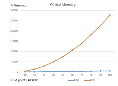
(a) Increasing number of clusters

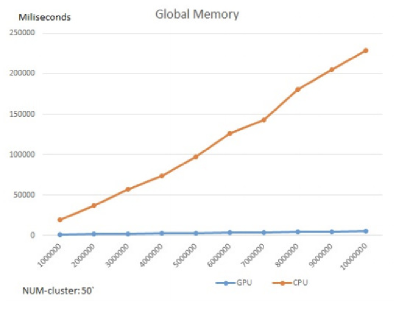
(b) Increasing number of points

Figure 1: Improvement over performance using Global Memory

We demonstrate the results for applying Global memory in our implementation. Using Global memory, we consider two scenarios: First, we discuss the improvements over GPU using Global memory rather than CPU when the number of points is increasing from 1 million to 10 million points, and the number of clusters is equivalent to a constant number (NumC = 50). Second, we explain the scenario when the number of clusters is increasing from 10 to 100 clusters, while the number of points is equal to a constant number (NumP = 4000000). In Fig. 1a and Fig. 1b, the results of using Global memory in abovementioned scenarios are indicated. As it is shown in Fig. 1, the performance of K-means++ algorithm has been amended when it is implemented over GPU than CPU. We can see more improvement when the number of points and clusters are increased gradually. Using Global memory, when the number of clusters grows from 10 to 100, GPU time varies between 1-5 while CPU time increases from 3 seconds to 4 minutes.

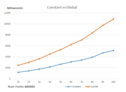
(a) Increasing number of clusters

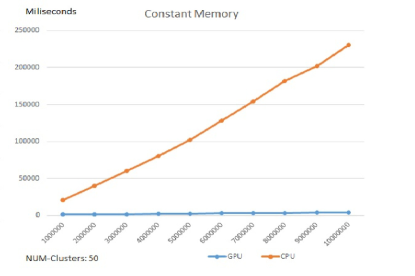
(b) Increasing number of points

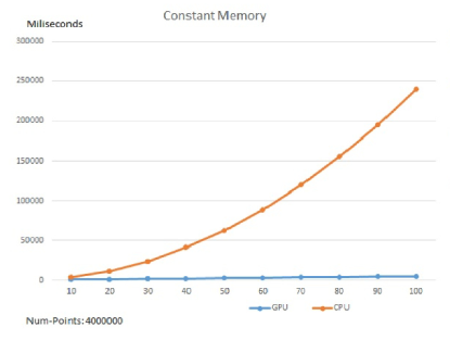
(c) Global vs Constant Memory

Figure 2: Improvement over performance using Constant Memory

On the other hand, increasing the number of points from 1-10 million, the GPU time changes within a range from 1-5 seconds while this time for the CPU version is from 18 seconds to 3 minutes. Next to Global memory, Fig. 2a and Fig. 2b, demonstrate the performance of the algorithm in parallel mode when we use Constant memory. As it is shown in Fig. 2, using Constant memory, we have a piecemeal improvement in the performance of the algorithm. Increasing the number of clusters from 1 to 100, the GPU time changes within a range between 1-5 seconds while this time for CPU is between 3 seconds to 4 minutes. In case of growth from 1 to 10 million points, the GPU time is 1-5 seconds while the CPU time is 18 seconds to 3 minutes. One point that should be mentioned is that the performance of Constant memory and Global memory seems to be the same when we describe the time in seconds, however, this changes when we consider time in milliseconds. To better show this, in Fig.  2c we make a comparison between the performance of Constant memory and Global memory. As it is illustrated in Fig. 2c, using Constant memory can provide better performance for the K-means++ algorithm. Comparing Global to Constant memory and changing the clusters from 10-100 points, we have slight improvement from 2-11 percent during these steps. We can even see better improvements when the number of clusters is further increased.

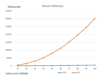
(a) Increasing number of clusters

(b) Increasing number of points

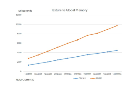
(c) Global vs Texture Memory

Figure 3: Improvement over performance using Texture Memory

Beside Global and Constant memory, we evaluate the proficiency of the K-means++ algorithm using Texture memory. We apply both of the aforementioned scenarios for this type of memory. Results are shown in Fig. 3. As it is indicated, using Texture memory, we have outstanding improvement and efficiency for the K-means++ algorithm. Incrementing number of clusters from 1 to 100 (Fig. 3a), the GPU time is within range roughly similar to Global memory and CPU time changes from 3 seconds to 4 minutes. In case of increasing the number of points from 1 million to 10 million (Fig. 3b), the GPU time changes between 1-4 seconds, which is slightly better than Global memory and the CPU time is the same as both Global and Constant memory. As we previously discussed, Texture memory can perform better when we are accessing neighbor locations in memory and because it is not modified from the device side. In Fig.  3c we provide the time comparison between Global memory and Texture memory. As it is presented, each time Texture memory is performing better, and at each step, Texture memory is between 10 to 14 percent more efficient in performance than global memory.

One result is expected. When the number of clusters is smaller, (K $<$ 7) the performance of CPU is slightly better than the GPU. This implies two things. First The data transfer from host to device and kernel launch overhead causes the GPU version takes longer. Second, we work in a two-dimensional environment. If the dimension is larger, we can easier reach to the point that GPU can provide better speed. As we can see, there is a trade-off between the speed of the algorithm and the required workload.

IV Conclusion

In this work, we provide a comprehensive study over parallelization of K-means++ algorithm. First, we describe the methodologies of parallelization, which were feasible for being implemented over the algorithm and talk about the ones which were impossible to be implemented. Second, we provide a detailed explanation over implementing each of these methodologies and the way we used in our methods. Finally, we evaluate our work when using any of these methodologies and make a comparison between them. Our results show the efficient performance of the algorithm over GPU rather than CPU. Also, it was demonstrated that in the case of our work, Constant memory and Texture memory had better efficacy than Global memory.

References

- [1] MacQueen, J., 1967, June. Some methods for classification and analysis of multivariate observations. In Proceedings of the fifth Berkeley symposium on mathematical statistics and probability (Vol. 1, No. 14, pp. 281-297).
- [2] Lloyd, S., 1982. Least squares quantization in PCM. IEEE transactions on information theory, 28(2), pp.129-137.Vancouver
- [3] Arthur, D. and Vassilvitskii, S., 2007, January. K-means++: The advantages of careful seeding. In Proceedings of the eighteenth annual ACM-SIAM symposium on Discrete algorithms (pp. 1027-1035). Society for Industrial and Applied Mathematics.
- [4] Hatamian, M., Ahmadpoor, S.S., Berenjian, S., Razeghi, B. and Barati, H., 2015, July. A centralized evolutionary clustering protocol for wireless sensor networks. In 2015 6th International Conference on Computing, Communication and Networking Technologies (ICCCNT) (pp. 1-6). IEEE.
- [5] Dhanachandra, N., Manglem, K. and Chanu, Y.J., 2015. Image segmentation using K-means clustering algorithm and subtractive clustering algorithm. Procedia Computer Science, 54, pp.764-771.
- [6] Guo, Q., Lu, X., Gao, Y., Zhang, J., Yan, B., Su, D., Song, A., Zhao, X. and Wang, G., 2017. Cluster analysis: a new approach for identification of underlying risk factors for coronary artery disease in essential hypertensive patients. Scientific reports, 7, p.43965.
- [7] Caron, M., Bojanowski, P., Joulin, A. and Douze, M., 2018. Deep clustering for unsupervised learning of visual features. In Proceedings of the European Conference on Computer Vision (ECCV) (pp. 132-149).
- [8] Berenjian, S., Shajari, M., Farshid, N. and Hatamian, M., 2016, September. Intelligent automated intrusion response system based on fuzzy decision making and risk assessment. In 2016 IEEE 8th International Conference on Intelligent Systems (IS) (pp. 709-714). IEEE.
- [9] Naghizadeh, A., Berenjian, S., Meamari, E. and Atani, R.E., 2016. Structural based tunneling: preserving mutual anonymity for circular P2P networks. International Journal of Communication Systems, 29(3), pp.602-619.
- [10] Naghizadeh, A., Berenjian, S., Razeghi, B., Shahanggar, S. and Pour, N.R., 2015, January. Preserving receiver’s anonymity for circular structured P2P networks. In 2015 12th Annual IEEE Consumer Communications and Networking Conference (CCNC) (pp. 71-76). IEEE.
- [11] Ng, R.T. and Han, J., 1994, September. Efficient and Effective clustering methods for spatial data mining. In Proceedings of VLDB (pp. 144-155).
- [12] T Zhang, R Ramakrishnan, M Livny, “BIRCH: an efficient data clustering method for very large databases”, in ACM SIGMOD international conference on Management of data, Volume 25 Issue 2, Pages 103-114, 1996.
- [13] Wang, M., Zhang, W., Ding, W., Dai, D., Zhang, H., Xie, H., Chen, L., Guo, Y. and Xie, J., 2014. Parallel clustering algorithm for large-scale biological data sets. PloS one, 9(4), p.e91315.
- [14] Kumar, J., Mills, R.T., Hoffman, F.M. and Hargrove, W.W., 2011. Parallel k-means clustering for quantitative ecoregion delineation using large data sets. Procedia Computer Science, 4, pp.1602-1611.
- [15] Mackey, P., Feo, J., Wong, P.C. and Chen, Y., 2011, April. A highly parallel implementation of k-means for multithreaded architecture. In Proceedings of the 19th High Performance Computing Symposia (pp. 33-39). Society for Computer Simulation International.
- [16] Zhang, J., Wu, G., Hu, X., Li, S. and Hao, S., 2011, December. A parallel k-means clustering algorithm with mpi. In 2011 Fourth International Symposium on Parallel Architectures, Algorithms and Programming (pp. 60-64). IEEE.
- [17] Karch, G., 2010. GPU based acceleration of selected clustering techniques [MS thesis].
- [18] Bahmani, B., Moseley, B., Vattani, A., Kumar, R. and Vassilvitskii, S., 2012. Scalable k-means++. Proceedings of the VLDB Endowment, 5(7), pp.622-633.
- [19] M. Harris, “An easy introduction to CUDA C and C++,” http://devblogs. nvidia.com/parallelforall/easy-introduction-cuda-c-and-c/, 2012.
- [20] NVIDIA Developer. (2019). CUDA Zone. [online] Available at: https://developer.nvidia.com/cuda-zone [Accessed 23 Jul. 2019].
- [21] Alvanos, M. and Christoudias, T., 2019. Accelerating Atmospheric Chemical Kinetics for Climate Simulations. IEEE Transactions on Parallel and Distributed Systems.
- [22] Bustamam, A., Burrage, K. and Hamilton, N.A., 2012. Fast parallel Markov clustering in bioinformatics using massively parallel computing on GPU with CUDA and ELLPACK-R sparse format. IEEE/ACM Transactions on Computational Biology and Bioinformatics (TCBB), 9(3), pp.679-692.
- [23] Li, C.Y. and Chang, H.H., 2017, February. CUDA-based acceleration of collateral filtering in brain MR images. In Eighth International Conference on Graphic and Image Processing (ICGIP 2016) (Vol. 10225, p. 1022528). International Society for Optics and Photonics.
- [24] Al-Ayyoub, M., AlZu’bi, S., Jararweh, Y., Shehab, M.A. and Gupta, B.B., 2018. Accelerating 3D medical volume segmentation using GPUs. Multimedia Tools and Applications, 77(4), pp.4939-4958.
- [25] Hernandez-Gutierrez, E., Ramirez-Manzanares, A., Marroquin, J.L., Ocampo-Pineda, M. and Daducci, A., 2019, April. Cuda Parallelization of Commit Framework for Efficient Microstructure-Informed Tractography. In 2019 IEEE 16th International Symposium on Biomedical Imaging (ISBI 2019) (pp. 1606-1609). IEEE.
- [26] NVidia, Thrust quick start guide, http://docs.nvidia.com/cuda/pdf/ Thrust Quick Start Guide.pdf, 2014.