The First fm/c of Heavy-Ion Collisions

Abstract

We present an introductory review of the early time dynamics of high-energy heavy-ion collisions and the kinetics of high temperature QCD. The equilibration mechanisms in the quark-gluon plasma uniquely reflect the non-abelian and ultra-relativistic character of the many body system. Starting with a brief expose of the key theoretical and experimental questions, we provide an overview of the theoretical tools employed in weak coupling studies of the early time non-equilibrium dynamics. We highlight theoretical progress in understanding different thermalization mechanisms in weakly coupled non-abelian plasmas, and discuss their relevance in describing the approach to local thermal equilibrium during the first ${\rm fm}/c$ of a heavy-ion collision. Some important connections to the phenomenology of heavy-ion collisions are also briefly discussed.

1 Introduction and motivation

The purpose of ultra-relativistic heavy ion collisions is to produce and to characterize the properties of the Quark-Gluon-Plasma (QGP), which is an extreme state of Quantum-Chromo-Dynamic (QCD) matter that was also present in the early universe, during the first mircoseconds after the big bang. Over the last two decades, experiments at the Relativistic Heavy-Ion Collider (RHIC) and the Large Hadron Collider (LHC) have collided a variety of nuclei over a wide range of energies, and, at least in the collisions of large nuclei, these experiments show that the produced constituents re-interact, and exhibit multi-particle correlations with wavelengths which are long compared to the microscopic correlation lengths, providing overwhelming evidence of collective hydrodynamic flow [1]. Hydrodynamic simulations of these large nuclear systems describe the observed correlations in exquisite detail with a minimal number of parameters [1]. In smaller systems such as proton-proton (pp) and proton-nucleus (pA) long range flow-like correlations amongst the produced particles have also been observed [2, 3], and these observations drive current research into the equilibration mechanism of the QGP. This research aims to understand how the observed correlations change with system size, and approach the hydrodynamic regime for large nuclei.

Explaining approximately how an equilibrated state of quarks and gluons emerges from the initial wave functions of the incoming nuclei has been one of the central goals of the heavy ion theory community for a long time. Even though genuinely non-perturbative real-time QCD calculations are currently not available to address this question (as they suffer from a severe sign problem), significant progress has been achieved in understanding properties of the initial state and the equilibration mechanism based on ab-initio calculations at weak and strong coupling. Here we focus on the weak coupling description, based on the idea that at high energy density and temperatures the coupling constant between quarks and gluons $\alpha_{s}$ becomes small, and weak coupling methods can be used to analyze the initial production of quarks and gluons, and the kinetic processes which ultimately lead to a thermalized QGP. When extrapolated to realistic coupling strength, the weak coupling approach based on perturbative QCD and strong-coupling approaches based on the holography yield similar results for the macroscopic evolution of the system [5]. For a recent review of the strong coupling description we refer to [4].

The weakly coupled picture of the equilibration process in high energy collisions was outlined in a seminal paper by Baier, Mueller, Schiff and Son (BMSS) [6], and is referred to as the bottom-up thermalization scenario,which is schematically depicted in Fig. 2. We provide a short review of bottom-up in Sect. 2, and then describe recent reanalyses which have clarified and extended the original picture considerably. These extensions have turned the parametric estimates of BMSS into hard numbers, which can be used to make contact with the experimental data.

We emphasize that the study of the equilibration mechanisms in non-abelian gauge theories, such as QCD, is of profound theoretical interest, and much of the research into thermalization is only tangentially driven by the immediate needs of experimental heavy ion physics program. In this spirit this review aims to cover some of the most important theoretical developments regarding the equilibration mechanism in non-abelian plasmas. Starting with an introductory discussion of the basic physics picture of the early stages of high-energy heavy-ion collisions in Sect. 2, the subsequent sections, Sects. 3 and 4, provide a more detailed theoretical discussion of the underlying theory and the equilibration process of weakly coupled non-abelian plasmas. New developments based on microscopic simulations and connections to heavy-ion phenomenology are then discussed in Sect. 5.

2 Early time dynamics of heavy-ion collisions

When two nuclei collide at high energies, they pass through each other scarcely stopped, leaving behind a debris of highly excited matter which continues to expand longitudinally [7]. Since the system is approximately invariant under boosts in the longitudinal ($z$) direction, one point functions of the stress tensor and other fields in the central rapidity region, i.e. the region close to the original interaction point, only depend on proper time $\tau=\sqrt{t^{2}-z^{2}}$, but do not depend on the space time rapidity $\eta=\tfrac{1}{2}\log((t+z)/(t-z))$. In co-moving $(\tau,x,y,\eta)$ coordinates, the metric is

$$ds^{2}=-d\tau^{2}+dx^{2}+dy^{2}+\tau^{2}d\eta^{2}\,,$$ (1)

indicating that the boost-invariant system is continually expanding along the beam axis, $dz=\tau\,d\eta$. While initially the system is in a state far from local thermal equilibrium, phenomenology suggests that on a time $\tau_{\text{hydro}}\sim 1\,{\rm fm/c}$ the plasma of quarks and gluons is sufficiently close to equilibrium that hydrodynamic constitutive relations are approximately satisfied and the subsequent evolution can be described with hydrodynamics.

While the longitudinal structure is approximately homogenous in space time rapidity, the transverse structure of the fireball is always inhomogenous, reflecting the initial geometry of the collision. In Fig. 1 we show a typical transverse (entropy density) profile that is used to initialize hydrodynamic simulations of the space time evolution. While the average geometry is characterized by the nuclear radius $R_{A}$, one finds that in any realistic event-by-event simulation there are smaller length scales in the initial geometry of order the proton radius, $R_{p}\ll R_{A}$, which arise from fluctuations in the positions of the incoming protons. Such geometric fluctuations are responsible for many of the most prominent flow observables in heavy ion collisions such as e.g. the triangular flow [8]. Still smaller fluctuations of order the inverse saturation momentum $Q_{s}^{-1}$ (see Sect. 2.1) are not shown in this figure. Different scales in Fig. 1 should be compared to the distance scale $c\tau_{\text{hydro}}$, which provides an estimate of the causal propagation distance during the approach to equilibrium. We will generally assume that $c\tau_{\text{hydro}}$ is short compared to the nuclear radius, $c\tau_{\text{hydro}}\ll R_{A}$, such that on average the transition from the non-equilibrium state towards thermal equilibrium proceeds locally in space and can discussed at the level of individual cells of size $c\tau_{\text{hydro}}$. Short distance fluctuations on scales $c\tau_{\text{hydro}}$ spoil this picture; however such effects were neglected in the original bottom-up scenario and we will follow this assumption by approximating the evolution of the system as homogenous in transverse space and space time rapidity throughout most of this review. Shortcomings of this approximation will be discussed further in Sec. 5 and 6 along with recent extensions of the original work of BMSS, which incorporate short distance fluctuations of the nucleon positions on scales $R_{p}\sim c\tau_{\text{hydro}}$ into the description of the first fm/c of heavy-ion collisions.

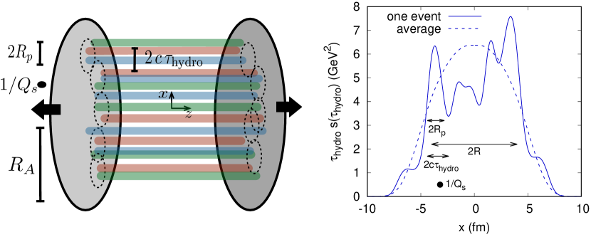
Figure 1: (left) Illustration of the two nuclei as they are passing through each other. Classical color field configurations just after passage were described in  [9, 10, 11] and feature strong longitudinal chromo-electric and chromo-magnetic fields, which rapidly decohere on a timescale of $\sim Q_{s}$ [12]. (right) Snapshot of a typical entropy density profile used in event-by-event hydrodynamic simulations of heavy-ion collisions [13]. Smaller scale fluctuations on microscopic length scales $\sim 1/Q_{s}$ are not shown, and are indicated by the black dot.

2.1 Microscopics of the initial state

In each small circle of size $c\tau_{\text{hydro}}$ in the transverse plane the initial production of quarks and gluons in momentum space follows from the Color-Glass-Condensate (CGC) effective theory of parton saturation [14, 15]. Briefly, in this theory the incoming nuclei are highly length contracted by an ultra-relativistic factor $\gamma\gg 1$, and the density of gluons per transverse area and rapidity in the wave functions of the nuclei, $(dN/dy)/\pi R_{A}^{2}$, grows with increasing collision energy. Here $dN/dy$ is the number of gluons per rapidity $y$ which is related to Bjorken $x_{\rm bj}$, $dy=dx_{\rm bj}/x_{\rm bj}$. This transverse density of gluons determines a momentum scale, known as the saturation momentum $Q_{s}$, which at very high energies can become large compared to $\Lambda_{\rm QCD}$

$$Q_{s}^{2}\sim\frac{\alpha_{s}}{\pi R_{A}^{2}}\frac{dN}{dy}\gg\Lambda_{QCD}^{2}\,.$$ (2)

The saturation momentum $Q_{s}$ sets the momentum scale for the transverse momentum distribution of partons in the wave functions. For $Q_{s}\gg\Lambda_{QCD}$ the coupling constant is small $\alpha_{s}(Q_{s})\ll 1$, and the evolution of the system can be treated using weakly coupled methods. Further, the number of gluons per phase space cell in the incoming wave functions is large

$$\frac{1}{\pi Q_{s}^{2}R_{A}^{2}}\frac{dN}{dy}\sim\frac{1}{\alpha_{s}}\gg 1\,,$$ (3)

and in this regime the evolution of the system is classical. Thus, the production of gluons and their initial evolution system is determined by solving the non-linear classical Yang-Mills equations of motion [9, 10, 11]. In practice, the saturation momentum is $Q_{s}\sim 1\,{\rm GeV}$ at RHIC and $2\,{\rm GeV}$ at the LHC. As these values not vastly larger than $\Lambda_{QCD}$ there will always be important quantum corrections to the CGC formalism, which will almost be completely neglected in this review.

In an important set of papers, the initial conditions for the classical fields in the forward light cone just after the intitial crossing of the two nuclei were worked out (analytically) by matching the classical fields just before the collision with those just after crossing [9, 10, 11]. These initial conditions consist of strong longitudinal fields, $E^{z}$ and $B^{z}$, which as illustrated in Fig. 1 is somewhat reminiscent of a parallel plate capacitor [12]. Indeed, the average stress tensor for a boost invariant, or Bjorken, expansion and a conformal system (with $T^{\mu}_{\;\mu}=0$) must take the form $\left\langle T^{\mu}_{\;\nu}\right\rangle=(-\epsilon,P_{T},P_{T},P_{L}),$ with $\epsilon=2P_{T}+P_{L}$. The matching procedure [9, 10, 11] shows that $\left\langle T^{\mu}_{\;\nu}\right\rangle=(-\epsilon,\epsilon,\epsilon,-\epsilon)$, and thus, the initial longitudinal “pressure” $P_{L}$ is negative as for a constant electric (or magnetic) field in the $z$-direction in classical electrodynamics. These strong longitudinal fields rapidly decrease on a time scale of $\sim Q_{s}$ as the classical field configuration decoheres.

The initial conditions outlined in the preceding paragraph motivated the first classical simulations of gluon production in the longitudinally expanding boost invariant geometry [16, 17]. In the original formulations the classical fields were assumed to remain effectively 2+1 dimensional, i.e. strictly independent of rapidity as a function of time $\tau$, reflecting the fact that the initial conditions are boost invariant up to quantum corrections of order $\alpha_{s}$. However, such quantum fluctuations provide the seed from which classical instabilities develop in the longitudinal direction [18, 8], such that the gluonic fields quickly become chaotic in all three dimensions and the classical solutions are only rapidity-independent on average. The instabilities grow as $~{}e^{\Gamma\sqrt{Q_{s}\tau}}$, with $\Gamma\sim 1$, limiting the applicability of strictly boost invariant simulations to short times, $\tau\lesssim Q_{s}^{-1}\,\log^{2}(1/\alpha_{s})$ [19, 20, 21]. In spite of this shortcoming, strictly boost invariant simulations of classical field dynamics form the basis of phenomenological studies of particle production and early time dynamics in the IP-Glasma model  [22, 23].

During the classical evolution the field strength decreases due to the longitudinal expansion, and eventually the equations of motion linearize. For times long enough $\tau Q_{s}\gg 1$ (but not too long; see Sect. 2.2) the phase space density of gluons is still large but much smaller than the inverse self-coupling $\alpha_{s}^{-1}(Q_{s})$. In this regime, either kinetic theory or classical field theory can be used to simulate the evolution of the system [24, 25, 26]. In particular, it is sensible to talk about the gluon phase space distribution, as opposed to the classical field configuration. The initial phase space distribution of gluons $f(\tau,{\bm{x}},{\bm{p}})$ can be determined from the classical simulations by evaluating the Wigner transform of equal time two point functions of gauge fields, after fixing a physical gauge such as the Coulomb Gauge (see for instance LABEL:Berges:2012ev,Berges:2013eia,Greif:2017bnr). Due to the longitudinal expansion of the system, the initial phase-space distribution of the system is strongly squeezed with $\left\langle p_{\perp}^{2}\right\rangle\sim Q_{s}^{2}$ and $\left\langle(p^{z})^{2}\right\rangle\ll\left\langle p_{\perp}^{2}\right\rangle$.

2.2 Bottom-up equilibration

This highly anisotropic initial state provides the starting point for the bottom-up scenario, which is illustrated in Fig. 2. During the first classical phase of bottom up the phase space distribution becomes increasingly anisotropic as time progresses.

In the original bottom-up proposal, the longitudinal width of the phase space distribution $\left\langle p_{z}^{2}\right\rangle$ is determined by momentum diffusion, i.e. small angle scatterings amongst the hard particles. The diffusion process tries to increase the longitudinal width, but competes with the expansion of the system. This competition leads to a scaling solution for the phase space distribution $f(\tau,p_{z},p_{\perp})$ at late times $Q_{s}\tau\gg 1$, where the transverse and longitudinal momenta are of order

$$\left\langle p_{T}^{2}\right\rangle\sim Q_{s}^{2}\,,$$ (4a)

$$\left\langle p_{z}^{2}\right\rangle\sim \frac{Q_{s}^{2}}{(Q_{s}\tau)^{2/3}}\,.$$ (4b)

During the first stage of bottom-up, the number of hard gluons per rapidity remains constant $dN/dy\sim Q_{s}^{2}R_{A}^{2}/\alpha_{s}$, and thus the density of gluons (the number per volume) decreases as $n_{h}\sim Q_{s}^{2}/\alpha_{s}\tau$ due to the expansion of the system. Based on these estimates, the phase space density of hard modes decreases as

$$f_{h}\sim\frac{1}{\alpha_{s}}\frac{1}{(Q_{s}\tau)^{2/3}}\,,$$ (5)

following a pattern which is characteristic of overoccupied initial states with $f_{h}\gg 1$, which will be discussed in greater detail in Sect. 4.1 and Sect. 4.3. Analyzing eq. (5), we see that the phase space density becomes of order unity at a time of order $Q_{s}\tau\sim\alpha_{s}^{-3/2}$, marking the end of the first over-occupied stage. Most importantly, from this point onward the system can no longer be treated as a classical field, and its subsequent evolution must be analyzed with kinetic theory.

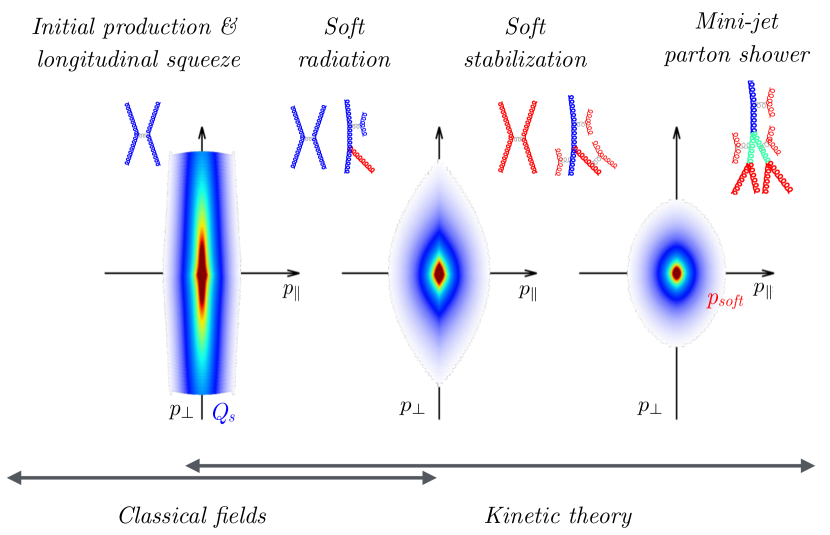
Figure 2: Schematic overview of the bottom-up thermalization showing the evolution of the phase-space distribution of gluons in momentum space based on kinetic theory simulations of  [30]. Different regimes correspond to evolution times $\tau/\tau_{\text{hydro}}\approx 0.1,~{}0.5,~{}1$ at realistic coupling strength $\alpha_{s}\approx 0.3$

In the second stage of bottom-up, $Q_{s}\tau\gg\alpha_{s}^{3/2}$, radiation from the hard modes increases the number of soft gluons per rapidity. Ultimately this soft bath will thermalize the hard modes giving the bottom-up equilibration scenario its name. While the soft bath is being populated, the number of hard particles per volume continues to decrease due to the longitudinal expansion, $n_{h}\sim Q_{s}^{2}/\alpha_{s}\tau$. Now, however, the longitudinal width $\left\langle p_{z}^{2}\right\rangle$ of these hard modes remains constant in time, since the increase in width from (momentum) diffusion is compensated for by the expansion of the system

$$\left\langle p_{T}^{2}\right\rangle\sim Q_{s}^{2}\,,$$ (6a)

$$\left\langle p_{z}^{2}\right\rangle\sim \alpha_{s}Q_{s}^{2}\,.$$ (6b)

Thus, the phase space density of hard particles in the second phase decreases as

$$f_{h}\sim\frac{1}{\alpha_{s}^{3/2}}\frac{1}{(Q_{s}\tau)}\,,\qquad Q_{s}\tau\gg\alpha_{s}^{-3/2}\,,$$ (7)

and is therefore much smaller than unity. Indeed, at the end of the second phase of bottom-up, $Q_{s}\tau\sim\alpha_{s}^{-5/2}$, the phase space density of the hard modes is parametrically small, $f_{h}\sim\alpha_{s}\ll 1$.

In the last stage of the bottom-up $Q_{s}\tau\gg\alpha_{s}^{-5/2}$ the soft bath has equilibrated, and begins to influence the evolution of the hard particles. In this stage there is a cascade of energy from the scale of $Q_{s}$ to the soft scale scale set by the temperature of the bath. The physics of this process is analogous to the stopping of “jets” with momentum of order $Q_{s}$ in plasma [6, 31, 32] and described further in Sect. 4.2 and Sect. 4.3.

The second and third stages of the bottom-up scenario are characteristic of the thermalization of initially under-occupied systems. We will see in Sect. 4.2 that the buildup of a soft thermal bath, and cascade of energy to the infrared are to be expected in such systems.

3 QCD Kinetics: a brief review

Having qualitatively described the bottom-up picture, we will now turn to a more quantitative analysis of the equilibration process of the QGP in the framework of kinetic theory. Kinetic processes in the QGP are markedly different from other many-body systems of condensed matter physics, uniquely reflecting the non-abelian and ultra-relativistic character of the produced quark and gluon quasi-particles. A complete leading order description of QCD kinetics (close to equilibrium) was given in [33], and was then used to compute the transport coefficients of the QCD plasma to leading order in the strong coupling constant [34].

Here we will provide a brief review of QCD kinetics to establish notation and to collect the principal results. If not stated otherwise we will focus on pure gauge systems, and refer to the literature for additional details [33, 35]. Further we will, at points, have to assume that the momentum distribution is isotropic; issues which arise in the description of anisotropic systems (such as plasma instabilities) will be discussed briefly in Sect. 4.3.

The QCD Boltzmann equation takes the form

$$\left(\partial_{t}+{\bm{v}}_{\bm{p}}\cdot\partial_{\bm{x}}\right)f(t,{\bm{x}},{\bm{p}})=C^{2\leftrightarrow 2}[f({\bm{p}})]+C^{1\leftrightarrow 2}_{\rm inel}[f({\bm{p}})]\,,$$ (8)

where the $2\leftrightarrow 2$ rates describes elastic scattering, and $C^{1\leftrightarrow 2}$ describes collinear radiation. We further introduce two dimensionful integrals

$$m^{2}\equiv \nu_{g}\frac{g^{2}C_{A}}{d_{A}}\int_{\bm{p}}\frac{f_{\bm{p}}}{p}\,,$$ (9)

$$2T_{*}m^{2}\equiv \nu_{g}\frac{g^{2}C_{A}}{d_{A}}\int_{\bm{p}}f_{\bm{p}}(1+f_{\bm{p}})\,.$$ (10)

to characterize the momentum distribution. Modes of order $m$ are considered soft, while modes of order $T_{*}$ are hard. In equilibrium $T_{*}$ is the temperature of the medium, and $m$ is the asymptotic mass of the gluon dispersion curve, i.e. $E_{\bm{p}}=\sqrt{{\bm{p}}^{2}+m^{2}}\simeq|{\bm{p}}|+m^{2}/2|{\bm{p}}|$.

3.1 Elastic scattering and momentum diffusion

The $2\leftrightarrow 2$ processes can be divided into soft collisions, where the momentum transfer is of order $m$ and screening is important, and hard collisions, where the momentum transfer is above a cutoff scale $\mu^{2}_{\perp}\sim T_{*}m$ and screening can be neglected:

$$C^{2\leftrightarrow 2}[f({\bm{p}})]=C_{\rm diff}[f({\bm{p}})]+C_{\rm hard}^{2\leftrightarrow 2}[f({\bm{p}})]\,.$$ (11)

Hard collisions (which are conceptually straightforward) exhibit the same parametric dependencies as soft interactions (see e.g. [36]) and will be ignored in the estimates below. Elastic interactions with soft momentum transfers create drag and diffusion processes in momentum space, which may be summarized by a Fokker-Planck equation. This separation into hard and soft collisions was essential to an almost complete next-to-leading-order computation of the shear viscosity [35].

Consider a particle of momentum ${\bm{p}}$ (with four velocity $v_{\bm{p}}^{\mu}\equiv(1,\hat{\bm{p}})$) being jostled by a soft random external field $A^{\mu}(Q)$ created by all other particles. The absorption rate of three momentum ${\bm{q}}$ by the field is

$$\frac{d\Gamma_{\rm el}^{>}(\hat{\bm{p}})}{d^{3}q}=g^{2}C_{A}\,\int\frac{dq^{0}}{2\pi}\,v_{\bm{p}}^{\mu}v_{\bm{p}}^{\nu}\;\langle\!\langle A_{\mu}(Q)\,(A_{\nu}(Q))^{*}\rangle\!\rangle^{>}\;2\pi\delta(v_{\bm{p}}\cdot Q)\,,$$ (12)

where the $\delta$-function stems from energy conservation, $2\pi\delta(q^{0}+E_{{\bm{p}}-{\bm{q}}}-E_{\bm{p}})\simeq 2\pi\delta(v_{\bm{p}}\cdot Q)$. Statistical fluctuations of the gauge field fluctuations are given by

$$\langle\!\langle A^{\mu}(Q)(A^{\nu}(Q))^{*}\rangle\!\rangle^{>}=G_{R}^{\mu\alpha}(Q)\,\Pi^{>}_{\alpha\beta}(Q)\,(G_{R}^{\beta\nu}(Q))^{*}\,,$$ (13)

where the Wightman self energy reads

$$(\Pi^{>}(Q))^{\alpha\beta}= \nu_{g}\frac{g^{2}C_{A}}{d_{A}}\int_{{\bm{k}}}\,v_{{\bm{k}}}^{\alpha}v_{{\bm{k}}}^{\beta}\,f({\bm{k}})(1+f({\bm{k}}+{\bm{q}}))\,2\pi\delta(v_{\bm{k}}\cdot Q)\,,$$ (14)

Here $G_{R}(Q)\sim 1/Q^{2}$ is the hard thermal loop retarded response function [37], which can only be worked out in closed form for isotropic systems. In the limit of small ${\bm{q}}$ the population factors in eq. (14) become $f({\bm{k}})(1+f({\bm{k}}))$, and the correlator in eq. (13) has a simple interpretation – it is the correlation amongst the gauge fields $A=(G_{R}(Q))\cdot\,gv_{{\bm{k}}}$ produced by random fluctuations of the phase space density $\delta f(t,{\bm{x}},{\bm{k}})$, which have the usual equal time Bose-Einstein statistics [38]

$$\langle\!\langle\delta f(t,{\bm{x}},{\bm{k}})\,\delta f(t,{\bm{x}}^{\prime},{\bm{k}})\rangle\!\rangle=f(t,{\bm{x}},{\bm{k}})\,(1+f(t,{\bm{x}},{\bm{k}}))\,\delta^{3}({\bm{x}}-{\bm{x}}^{\prime})\,(2\pi)^{3}\delta^{3}({\bm{k}}-{\bm{k}}^{\prime})\,.$$ (15)

The absorption rate in eq. (12) gives the rate that momentum ${\bm{q}}$ is taken from the particle and given to the bath. Similarly, the emission rate takes the same form as eq. (12) but replaces the self energy $\Pi^{>}$ with

$$(\Pi^{<}(Q))^{\alpha\beta}=\nu_{g}\frac{g^{2}C_{A}}{d_{A}}\int_{\bm{k}}v_{\bm{k}}^{\alpha}v_{\bm{k}}^{\beta}\,f({\bm{k}}+{\bm{q}})(1+f({\bm{k}}))\,2\pi\delta(v_{\bm{k}}\cdot Q)\,,$$ (16)

such that at small ${\bm{q}}$ the emission and absorption rates are equal, and it is the symmetric correlator $\Gamma_{\rm{\scriptscriptstyle\mathrm{el}}}{=}(\Gamma^{>}_{\rm{\scriptscriptstyle\mathrm{el}}}+\Gamma_{\rm{\scriptscriptstyle\mathrm{el}}}^{<})/2$ that will determine the rates of momentum diffusion below. Conversely, the difference in the emission and absorption rates determines the drag, and involves:

$$(\Pi^{>}(Q)-\Pi^{<}(Q))^{\alpha\beta}= \nu_{g}\frac{g^{2}C_{A}}{d_{A}}\int_{\bm{k}}\,v_{\bm{k}}^{\alpha}v_{\bm{k}}^{\beta}\;q^{i}\frac{\partial f({\bm{k}})}{\partial k^{i}}\,2\pi\delta(v_{\bm{k}}\cdot Q)\,,$$ (17)

$$= 2q^{0}\,m^{2}\int\frac{d\Omega}{4\pi}\,v_{{\bm{k}}}^{\alpha}v_{\bm{k}}^{\beta}\,2\pi\delta(v_{\bm{k}}\cdot Q)\,,$$ (18)

where in passing to the last line we have assumed that the system is isotropic, $\partial f/\partial k^{i}=f^{\prime}(k)\hat{k}^{i}$, allowing us to perform an integration by parts.

The evolution of the system due to soft scattering is a competition between the emission and absorption rates

$$\partial_{t}f_{\bm{p}}+{\bm{v}}_{\bm{p}}\cdot\partial_{\bm{x}}f_{\bm{p}}=\int{\rm d}^{3}q\,\left(\frac{{\rm d}\Gamma_{\rm el}^{<}(\hat{\bm{p}})}{{\rm d}^{3}q}\,f_{{\bm{p}}-{\bm{q}}}(1+f_{\bm{p}})-\frac{{\rm d}\Gamma_{\rm el}^{>}(\hat{\bm{p}})}{{\rm d}^{3}q}\,f_{\bm{p}}(1+f_{{\bm{p}}-{\bm{q}}})\right)\,.$$ (19)

We will now generally assume that the distribution is isotropic which simplifies the analysis of momentum diffusion. Expanding in powers of the momentum transfer ${\bm{q}}$ (which is small compared to the momentum ${\bm{p}}$ of the hard particle), we see that the contribution of small angle elastic processes to the Boltzmann equation (8) takes the form of a Fokker-Planck equation

$$C_{\rm diff}[f({\bm{p}})]=\eta^{i}(\hat{\bm{p}})\frac{\partial}{\partial p^{i}}\left(f_{\bm{p}}(1+f_{\bm{p}})\right)+\hat{q}^{ij}(\hat{\bm{p}})\frac{\partial^{2}f_{\bm{p}}}{\partial p^{i}\partial p^{j}}\,,$$ (20)

where the drag and diffusion coefficients are given by

$$\eta^{i}= \int{\rm d}^{3}q\left(\frac{{\rm d}\Gamma^{>}_{\rm el}(\hat{\bm{p}})}{{\rm d}^{3}q}-\frac{{\rm d}\Gamma^{<}_{\rm el}(\hat{\bm{p}})}{{\rm d}^{3}q}\right)q^{i}\,,$$ (21)

$$\hat{q}^{ij}(\hat{\bm{p}})= \int d^{3}q\,\left(\frac{{\rm d}\Gamma_{\rm el}(\hat{\bm{p}})}{{\rm d}^{3}q}\right)q^{i}q^{j}\,.$$ (22)

Specifically for isotropic systems these coefficients can be decomposed as

$$\eta^{i}(\hat{\bm{p}})=\eta\hat{p}^{i}\,,\qquad q^{ij}(\hat{\bm{p}})=\hat{q}_{L}\hat{p}^{i}\hat{p}^{j}+\tfrac{1}{2}\hat{q}\left(\delta^{ij}-\hat{p}^{i}\hat{p}^{j}\right)\,,$$ (23)

and the scalar coefficients $\eta,\hat{q}_{L},\hat{q}$ can be evaluated as (see [39] for a review),

$$\eta= \frac{g^{2}C_{A}m^{2}}{8\pi}\log\left(\frac{\mu_{\perp}^{2}}{m^{2}}\right)\,,$$ (24a)

$$\hat{q}_{L}= \frac{g^{2}C_{A}\,(2T_{*}m^{2})}{8\pi}\log\left(\frac{\mu_{\perp}^{2}}{m^{2}}\right)\,,$$ (24b)

$$\hat{q}= \frac{g^{2}C_{A}\,(2T_{*}m^{2})}{4\pi}\log\left(\frac{\mu_{\perp}^{2}}{2m^{2}}\right)\,.$$ (24c)

Similarly, the elastic scattering rate for kicks transverse to the direction of the particle can also be evaluated in closed form yielding

$$(2\pi)^{2}\frac{d\Gamma_{\rm el}}{d^{2}q_{\perp}}=g^{2}C_{A}T^{*}\left(\frac{1}{q_{\perp}^{2}}-\frac{1}{q_{\perp}^{2}+2m^{2}}\right)\,.$$ (25)

Although the Fokker-Planck coefficients in eq. (24a) depend on the cutoff scale $\mu_{\perp}$, the time the evolution of the system is independent of $\mu_{\perp}$, when both the hard collisions and the Fokker-Planck evolution are taken into account [40]. We finally note that from eq. (25) and eq. (24c), the elastic scattering rate is of order

$$\Gamma_{\rm el}\sim\int_{\sim m}{\rm d}^{2}q_{\perp}\frac{{\rm d}\Gamma_{\rm el}}{{\rm d}^{2}q_{\perp}}\sim\frac{\hat{q}}{m^{2}}\,,$$ (26)

which will be used repeatedly when estimating the rate of collinear radiation described in the next section.

3.2 Collinear radiation

Elastic scatterings of ultra-relativistic particles induce collinear radiation as the charged particles are accelerated by the random kicks from the plasma. A massless gluon with momentum ${\bm{P}}={\bm{p}}+{\bm{k}}$ can split into two particles with momentum fractions $z$ and $\bar{z}\equiv(1-z)$, where ${\bm{p}}=z{\bm{P}}$ and ${\bm{k}}=\bar{z}{\bm{P}}$ respectively. These radiative process should be incorporated into the Boltzmann equation at leading order [6, 33]. Denoting the rate for this process as ${\rm d}\Gamma_{\rm inel}({\bm{P}})/{\rm d}z$, the contribution to the Boltzmann equation can be written as

$$C^{1\leftrightarrow 2}[f({\bm{p}})]= \nu_{g}\int_{{\bm{P}}}\int_{0}^{1}dz\,\frac{{\rm d}\Gamma_{{\scriptscriptstyle\mathrm{inel}}}({\bm{P}})}{{\rm d}z}\,\frac{(2\pi)^{3}}{\nu_{g}}\delta^{(3)}({\bm{p}}-z{\bm{P}})\,$$

$$\qquad\times\left[f({\bm{P}})(1+f(z{\bm{p}}))(1+f(\bar{z}{\bm{P}}))-f(z{\bm{P}})f(\bar{z}{\bm{P}})(1+f({\bm{P}}))\right]$$

$$- \frac{1}{2}\int_{0}^{1}dz\frac{d\Gamma_{{\scriptscriptstyle\mathrm{inel}}}({\bm{p}})}{dz}$$

$$\qquad\times\left[f({\bm{p}})(1+f(z{\bm{p}}))(1+f(\bar{z}{\bm{p}}))-f(z{\bm{p}})f(\bar{z}{\bm{p}})(1+f({\bm{p}}))\right]\,,$$ (28)

and we will now briefly describe the characteristic features of the splitting rate.

In the splitting process the energy difference between the incoming and outgoing states is

$$\delta E= E_{\bm{p}}+E_{\bm{k}}-E_{{\bm{p}}+{\bm{k}}}\simeq\frac{h^{2}}{2Pz(1-z)}+\frac{m^{2}}{2Pz}+\frac{m^{2}}{2P(1-z)}-\frac{m^{2}}{2P}\,,$$ (29)

where ${\bm{h}}\equiv z{\bm{k}}_{\perp}-(1-z){\bm{p}}_{\perp}$ is essentially the transverse momentum of the softest fragment. In writing eq. (29) we have expanded the quasiparticle energy for small transverse momentum, $E_{\bm{p}}\simeq p^{z}+(m^{2}+p_{\perp}^{2})/2p$. Since the Hamiltonian time evolution of the system involves phases of the form $e^{-i\delta Et}$, the splitting process is only completed on a time scale

$$t_{\rm form}\equiv\frac{1}{\delta E}\,.$$ (30)

which defines an important timescale for collinear radiation, namely the formation time.

For highly energetic particles the formation time can become long compared to the time between elastic collisions. In this regime multiple scattering will suppress the emission of gluon radition, and this suppression is known as the Landau-Pomenanchuk-Migdal (LPM) effect.

Let us estimate the energy $\omega_{{\scriptscriptstyle\rm LPM}}$ when the LPM effect becomes operative, i.e. when $t_{\rm form}\Gamma_{\rm el}\sim 1$. To this end, consider a splitting process with $z\ll 1$ , so that $h\simeq p_{\perp}$ and $p=zP\sim\omega_{{\scriptscriptstyle\rm LPM}}$. In this regime the formation time is of order

$$t_{\rm form}\sim\frac{2p}{p_{\perp}^{2}}\sim\frac{\omega_{\scriptscriptstyle\rm LPM}}{m^{2}}\,,$$ (31)

were we have estimated $p_{\perp}^{2}\sim m^{2}$ as the typical momentum associated with a single elastic scattering event. Since the elastic scattering rate is of order $\Gamma_{\rm el}\sim\hat{q}/m^{2}$, we find

$$\omega_{{\scriptscriptstyle\rm LPM}}\sim\frac{m^{4}}{\hat{q}}\,.$$ (32)

For high energy particles the formation time becomes much longer than $\Gamma_{\rm el}^{-1}$. In this limit the accumulated transverse momentumg grows as $h^{2}\sim\hat{q}\,t_{\rm form}\gg m^{2}$, and thus using eq. (30) and eq. (29) we find the following estimate for the formation time

$$t_{\rm form}\sim\sqrt{\frac{P}{z(1-z)\hat{q}}}\,.$$ (33)

For $\omega\gtrsim\omega_{{\scriptscriptstyle\rm LPM}}$ the radiation rate must account for the multiple scatterings that happen during the formation time of the radiation. Conversely, in the Bethe-Heitler (BH) limit $\omega\ll\omega_{{\scriptscriptstyle\rm LPM}}$, the interference between the scattering events can be neglected, and each scattering has a probability of order $\alpha$ to radiate a gluon with momentum fraction $z$ disributed according to the splitting function $P_{g\rightarrow g}(z)$. Since the scattering rate is $\Gamma_{\rm el}\sim\hat{q}/m^{2}$, the total splitting rate in the BH limit is of order

$$\frac{{\rm d}\Gamma_{\rm inel}^{{\scriptscriptstyle\rm BH}}({\bm{p}}_{0})}{{\rm d}z}\sim\alpha\,P_{g\rightarrow g}^{\rm soft}(z)\,\frac{\hat{q}}{m^{2}}\,.$$ (34)

More generally emissions radiated within a formation time will destructively interfere, and the net emission rate is determined by solving an integral equation. This rate takes the form [43, 44, 6, 33, 41]

$$\frac{d\Gamma_{\rm{\scriptscriptstyle\mathrm{inel}}}({\bm{P}})}{{\rm d}z}=\alpha_{s}P_{g\rightarrow g}(z)\int\frac{d^{2}h}{(2\pi)^{2}}\,\frac{2{\bm{h}}\cdot\text{Re}{\bm{f}}({\bm{h}})}{(2Pz(1-z))^{2}}\,,$$ (35)

where the integral in this equation has units $({\rm time})^{-1}$. The function ${\bm{f}}({\bm{h}})$ (which encodes the current-current statistical correlation function) satisfies an integral equation of the form

$$2{\bm{h}}= i\,\delta E(h)\,{\bm{f}}({\bm{h}})+\int d^{2}q_{\perp}\frac{d\Gamma_{{\scriptscriptstyle\mathrm{el}}}}{d^{2}q_{\perp}}\big{\{}{\tfrac{1}{2}}\left[{\bm{f}}({\bm{h}})-{\bm{f}}({\bm{h}}+{\bm{q}}_{\perp})\right]$$

$$\qquad\qquad+{\tfrac{1}{2}}\left[{\bm{f}}({\bm{h}})-{\bm{f}}({\bm{h}}+z{\bm{q}}_{\perp})\right]+{\tfrac{1}{2}}\left[{\bm{f}}({\bm{h}})-{\bm{f}}({\bm{h}}+(1-z){\bm{q}}_{\perp})\right]\big{\}}\,.$$ (36)

To analyze this equation, let us take the Bethe-Heitler limit when the radiation is soft, $z\ll 1$ and $\omega\ll\omega_{{\scriptscriptstyle\rm LPM}}$, so that the formation time is small compared to the elastic scattering rate, $\delta E\gg\Gamma_{\rm el}$. In this regime we can solve eq. (3.2) by iteration, ${\bm{f}}={\bm{f}}^{(0)}+{\bm{f}}^{(1)}+\ldots$, with ${\bm{f}}^{(0)}({\bm{h}})=-2i{\bm{h}}/\delta E(h)$. Physically this expansion corresponds to the number of collisions, with ${\bm{f}}^{(1)}$ determining the emission rate from one collision and so on. After straightforward algebra one finds

$$\frac{{\rm d}\Gamma_{\rm inel}^{{\scriptscriptstyle\rm BH}}({\bm{p}}_{0})}{{\rm d}z}=2\alpha_{s}\,P_{g\rightarrow g}^{\rm soft}(z)\,\int\frac{d^{2}p_{\perp}}{(2\pi)^{2}}\int d^{2}q_{\perp}\frac{d\Gamma_{\rm el}}{d^{2}q_{\perp}}\left(\frac{{\bm{p}}_{\perp}}{p_{\perp}^{2}+m^{2}}-\frac{{\bm{p}}_{\perp}+{\bm{q}}_{\perp}}{({\bm{p}}_{\perp}+{\bm{q}}_{\perp})^{2}+m^{2}}\right)^{2}\,.$$ (37)

The large ${\bm{p}}_{\perp}$ limit of this rate is known as the Gunion-Bertsch formula [45]

$$(2\pi)^{2}\frac{{\rm d}\Gamma_{\rm inel}^{{\scriptscriptstyle\rm BH}}({\bm{P}})}{{\rm d}z\,{\rm d}^{2}p_{\perp}}=2\alpha_{s}\,P_{g\rightarrow g}^{\rm soft}(z)\,\frac{\hat{q}}{p_{\perp}^{4}}\,.$$ (38)

To estimate the total rate one can integrate this expression over $p_{\perp}$ down to a scale $p_{\perp}\sim m$ yielding the Bethe-Heitler estimate given earlier in eq. (34) .

In the opposite limit $\omega\gg\omega_{LPM}$ we can also find an approximate solution to eq. (3.2) known as the harmonic oscillator approximation. Since for $\omega\gg\omega_{LPM}$ the transverse momentum $h$ acquired over the formation time is large compared to the typical momentum transfer $q_{\perp}$ aquired in a single scattering $q_{\perp}\sim m$, one can expand the differences ${\bm{f}}({\bm{h}})-{\bm{f}}({\bm{h}}+{\bm{q}}_{\perp})$ for small ${\bm{q}}_{\perp}$, which transforms (3.2) into a partial differential equation

$$2{\bm{h}}=i\delta E(h){\bm{f}}({\bm{h}})-\frac{1+z^{2}+(1-z)^{2}}{8}\,\hat{q}\,\delta^{ij}_{\perp}\frac{\partial^{2}}{\partial h^{i}\,\partial h^{j}}{\bm{f}}({\bm{h}})$$ (39)

By approximating $\delta E(h)\simeq\frac{h^{2}}{2Pz(1-z)}$ and Fourier transforming with respect to ${\bm{h}}$ (with ${\bm{b}}$ conjugate to ${\bm{h}}$), one obtains a Schrödinger-like equation for a particle with an effective mass $M=Pz(1-z)$ in an imaginary harmonic potential $V({\bm{b}})=\tfrac{-i}{2}M\omega_{0}^{2}{b}^{2}$ with oscillation frequency $\omega_{0}^{2}=\hat{q}\frac{1+z^{2}+(1-z)^{2}}{4z(1-z)P}$. Solving this equation, one finds that the final emission rate is proportional to $\omega_{0}\sim t_{\rm form}^{-1}$, which in the soft limit $(z\ll 1)$ yields

$$\frac{d\Gamma_{\rm inel}^{{\scriptscriptstyle\rm LPM}}({\bm{P}})}{dz}= \frac{\alpha_{s}}{2\pi}\;P_{g\rightarrow g}^{\rm soft}(z)\;\sqrt{\frac{\hat{q}}{Pz(1-z)}}\,.$$ (40)

General expressions for the emission rates involving multiple species are given in [46, 42] in the same notation used here. Comparing eq. (40) with the Bethe-Heitler limit of eq. (34), shows that the emission rate is controlled by the inverse of the formation time $1/t_{\rm form}$ rather than the elastic scattering rate $\sim\hat{q}/m^{2}$ in eq. (34), suppressing the emission of radiation at high energies.

4 Basics of weak coupling thermalization

Now that we have outlined the basic physics of QCD kinetics, we will illustrate key features of the equilibration process in homogenous isotropic systems where a detailed understanding of the dynamics has been gained in a series of studies [36, 47, 48, 49]. Since the equilibration dynamics crucially depends on the properties of the initial state, it useful to distinguish between systems which are initially far from equilibrium, and systems which are initially close equilibrium. While in the latter case, one expects a direct relaxation of the system to equilibrium governed by an equilibrium rate, the situation is more complicated for systems which are initially far from equilibrium, and various kinds of phenomena can occur en-route towards thermal equilibrium. Nevertheless a general characterization of the equilibration process can be achieved for broad classes of far from equilibrium initial conditions. Specifically, for homogenous and isotropic systems one needs to distinguish between overoccupied systems, i.e. systems in which the energy is initially carried by a large number of low energy degrees of freedom, and underoccupied systems, i.e. systems in which the energy is carried by a small number of very high energy degrees of freedom. As we have emphasized in the previous section the first stage of the bottom-up scenario corresponds to the “over-occupied” case, while the second and third stages correspond to the under-occuppied case.

4.1 Overoccupied systems

We first consider a system where the initial energy density is carried by a large number of low energy degrees of freedom, i.e. if the quasi-particle energy is $E_{\bm{p}}\sim Q$, then the energy density is $e\sim f_{0}Q^{4}$ where $f_{0}\gg 1$ denotes the initial phase-space density. Clearly, this initial state is very far from an equilibrium state, where the energy density $e_{\rm eq}\sim T^{4}$ is carried by a smaller number of modes with $f\sim 1$ and $E_{\bm{p}}\sim T$. Since energy is conserved during the evolution, the final temperatue $T\sim Q\,f_{0}^{1/4}$ at the end of the equilibration process is much larger than $Q$. Because of this large scale separation between $Q$ and $T$, the redistribution of energy from low energy modes to high energy modes is then a classic problem of turbulence known as a direct energy cascade discussed in the next section [50].

4.1.1 Non-thermal fixed points and the energy cascade

The initial evolution of overoccupied plasmas can be equivalently described in terms of classical fields or weakly interacting quasi particles, due to an overlap in their respective range of validity [24, 25, 26]. For this reason the initial evolution can either be studied using classical-statistical simulations of the non-linear gauge field dynamics (see e.g. [48]), or using the numerical simulations and analytic considerations of kinetic theory [36, 47].

It was found that the initial evolution of overoccupied systems proceeds via a quasi-stationary state referred to as a non-thermal fixed point (NTFP). Here the dynamics becomes insensitive to the details of the initial conditions after a short time, and the evolution follows a self-similar scaling behavior [51, 52, 48]. Indeed, the phase-space density $f(t,{\bm{p}})$ in this regime evolves with the scaling form

$$f(t,{\bm{p}})=(Qt)^{\alpha}f_{S}\left((Qt)^{\beta}\frac{p}{Q}\right)\;,$$ (41)

which is characteristic for non-stationary turbulent processes [50] and the scaling form in eq. (41) describes a direct energy cascade, i.e. the transport of energy from low momentum to high momentum excitations necessary to achieve thermalization.

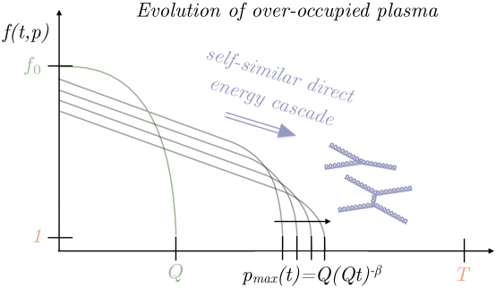
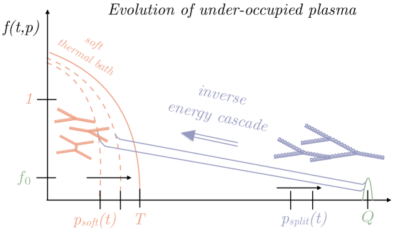
Figure 3: Illustration of the thermalization process in over-occupied and under-occupied systems, summarizing the results of classical-statistical field simulations[52, 51, 48] and kinetic theory simulations [53, 49].

The scaling exponents $\alpha,\beta$ (which will be negative) determine the increase of the characteristic momentum scale $p_{\rm max}(t)\sim Q(Qt)^{-\beta}$, and the simultaneous decrease of the occupancy of hard excitations $f(t,p\sim p_{\rm max}(t))\sim(Qt)^{\alpha}$ (see Fig. 3). These scaling exponents can be determined from a straightforward scaling analysis of the underlying kinetic equations [47, 36, 51, 48] following well established techniques in the context of weak wave turbulence [50]. One immediate constraint on the scaling exponents $\alpha,\beta$ comes from the requirement of energy conservation

$$e(t)=\int_{{\bm{p}}}E_{{\bm{p}}}\,f(t,{\bm{p}})=\textrm{const},$$ (42)

which for a self-similar evolution of the form in eq. (41) gives rise to a scaling relation

$$\alpha-4\beta=0\;.$$ (43)

A second scaling relation can be inferred from a scaling analysis of the kinetic equation. Even though the full scaling analysis of all leading order kinetic processes is somewhat complicated, the essence can be understood by considering as an example small angle elastic processes, whose contribution to the collision integral in eq. (20) is of the form of a Fokker-Planck equation, where the drag coefficient $\eta(t)$ and momentum diffusion coefficient $\hat{q}(t)$ are of order (see eq. (24) and eq. (9))

$$\eta(t)\sim \alpha^{2}_{s}\int_{{\bm{p}}}\frac{f(t,{\bm{p}})}{p}\,,$$ (44a)

$$\hat{q}(t)\sim \alpha^{2}_{s}\int_{{\bm{p}}}f(t,{\bm{p}})\,(1+f(t,{\bm{p}}))\,.$$ (44b)

With the scaling ansatz of eq. (41) in the high-occupancy regime $f(t,{\bm{p}})\gg 1$, these quantities scale (up to logarithmic corrections) as

$$\eta(t)\sim (Qt)^{\alpha-2\beta}\;\alpha^{2}_{s}Q^{2}\int_{{\bm{q}}}\frac{f_{S}(q)}{q}\;,$$ (45)

$$\hat{q}(t)\sim (Qt)^{2\alpha-3\beta}\;\alpha^{2}_{s}Q^{3}\int_{{\bm{q}}}f_{S}^{2}(q)\;,$$ (46)

under the self-similar evolution of the system. Based on this analysis one can establish a scaling behavior of the collision integral

$$C_{\rm diff}[f(t,{\bm{p}})]=(Qt)^{3\alpha-\beta}\,C_{\rm diff}[f_{S}(Q)]\;,$$ (47)

which also extends to large angle elastic and inelastic processes [47, 36, 51, 48]. By matching the time dependence on the r.h.s of Eq. (47) with that of the l.h.s. of the Boltzmann equation, one infers the dynamical scaling relation

$$\alpha-1=3\alpha-\beta\;,$$ (48)

which along with Eq. (43) uniquely determines the exponents. Strikingly, the scaling analysis of the kinetic equations also reveals the universal nature of the dynamical scaling exponents, which are insensitive to microscopic details of the underlying theory and take the values $\alpha=-4/7$ and $\beta=-1/7$ for $SU(N_{c})$ gauge theories in $d=3$ dimensions [47, 36]. These are in line with classical-statistical field simulations of $SU(2)$ and $SU(3)$ Yang-Mills plasmas [51, 48, 54].

Beyond the dynamics of energy transport, various perturbative and non-perturbative properties of the NTFPs of $SU(N_{c})$ Yang-Mills theory have been investigated based on classical-statistical lattice simulations [55, 54, 56] and show how the electric and magnetic sectors of kinetic theory emerge at late time.

4.1.2 Equilibration

Eventually, the self-similar evolution breaks down when the energy has been transferred from the initial momentum scale $p_{\rm max}(t=0)\sim Q$ all the way to the equilibrium temperature $p_{\rm max}(t_{\rm eq})\sim T$ [47, 36]. Using the scaling exponent $\beta$ and the initial occupancy $f_{0}\sim 1/\alpha_{s}$, the self-similar cascade ends when

$$t\sim t_{\rm eq}\sim\alpha_{s}^{-2}f_{0}^{-1/4}Q^{-1}\sim\alpha_{s}^{-2}T^{-1}\,.$$ (49)

At the end of the cascade, the phase-space occupancies of hard modes $f(t,p_{\rm max}(t))$ also becomes of order unity, and the system is no longer parametrically far from equilibrium. The relevant scattering rates decrease over the course of the cascade, $\Gamma(t)\sim\hat{q}(t)\,p_{\rm max}^{-2}(t)\sim\alpha_{s}^{2}Q~{}(Qt)^{-1}$, and the final approach to equilibrium is ultimately controlled by an equilibrium transport time scale, $\sim\alpha_{s}^{-2}T^{-1}$. This time scale is parametrically of the same order as the time scale for the turbulent transport of energy given in eq. (49). While the final approach to equilibrium is outside the range of validity of classical-statistical simulations, it can be investigated further based on numerical simulations in kinetic theory [53, 49], which provide concrete, rather than parametric, estimates of the thermalization time, $t_{\rm eq}\approx 0.46~{}\alpha_{s}^{-2}N_{c}^{-2}T^{-1}$ [49].

4.2 Underoccupied systems

We now consider the opposite case where the initial energy density $e\sim Q^{4}$ is carried by a small number $f_{0}\ll 1$ of high energy degrees of freedom with $E_{\bm{p}}\sim Q$, and note that this setup is reminiscent of a high-energy jet carrying a significant fraction of the energy of the system. While the final equilibrium temperature can again be inferred using energy conservation as $T\sim f_{0}^{1/4}Q$, the hierarchy of scales is now inverted with $T\ll Q$. Since the equilibrium temperature $T$ is much smaller than the characteristic momentum scale $Q$, the thermalization process now requires a re-distribution of energy from high energy to low energy degrees of freedom.

Eventually the re-distribution of energy is achieved by an inverse energy cascade through multiple radiative branchings of the high energy particles [6, 36, 32]. However, before the inverse cascade can be established, a small fraction of the energy must be transferred to low energy modes by direct emission of soft radiation. As discussed in Sect. 4.2.1, these low energy modes thermalize quickly, creating of a soft thermal bath and setting the stage for the inverse energy cascade described in Sect. 4.2.2.

4.2.1 Direct radiation and creation of soft thermal bath

Let us analyze how the soft bath is created. Following [36] there is a competition between direct radiation from the hard modes, which tends to populate the soft bath, and momentum diffusion which tends to push the typical momentum scale of the bath to higher momentum. As we will show below, direct radiation initially dominates and over populates the bath. Then, as the LPM effect sets in and suppresses additional radiation, the soft bath reaches an occupancy of order unity with an equilibrium temperature $T_{\rm soft}(t)$.

Initially, elastic scattering processes amongst the hard modes occur relatively frequently, with a rate of order

$$\Gamma_{\rm el}\sim\frac{\hat{q}}{m^{2}}\sim\alpha_{s}Q\,,$$

where we have estimated $\hat{q}$ and $m$ from the distribution of hard particles

$$\hat{q}_{\rm hard}\sim \alpha_{s}^{2}\int_{\bm{p}}f_{\bm{p}}(1+f_{\bm{p}})\sim\alpha_{s}^{2}f_{0}Q^{3}\,,$$ (50a)

$$m_{\rm hard}^{2}\sim \alpha_{s}\int_{\bm{p}}\frac{f_{\bm{p}}}{p}\sim\alpha_{s}f_{0}Q^{2}\,.$$ (50b)

These elastic scatterings induce soft and collinear radiation, and it is these processes which are responsible for creating the soft bath. From the first line of eq. (3.2), the rate at which soft particles with momentum ${\bm{p}}$ are produced by the hard particles with momentum ${\bm{P}}\sim Q$ is initially

$$\frac{\partial f(t,{\bm{p}})}{\partial t}\simeq\nu_{g}\int_{{\bm{P}}}\int_{0}^{1}dz~{}\frac{{\rm d}\Gamma_{\rm inel}({\bm{P}})}{{\rm d}z}~{}\frac{(2\pi)^{3}}{\nu_{g}}\delta^{(3)}({\bm{p}}-z{\bm{P}})~{}f_{0}({\bm{P}})~{}\Big{(}1+f_{0}({\bm{P}})\Big{)}\;.$$ (51)

Note that this rate is independent of the soft phase space density $f(t,{\bm{p}})$ due to a cancellation between the gain and loss terms [36].

The radiated soft fragments are of course more susceptible to elastic scattering processes, and have the chance to equilibrate via both elastic scatterings and inelastic processes, giving rise to a dynamical scale

$$p_{\textrm{soft}}(t)\sim\sqrt{\hat{q}(t)t}\sim\alpha_{s}f_{0}^{1/2}Q(Qt)^{1/2}\,.$$ (52)

Soft fragments below $p_{\textrm{soft}}(t)$ have an effective temperature $T^{*}_{\rm soft}(t)$ (defined precisely below) characterizing the occupancy of these modes.

As we will now estimate, the phase space densities become initially overoccuppied as the soft bath is built up. This happens because at early times the particles are copiously produced via Bethe-Heitler radiation, and do not have time to increase $p_{\textrm{soft}}$ through diffusion. The Bethe-Heitler approximation is appropriate here because $p_{\textrm{soft}}\ll\omega_{{\scriptscriptstyle\rm LPM}}$ as discussed in Sect. 3.2. The occupancy of the soft sector can be estimated from the amount of energy $e_{\rm soft}$ radiated into this sector and $p_{\textrm{soft}}(t)$. The radiated energy is of order

$$e_{\rm soft}(t)\sim\int_{0}^{t}dt~{}\int_{{\bm{p}}}^{p_{\rm max}(t)}E_{{\bm{p}}}\frac{\partial f(t,|{\bm{p}}|)}{\partial t}\sim e_{\rm hard}\int_{0}^{p_{\textrm{soft}}(t)/Q}dz~{}z\frac{{\rm d}\Gamma_{\rm inel}(Q)}{{\rm d}z}t\,,$$ (53)

which, with the Bethe-Heitler estimate for ${\rm d}\Gamma_{\rm inel}^{{\scriptscriptstyle\rm BH}}/{\rm d}z$ from eq. (34), yields

$$e_{\rm soft}(t)\sim\alpha_{s}\,e_{\rm hard}\,\frac{(\hat{q}(t)t)}{m^{2}}\frac{p_{\textrm{soft}}(t)}{Q}\,.$$ (54)

Using the estimates for $\hat{q}$ and $m$ in eq. (50), one finds that the effective temperature of the soft sector is given by

$$T^{*}_{\rm soft}(t)\equiv\frac{e_{\rm soft}(t)}{(p_{\textrm{soft}}(t))^{3}}\sim Q\,,$$ (55)

and thus, since $T^{*}_{\rm soft}(t)$ is much larger than the characteristic momentum scale $p_{\textrm{soft}}(t)$, the system is initially over occupied for a short period of time

$$(Qt)^{1/2}\lesssim\alpha_{s}^{-1}f_{0}^{-1/2}\,.$$ (56)

The radiated soft excitations will ultimately contribute to screening and scattering processes. While at early times these contributions are negligible, their contributions increase as a function of time according to

$$m_{\rm soft}^{2}(t)\sim\alpha_{s}\,T^{*}_{\rm soft}(t)\,p_{\textrm{soft}}(t)\sim m_{\rm hard}^{2}\,\frac{(Qt)^{1/2}}{f_{0}^{-1/2}\alpha_{s}^{-1}}\;,$$ (57a)

$$\hat{q}_{\rm soft}(t)\sim\alpha_{s}^{2}\,(T^{*}_{\rm soft}(t))^{2}\,p_{\textrm{soft}}(t)\sim\hat{q}_{\rm hard}\,\frac{(Qt)^{1/2}}{f_{0}^{-1/2}\alpha_{s}^{-1}}\;,$$ (57b)

and thus for $(Qt)^{1/2}\gtrsim\alpha_{s}^{-1}f_{0}^{-1/2}$ they become of the same order as the contributions from the hard sector, and the systems enters the second stage of the thermalization process.

For $(Qt)^{1/2}\gtrsim\alpha_{s}^{-1}f_{0}^{-1/2}$, the radiative dynamics continues in a similar fashion, but now the soft and hard sectors now give comparable contributions to elastic scattering, while the screening is dominated by the soft sector. The emission of soft radiation at the characteristic scale $p_{\textrm{soft}}(t)$ now suffers from LPM suppression as now $p_{\textrm{soft}}(t)$ has become of order of $\omega_{{\scriptscriptstyle\rm LPM}}$. Substituting eq. (40) in eq. (53), the amount of energy radiated directly into soft modes $p\sim p_{\textrm{soft}}(t)$ is now given by

$$e_{\rm soft}(t)\sim\alpha_{s}e_{\rm hard}\sqrt{\frac{\hat{q}(t)t^{2}}{Q}}\sqrt{\frac{p_{\textrm{soft}}(t)}{Q}}\;,$$ (58)

which along with the consistency relations

$$e_{\rm soft}\sim T^{*}_{\rm soft}(t)p_{\textrm{soft}}^{3}(t)\,,\qquad p_{\textrm{soft}}(t)\sim\sqrt{\hat{q}(t)t}\,,\qquad\hat{q}(t)\sim\hat{q}_{\rm soft}(t)\sim\alpha_{s}^{2}T^{*}_{\rm soft}(t)^{2}p_{\textrm{soft}}(t)\,,$$

determines the dynamical evolution of the soft sector. One finds that the characteristic momentum scale $p_{\textrm{soft}}(t)$ continues to increase, while the effective temperature $T^{*}_{\rm soft}(t)$ of the soft sector drops

$$p_{\textrm{soft}}(t)\sim \alpha_{s}f_{0}^{1/2}~{}Q~{}(Qt)^{1/2}\;,$$ (59)

$$T^{*}_{\rm soft}(t)\sim \alpha_{s}^{-1/2}f_{0}^{1/4}~{}Q~{}(Qt)^{-1/4}\;.$$ (60)

Eventually, at a time $Qt\sim f_{0}^{-1/3}\alpha_{s}^{-2}$ the characteristic momentum scale $p_{\textrm{soft}}(t)$ becomes comparable to the effective temperature $T^{*}_{\rm soft}(t)$, indicating that the phase-space densities of soft particles $f(p_{\textrm{soft}}(t))\sim 1$ are now of order unity, and the soft sector can be considered thermalized from now on. At this time only a small fraction $e_{\rm soft}\sim f_{0}^{1/3}e_{\rm hard}$ of the energy $e_{\rm hard}$ of the hard particles has been transferred to the soft thermal bath via direct radiation.

4.2.2 Inverse energy cascade

In addition to directly radiating soft gluons with $p\lesssim p_{\textrm{soft}}(t)$, the hard modes can transfer energy to soft sector via multiple successive branchings. Although soft branchings with ${\rm min}(z,1-z)\ll 1$ occur most frequently, quasi-democratic branchings with $z\sim 1/2$ are more efficient in transferring energy, and this will give the dominant contribution to energy transport at late times. Because of the characteristic energy dependence of the LPM splitting rates in eq. (40), there is a momentum scale

$$p_{\rm split}(t)\sim\alpha_{s}^{2}\,\hat{q}(t)\,t^{2}\;,$$ (61)

where the probability $t\,{\rm d}\Gamma(p_{\rm split}(t))/{\rm d}z$ to undergo a quasi-democratic splitting with $z\sim 1/2$ is of order unity. $p_{\rm split}(t)$ is the momentum of the most energetic particles that can be stopped over the total lifetime $t$ of the system [31]. Clearly at early times $p_{\rm split}(t)\ll p_{\textrm{soft}}(t)$, and quasi-democractic branchings contribute very little to the overall energy transfer. However, at a time of order $Qt\sim f_{0}^{-1/3}\alpha_{s}^{-2}$, $p_{\rm split}(t)$ becomes of order of $p_{\textrm{soft}}(t)$, and multiple successive branchings begin to dominate the energy transfer to the soft thermal medium. Hence the last stage of the thermalization process is analogous to a highly energetic jet loosing energy to the QGP, highlighting an important connection between jet quenching and thermalization.

In the final stages the soft bath is equilibrated, and $\hat{q}(t)$ and $e_{\rm soft}(t)$ are determined by their equilibrium values at temperature $T_{\rm soft}(t)$, wich depends on time

$$\hat{q}(t)\sim\hat{q}_{\rm soft}(t)\sim\alpha_{s}^{2}(T_{\rm soft}(t))^{3}\;,\qquad e_{\rm soft}(t)\sim(T_{\rm soft}(t))^{4}\,.$$ (62)

To determine the rate of energy transfer, we need to compute the energy radiated up to the momentum scale $p_{\rm split}(t)$, which will then have time enough to undergo successive branchings in the bath. Using (53) with the LPM estimate for ${\rm d}\Gamma/{\rm d}z$ from (40), the transfer of energy from hard to soft modes is of order

$$e_{\rm soft}(t)\sim\int_{0}^{t}dt~{}\int_{{\bm{p}}}^{p_{\rm split}(t)}E_{{\bm{p}}}\frac{\partial f(t,|{\bm{p}}|)}{\partial t}\sim\alpha_{s}e_{\rm hard}\sqrt{\frac{\hat{q}(t)t^{2}}{Q}}\sqrt{\frac{p_{\rm split}(t)}{Q}}\,,$$ (63)

yielding with (61) the estimate

$$e_{\rm soft}(t)\sim e_{\rm hard}~{}\frac{p_{\rm split}(t)}{Q}\,.$$ (64)

The transfer of energy ends when the thermal medium has entirely absorbed the energy of the hard partons $e_{\rm soft}(t)\sim e_{\rm hard}$ which occurs when $p_{\rm split}(t)\sim Q$. Self-consistently determining the time evolution of the scales according to eq. (64) and (62), we find $p_{\rm split}(t)\sim\alpha_{s}^{16}f_{0}^{3}Q(Qt)^{8}$ and $T_{\rm soft}(t)\sim\alpha_{s}^{4}f_{0}Q(Qt)^{2}$, thus, at a time of order

$$t_{\rm eq}\sim\alpha_{s}^{-2}f_{0}^{-3/8}Q^{-1}\sim\alpha_{s}^{-2}T^{-1}\sqrt{\frac{Q}{T}}\,,$$ (65)

the temperature of the soft thermal bath $T_{\rm soft}(t)$ becomes of the order of the final equilibrium temperature $T\sim f_{0}^{1/4}Q$. In contrast to the overoccupied case, the equilibration time of an underoccupied system $t_{\rm eq}\sim\alpha_{s}^{-2}T^{-1}\sqrt{Q/T}$ is parameterically larger than the near-equilibrium relaxation rate $\sim\alpha_{s}^{-2}T$. Notably, the additional dependence on the ratio of momentum scales $\sqrt{Q/T}$ implies that excitations with different energies $Q$ equilibrate on different time scales.

Beyond the level of parametric estimates [36] a more quantitative description of the inverse energy cascade has been put forward already in the original bottom-up paper [6]; the connections to wave turbulence were established in subsequent works [32, 57] in the context of jet quenching. Within an inertial range of momenta $T_{\rm soft}(t)\ll|{\bm{p}}|\ll Q$ the dynamics is dominated by successive branchings, as described by an effective kinetic equation of the form

$$\frac{\partial}{\partial t}f(t,|{\bm{p}}|)\simeq\int_{0}^{1}dz\left[z^{-3}\,\frac{{\rm d}\Gamma_{\rm inel}^{{\scriptscriptstyle\rm LPM}}({\bm{p}}/z)}{{\rm d}z}~{}f\Big{(}t,\frac{{\bm{p}}}{z}\Big{)}-\frac{1}{2}\frac{{\rm d}\Gamma_{\rm inel}^{\scriptscriptstyle\rm LPM}({\bm{p}})}{{\rm d}z}f(t,{\bm{p}})\right]\,,$$ (66)

By exploiting the symmetry ${\rm d}\Gamma_{\rm inel}^{{\scriptscriptstyle\rm LPM}}({\bm{p}},z)={\rm d}\Gamma_{\rm inel}^{{\scriptscriptstyle\rm LPM}}\Big{(}{\bm{p}},1-z\Big{)}$, and the approximate scale invariance of the splitting rates ${\rm d}\Gamma_{\rm inel}^{{\scriptscriptstyle\rm LPM}}({\bm{p}}/z,z)\simeq\sqrt{z}~{}{\rm d}\Gamma_{\rm inel}^{{\scriptscriptstyle\rm LPM}}({\bm{p}},z)$, the collision integral in (66) an be transformed into

$$\frac{\partial}{\partial t}f(t,{\bm{p}})\simeq\int_{0}^{1}dz~{}\frac{{\rm d}\Gamma_{\rm inel}^{{\scriptscriptstyle\rm LPM}}({\bm{p}})}{{\rm d}z}\left[z^{-5/2}f\Big{(}t,\frac{{\bm{p}}}{z}\Big{)}-zf(t,{\bm{p}})\right]\;.$$ (67)

Eq. (67) admits stationary solutions of the Kolmogorov-Zakharov form

$$f_{KZ}\Big{(}t,{\bm{p}}\Big{)}=f^{*}~{}\left(\frac{Q}{|{\bm{p}}|}\right)^{\kappa}\,,$$ (68)

with a universal spectral index $\kappa=7/2$ and a non-universal amplitude $f^{*}$. One finds that – in analogy to the Kolmogorov-Zakharov spectra of weak wave turbulence – the solution is associated with scale independent energy flux, meaning that the energy lost by modes above a scale $\Lambda$

$$\frac{d}{dt}e_{\rm hard}(t)\simeq\int_{\Lambda}^{\infty}4\pi p^{2}dp\,E_{\bm{p}}~{}\frac{\partial}{\partial t}f(t,{\bm{p}})\;,$$ (69)

is independent of $\Lambda$. This property reflects the transport of energy from hard modes $(\Lambda\sim Q)$ all the way to the soft thermal bath $(\Lambda\sim T_{\rm soft}(t))$ via successive branchings. By exploiting the scale invariance of the collision integral ${\rm d}\Gamma_{\rm inel}^{{\scriptscriptstyle\rm LPM}}({\bm{p}},z)\simeq\sqrt{Q/|{\bm{p}}|}\,{\rm d}\Gamma_{\rm inel}^{{\scriptscriptstyle\rm LPM}}(Q,z)$, the energy flux in eq. (69) can be evaluated by using eq. (67) and eq. (68) to evaluate $\partial_{t}f$, and by taking the limit where the spectral exponent approaches the Kolmogorov-Zakharov solution from above [50, 58], $\kappa\searrow 7/2$. This yields

$$\frac{d}{dt}e_{\rm hard}(t)\simeq-(4\pi)~{}Q^{5}~{}f^{*}~{}\gamma_{\rm g}\;,\qquad\gamma_{g}=Q^{-1}\int_{0}^{1}dz~{}\frac{{\rm d}\Gamma_{\rm inel}^{{\scriptscriptstyle\rm LPM}}(Q,z)}{{\rm d}z}~{}z\log(1/z)\;.$$ (70)

While the inverse energy cascade is ultimately responsible for transferring the energy of hard particles to the soft bath, coincidentally the properties of the QCD splitting functions are such that a single emission is sufficient to create the turbulent spectrum eq. (68) within the inertial range of momenta $T_{\rm soft}(t)\ll|{\bm{p}}|\ll Q$ [6, 32, 57, 59]. Based on this peculiar property, it is then also possible to estimate the amount of energy injected into the cascade (corresponding to the non-universal amplitude $f^{*}$) and calculate the energy transfer to the thermal bath as discussed in detail in [6, 59]. We also note that numerical studies of the thermalization of underoccupied systems performed in [49] confirm the basic picture of the thermalization mechanism illustrated in Fig. 3 and provide additional information on the thermalization time.

4.3 Generalization to anisotropic systems

So far we have discussed the thermalization process for statistically isotropic plasmas. When the distribution is anisotropic, a quantitative analysis of the evolution becomes significantly more complicated due to the presence of plasma instabilities [60, 61]. Once the phase space distribution has an order one anisotropy, instabilities qualitatively change the screening mechanisms in the plasma, and significantly complicate the calculation of radiation rates and the relaxation to equilibrium [62]. How precisely plasma instabilities modify the thermalization process in over-occupied and under-occupied systems has not been fully clarified, although a number of proposals exist [63, 64]. However, it is known that such instabilities are much less important than in QED plasmas since the non-linear non-abelian character of the field equations ultimately limits the growth of the instability  [65, 66]. While for overoccupied systems first-principles studies including the dynamics of instabilities could be performed with classical-statistical field simulations, these simulations are technically challenging, and most studies in this context have focused on the growth of instabilities at very early times. Since the situation remains somewhat inconclusive – especially with regards to underoccupied systems where classical-statistical simulations are inapplicable – we will ignore the effects of plasma instabilities throughout the remainder of this section, and only comment on selected results in our outline of the original bottom-up picture. Current implementations in kinetic theory also have ignored plasma instabilities to date [67].

As discussed qualitatively in Sect. 2, the first and second/third stages of the bottom-up scenario are characteristic of overoccuppied and underoccupied systems respectively. In all stages the presence of the longitudinal expansion modifies the rates discussed in Sect. 4.1 and Sect. 4.2 for static systems, without changing the overall picture. In Fig. 4 we show a simulation result of Kurkela and Zhu of the original bottom-up scenario [67]. The simulation uses the ’t Hooft coupling $\lambda=4\pi\alpha_{s}N_{c}$ (and thus a “realistic” coupling is $\lambda\simeq 10$ or more), and starts from a CGC motivated initial condition characterized by

$$\frac{1}{\nu_{g}}\frac{dN}{d^{2}x_{\perp}dy}=0.23\,\frac{Q_{s}^{2}}{\lambda}\,,\qquad\sqrt{\left\langle p_{T}^{2}\right\rangle}=1.8\,Q_{s},$$ (71)

treating screening with one overall mass $m^{2}$ given by eq. (9). The pressure anisotropy is defined from the stress tensor $P_{T}/P_{L}\equiv(T^{xx}+T^{yy})/(2T^{zz})$, while the occupancy in units of $\lambda^{-1}$ is

$$\frac{\lambda\left\langle pf_{\bm{p}}\right\rangle}{\left\langle p\right\rangle}=\frac{\lambda\int_{\bm{p}}|{\bm{p}}|\,f^{2}_{\bm{p}}}{\int_{\bm{p}}|{\bm{p}}|f_{\bm{p}}}\,,$$ (72)

which in equilibrium reaches $0.11\lambda$, indicated by the crosses in Fig. 4.

The numerical simulations confirm the three stage picture of bottom up thermalization: in stage one the the anisotropy grows and the occupancy decreases; in stage two the occupancy decreases and the anisotropy is stabilized; and finally in stage three the anisotropy approaches unity and the energy of the system is thermalized. In the weak coupling limit ($\lambda\simeq 0.5$) the three different stages are clearly visible, whereas for more realistic coupling strength $(\lambda\simeq 10)$ the distinctions between the different stages becomes increasingly washed out. We will describe each stage more completely below using the results of Sect. 4.1 and Sect. 4.2.

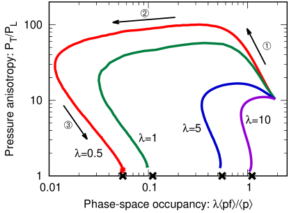
Figure 4: Kinetic theory simulation of the non-equilibrium evolution of the pressure anisotropy and phase-space occupancy (see eq. (72) and surrounding text) for a pure Yang-Mills plasma in the original bottom-up scenario [67]. Here $\lambda=4\pi\alpha_{s}N_{c}$ is the coupling, and the black crosses indicate equilibrium value. The three arrows and associated circled numbers indicate the three stages of bottom-up.

To analyze the first over-occupied stage in the expanding case we examine the Boltzmann equation with an elastic scattering

$$\left(\frac{\partial}{\partial\tau}-\frac{p_{z}}{\tau}\frac{\partial}{\partial p_{z}}\right)f(\tau,p_{z},{\bm{p}}_{\perp})=\frac{\hat{q}}{4}\,\frac{\partial^{2}f}{\partial p_{z}^{2}}\,.$$ (73)

Here the free streaming term on the l.h.s. stems from the expansion of the system, and makes the momentum distribution increasingly anisotropic [68]. On the r.h.s. is the Fokker-Planck operator discussed in Sect. 3, but here we have kept only the most relevant term which competes with the expansion and broadens the momentum distribution. Eq. (73) admits a scaling solution of the form

$$f(\tau,p_{z},p_{T})=\frac{1}{\alpha(Q_{s}\tau)^{2/3}}f_{S}\left(\frac{p_{T}}{Q_{s}},\frac{p_{z}(Q_{s}\tau)^{1/3}}{Q_{s}}\right)\,,$$ (74)

provided one uses the by now familiar estimate for $\hat{q}$ dominated by the hard modes, $\hat{q}\sim\alpha^{2}\int_{\bm{p}}f_{\bm{p}}(1+f_{\bm{p}})$. This scaling solution, which features a decreasing occupancy and an increasing anisotropy, is clearly seen in the numerical simulations of [67] at least for the smallest couplings.

The first over-occupied stage of the bottom up scenario has also been addressed in detail within classical-statistical simulations [48, 28, 54]. It was found that the phase space distribution in the classical simulations reaches the universal scaling form of eq. (74), reflecting the NTFP discussed in Sect. 4.1. In these simulations the effects of plasma instabilities are clearly observed at early times during the approach to the NTFP attractor, but do not appear to significantly affect the longitudinal momentum broadening in the scaling regime, such that $\langle p_{z}^{2}\rangle\sim Q_{s}^{2}(Q_{s}\tau)^{-2/3}$ decreases at late times as in the original bottom scenario. It remains an open question why plasma instabilities do not seem to play a more important role during the first phase of bottom up.

From the scaling solution in eq. (74), we see that the first phase ends at a time $Q_{s}\tau\sim\alpha_{s}^{-3/2}$, and after this point the system in is an under-occupied non-equilibrium state. The estimates and physics for the thermalization of such states described in Sect. 4.2 can be adapted to the expanding case by recognizing that hard modes are essentially free streaming, and thus the energy and number densities of these modes are continually decreasing, so that the energy and number per rapidity ($\tau e$ and $\tau n$ respectively) remains fixed:

$$\tau e_{\rm hard}(\tau)= \frac{Q_{s}^{3}}{\alpha_{s}}\,,$$ (75)

$$\tau n_{\rm hard}(\tau)= \frac{Q_{s}^{2}}{\alpha_{s}}\,.$$ (76)

Using the estimate

$$\hat{q}(\tau)\sim\alpha_{s}^{2}\int_{{\bm{p}}}f_{\bm{p}}(1+f_{{\bm{p}}})\sim\alpha_{s}^{2}\,n_{{\scriptscriptstyle\textrm{hard}}}(\tau)\,,$$ (77)

one finds that because of the expansion the soft scale $p_{\rm soft}(\tau)$ remains constant in time

$$p_{\textrm{soft}}^{2}(\tau)\sim\hat{q}(\tau)\tau\sim\alpha_{s}Q_{s}^{2}\,,$$ (78)

as opposed to increasing as it does in the non-expanding case. Thus, the pressure anisotropy in the second phase is constant and large as seen in Fig. 4. Eq. (58) for the energy density produced by direction radiation by the bath into the soft modes remains valid

$$e_{\rm soft}(\tau)\sim\alpha_{s}\tau e_{\rm hard}(\tau)\sqrt{\frac{\hat{q}(\tau)}{Q_{s}}}\sqrt{\frac{p_{\textrm{soft}}(\tau)}{Q_{s}}}\;,$$ (58)

but now $e_{\rm hard}(\tau)$ and $\hat{q}(\tau)$ are functions of time. Qualitatively, Eq. 58 will hold even if plasma instabilities are present, but $\hat{q}$ will deviate from the estimate in eq. (77), which is based upon elastic scattering by the hard modes. However, because the plasma instabilities are bounded they will not radically change the picture. The second phase of bottom-up ends when $e_{\rm soft}(\tau)\sim p_{\textrm{soft}}^{4}(\tau)$ and the soft bath has thermalized. Equating these two expression one finds that the second phase ends at a time of order $Q_{s}\tau\sim\alpha_{s}^{-5/2}$.

Finally, we analyze the last phase of bottom-up. Here again the physics is identical to the inverse energy cascade discussed in detail in Sect. 4.2.2 for the static system. Eq. (61) for the splitting (or stopping) momentum $p_{\rm split}(\tau)=\alpha_{s}^{2}\hat{q}(\tau)\tau^{2}$, and eq. (64) for $e_{\rm soft}(\tau)$ are unchanged

$$e_{\rm soft}(\tau)\sim e_{\rm hard}(\tau)~{}\frac{p_{\rm split}(\tau)}{Q_{s}}\,,$$ (64)

provided the free streaming result for $e_{\rm hard}(\tau)$ is used. Again, plasma instabilities may modify our estimate for $\hat{q}(\tau)$, but this will not change the overall picture. The system is completely thermalized when $e_{\rm soft}(\tau)$ becomes comparable to $e_{\rm hard}(\tau)$, $\tau e_{\rm soft}(\tau)\sim\tau e_{\rm hard}(\tau)\sim Q_{s}^{3}/\alpha$. Using the fact that $\hat{q}$ is determined by $e_{\rm soft}$ in equilibrium, $\hat{q}(\tau)\sim\alpha_{s}^{2}\,e^{3/4}_{\rm soft}(\tau)$, one readily establishes that the system thermalizes at

$$Q_{s}\tau\sim\alpha_{s}^{-13/5}\,.$$ (79)

We hope that it is evident that the overall picture of bottom-up is quite robust. Ultimately this picture follows from a hard scale $Q_{s}$, kinematics, and generic features of collinear radiation. These features tend to fill up a soft sector first, which then causes a cascade of the energy of the system to the IR. Indeed, an extensive analysis of thermalization when plasma instabilities are present finds many of the same qualitative features of bottom-up with somewhat modified exponents [63].

5 Simulations of early time dynamics and heavy-ion phenomenology

5.1 Approach to hydrodynamics

We now turn to simulations of the early time dynamics and the approach to equilibrium in high-energy heavy ion collisions. Here we will focus on the eventual approach towards local thermal equilibrium, and determine when the evolution can be described with relativistic viscous fluid dynamics.

Viscous fluid dynamics describes the macroscopic evolution of the energy-momentum tensor $T^{\mu\nu}$, based on an expansion around local thermal equilibrium which is controlled by the Knudsen number ${\rm Kn}_{\theta}\sim\tau_{\rm micro}/{\mathcal{T}}_{\rm macro}$, and the proximity to the equilibrium state, which can be quantified by the non-equilibrium corrections to the stress tensor, $T^{\mu\nu}_{\rm non-eq}/T^{\mu\nu}_{\rm eq}$. At early times $\tau\sim 1/Q_{s}$ the longitudinal pressure is much smaller than the transverse pressure $P_{L}\ll P_{T}$ and hydrodynamics does not apply. Consequently, the key question is to understand how $T^{\mu\nu}$ then evolves towards local thermal equilibrium where the longitudinal and transverse pressures are equal $P_{L}=P_{T}$.

Neglecting potential problems related to plasma instabilities, the non-equilibrium evolution of macroscopic quantities such as $T^{\mu\nu}$ can be calculated based on numerical simulations of the effective kinetic theory. Numerical simulation based on QCD kinetic theory were pioneered in [69, 70]; the first complete leading order study for a homogeneous purely gluonic plasma was performed in [67] and subsequently extended to inhomogeneous plasmas [71, 30, 72] as well as homogeneous plasmas of quarks and gluons [73, 74]. Kinetic theory simulations shown in Fig. 5(a) indicate that for realistic coupling strength $\alpha_{s}\gtrsim 0.1$, the evolution of the energy-momentum tensor towards equilibrium is to a good approximation controlled by a single time scale $\tau^{\rm eq}_{R}$, corresponding to the equilibrium relaxation rate

$$\tau_{R}^{\rm eq}(\tau)=\frac{4\pi\eta/s}{T_{\rm Id}(\tau)}\;,$$ (80)

where $\eta/s\propto\lambda^{2}$ is the shear-viscosity to entropy density ratio, and $T_{\rm Id}(\tau)=\propto\tau^{-1/3}$ denotes the temperature of the late-time equilibrium system. Even though an extrapolation to sizeable coupling strength is required to make contact with heavy-ion phenomenology, the dependence on $\alpha_{s}$ is surprisingly weak once $\tau$ is measured in units of $\tau^{\rm eq}_{R}$. When comparing the results for the non-equilibrium evolution of the energy-momentum tensor $T^{\mu\nu}$ in kinetic theory with the asymptotic behavior in viscous hydrodynamics, one concludes that a fluid dynamic description becomes applicable on time scales $\tau_{\text{hydro}}\approx\tau^{\rm eq}_{R}(\tau)$. For phenomenological purposes the coupling constant $\lambda$ can be traded for $\eta/s\propto\lambda^{2}$ yielding the following estimate

$$\tau_{\text{hydro}}\approx 1.1\,{\rm fm}\,\left(\frac{4\pi(\eta/s)}{2}\right)^{{3}/{2}}\left(\frac{\langle\tau s\rangle}{4.1\,{\rm GeV}^{2}}\right)^{-1/2}\left(\frac{\nu_{\text{eff}}}{40}\right)^{1/2},$$ (81)

where $\langle\tau s\rangle$ denotes the entropy density per unity rapidity. $\tau s$ is directly related to the charged particle multiplicity $dN_{\rm ch}/d\eta$, and thereby constrained to be approximately $\approx 4.1\,{\rm GeV}^{2}$ for central Pb+Pb collisions at LHC energies [71]. Since the discussion so far ignores the effects of spatial gradients, both in transverse space and longitudinal rapidity, the estimate in (81) should be understood as a lower bound.

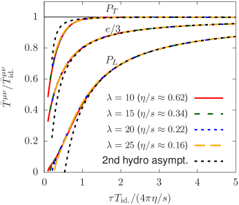
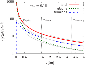
Figure 5: (left) Non-equilibrium evolution of the different components of the average energy-momentum tensor $T^{\mu\nu}={\rm diag}(e,P_{T},P_{T},P_{L})$ compared to viscous fluid dynamics [30, 72]. (right) Evolution of the overall energy density $e$ and the energy density carried by quarks and gluons $e_{g/q}$ [73].

Interestingly one finds that viscous hydrodynamics starts to describe the evolution of the energy-momentum tensor in a regime where both the Knudsen number ${\rm Kn}_{\theta}\approx\tau_{R}^{\rm eq}/\tau$ and the proximity to equilibrium as measured by $1-P_{L}/P_{T}$ are of order unity, indicating that the system is still significantly out-of-equilibrium. Even though this behavior appears to be quite surprising, it is by no means unique to a weakly coupled non-equilibrium description, and similar observations have been reported much earlier in the context of strongly coupled gauge theories [75]. It has become common to distinguish the time when hydrodynamics becomes applicable $\tau_{\text{hydro}}$ (the so called “hydrodynamization” time) from the time $\tau_{\rm eq}$ when the pressure anisotropy is small. Due to the rapid longitudinal expansion, the actual approach towards local pressure isotropy occurs only on much larger time scales $\tau_{\rm eq}\gg\tau_{\text{hydro}}$. Hence the great success of hydrodynamic descriptions of the QGP does not appear to derive from the fact that the system is particularly close to equilibrium throughout most of its space-time evolution, but is rather due to fact that the range of applicability of viscous relativistic fluid appears to be larger than originally anticipated. Notably, these observations have triggered a large number of theoretical studies to further investigate and possibly extend the range of applicability of viscous fluid dynamics [76, 77, 78]. However, a detailed discussion of these topics is beyond the scope of this review.

5.2 Quark production and chemical equilibration

So far most theoretical studies of the early non-equilibrium dynamics have focused on the kinetic equilibration of gluons, while neglecting dynamical fermions in the analysis. However, on a conceptual level it is equally important to understand the transition from an initial state, which is believed to be highly gluon dominated, towards chemical equilibrium where a significant fraction of the energy density is carried by quark degrees of freedom. We note from a phenomenological point of view the chemical composition of the plasma at early times, may have also have interesting consequences, e.g. relating to the questions concerning the chemical equilibration of strange quarks and heavy flavors or the electro-magnetic response of the QGP at very early times after the collision. Even though a complete picture of chemical equilibration along the lines of our discussion in Sec. 4.2 is yet to be established, interesting first results have been reported in the literature. We briefly discuss these results below.

Classical-statistical simulations of quark production at very early times have been pioneered in [79] demonstrating that at realistic coupling strength a significant number of quark anti-quark pairs can be produced in the initial (semi-) hard scattering and in the presence of the strong color fields at very early times. Subsequent studies have refined the lattice approach [80, 81] and further elaborated on quark production in over-occupied systems [82]. However, as classical-statistical simulations involving dynamical fermions are significantly more complicated, studies are yet to reach the same level of sophistication of analogous pure gauge theory simulations.

Quark production during the final radiative break-up stage of the bottom up scenario, has been investigated in the context of jet quenching [59], where it was pointed out that the turbulent nature of the inverse energy cascade ultimately determines the quark/gluon ratio from a local balance of the $g\to q\bar{q}$ and $q\to qg$ processes. However, within the inertial range of the cascade $T_{\rm soft}\ll p\ll p_{\rm split}$ the fraction of energy carried by quarks and anti-quarks $e_{\rm q}/e_{\rm g}\simeq 0.07\times 2N_{f}$ (for three colors) is small compared to the equilibrium ratio $e_{\rm q}/e_{\rm g}\simeq 0.3\times 2N_{f}$, indicating that elastic processes, which are operative at the scales of the soft thermal medium also play a pivotal role in the chemical equilibration process.

The first numerical study implementing all relevant leading order processes of bottom up was performed in [73, 74], indicating that as shown in Fig. 5 the approach to viscous fluid dynamic behavior (discussed in Sect. 5.1) occurs before chemical equilibration of the QGP. A complete leading order analysis of the chemical equilibration mechanism (along the lines of Sect. 4.2) has not yet been given, and should explain these first numerical results and provide guidance to phenomenology.

Notably, the inclusion of dynamical quarks also represent an important step towards calculations of pre-equilibrium photon and dilepton production, and in addressing questions related to the chemical/kinetic equilibration of heavy flavors. While first progress in this direction has been reported in [83] by analyzing a subset of leading order processes, a complete leading order study has not been performed to date.

5.3 Small scale fluctuations and pre-flow

So far we have discussed the microscopic dynamics of the local equilibration process, neglecting the effects of spatial gradients on small scales $\sim c\tau_{\rm hydro}$. However, as discussed in Sect. 2 the inclusion of small scale fluctuations $\sim R_{p}$ is a necessary ingredient for a realistic event-by-event description, since such gradients will lead to the development of “pre-flow”, a pre-cursor to the late stage hydrodynamic flow which starts to build up already during the pre-equilibrium phase. The kinetic theory should evolve these fluctuations and smoothly asymptote to hydrodynamics at late times $\tau\sim\tau_{\rm hydro}$.

A recent extension of the bottom up scenario accounts for small scale fluctuations by explicitly including spatially inhomogeneous fluctuations of the phase space density into the kinetic description [30, 72, 71]. By choosing a representative form for the phase-space distribution to model the initial fluctuations of the stress tensor $\delta T^{\mu\nu}(\tau_{0},{\bm{x}}_{0})$ around a local average $\bar{T}^{\mu\nu}_{\bf x}(\tau_{0})$ at a point ${\bf x}$, the pre-equilibrium evolution of the energy-momentum tensor can then be calculated as

$$T^{\mu\nu}(\tau,{\bf x})\simeq\underbrace{\bar{T}^{\mu\nu}_{\bf x}(\tau)}_{\begin{subarray}{c}\text{non-eq. evolution of}\\ \text{(local) avg. background}\end{subarray}}+\underbrace{\int_{\odot}d^{2}{\bf x}_{0}~{}G^{\mu\nu}_{\alpha\beta}(\tau,\tau_{0},{\bf x},{\bf x}_{0})~{}\delta T^{\alpha\beta}(\tau_{0},{\bf x}_{0})}_{\text{non-eq. evolution of local fluctuations of the stress tensor}}\;,$$ (82)

which is shown schematically in Fig. 6. Here $\bar{T}^{\mu\nu}_{\bf x}(\tau)$ describes the pre-equilibrium evolution of the average energy-momentum tensor and is described by Fig. 5, while $G^{\mu\nu}_{\alpha\beta}$ describes the linear response to initial fluctuations in the thermalizing plasma [30]. Since causality restricts the contributions to the fluctuations at ${\bf x}$, one only needs to integrate the response over the causal circle $\odot$ indicated by the circle at $\tau_{0}=\tau_{\scriptscriptstyle{\rm EKT}}$ in Fig. 6. The relevant response functions $\bar{T}^{\mu\nu}(\tau)$ and $G^{\mu\nu}_{\alpha\beta}$, can be calculated once and for all in kinetic theory, and packaged into a useful “pre-flow” computer code which encapsulates the thermalization process [30].

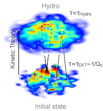
Figure 6: Schematic of the transverse energy density profiles at very early times $(\tau_{0}=\tau_{\scriptscriptstyle{\rm EKT}}\approx 0.1\,{\rm fm}/c)$ and after the first ${\rm fm}/c$ of pre-equilibrium evolution done with kinetic theory $(\tau=\tau_{\text{hydro}})$. At a time $\tau_{\rm hydro}$ the constitutive equations are approximately satisfied (see Fig. 7).

The linear response formalism of eq. (82) can be seen as a systematic extension of earlier studies [84], recognizing universal patterns in the pre-equilibrium evolution of the long wave-length components of the energy-momentum tensor. Short wave-length fluctuations $\ll c\tau_{\rm Hydro}$ are efficiently damped during the pre-equilibrium phase, leading to an effective coarse graining of the spatial profile of the energy-momentum tensor shown schematically in Fig. 6. Then viscous corrections to the energy-momentum tensor are reasonably well approximated by the Navier-Stokes constitutive relations at the time $\tau_{\rm init.}$ when hydrodynamics is initialized. This is shown in Fig. 7 (left), which uses eq. (82) to determine the stress at a time $\tau_{\rm init.}$. Long wave-length fluctuations of the initial energy density determine the pre-flow which develops during thermalization process, and can be reasonably approximated as

$$T^{\tau i}(\tau,{\bf x})\approx-\frac{(\tau-\tau_{0})}{2}\left(\frac{\bar{T}_{\bf x}^{\tau\tau}(\tau)}{\bar{T}_{\bf x}^{\tau\tau}(\tau_{0})}\right)\partial^{i}\bar{T}^{\tau\tau}(\tau_{0},{\bm{x}})\,.$$ (83)

Nevertheless, the results of [30, 72] also demonstrate that a genuine non-equilibrium description is necessary account for the entropy production during the pre-equilibrium phase. Since the subsequent hydrodynamic expansion approximately conserves the overall entropy, this factor two to three increase in entropy during the pre-equilibrium phase is important in relating properties of the initial state to experimentally observed charged particle multiplicities.

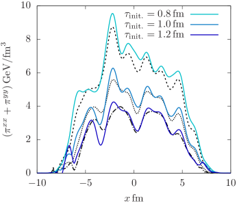
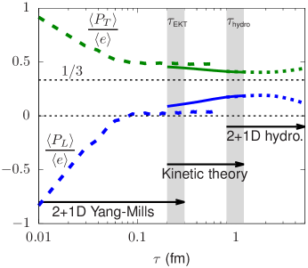
Figure 7: (left) Spatial profiles of the non-equilibrium shear-stress tensor $(\Pi_{xx}+\Pi_{yy})$ (the solid lines) compared to the Navier-Stokes hydrodynamics limit (the dashed lines) after an evolution of $\tau_{\rm init.}$ in the kinetic theory (see eq. (82)). (right) Proof of principle calculation combining different theoretical descriptions to calculate the evolution of energy density $e$,$P_{T}$,$P_{L}$ in a single ${\rm Pb}{+}{\rm Pb}$ event [30, 72].

Finally, by combining the classical-statistical field simulations at early times, the kinetic simulations at intermediate times, and the hydrodynamics simulations at late times, a consistent space-time description of the energy-momentum tensor can be obtained on an event-by-event basis. This is illustrated in Fig. 7 (right) which shows the evolution of longitudinal and transverse pressures in a single ${\rm Pb}{+}{\rm Pb}$ event. In this simulation the first stage up to $\tau_{\rm EKT}$ is treated in the classical IP-Glasma model (see Sect. 2); the second stage up to $\tau_{\rm hydro}$ is treated with QCD kinetics following the outlines of bottom-up; and the final phase is treated with hydrodynamics. The different theoretical descriptions overlap providing a complete picture of the event.

6 Outlook and small systems

We have reviewed the weak coupling description of the thermalization process of the QGP during the first fm/c of high-energy heavy-ion collisions, by dividing the out-of-equilibrium dynamics of non-abelian gauge theories into two broad classes – an over-occupied limit discussed in Sect. 4.1, and an under-occupied limit discussed in Sect. 4.2. Strikingly, the thermalization process in each of these limits exhibits generic scaling features which one would like to observe experimentally.

Indeed, much of the current interest in the equilibration process is driven by exciting new data on the small systems created in proton-proton ($p{+}p$) and proton-nucleus ($p{+}A$) collisions, which show evidence for a transition towards a hydrodynamic regime in nucleus-nucleus $A{+}A$ collisions. A more complete review of the experimental data is given in the literature [85, 2]. In the larger $A+A$ system, the approach to hydrodynamics has been largely understood and quantified within the bottom-up scenario (see for example eq. (81) of Sect. 5), and the physics of the pre-equilibrium stage has been packaged into a useful “pre-flow” computer code that can be used to simulate heavy ion events (see Sect. 5.3). However, as the system size gets smaller, additional scales, such as the transverse radius $R$, play an increasingly important role and truncate the thermalization process. Nevertheless, one can use the bottom-up framework to estimate when hydrodynamics becomes applicable as a function of the multiplicity produced in the collision [30]. Substituting $\tau s=dS/dy/\pi R^{2}$ in eq. (81) we find

$$\frac{\tau_{\rm hydro}}{\rm R}\simeq\left(\frac{dN_{\rm ch}/dy}{63}\right)^{-1/2}\left(\frac{4\pi\eta/s}{2}\right)^{3/2}\left(\frac{S/N_{\rm ch}}{7}\right)^{-1/2}\left(\frac{\nu_{\rm eff}}{40}\right)^{1/2}\,.$$ (84)

Since we expect the bottom up analysis will be strongly modified for $\tau_{\rm hydro}/R\sim 1$, a charged particle multiplicity of order $dN_{\rm ch}/dy\sim 70$ should demarcate the transition to a fully equilibrated regime. So far a detailed understanding, both parametrically and numerically of the transition regime has not been given, though important first steps have been taken [29, 86, 87]. In small systems there are by now many experimental tools, (such as e.g. the hadron chemistry [73] or the system size dependence of the harmonic flow [88, 89]) which can be used to clarify the kinetics of high energy QCD and to guide theory. Further as emphasized in Sect. 4.2.2, studies of the energy loss of jets, both in small and large systems, can inform the study of thermalization of QCD plasmas. We therefore anticipate that, through a combination of phenomenology, formal theory, experiment, and simulation, the community will analyze the transition from cold QCD to the hot QGP in detail, and, more generally, clarify the out-of-equilibrium behavior of non-abelian gauge theories.

DISCLOSURE STATEMENT

The authors are not aware of any affiliations, memberships, funding, or financial holdings that might be perceived as affecting the objectivity of this review.

References

- [1] Heinz U, Snellings R. Ann. Rev. Nucl. Part. Sci. 63:123 (2013)
- [2] Dusling K, Li W, Schenke B. Int. J. Mod. Phys. E25:1630002 (2016)
- [3] Nagle JL, Zajc WA. Ann. Rev. Nucl. Part. Sci. 68:211 (2018)
- [4] Heller MP. Acta Phys. Polon. B47:2581 (2016)
- [5] Keegan L, et al. JHEP 04:031 (2016)
- [6] Baier R, Mueller AH, Schiff D, Son DT. Phys. Lett. B502:51 (2001)
- [7] Bjorken JD. Phys. Rev. D27:140 (1983)
- [8] Gelis F, Schenke B. Ann. Rev. Nucl. Part. Sci. 66:73 (2016)
- [9] McLerran LD, Venugopalan R. Phys. Rev. D49:2233 (1994)
- [10] Kovner A, McLerran LD, Weigert H. Phys. Rev. D52:3809 (1995)
- [11] Kovner A, McLerran LD, Weigert H. Phys. Rev. D52:6231 (1995)
- [12] Lappi T, McLerran L. Nucl. Phys. A772:200 (2006)
- [13] Mazeliauskas A, Teaney D. Phys. Rev. C91:044902 (2015)
- [14] Iancu E, Venugopalan R. 2003. In In *Hwa, R.C. (ed.) et al.: Quark gluon plasma* 249-3363
- [15] Gelis F, Iancu E, Jalilian-Marian J, Venugopalan R. Ann. Rev. Nucl. Part. Sci. 60:463 (2010)
- [16] Krasnitz A, Venugopalan R. Phys. Rev. Lett. 84:4309 (2000)
- [17] Krasnitz A, Venugopalan R. Phys. Rev. Lett. 86:1717 (2001)
- [18] Epelbaum T, Gelis F. Phys. Rev. D88:085015 (2013)
- [19] Romatschke P, Venugopalan R. Phys. Rev. Lett. 96:062302 (2006)
- [20] Romatschke P, Venugopalan R. Phys. Rev. D74:045011 (2006)
- [21] Berges J, Schlichting S. Phys. Rev. D87:014026 (2013)
- [22] Schenke B, Tribedy P, Venugopalan R. Phys. Rev. Lett. 108:252301 (2012)
- [23] Schenke B, Tribedy P, Venugopalan R. Phys. Rev. C86:034908 (2012)
- [24] Mueller AH, Son DT. Phys. Lett. B582:279 (2004)
- [25] Aarts G, Smit J. Nucl. Phys. B511:451 (1998)
- [26] Jeon S. Phys. Rev. C72:014907 (2005)
- [27] Berges J, Schlichting S, Sexty D. Phys. Rev. D86:074006 (2012)
- [28] Berges J, Boguslavski K, Schlichting S, Venugopalan R. Phys. Rev. D89:074011 (2014)
- [29] Greif M, et al. Phys. Rev. D96:091504 (2017)
- [30] Kurkela A, et al. arXiv:1805.00961 [hep-ph] (2018)
- [31] Arnold PB, Cantrell S, Xiao W. Phys. Rev. D81:045017 (2010)
- [32] Blaizot JP, Iancu E, Mehtar-Tani Y. Phys. Rev. Lett. 111:052001 (2013)
- [33] Arnold PB, Moore GD, Yaffe LG. JHEP 01:030 (2003)
- [34] Arnold PB, Moore GD, Yaffe LG. JHEP 05:051 (2003)
- [35] Ghiglieri J, Moore GD, Teaney D. JHEP 03:179 (2018)
- [36] Kurkela A, Moore GD. JHEP 12:044 (2011)
- [37] Blaizot JP, Iancu E. Phys. Rept. 359:355 (2002)
- [38] Landau LD, Lifshits EM. vol. 5 of Course of theoretical physics. London, Pergamon Press; Reading, Mass., Addison-Wesley Pub. Co. (1958)
- [39] Ghiglieri J, Teaney D. Int. J. Mod. Phys. E24:1530013 (2015)
- [40] Ghiglieri J, Moore GD, Teaney D. JHEP 03:095 (2016)
- [41] Arnold PB. Phys. Rev. D79:065025 (2009)
- [42] Arnold PB, Xiao W. Phys. Rev. D78:125008 (2008)
- [43] Baier R, et al. Nucl. Phys. B483:291 (1997)
- [44] Zakharov BG. JETP Lett. 65:615 (1997)
- [45] Gunion JF, Bertsch G. Phys. Rev. D25:746 (1982)
- [46] Arnold PB, Dogan C. Phys. Rev. D78:065008 (2008)
- [47] Blaizot JP, et al. Nucl. Phys. A873:68 (2012)
- [48] Berges J, Boguslavski K, Schlichting S, Venugopalan R. Phys. Rev. D89:114007 (2014)
- [49] Kurkela A, Lu E. Phys. Rev. Lett. 113:182301 (2014)
- [50] Nazarenko S. Lecture Notes in Physics. Springer Berlin Heidelberg (2011)
- [51] Kurkela A, Moore GD. Phys. Rev. D86:056008 (2012)
- [52] Schlichting S. Phys. Rev. D86:065008 (2012)
- [53] Abraao York MC, Kurkela A, Lu E, Moore GD. Phys. Rev. D89:074036 (2014)
- [54] Berges J, Mace M, Schlichting S. Phys. Rev. Lett. 118:192005 (2017)
- [55] Mace M, Schlichting S, Venugopalan R. Phys. Rev. D93:074036 (2016)
- [56] Boguslavski K, Kurkela A, Lappi T, Peuron J. Phys. Rev. D98:014006 (2018)
- [57] Blaizot JP, Mehtar-Tani Y. Annals Phys. 368:148 (2016)
- [58] Zakharov V, L’vov V, Falkovich G. Springer Series in Nonlinear Dynamics. Springer Berlin Heidelberg (2012)
- [59] Mehtar-Tani Y, Schlichting S. JHEP 09:144 (2018)
- [60] Mrowczynski S. Phys. Lett. B314:118 (1993)
- [61] Romatschke P, Strickland M. Phys. Rev. D68:036004 (2003)
- [62] Arnold PB, Lenaghan J, Moore GD. JHEP 08:002 (2003)
- [63] Kurkela A, Moore GD. JHEP 11:120 (2011)
- [64] Bodeker D. JHEP 10:092 (2005)
- [65] Rebhan A, Romatschke P, Strickland M. Phys. Rev. Lett. 94:102303 (2005)
- [66] Arnold PB, Moore GD, Yaffe LG. Phys. Rev. D72:054003 (2005)
- [67] Kurkela A, Zhu Y. Phys. Rev. Lett. 115:182301 (2015)
- [68] Baym G. Phys. Lett. 138B:18 (1984)
- [69] Xu Z, Greiner C. Phys. Rev. C71:064901 (2005)
- [70] El A, Xu Z, Greiner C. Nucl. Phys. A806:287 (2008)
- [71] Keegan L, Kurkela A, Mazeliauskas A, Teaney D. JHEP 08:171 (2016)
- [72] Kurkela A, et al. arXiv:1805.01604 [hep-ph] (2018)
- [73] Kurkela A, Mazeliauskas A arXiv:1811.03040 [hep-ph] (2018)
- [74] Kurkela A, Mazeliauskas A arXiv:1811.03068 [hep-ph] (2018)
- [75] Heller MP, Janik RA, Witaszczyk P. Phys. Rev. Lett. 108:201602 (2012)
- [76] Florkowski W, Heller MP, Spalinski M. Rept. Prog. Phys. 81:046001 (2018)
- [77] Romatschke P. Phys. Rev. Lett. 120:012301 (2018)
- [78] Strickland M, Noronha J, Denicol G. Phys. Rev. D97:036020 (2018)
- [79] Gelis F, Kajantie K, Lappi T. Phys. Rev. Lett. 96:032304 (2006)
- [80] Gelis F, Tanji N. JHEP 02:126 (2016)
- [81] Müller N, Schlichting S, Sharma S. Phys. Rev. Lett. 117:142301 (2016)
- [82] Tanji N, Berges J. Phys. Rev. D97:034013 (2018)
- [83] Berges J, Reygers K, Tanji N, Venugopalan R. Phys. Rev. C95:054904 (2017)
- [84] Vredevoogd J, Pratt S. Phys. Rev. C79:044915 (2009)
- [85] Loizides C. Nucl. Phys. A956:200 (2016)
- [86] Borghini N, Feld S, Kersting N. Eur. Phys. J. C78:832 (2018)
- [87] Kurkela A, Wiedemann UA, Wu B. Phys. Lett. B783:274 (2018)
- [88] Yan L, Ollitrault JY. Phys. Rev. Lett. 112:082301 (2014)
- [89] Mace M, Skokov VV, Tribedy P, Venugopalan R. Phys. Lett. B788:161 (2019)