Sparse hierarchical representation learning on molecular graphs

Abstract.

Architectures for sparse hierarchical representation learning have recently been proposed for graph-structured data, but so far assume the absence of edge features in the graph. We close this gap and propose a method to pool graphs with edge features, inspired by the hierarchical nature of chemistry. In particular, we introduce two types of pooling layers compatible with an edge-feature graph-convolutional architecture and investigate their performance for molecules relevant to drug discovery on a set of two classification and two regression benchmark datasets of MoleculeNet. We find that our models significantly outperform previous benchmarks on three of the datasets and reach state-of-the-art results on the fourth benchmark, with pooling improving performance for three out of four tasks, keeping performance stable on the fourth task, and generally speeding up the training process.

1. Introduction and Related Work

Predicting chemical properties of molecules has become a prominent application of neural networks in recent years. A standard approach in chemistry is to conceptualize groups of individual atoms as functional groups with characteristic properties, and infer the properties of a molecule from a multi-level understanding of the interactions between functional groups. This approach reflects the hierarchical nature of the underlying physics and can be formally understood in terms of renormalization (Lin et al., 2017). It thus seems natural to use machine learning models that learn graph representations of chemical space in a local and hierarchical manner. This can be realized by coarse-graining the molecular graph in a step-wise fashion, with nodes representing effective objects such as functional groups or rings, connected by effective interactions.

Much published work leverages node locality by using graph-convolutional networks with message passing to process local information, see Gilmer et al. (2017) for an overview. In graph classification and regression tasks, usually, only a global pooling step is applied to aggregate node features into a feature vector for the entire graph (Duvenaud et al., 2015; Li et al., 2016; Dai et al., 2016; Gilmer et al., 2017).

An alternative is to aggregate node representations into clusters, which are then represented by a coarser graph (Bruna et al., 2013; Niepert et al., 2016; Defferrard et al., 2016; Monti et al., 2017; Simonovsky and Komodakis, 2017; Fey et al., 2018; Mrowca et al., 2018). Early work uses predefined and fixed cluster assignments during training, obtained by a clustering algorithm applied to the input graph. More recently, dynamic cluster assignments are made on learned node features (Ying et al., 2018; Gao and Ji, 2019; Cangea et al., 2018; Gao et al., 2019). A pioneering step in using learnable parameters to cluster and reduce the graph was the DiffPool layer introduced by Ying et al. (2018). Unfortunately, DiffPool is tied to a disadvantageous quadratic memory complexity that limits the size of graphs and cannot be used for large sparse graphs. A sparse, and therefore more efficient, technique has been proposed by Gao and Ji (2019) and further tested and explored by Cangea et al. (2018); Gao et al. (2019).

Sparse pooling layers have so far not been developed for networks on graphs with both node and edge features. This is particularly important for molecular datasets, where edge features may describe different bond types or distances between atoms. When coarsening the molecular graph, new, effective edges need to be created whose edge features represent the effective interactions between the effective nodes. In this paper we explore two types of sparse hierarchical representation learning methods for molecules that process edge features differently during pooling: a simple pooling layer simply aggregates the features of the involved edges, while a more physically-inspired coarse-graining pooling layer determines the effective edge features using neural networks.

We evaluate our approach on established molecular benchmark datasets (Wu et al., 2018), in particular on the regression datasets ESOL and lipophilicity and the classification datasets BBBP and HIV, on which various models have been benchmarked (Li et al., 2017b; B. Goh et al., 2017a, b; B. Goh et al., 2017c; Goh et al., 2018; Shang et al., 2018; B. Goh et al., 2018; Jaeger et al., 2018; Urban et al., 2018; Feinberg et al., 2018; Zheng et al., 2019; Winter et al., 2019). We obtain significantly better results on the datasets ESOL, lipophilicity, and BBBP, and obtain state-of-the-art results on HIV. Simple pooling layers improve results on BBBP and HIV, while coarse-grain pooling improves results on lipophilicity. In general pooling layers can keep performance at least stable while speeding up training.

2. Approach

2.1. Model architecture

We represent input graphs in a sparse representation using node (${\bm{a}}$) and edge (${\bm{e}}$) feature vectors

(1) $${\bm{a}}^{(0)}_{i} ={\bm{a}}_{i},\enskip i=1,\dots,\;n_{\rm nodes},$$

(2) $${\bm{e}}^{(0)}_{ij} ={\bm{e}}_{ij},\enskip i,j=1,\dots,n_{\rm nodes}\;\mathrm{for}\;j\in\mathrm{NN}(i),$$

where $j$ belongs to the set of nearest-neighbours (NN) of $i$. For chemical graphs we encode the atom type as a one-hot vector and its node degree as an additional entry in ${\bm{a}}_{i}$, while the bond type is one-hot encoded in ${\bm{e}}_{ij}$. Framed in the message-passing framework (Gilmer et al., 2017),the graph-convolutional models we use consist of alternating message-passing steps to process information locally and pooling steps that reduce the graph to a simpler sub-graph. Finally, a read-out phase gathers the node features and computes a feature vector for the whole graph that is fed through a simple perceptron layer in the final prediction step.

Dual-message graph-convolutional layer  Since edge features are an important part of molecular graphs, the model architecture is chosen to give more prominence to edge features. We design a dual-message graph-convolutional layer that supports both node and edge features and treats them similarly. First, we compute an aggregate message ${\bm{m}}^{(k+1)}_{i}$ to a target node from all neighbouring source nodes $j\in{\rm NN}(i)$ using a fully-connected neural network $f_{\bm{W}}$ acting on the source node features ${\bm{a}}^{(k)}_{i}$ and the edge features ${\bm{e}}^{(k)}_{ij}$ of the connecting edge. A self-message ${\bm{s}}^{(k+1)}_{i}={\bm{W}}_{s}^{(k)}\,{\bm{a}}^{(k)}_{i}+{\bm{b}}_{s}^{(k)}$ from the original node features is added to the aggregated result. New node features are computed by applying batch norm (BN) and a ReLU non-linearity, i.e.

(3) $${\bm{m}}^{(k+1)}_{i}=\sum_{j\in\mathrm{N}(i)}f_{{\bm{W}}_{a}}\left({\bm{a}}^{(k)}_{j},{\bm{e}}^{(k)}_{ij}\right)\,,$$

(4) $$\tilde{\bm{a}}^{(k+1)}_{i}=\mathrm{ReLU}\left({\rm BN}\left({\bm{m}}^{(k+1)}_{i}+{\bm{s}}^{(k+1)}_{i}\right)\right)\,.$$

In contrast to the pair-message graph-convolutional layer of Gilmer et al. (2017), we also update the edge feature with the closest node feature vectors via

(5) $${\bm{m}}^{(k+1)}_{ij} =g_{{\bm{W}}_{e}}\left(\tilde{\bm{a}}^{(k+1)}_{i}+\tilde{\bm{a}}^{(k+1)}_{j},{\bm{e}}^{(k)}_{ij}\right),$$

(6) $$\tilde{\bm{e}}^{(k+1)}_{ij} =\mathrm{ReLU}\left(\mathrm{BN}\left({\bm{m}}^{(k+1)}_{ij}+{\bm{s}}^{(k)}_{ij}\right)\right),$$

where $g$ is a fully-connected neural network and ${\bm{s}}^{(k)}_{ij}={\bm{W}}^{(k)}_{e}\,{\bm{e}}^{(k)}_{ij}+{\bm{b}}^{(k)}_{e}$ is the edge feature self-message.

	RMSE results on		ROC-AUC results on
Model	ESOL	Lipophilicity	BBBP	HIV
RF	1.07 $\pm$ 0.19	0.876 $\pm$ 0.040	0.714 $\pm$ 0.000	—
Multitask	1.12 $\pm$ 0.15	0.859 $\pm$ 0.013	0.688 $\pm$ 0.005	0.698 $\pm$ 0.037
XGBoost	0.912 $\pm$ 0.000a	0.799 $\pm$ 0.054	0.696 $\pm$ 0.000	0.756 $\pm$ 0.000
KRR	1.53 $\pm$ 0.06	0.899 $\pm$ 0.043	—	—
GC	0.648 $\pm$ 0.019a	0.655 $\pm$ 0.036	0.690 $\pm$ 0.009	0.763 $\pm$ 0.016
DAG	0.82 $\pm$ 0.08	0.835 $\pm$ 0.039	—	—
Weave	0.553 $\pm$ 0.035a	0.715 $\pm$ 0.035	0.671 $\pm$ 0.014	0.703 $\pm$ 0.039
MPNN	0.58 $\pm$ 0.03	0.719 $\pm$ 0.031	—	—
Logreg	—	—	0.699 $\pm$ 0.002	0.702 $\pm$ 0.018
KernelSVM	—	—	0.729 $\pm$ 0.000	0.792 $\pm$ 0.000
IRV	—	—	0.700 $\pm$ 0.000	0.737 $\pm$ 0.000
Bypass	—	—	0.702 $\pm$ 0.006	0.693 $\pm$ 0.026
Chemception (B. Goh et al., 2017c; Goh et al., 2018)	—	—	—	0.752
Smiles2vec (B. Goh et al., 2017a)	0.63	—	—	0.8
ChemNet (B. Goh et al., 2017b)	—	—	—	0.8
Dummy super node GC (Li et al., 2017b)	—	—	—	0.766
EAGCN (Shang et al., 2018)	—	0.61 $\pm$ 0.02	—	0.83 $\pm$ 0.01
Mol2vec (Jaeger et al., 2018)	0.79	—	—	—
Outer RNN (Urban et al., 2018)	0.62	0.64	—	—
PotentialNet (Feinberg et al., 2018)	0.490 $\pm$ 0.014	—	—	—
SA-BILSTM (Zheng et al., 2019)	—	—	—	0.83 $\pm$ 0.02
RNN encoder (Winter et al., 2019)	0.58	0.62	0.74	—
NoPool	0.410 $\pm$ 0.023	0.551 $\pm$ 0.010	0.846 $\pm$ 0.011	0.825 $\pm$ 0.008
SimplePooling (0.9)	0.410 $\pm$ 0.018	0.536 $\pm$ 0.009	0.839 $\pm$ 0.022	0.824 $\pm$ 0.014
SimplePooling (0.8)	0.417 $\pm$ 0.027	0.542 $\pm$ 0.013	0.869 $\pm$ 0.010	0.816 $\pm$ 0.020
SimplePooling (0.7)	0.485 $\pm$ 0.020	0.563 $\pm$ 0.016	0.859 $\pm$ 0.009	0.825 $\pm$ 0.015
SimplePooling (0.6)	0.413 $\pm$ 0.021	0.622 $\pm$ 0.030	0.852 $\pm$ 0.006	0.840 $\pm$ 0.019
SimplePooling (0.5)	0.437 $\pm$ 0.016	0.637 $\pm$ 0.027	0.851 $\pm$ 0.012	0.822 $\pm$ 0.019
CoarseGrainPooling (0.9)	0.420 $\pm$ 0.015	0.517 $\pm$ 0.005	0.852 $\pm$ 0.010	0.834 $\pm$ 0.015
CoarseGrainPooling (0.8)	0.430 $\pm$ 0.019	0.529 $\pm$ 0.020	0.853 $\pm$ 0.009	0.833 $\pm$ 0.009
CoarseGrainPooling (0.7)	0.472 $\pm$ 0.013	0.530 $\pm$ 0.005	0.856 $\pm$ 0.012	0.830 $\pm$ 0.007
CoarseGrainPooling (0.6)	0.495 $\pm$ 0.053	0.536 $\pm$ 0.026	0.838 $\pm$ 0.020	0.824 $\pm$ 0.026
CoarseGrainPooling (0.5)	0.412 $\pm$ 0.031	0.535 $\pm$ 0.009	0.858 $\pm$ 0.023	0.826 $\pm$ 0.010

Table 1. (Top) Literature results for the MoleculeNet benchmarks comparing RMSE and ROC-AUC results, on a range of models. Benchmarks without reference come from Wu et al. (2018), except those values decorated with ^a, which come from Feinberg et al. (2018). (Bottom) Our model with coarse-grain pooling, simple pooling, and without pooling. The number in brackets specifies the pooling keep ratio $\rho$ of the pooling layer.

Pooling layer  Pooling layers, as introduced in Gao and Ji (2019), reduce the number of nodes by a fraction

(7) $$\rho=K/n^{(k)}_{\rm nodes},$$

specified as a hyperparameter, via scoring all nodes using a learnable projection vector ${\bm{p}}^{(k)}$, and then selecting the $K$ nodes with the highest score $y^{(k)}_{i}$. In order to make the projection vector ${\bm{p}}^{(k)}$ trainable, and thus the node selection differentiable, ${\bm{p}}^{(k)}$ is also used to determine a gating for each feature vector via

(8) $$y^{(k)}_{i}={\bm{p}}^{(k)}\cdot\tilde{\bm{a}}^{(k)}_{i}\,,\qquad{\bm{a}}^{(k)}_{i}=\tilde{\bm{a}}^{(k)}_{i}\tanh\left({y^{(k)}_{i}}\right)\,,$$

where we only keep the top-$K$ nodes and their gated feature vectors ${\bm{a}}^{(k)}_{i}$.

Pooling nodes requires the creation of new, effective edges between kept nodes while keeping the graph sparse. We discuss in Section 2.2 how to solve this problem in the presence of edge features.

Gather layer  After graph-convolutional and pooling layers, a graph gathering layer is required to map from node and edge features to a global feature vector. Assuming that the dual-message message-passing steps are powerful enough to distribute the information contained in the edge features to the adjacent node features, we gather over node features only by concatenating max and sum, and acting with a $\mathrm{tanh}$ non-linearity on the result. All models have an additional linear layer that acts on each node individually before applying the gather layer and a final perceptron layer.

2.2. Pooling with edge features

An important step of the pooling process is to create new edges based on the connectivity of the nodes before pooling in order to keep the graph sufficiently connected. For graphs with edge features this process also has to create new edge features. In addition, the algorithm must be parallel for performance reasons.

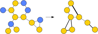
We tackle these issues by specifying how to combine edge features into an effective edge feature between remaining (kept) nodes. If a single dropped node or a pair of dropped nodes connect two kept nodes, we construct a new edge and drop the the ones linked to the dropped nodes. (see Fig. 1).

Figure 1. Schematic of a graph pooling step (yellow nodes are kept, blue nodes are dropped). Dangling nodes are removed, together with their connecting edges. Pairs of edges connecting a dropped node to two kept nodes are coarse-grained to a new edge (heavy lines). New edges can also be constructed between kept nodes connected by two dropped nodes (heaviest line).

We propose two layers to calculate the replacement effective edge feature from the dropped edge features. A simple pooling layer computes an effective edge-feature by summing all edge feature vectors along the paths connecting pairs of kept nodes. When multiple paths between a pair of nodes are simultaneously reduced, this method will generate overlapping effective edge features. We reduce these to a single vector of the sum of overlapping edge feature vectors.

We know however that in chemistry effective interactions are more complex functions of the involved component features. Using this as an inspiration, we propose a more expressive coarse-graining pooling layer, which is obtained by replacing the simple aggregation function with neural networks to compute effective edge features. In particular, we use two fully-connected neural networks. The first network maps the atom and adjoining edge feature vectors of dropped nodes to a single effective-edge feature. The second network calculates effective edge features for kept edges (between kept nodes) to account for an effective coarse-grained interaction compensating for deleted nodes.

We use pooling layers after every convolutional layer except for the final one. For $N$ convolutional layers, the number of nodes thus gets reduced by a factor $\rho^{N-1}$. This compression not only gets rid of irrelevant information but also reduces memory requirements and makes training faster, as we show in the experiments in Sec. 3.

3. Experimental Results on MoleculeNet

Model parameters and implementation  We use hyperparameter tuning with the hyperband algorithm (Li et al., 2018) to decide on the number of stacks and channel dimensions of graph-convolutional and pooling layers while keeping the pooling keep ratio defined in equation 7 fixed. All our models were implemented in PyTorch and trained on a single Nvidia Tesla K80 GPU using the Adam optimizer with a learning rate of $0.0001$.

Evaluation on MoleculeNet  We evaluate our models with and without pooling layers on the MoleculeNet benchmark set (Wu et al., 2018). We focus on four different datasets, comprised of the regression benchmarks ESOL (1128 molecules) and Lipophilicity (4200 molecules), where performance was evaluated by RMSE, and the classification benchmarks on the BBBP (2039 molecules) and HIV (41127 molecules) datasets, evaluated via ROC-AUC. Following Wu et al. (2018), we used a scaffold split for the classification datasets as provided by the DeepChem package. Apart from the benchmarks generated in the original paper, various models have been evaluated on these datasets (Li et al., 2017b; B. Goh et al., 2017a, b; B. Goh et al., 2017c; Goh et al., 2018; Shang et al., 2018; B. Goh et al., 2018; Jaeger et al., 2018; Urban et al., 2018; Feinberg et al., 2018; Zheng et al., 2019; Winter et al., 2019). An overview of the results in the literature can be found in the top of Table 1. Our results are the mean and standard deviation of 5 runs over 5 random splits (ESOL, Lipophilicity) or 5 runs over the same scaffold split (BBBP, HIV). Datasets were split into training (80%), validation (10%), and held-out test sets (10%). The validation set was used to tune model hyperparameters. All reported metrics are results on the test set. The results of our models with and without pooling are displayed in the lower part of the table.

pooling keep ratio	0.9	0.8	0.7	0.6	0.5
Speed-up	16%	24%	47%	55%	70%

Table 2. Speed-up of pooling runs of the HIV data set using Simple Pooling. The speed-up is measured as increase in speed in terms of elapsed real time compared to the run without pooling layer.

For the regression tasks, we found that our models significantly outperformed previous models for both datasets, with pooling layers keeping performance stable for ESOL and the coarse-grain pooling layer significantly improving results for Lipophilicity (see Table 1). Regarding classification tasks, we found that our models significantly outperformed previous models on BBBP and also exceeded previous benchmarks for the HIV dataset. For both datasets simple pooling layers improved performance. Curiously, the extent to which pooling layers improve performance and which layer is better suited for a particular task strongly depends on the dataset. It seems that simple pooling performs much better for classification tasks while for regression tasks it depends on the dataset.

We also measure the speed-up given by pooling layers during the evaluation on the HIV dataset in terms of elapsed real-time, using the simple pooling layer. The results are displayed in Table 2. We see significant speed-ups for moderate values of the pooling ratio.

4. Conclusion

We introduce two graph-pooling layers for sparse graphs with node and edge features and evaluate their performance on molecular graphs. While our model without pooling significantly outperforms benchmarks on ESOL, lipophilicity and BBBP and reaches state-of-the-art results on HIV in the MoleculeNet dataset, we find that our pooling methods improve performance and provide a speedup of up to 70% in the training of graph-convolutional neural networks that utilize edge features, along with a reduction in memory requirements.

While all experiments have been performed on datasets comprised of small, druglike molecules, we expect even stronger performance for datasets comprised of larger graphs like protein structures, where pooling can create a large, sequential hierarchy of graphs. More generally, our work may result in more pertinent and information-effective latent space representations for graph-based machine learning models.

Appendix A Supplementary Material

A.1. Material science application: Clean Energy Project 2017 dataset

pooling	Multi-task			Single-task
ratio	$R^{2}$ on PCE	$R^{2}$ on GAP	$R^{2}$ on HOMO	$R^{2}$ on PCE
none	0.862 $\pm$ 0.005	0.967 $\pm$ 0.001	0.981 $\pm$ 0.000	0.866 $\pm$ 0.003
0.9	0.863 $\pm$ 0.003	0.966 $\pm$ 0.001	0.981 $\pm$ 0.000	0.862 $\pm$ 0.002
0.8	0.860 $\pm$ 0.003	0.966 $\pm$ 0.001	0.981 $\pm$ 0.001	0.859 $\pm$ 0.004
0.7	0.856 $\pm$ 0.003	0.964 $\pm$ 0.001	0.980 $\pm$ 0.001	0.855 $\pm$ 0.004
0.6	0.854 $\pm$ 0.007	0.962 $\pm$ 0.002	0.979 $\pm$ 0.001	0.853 $\pm$ 0.003
0.5	0.844 $\pm$ 0.003	0.955 $\pm$ 0.002	0.974 $\pm$ 0.001	0.833 $\pm$ 0.007
	RMSE on PCE	RMSE on GAP	RMSE on HOMO	RMSE on PCE
none	0.217 $\pm$ 0.004	0.177 $\pm$ 0.002	0.134 $\pm$ 0.001	0.215 $\pm$ 0.002
0.9	0.217 $\pm$ 0.002	0.180 $\pm$ 0.002	0.134 $\pm$ 0.001	0.218 $\pm$ 0.002
0.8	0.220 $\pm$ 0.002	0.179 $\pm$ 0.002	0.135 $\pm$ 0.003	0.220 $\pm$ 0.003
0.7	0.179 $\pm$ 0.097	0.148 $\pm$ 0.080	0.112 $\pm$ 0.060	0.223 $\pm$ 0.003
0.6	0.224 $\pm$ 0.005	0.190 $\pm$ 0.005	0.143 $\pm$ 0.004	0.225 $\pm$ 0.003
0.5	0.232 $\pm$ 0.002	0.208 $\pm$ 0.004	0.159 $\pm$ 0.003	0.239 $\pm$ 0.005

Table 3. Multi-task and single-task benchmark $R^{2}$ results for power conversion efficiency (PCE), band gap (GAP), and highest occupied molecular orbital (HOMO) energy of the CEP-2017 benchmark for different ratios of kept nodes in each pooling step (averaged over 5 runs, with 5 random splits). Speedup of pooling runs is measured in terms of elapsed real time compared to the run without pooling.

In this section, we propose a regression benchmark for hierarchical models using the 2017 non-fullerene electron-acceptor update (Lopez et al., 2017) to the Clean Energy Project molecular library (Hachmann et al., 2011). We refer to this dataset as CEP-2017. This dataset was generated by combining molecular fragments from a reference library generating 51256 unique molecules. These molecular graphs were then used as input to density functional theory electronic-structure calculations of quantum-mechanical observables (such as GAP and HOMO). Restrictions of the crowd-sourced computing platform limited these structures to molecules of 306 electrons or less. The direct observables quantities are then used in a physically motivated but empirical Scharber (Scharber et al., 2006) model to predict power conversion efficiency (PCE). This efficiency is the ultimate figure of merit for a new photovoltaic material.

We emphasize that this data, generated with an approximate density functional theory method, and then used in an empirical PCE model, lacks predictive power in terms of design of new materials. However a machine learning model built on this data is likely to be transferable to other molecular datasets built on higher level theory (such as coupled-cluster calculations) or experimental ground truth. As we are anticipating this future application of the method, we use the raw (_calc) values rather than the Gaussian process regressed (to a small experimental dataset) values (_calib).

The method of construction of the dataset allows us to highlight the coarse-graining interpretation of the pooling layers introduced in the main text, in terms of the explicit combinatorial building blocks of the non-fullerene electron acceptors.

In Table 3, we show multi-task and single-task test set evaluation $R^{2}$ results for the power conversion efficiency (PCE), the band gap (GAP), and the highest occupied molecular orbital (HOMO) energy. We used a dual-message graph-convolutional model with three graph-convolutional layers with node channel dimensions ${[}512,512,512{]}$ and edge channel dimensions ${[}128,128,128{]}$ with two interleaved layers of simple pooling. We found our model to be a powerful predictor of both fundamental quantum-mechanical properties (GAP and HOMO), and to a lesser extend the more empirical PCE figure. The inclusion of pooling layers resulted in a significant speedup and only a very mild decay in performance.

A.2. Pooling layers illustrations

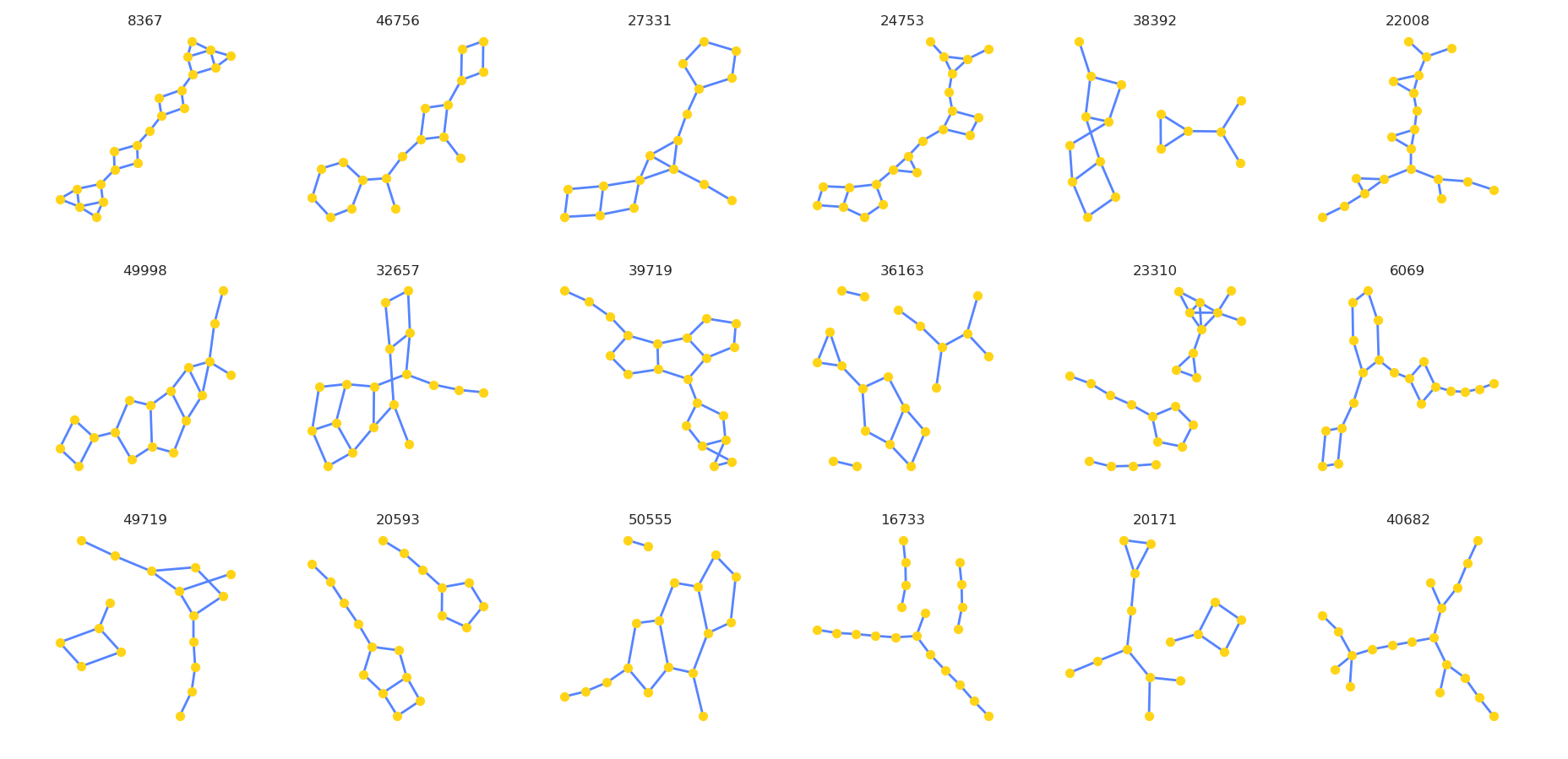
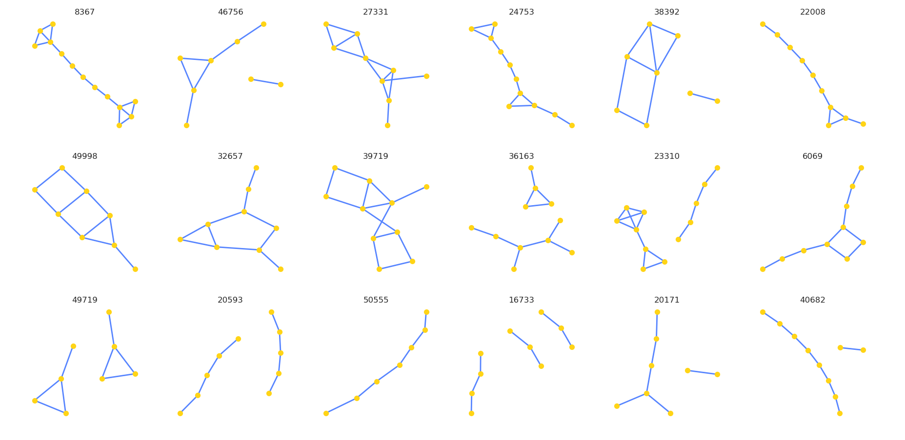
In Fig. 2(a-c) we visualize the effect of two consecutive pooling layers (each keeping only 50% of the nodes) on a batch of molecules for a DM-SimplePooling model trained on a random split of the CEP-2017 dataset introduced in Sec. A.1. After the first pooling layer (Fig. 2(b)), the model has approximately learned to group rings and identify the backbones or main connected chains of the molecules. After the second pooling layer (Fig. 2(c)), the molecular graphs have been reduced to basic, abstract components connected by chains, encoding a coarse-grained representation of the original molecules. Disconnected parts can be interpreted as a consequence of the aggressive pooling forcing the model to pay attention to the parts it considers most relevant for the task at hand.

Molecular graphs before pooling

(a)

Coarse-grained graphs after pooling layer 1.

(b)

Coarse-grained graphs after pooling layer 2.

(c)

Figure 2. Pooling of molecular graphs (heavy atoms only) sampled from CEP-2017 dataset.

Dataset	Model	Keep ratio	Node Channels	Edge Channels
ESOL	NoPooling		[128, 128]	[128, 128]
	CoarseGrainPooling	0.9	[128, 128]	[256, 256]
		0.8	[128, 128]	[64, 64]
		0.7	[512, 512, 512]	[128, 128, 128]
		0.6	[256, 256, 256]	[128, 128, 128]
		0.5	[128, 128]	[64, 64]
	SimplePooling	0.9	[256, 256]	[128, 128]
		0.8	[256, 256, 256]	[256, 256, 256]
		0.7	[128, 128, 128]	[128, 128, 128]
		0.6	[512, 512]	[128, 128]
		0.5	[256, 256]	[256, 256]
Lipophilicity	NoPooling		[256, 256, 256]	[64, 64, 64]
	CoarseGrainPooling	0.9	[256, 256]	[128, 128]
		0.8	[256, 256]	[64, 64]
		0.7	[256, 256]	[64, 64]
		0.6	[256, 256]	[256, 256]
		0.5	[512, 512]	[64, 64]
	SimplePooling	0.9	[512, 512]	[64, 64]
		0.8	[128, 128]	[128, 128]
		0.7	[256, 256]	[128, 128]
		0.6	[512, 512]	[128, 128]
		0.5	[256, 256]	[128, 128]
BBBP	NoPooling		[128, 128]	[256, 256]
	CoarseGrainPooling	0.9	[256, 256]	[256, 256]
		0.8	[512, 512]	[256, 256]
		0.7	[128, 128, 128]	[128, 128, 128]
		0.6	[256, 256]	[64, 64]
		0.5	[256, 256, 256]	[64, 64, 64]
	SimplePooling	0.9	[128, 128, 128]	[256, 256, 256]
		0.8	[512, 512]	[128, 128]
		0.7	[256, 256]	[64, 64]
		0.6	[512, 512]	[256, 256]
		0.5	[128, 128, 128]	[64, 64, 64]
HIV	All models		[512, 512, 512]	[128, 128, 128]

Table 4. Graph-convolutional model hyperparameters used in this work.

References

- (1)
- Altae-Tran et al. (2017) Han Altae-Tran, Bharath Ramsundar, Aneesh S. Pappu, and Vijay S. Pande. 2017. Low Data Drug Discovery with One-shot Learning. American Chemical Society 3 (2017). http://arxiv.org/abs/1611.03199
- B. Goh et al. (2017a) Garrett B. Goh, Nathan O. Hodas, Charles Siegel, and Abhinav Vishnu. 2017a. SMILES2Vec: An Interpretable General-Purpose Deep Neural Network for Predicting Chemical Properties. (12 2017). arXiv:https://arxiv.org/abs/1712.02034 https://arxiv.org/abs/1712.02034
- B. Goh et al. (2018) Garrett B. Goh, Charles Siegel, Abhinav Vishnu, and Nathan Hodas. 2018. Using Rule-Based Labels for Weak Supervised Learning: A ChemNet for Transferable Chemical Property Prediction. 302–310. https://doi.org/10.1145/3219819.3219838
- B. Goh et al. (2017b) Garrett B. Goh, Charles Siegel, Abhinav Vishnu, and Nathan O. Hodas. 2017b. ChemNet: A Transferable and Generalizable Deep Neural Network for Small-Molecule Property Prediction. (12 2017). arXiv:https://arxiv.org/abs/1712.02734 https://arxiv.org/abs/1712.02734
- B. Goh et al. (2017c) Garrett B. Goh, Charles Siegel, Abhinav Vishnu, Nathan O. Hodas, and Nathan Baker. 2017c. Chemception: A Deep Neural Network with Minimal Chemistry Knowledge Matches the Performance of Expert-developed QSARQSPR Models. (06 2017). arXiv:https://arxiv.org/abs/1706.06689 https://arxiv.org/abs/1706.06689
- Bruna et al. (2013) Joan Bruna, Wojciech Zaremba, Arthur Szlam, and Yann LeCun. 2013. Spectral Networks and Locally Connected Networks on Graphs. preprint (2013). arXiv:1312.6203 http://arxiv.org/abs/1312.6203
- Cangea et al. (2018) Cătălina Cangea, Petar Veličković, Nikola Jovanović, Thomas Kipf, and Pietro Liò. 2018. Towards Sparse Hierarchical Graph Classifiers. Workshop on Relational Representation Learning (R2L) at NIPS (2018). arXiv:1811.01287 http://arxiv.org/abs/1811.01287
- Dai et al. (2016) Hanjun Dai, Bo Dai, and Le Song. 2016. Discriminative Embeddings of Latent Variable Models for Structured Data. Proceedings of the International Conference on Machine Learning (ICML) 48 (2016). arXiv:1603.05629 http://arxiv.org/abs/1603.05629
- Defferrard et al. (2016) Michaël Defferrard, Xavier Bresson, and Pierre Vandergheynst. 2016. Convolutional Neural Networks on Graphs with Fast Localized Spectral Filtering. Advances in Neural Information Processing Systems (NIPS) 29 (2016). arXiv:1606.09375 http://arxiv.org/abs/1606.09375
- Duvenaud et al. (2015) David K Duvenaud, Dougal Maclaurin, Jorge Iparraguirre, Rafael Bombarell, Timothy Hirzel, Alán Aspuru-Guzik, and Ryan P Adams. 2015. Convolutional Networks on Graphs for Learning Molecular Fingerprints. In Advances in Neural Information Processing Systems 28, C. Cortes, N. D. Lawrence, D. D. Lee, M. Sugiyama, and R. Garnett (Eds.). Curran Associates, Inc., 2224–2232. https://arxiv.org/abs/1509.09292
- Feinberg et al. (2018) Evan N. Feinberg, Debnil Sur, Zhenqin Wu, Brooke E. Husic, Huanghao Mai, Yang Li, Saisai Sun, Jianyi Yang, Bharath Ramsundar, and Vijay S. Pande. 2018. PotentialNet for Molecular Property Prediction. ACS Central Science 4, 11 (2018), 1520–1530. https://doi.org/10.1021/acscentsci.8b00507 arXiv:https://doi.org/10.1021/acscentsci.8b00507
- Fey et al. (2018) Matthias Fey, Jan Eric Lenssen, Frank Weichert, and Heinrich Müller. 2018. SplineCNN: Fast Geometric Deep Learning with Continuous B-Spline Kernels. IEEE/CVF Conference on Computer Vision and Pattern Recognition (CVPR) (2018). arXiv:1711.08920 http://arxiv.org/abs/1711.08920
- Gao et al. (2019) Hongyang Gao, Yongjun Chen, and Shuiwang Ji. 2019. Learning Graph Pooling and Hybrid Convolutional Operations for Text Representations. preprint abs/1901.06965 (2019). arXiv:1901.06965 http://arxiv.org/abs/1901.06965
- Gao and Ji (2019) Hongyang Gao and Shuiwang Ji. 2019. Graph U-Net. ICLR 2019 Conference Blind Submission (2019). https://openreview.net/forum?id=HJePRoAct7
- Gilmer et al. (2017) Justin Gilmer, Samuel S. Schoenholz, Patrick F. Riley, Oriol Vinyals, and George E. Dahl. 2017. Neural Message Passing for Quantum Chemistry, In ICML. arxiv:1704.01212. http://arxiv.org/abs/1704.01212v2
- Goh et al. (2018) G.B. Goh, C. Siegel, A. Vishnu, N. Hodas, and N. Baker. 2018. How Much Chemistry Does a Deep Neural Network Need to Know to Make Accurate Predictions?. In 2018 IEEE Winter Conference on Applications of Computer Vision (WACV). 1340–1349. https://doi.org/10.1109/WACV.2018.00151
- Hachmann et al. (2011) Johannes Hachmann, Roberto Olivares-Amaya, Sule Atahan-Evrenk, Carlos Amador-Bedolla, Roel S. Sánchez-Carrera, Aryeh Gold-Parker, Leslie Vogt, Anna M. Brockway, and Alán Aspuru-Guzik. 2011. The Harvard Clean Energy Project: Large-Scale Computational Screening and Design of Organic Photovoltaics on the World Community Grid. The Journal of Physical Chemistry Letters 2, 17 (aug 2011), 2241–2251. https://doi.org/10.1021/jz200866s
- Jaeger et al. (2018) Sabrina Jaeger, Simone Fulle, and Samo Turk. 2018. Mol2vec: Unsupervised Machine Learning Approach with Chemical Intuition. Journal of Chemical Information and Modeling 58, 1 (2018), 27–35. https://doi.org/10.1021/acs.jcim.7b00616 arXiv:https://doi.org/10.1021/acs.jcim.7b00616 PMID: 29268609.
- Li et al. (2017a) Junying Li, Deng Cai, and Xiaofei He. 2017a. Learning Graph-Level Representation for Drug Discovery. (2017). arXiv:1709.03741 http://arxiv.org/abs/1709.03741
- Li et al. (2017b) Junying Li, Deng Cai, and Xiaofei He. 2017b. Learning Graph-Level Representation for Drug Discovery. CoRR abs/1709.03741 (2017). arXiv:1709.03741 http://arxiv.org/abs/1709.03741
- Li et al. (2018) Lisha Li, Kevin Jamieson, Giulia DeSalvo, Afshin Rostamizadeh, and Ameet Talwalkar. 2018. Hyperband: A Novel Bandit-Based Approach to Hyperparameter Optimization. Journal of Machine Learning Research 18, 185 (2018), 1–52. http://jmlr.org/papers/v18/16-558.html
- Li et al. (2016) Yujia Li, Daniel Tarlow, Marc Brockschmidt, and Richard S. Zemel. 2016. Gated Graph Sequence Neural Networks. International Conference on Learning Representations (ICLR) (2016). arXiv:1511.05493 http://arxiv.org/abs/1511.05493
- Lin et al. (2017) Henry W. Lin, Max Tegmark, and David Rolnick. 2017. Why Does Deep and Cheap Learning Work So Well? Journal of Statistical Physics 168, 6 (jul 2017), 1223–1247. https://doi.org/10.1007/s10955-017-1836-5
- Lopez et al. (2017) Steven A. Lopez, Benjamin Sanchez-Lengeling, Julio de Goes Soares, and Alán Aspuru-Guzik. 2017. Design Principles and Top Non-Fullerene Acceptor Candidates for Organic Photovoltaics. Joule 1, 4 (dec 2017), 857–870. https://doi.org/10.1016/j.joule.2017.10.006
- Monti et al. (2017) Federico Monti, Davide Boscaini, Jonathan Masci, Emanuele Rodolà, Jan Svoboda, and Michael M. Bronstein. 2017. Geometric deep learning on graphs and manifolds using mixture model CNNs. IEEE Conference on Computer Vision and Pattern Recognition (CVPR) (2017). arXiv:1611.08402 http://arxiv.org/abs/1611.08402
- Mrowca et al. (2018) Damian Mrowca, Chengxu Zhuang, Elias Wang, Nick Haber, Li Fei-Fei, Joshua B. Tenenbaum, and Daniel L. K. Yamins. 2018. Flexible Neural Representation for Physics Prediction. Advances in Neural Information Processing Systems (NIPS) 31 (2018). arXiv:1806.08047 http://arxiv.org/abs/1806.08047
- Niepert et al. (2016) Mathias Niepert, Mohamed Ahmed, and Konstantin Kutzkov. 2016. Learning Convolutional Neural Networks for Graphs. Proceedings of the International Conference on Machine Learning (ICML) 48 (2016). arXiv:1605.05273 http://arxiv.org/abs/1605.05273
- Scharber et al. (2006) M. C. Scharber, D. Mühlbacher, M. Koppe, P. Denk, C. Waldauf, A. J. Heeger, and C. J. Brabec. 2006. Design Rules for Donors in Bulk-Heterojunction Solar Cells—Towards 10 % Energy-Conversion Efficiency. Advanced Materials 18, 6 (mar 2006), 789–794. https://doi.org/10.1002/adma.200501717
- Shang et al. (2018) Chao Shang, Qinqing Liu, Ko-Shin Chen, Jiangwen Sun, Jin Lu, Jinfeng Yi, and Jinbo Bi. 2018. Edge Attention-based Multi-Relational Graph Convolutional Networks. arXiv e-prints, Article arXiv:1802.04944 (Feb 2018), arXiv:1802.04944 pages. arXiv:stat.ML/1802.04944 https://arxiv.org/pdf/1802.04944v1.pdf
- Simonovsky and Komodakis (2017) Martin Simonovsky and Nikos Komodakis. 2017. Dynamic Edge-Conditioned Filters in Convolutional Neural Networks on Graphs. 2017 IEEE Conference on Computer Vision and Pattern Recognition (CVPR) (2017), 29–38. http://arxiv.org/abs/1704.02901v3
- Urban et al. (2018) Gregor Urban, Niranjan Subrahmanya, and Pierre Baldi. 2018. Inner and Outer Recursive Neural Networks for Chemoinformatics Applications. Journal of Chemical Information and Modeling 58, 2 (2018), 207–211. https://doi.org/10.1021/acs.jcim.7b00384 arXiv:https://doi.org/10.1021/acs.jcim.7b00384 PMID: 29320180.
- Winter et al. (2019) Robin Winter, Floriane Montanari, Frank Noé, and Djork-Arné Clevert. 2019. Learning continuous and data-driven molecular descriptors by translating equivalent chemical representations. Chem. Sci. 10 (2019), 1692–1701. Issue 6. https://doi.org/10.1039/C8SC04175J
- Wu et al. (2018) Zhenqin Wu, Bharath Ramsundar, Evan N. Feinberg, Joseph Gomes, Caleb Geniesse, Aneesh S. Pappu, Karl Leswing, and Vijay S. Pande. 2018. MoleculeNet: A Benchmark for Molecular Machine Learning. Chemical Science 2 (2018). arXiv:1703.00564 http://arxiv.org/abs/1703.00564
- Ying et al. (2018) Rex Ying, Jiaxuan You, Christopher Morris, Xiang Ren, William L. Hamilton, and Jure Leskovec. 2018. Hierarchical Graph Representation Learning with Differentiable Pooling. Advances in Neural Information Processing Systems (NIPS) 31 (2018). arXiv:1806.08804 http://arxiv.org/abs/1806.08804
- Zheng et al. (2019) Shuangjia Zheng, Xin Yan, Yuedong Yang, and Jun Xu. 2019. Identifying Structure–Property Relationships through SMILES Syntax Analysis with Self-Attention Mechanism. Journal of Chemical Information and Modeling 59, 2 (2019), 914–923. https://doi.org/10.1021/acs.jcim.8b00803 arXiv:https://doi.org/10.1021/acs.jcim.8b00803 PMID: 30669836.