Gaia DR2 distances to Collinder 419 and NGC 2264 and new astrometric orbits for HD 193 322 Aa,Ab and 15 Mon Aa,Ab

Abstract

Context. On the one hand, the second data release of the Gaia mission (Gaia DR2) has opened a trove of astrometric and photometric data for Galactic clusters within a few kpc of the Sun. On the other hand, lucky imaging has been an operational technique to measure the relative positions of visual binary systems for a decade and a half, a time sufficient to apply its results to the calculation of orbits of some massive multiple systems within $\sim$1 kpc of the Sun.

Aims. As part of an ambitious research program to measure distances to Galactic stellar groups (including clusters) containing O stars, I start with two of the nearest examples: Collinder 419 in Cygnus and NGC 2264 in Monoceros. The main ionizing source for both clusters is a multiple system with an O-type primary: HD 193 322 and 15 Mon, respectively. For each of those two multiple systems I aim to derive new astrometric orbits for the Aa,Ab components.

Methods. First, I present a method that uses Gaia DR2 $G$+$G_{\rm BP}$+$G_{\rm RP}$ photometry, positions, proper motions, and parallaxes to obtain the membership and distance of a stellar group and apply it to Collinder 419 and NGC 2264. Second, I present a new code that calculates astrometric orbits by searching the whole seven-parameter orbit space and apply it to HD 193 322 Aa,Ab and 15 Mon Aa,Ab using as input literature data from the Washington Double Star Catalog (WDS) and the AstraLux measurements recently presented by Maíz Apellániz et al. (2019).

Results. I obtain Gaia DR2 distances of $1006^{+37}_{-34}$ pc for Collinder 419 and $719\pm 16$ pc for NGC 2264, with the main contribution to the uncertainties coming from the spatial covariance of the parallaxes. The two NGC 2264 subclusters are at the same distance (within the uncertainties) and they show a significant relative proper motion. The distances are shown to be robust. HD 193 322 Aa,Ab follows an eccentric ($e=0.58^{+0.03}_{-0.04}$) orbit with a period of $44\pm 1$ a and the three stars it contains have a total mass of $76.1^{+9.9}_{-7.4}$ M_⊙. The orbit of 15 Mon Aa,Ab is even more eccentric ($e=0.770^{+0.023}_{-0.030}$), with a period of $108\pm 12$ a and a total mass of $45.1^{+3.6}_{-3.3}$ M_⊙ for its two stars.

1 Introduction

 The second data release (DR2) of the Gaia mission (Prusti et al., 2016) took place in April 2018 (Brown et al., 2018). Gaia DR2 includes optical photometry for over $1.3\cdot 10^{9}$ sources in the three bands $G$, $G_{\rm BP}$, and $G_{\rm RP}$ and five-parameter astrometry (positions, parallaxes, and proper motions) for a similar number of sources. Gaia DR2 constitutes the largest ever collection of such precise photometry and astrometry. The data is not only precise but also accurate, as several studies have confirmed with respect to the astrometry and photometry (e.g. Arenou et al. 2018; Evans et al. 2018; Lindegren et al. 2018a; Luri et al. 2018; Maíz Apellániz & Weiler 2018, note that this list is incomplete as Gaia DR2 calibration is an ongoing effort). Nevertheless, to achieve the highest accuracy one needs to read the “fine print” of the papers above, as there are biases and quality issues lurking in the data. The Gaia team maintains a “known issues” web page that should be consulted before using the data (details are given in the next section).

Gaia represents a giant leap for astrometry but, of course, it has limitations. One is its inability to separate close binaries, as few pairs with separations of $\sim$1″ are listed in DR2, and that is one aspect where complementary ground-based observations can fill the information gaps. One technique that can accurately measure the relative positions of visual pairs from $\sim$50 mas to a few arcseconds is Lucky Imaging and an instrument that uses that technique is AstraLux at the 2.2 m Calar Alto telescope (Hormuth et al., 2008). I have been using AstraLux for over a decade (Maíz Apellániz, 2010) and we have recently presented new results for a number of massive-star pairs (Maíz Apellániz et al., 2019), which will be used here to derive the relative orbit of two visual binaries.

Collinder 419 is a relatively poorly studied, nearby (for one containing at least one O star) open cluster in Cygnus whose most complete study was performed by Roberts et al. (2010). They derived a distance of $741\pm 36$ pc based on a color-magnitude diagram (CMD) analysis that is compatible with the Hipparcos distance of $708^{+255}_{-145}$ pc for HD 193 322 Aa,Ab (Maíz Apellániz et al., 2008; Sota et al., 2011), the brightest object at the cluster core. Collinder 419 is dominated by HD 193 322, a complex hierarchical system whose composition has been recently reviewed by Maíz Apellániz et al. (2019), where the reader is referred for details. Here we just mention that it has an inner binary Ab1,Ab2 with a 312.4 d period (McKibben et al., 1998; ten Brummelaar et al., 2011) which orbits around a third object, Aa, which is the brightest component of the system (Table 1). At a much larger separation (2$\aas@@fstack{\prime\prime}$7) we find a fourth component, B. ten Brummelaar et al. (2011) used long-baseline interferometry to derive an eccentric visual orbit for HD 193 322 Aa,Ab (Table 1). HD 193 322 Aa,Ab includes at least two O stars, its integrated spectral type is O9 IV(n), and it clearly dominates the ionizing flux of Collinder 419, as the only other early B-type star in the cluster is HD 193 322 B, which is a B1.5 V(n)p (Sota et al., 2011; ten Brummelaar et al., 2011; Maíz Apellániz et al., 2019).

In contrast, NGC 2264 is a well studied nearby open cluster in Monoceros that is a frequent target for amateur astronomers, as it is a bright H ii region that contains the Cone Nebula, a well known pillar, and a reflection nebula. Dahm (2008) provides an excellent summary of the literature on the cluster and gives a preferred (short) distance of $\sim$760 pc which is consistent with the value later derived using two water masers of $738^{+57}_{-50}$ pc (Kamezaki et al., 2014). Other authors, however, derive longer distances: $950\pm 75$ pc (Pérez et al., 1987), $910\pm 50$ pc (Neri et al., 1993), and $913\pm 40$ pc (Baxter et al., 2009). The Hipparcos distance to 15 Mon Aa,Ab, the brightest object in the cluster, is $309^{+60}_{-43}$ pc (Maíz Apellániz et al., 2008), which is highly discrepant with the other distance measurements but it should be noted that van Leeuwen (2007) assigns a poor goodness-of-fit value to the Hipparcos measurement. Several authors (Caballero & Dinis, 2008; Turner, 2012; Tobin et al., 2015; González & Alfaro, 2017; Venuti et al., 2018) have studied the spatial and dynamical structure of NGC 2264 and determined it is quite complex and organized as a double cluster, with the northern, older half centered on 15 Mon and the southern younger half centered on the Cone Nebula. Similarly to HD 193 322 and Collinder 419, 15 Mon dominates the ionizing radiation output of NGC 2264, as it contains the only O star(s) in the cluster. 15 Mon Aa,Ab is a close visual binary with an integrated spectral type of O7 V((f))z var and 15 Mon B is a B2: Vn located 3″ away (Maíz Apellániz et al., 2018, 2019). The magnitude difference between Aa and Ab is 1.6 mag, which indicates that Ab is likely to be a late-O or early-B star, but there is no spatially separated spectroscopy to confirm that. Several authors (Gies et al., 1993, 1997; Cvetković et al., 2009, 2010; Tokovinin, 2018) have calculated visual orbits that agree on a high eccentricity (0.67 to 0.85) and a periastron passage close to 1996 but wildly disagree on the period, whose values range from 23.6 a to 190.5 a, and other parameters (Table 1).

Table 1: Literature visual orbits for HD 193 322 Aa,Ab and 15 Mon Aa,Ab.

System Reference $P$ $T_{0}$ $e$ $a$ $i$ $\Omega$ $\omega$ (a) (a) (mas) (deg) (deg) (deg) HD 193 322 Aa,Ab ten Brummelaar et al. (2011) 35.20$\pm$ 1.45 1994.84$\pm$ 1.69 0.489$\pm$ 0.081 54.5$\pm$ 3.7 46.2$\pm$ 1.7 255$\pm$ 15 70.4$\pm$ 7.5 15 Mon Aa,Ab Gies et al. (1993) 25.32$\pm$ 0.18 1922.86$\pm$ 0.23$\dagger$ 0.67$\pm$ 0.05 33.9$\pm$ 1.5 30$\pm$ 10 15.0$\pm$ 2.5 349$\pm$ 5 15 Mon Aa,Ab Gies et al. (1997) 23.64$\pm$ 0.06 1925.98$\pm$ 0.16$\ddagger$ 0.78$\pm$ 0.02 33.9$\pm$ 0.5 35$\pm$ 20 16.8$\pm$ 1.2 348$\pm$ 3 15 Mon Aa,Ab Cvetković et al. (2009) 74.00$\pm$ 0.30 1996.07$\pm$ 0.29 0.760$\pm$ 0.017 88.5$\pm$ 2.8 62.4$\pm$ 0.4 42.6$\pm$ 0.4 82.6$\pm$ 1.5 15 Mon Aa,Ab Cvetković et al. (2010) 74.28$\pm$ 4.06 1996.06$\pm$ 4.16 0.716$\pm$ 0.098 96$\pm$ 15 51.2$\pm$ 3.1 52.6$\pm$ 5.2 69$\pm$ 11 15 Mon Aa,Ab Tokovinin (2018) 190.5 1995.85 0.851 170 38.8 197.4 287 $\dagger$: last periastron passage in 1998.8. $\ddagger$: last periastron passage in 1996.9.

In this paper I present new Gaia DR2 distances to Collinder 419 and NGC 2264 and new literature+AstraLux-based visual orbits for HD 193 322 Aa,Ab and 15 Mon Aa,Ab. I pay special attention to the methods used for the calculation of cluster distances and visual orbits, as they will be used in future papers for other targets.

2 Methods and data

2.1 Distances to and membership of stellar groups

 There are different properties that can be used to determine the membership and distance of a stellar group (cluster, association, or part thereof): positions, CMDs, trigonometric parallaxes, proper motions, and spectroscopy of individual sources are the most commonly used, in many cases combining two or more of them. The specific technique chosen depends primarily on the data quality and uniformity, sample completeness, and whether our main interest is determining the initial mass function (IMF), the structural properties (radius, velocity dispersion), or the distance. In a more indirect way, the choice of technique also depends on the number of groups we want to study: for just one group or a few it is possible to do a “manual” (or supervised) in-depth analysis of each star but if our sample consists of hundreds of them we will likely attempt a more “automatic” (or unsupervised) technique that does not require such an attention to detail.

Gaia DR2 is an excellent source of information for the task at hand due to a combination of characteristics (Brown et al., 2018):

• It provides a large sample of high-quality, uniform (a) positions, (b) parallaxes, (c) proper motions, and (d) three-band optical photometry in a single catalog derived from a single mission. Future data releases will also provide spectroscopy, spectrophotometry, and information on variability (which exists in DR2 for a limited sample) for a significant fraction of the sample. This minimizes problems derived from catalog cross-matching.

• The sky coverage is complete and quite uniform.

• The magnitude completeness is very good down to $\mbox{$G$}=20$ and there are few stars missing due to saturation.

• The data are well calibrated and different quality indicators are provided.

Nevertheless, the devil is in the details and it is important to understand the calibration process and the corrections needed if biases are to be avoided. In particular:

• There is a zero point in the parallax that several authors have measured to be in the approximate range 30-50 $\mu$as. The value is dependent (to different degrees) on magnitude, color, and position, with the zero point for fainter objects being generally lower (Lindegren et al. 2018a give 29 $\mu$as for quasars) than for brighter ones, for which it is around 50 $\mu$as (Khan et al. 2019 and references therein).

• Parallaxes and proper motions are spatially correlated (Lindegren et al., 2018a) so in order to combine the values from different objects in a stellar group the covariance has to be taken into account.

• Some sources have a poor astrometric solution, requiring them to be eliminated (or at least down weighted) from the list used to determine the stellar group properties. The Gaia team recommends the use of the Renormalized Unit Weight Error (RUWE) to evaluate the astrometric quality of the Gaia DR2 sources (Lindegren et al., 2018b; Lindegren, 2018).

• The astrometric uncertainties listed in Gaia DR2 are the internal uncertainties ($\sigma_{\rm int}$). Before using them they have to be converted into external or corrected uncertainties ($\sigma_{\rm c}$) using the Lindegren et al. (2018b) recipe:

  $$\sigma_{\rm c}^{2}=k^{2}\sigma_{\rm int}^{2}+\sigma_{\rm s}^{2},$$ (1)

  where $k=1.08$ in all cases and $\sigma_{\rm s}$ is 0.021 mas for $\mbox{$G$}<13$ and 0.043 mas for $\mbox{$G$}\geq 13$ in the case of parallaxes and 0.032 mas/a for $\mbox{$G$}<13$ and 0.066 mas/a for $\mbox{$G$}\geq 13$ in the case of proper motions.

• To properly compare the observed magnitudes and colors one has to use the updated sensitivity curves of Maíz Apellániz & Weiler (2018), noting that $G_{\rm BP}$ has different sensitivities for $G$ (as obtained from the Gaia archive) larger or smaller than 10.87 mag.

• The $G$ magnitudes obtained from the archive require a correction and the resulting $G^{\prime}$ should be used. The Gaia team recommends that for stars with $\mbox{$G$}\leq 6$ one uses the correction from Evans et al. (2018) and for fainter stars the one from Maíz Apellániz & Weiler (2018).

• While the $G$ magnitudes are calculated by PSF fitting in an imaging detector configuration, the $G_{\rm BP}$ and $G_{\rm RP}$ magnitudes are calculated by aperture photometry in a slitless-spectroscopy configuration (as previously mentioned, future Gaia data releases will provide spectrophotometry instead of photometry in those bands). Therefore, the $G_{\rm BP}$ and $G_{\rm RP}$ magnitudes can be more easily affected by contamination from nearby sources in crowded regions and by emission lines in nebular regions (Fig. 17 in Evans et al. 2018). In order to flag sources with suspect photometry we define the distance (in magnitudes) in the $G_{\rm BP}$$-$$G^{\prime}$ vs. $G^{\prime}$$-$$G_{\rm RP}$ color plane, $d_{\rm CC}$, with respect to the stellar locus in Fig. 10 of Maíz Apellániz & Weiler (2018). Objects with large values of $d_{\rm CC}$ (above and to the left in that figure) are likely contaminated. Note that this restriction is nearly equivalent to Eqn. 1 of Evans et al. (2018).

The most extensive study of the open cluster population in the Milky Way with Gaia DR2 data to date is that of Cantat-Gaudin et al. (2018). Those authors used a version of the unsupervised UPMASK code (Krone-Martins & Moitinho, 2014) that selects groups of stars in the 3-D astrometric space of parallaxes+proper motions through $k$-means clustering to study 1229 clusters. Their list included both Collinder 419 and NGC 2264, and some of the properties (central right ascension and declination $\alpha+\delta$, radius that contains 50% of the members $r_{50}$, probable number of stars $N_{*}$, central proper motions $\mu_{\alpha*}$ + $\mu_{\delta}$, and parallax $\varpi$) they measured for them are listed in Table 2, as we will use them as a reference. The uncertainties listed are the standard deviations of the mean and do not include the effect of covariance.

Table 2: Properties of Collinder 419 and NGC 2264 from Cantat-Gaudin et al. (2018).

Cluster $\alpha$ $\delta$ $r_{50}$ $N_{*}$ $\mu_{\alpha*}$ $\mu_{\delta}$ $\varpi$ (deg) (deg) (arcmin) (mas/a) (mas/a) (mas) Collinder 419 304. 534 40. 732 3.48 51 $-$2.708$\pm$ 0.043 $-$6.382$\pm$ 0.034 0.952$\pm$ 0.007 NGC 2264 100. 217 9. 877 4.32 170 $-$1.690$\pm$ 0.031 $-$3.727$\pm$ 0.017 1.354$\pm$ 0.007

In this section I describe a supervised method to derive distances and membership to stellar groups using Gaia DR2 data. The idea for the method originated during the calculation of the distance to M8 for Campillay et al. (2019). The main differences with the Cantat-Gaudin et al. (2018) method are: [a] as a supervised method, the user can fine-tune the membership selection parameters; [b] it combines astrometric, photometric, and data quality information (as opposed to astrometric information alone); and [c] its main purpose is to derive distances, which leads to using parallaxes only as a secondary selection parameter in the last step (to minimize biases in the distance measurement). In the next sections I will apply the method to calculate the distances to Collinder 419 and NGC 2264 and in future papers it will be used for other stellar groups with massive stars. The method follows these steps:

• I begin by spectroscopically selecting one or several stars that are the most massive and luminous in the stellar group. Those are typically O stars with spectral types from the Galactic O-Star Spectroscopic Survey (GOSSS, Maíz Apellániz et al. 2011) but they can also be B stars or late supergiants. Those objects will be considered to be as representative of the group in terms of coordinates, proper motions, parallaxes, and extinction and will be used as initial guesses for the filters described below.

• Based on the GOSSS spectral type for a reference O star in the group, its extinction parameters from Maíz Apellániz & Barbá (2018), and an isochrone of the appropriate age (1 Ma or 3.2 Ma are the usual choices for a group with O stars). I calculate an extinguished isochrone for a $G_{\rm BP}$$-$$G_{\rm RP}$ vs. $G^{\prime}$ CMD using the family of extinction laws of Maíz Apellániz et al. (2014). The extinction parameters are used to force the isochrone to go through the observed position of the reference star in the CMD by a vertical displacement.

• I download the Gaia DR2 data for a square (in $\alpha+\delta$) field with a number of objects $N_{\rm f}$. I do an initial filtering using three quality indicators: RUWE, $d_{\rm CC}$, and $\sigma_{\varpi_{\rm c}}$. The upper limits on RUWE and $d_{\rm CC}$ (see definitions above) are used to eliminate stars with bad astrometry and contaminated photometry, respectively, and are set by default at 1.4 and 0.2 mag, respectively. The upper limit on $\sigma_{\varpi_{\rm c}}$ is only used for some groups to filter out background dim objects (which tend to have large parallax uncertainties).

• Next, I define a group center both in coordinates ($\alpha+\delta$) and in proper motion ($\mu_{\alpha*}$ + $\mu_{\delta}$) and their respective radii ($r$ and $r_{\mu}$) and filter out the objects outside the circles in coordinates and proper motion. This filtering is similar to the one applied by other algorithms such as the one used by Cantat-Gaudin et al. (2018).

• The next filtering is done based on the positions in the $G_{\rm BP}$$-$$G_{\rm RP}$ vs. $G^{\prime}$ CMD using the extinguished isochrone previously described. As extinction can change significantly across the face of a stellar group (Maíz Apellániz & Barbá, 2018), the isochrone is moved diagonally (from upper left to lower right) in the direction defined by the extinction vector to define a band of possible extinctions. Objects outside that band are rejected. This filtering is useful to eliminate foreground/background populations with extinctions different than that of the stellar group.

• At this point I should already have a relatively clean but still preliminary sample with $N_{*,0}$ objects with some possible outliers in parallax. To get rid of those, I compute a preliminary group average parallax, $\varpi_{\rm g,0}$, as the weighted mean of the parallaxes in the sample (Eqns. 3 and 4 in Campillay et al. 2019) and I filter out the objects whose parallaxes $\varpi$ are more than 3$\sigma_{\varpi_{\rm c}}$ away from $\varpi_{\rm g,0}$ (normalized parallax criterion), where we are using the external parallax uncertainties defined above (the value of 3$\sigma_{\varpi_{\rm c}}$ was chosen from the typical sample size of $\sim$100 cluster members to minimize the sum of false negatives and false positives but note that the final result is not very sensitive to changing it e.g. in the range 2.5$\sigma_{\varpi_{\rm c}}$-3.5$\sigma_{\varpi_{\rm c}}$). With that final filtering I compute the weighted mean again to arrive to the group average parallax, $\varpi_{\rm g}$, using $N_{*}$ objects. With the same sample I obtain the group average proper motions $\mu_{\alpha*,{\rm g}}$  and $\mu_{\delta,{\rm g}}$. In all three cases the covariance term is required to properly estimate the uncertainties.

• The results are examined using several plots combining coordinates, proper motions, colors, magnitudes, and parallaxes and the process is iterated until a final result is achieved. To minimize subjectivity in the final result (something inherent to a degree in a supervised algorithm), small variations are introduced in the restrictions to ensure that the value of $\varpi_{\rm g}$ is robust (i.e. that the resulting changes are smaller than one sigma).

Once I have the final sample and its $\varpi_{\rm g}$, I calculate $\sigma_{\varpi_{\rm g}}$ using Eqn. 5 in Campillay et al. (2019). In most cases, the second (covariance) term will dominate the error budget so it is important not to omit it. The next step is to correct the group average parallax for the parallax zero point. Given that it is not constant (see above), I use an average value of 40 $\mu$as and also add 10 $\mu$as to the uncertainty budget:

$$\mbox{$\varpi_{\rm g,c}$}=\mbox{$\varpi_{\rm g}$}+0.040,\;\;\mbox{$\sigma_{\varpi_{\rm g,c}}$}^{2}=\mbox{$\sigma_{\varpi_{\rm g}}$}^{2}+0.010^{2},$$ (2)

where the values above are given in mas. The final step is to calculate a distance and an uncertainty to the stellar group using a Bayesian prior. As the object of study are young stellar groups, their spatial distribution is different from that of the general Gaia disk population at $\sim 1$ kpc distances and beyond, which is dominated by much older red giants. Therefore, I use the prior described by Maíz Apellániz (2001, 2005) with the updated Galactic (young) disk parameters from Maíz Apellániz et al. (2008).

2.2 Visual orbits calculation

 As mentioned in the introduction, the ionizing flux in Collinder 419 and NGC 2264 is dominated in each case by an O-type visual multiple system, HD 193 322 Aa,Ab and 15 Mon Aa,Ab, respectively, with orbital periods periods measured in decades. In this paper I calculate new orbits for them and in this section I first describe the data and then the method used to calculate the orbits.

2.2.1 Data

 The first group of data is from the Washington Double Star catalog (WDS, Mason et al. 2001), a compilation of separations, position angles, and magnitude differences from literature (including historical) sources and the own authors data. The second group of data is from our own AstraLux observations of HD 193 322 and 15 Mon obtained with the 2.2 m telescope at Calar Alto presented in Maíz Apellániz et al. (2019). The AstraLux data are part of a long running program to observe massive visual binaries (Maíz Apellániz, 2010; Maíz Apellániz et al., 2015; Simón-Díaz et al., 2015) and will be used in this paper for the calculation of visual orbits. As the pipeline for the processing of AstraLux data has changed significantly since it was described in Maíz Apellániz (2010), I provide an update here.

The first change in the pipeline has been in the calculation of the geometric distortion. Originally, it was based on observations of the Trapezium stars compared with positions obtained from a WFPC2/HST image. In the new version, I use three different calibration fields: the Trapezium, Cyg OB2-22, and a region in the globular cluster M13, which are compared using observations during the same night and subsequent nights (as long as the instrument is not perturbed, the geometric distortion remains stable in consecutive nights). Also, I switched to Gaia DR2 reference coordinates, which include proper motions and can be adapted to the different observation epochs. With the new version I was able to detect and correct systematic effects at the 0.1° level in the orientation for the previous calibration. The detector is aligned with a direction close to the north for each run. Our calibration-field measurements (taken every night) indicate that a typical deviation from true north is $\sim$1° (which is corrected by the pipeline) and, as mentioned above, the value remains stable during a given campaign. The geometric distortion correction applied is a four-parameter linear transformation ($x$+$y$ plate scales, rotation, and shear), as the absolute positioning is done based on a reference star, with the plate scales and shear changing little between campaigns. I see no signs of a quadratic component, as expected from the small field of view. Possible pixel-to-pixel effects are not considered because the final products are the result of the combination of 100-1000 recentered exposures and any such effects would be averaged out.

The second change has been the implementation of a more realistic model for the point-spread function (PSF), a change that was already partially used by Simón-Díaz et al. (2015). The new PSF model has two position ($x$ and $y$ core coordinates), one flux, and ten shape parameters. The core of the PSF is an obstructed Airy pattern with the parameters of the Calar Alto 2.2 m telescope convolved with a two-dimensional Gaussian (three shape parameters). The PSF also has a Moffat-profile halo (four shape parameters) with a flux fraction and position displacement (three shape parameters) with respect to the core. The implementation of the new PSF model significantly reduces the residuals and allows for a minimization of the systematic effects (which are included in the uncertainties given in Maíz Apellániz et al. 2019).

The third change in the pipeline has been the use of both the 1% and the 10% AstraLux products, where the percentage refers to the fraction of (best) lucky images selected. In Maíz Apellániz (2010) only the 1% images were used. The change allows for a better inclusion of possible PSF systematic effects. The situation here is different from the PSF fitting of either HST or standard ground-based imaging. In the first case one has 25-100 mas pixels and in the second case they are an order of magnitude larger but in both situations one fits PSF boxes of $\sim 10\times 10$ pixels, as that is the size required to enclose most of the flux without adding much of the background region. With AstraLux we have HST-like core- and pixel-sizes with ground-based-like wing sizes. This forces us to use much larger (in pixels) PSF boxes, containing thousands of pixels as opposed to $\sim$100. The comparison between the 1% and 10% products analyzes different weights given to the core and wings in such process and, in that way, estimates the systematic effects added by a non-perfect fit to data by a model.

2.2.2 Method

 Fitting a visual orbit requires finding seven parameters (e.g. Meeus 1998):

• $P$: orbital period.

• $T_{0}$: epoch of periastron passage.

• $e$: (true) eccentricity.

• $a$: semi-major axis.

• $i$: inclination with respect to the plane of the sky.

• $\Omega$: position angle of the ascending node.

• $\omega$: longitude of the periastron in the direction of motion.

Traditionally (e.g. Tokovinin 1992, software available at http://www.ctio.noao.edu/~atokovin/orbit/), algorithms start with an initial guess and use a $\chi^{2}$ minimization method to find the best solution (or mode in likelihood terms) in the seven-parameter space. The associated uncertainties are calculated from the derivatives at the location of the best solution. Such method is relatively fast (solutions are typically reached in seconds) but it has three potential issues, all related to the high dimensionality of the problem. First, the shape of the likelihood is unlikely to be well described by a seven-dimensional ellipsoid, as the problem is highly non-linear, unless the orbit is well characterized and all the epochs have appropriate weights. Therefore, the values of the real uncertainties are likely to be underestimated by the local behavior of the derivatives around the best solution. Second, a complex likelihood can have multiple solutions and different initial guesses can lead to different final solutions. Third, the problems above are aggravated by the presence of epochs with incorrect measurements, which have to be eliminated or at least down weighted.

An alternative, which I use here, is to measure the likelihood $\mathcal{L}=\exp(-\chi^{2}/2)$ in a large number of points in the possible parameter space in order to measure not its local properties around the best solution but its global properties. This is the technique I use with my software CHORIZOS (Maíz Apellániz, 2004) for a very different problem, the fitting of spectral energy distributions (SEDs) to (spectro-)photometric data. CHORIZOS attacks the problem by first evaluating $\mathcal{L}$ in a coarse grid that covers the whole $n$-dimensional space, where $n$ ranges between 2 and 5. After finding the solutions where $\mathcal{L}$ is above a given threshold it creates a fine grid to better characterize the high-likelihood regions (a process that may be repeated with an ultra-fine grid). This strategy works well for most problems for $n=2$ or $n=3$ but becomes computationally expensive for $n=4$ and prohibitive for $n=5$. Therefore, it cannot be used for the calculation of visual orbits, where $n=7$.

The strategy I use here is a different one which allows the algorithm to sweep through the high-likelihood region of the seven-dimensional space in minutes to hours. We first applied it for HD 93 129 Aa,Ab in Maíz Apellániz et al. (2017) and I have now generalized it for any visual binary.

• I start by selecting a range of possible values for each of the seven parameters. This initial selection may be (and usually is) modified in subsequent iterations so one can start with a very broad range. For the data points that have no measured uncertainties I also select initial values for their uncertainties (or weights).

• I then apply a traditional $\chi^{2}$ minimization method using as guesses 128 different values spread over the parameter space. The purpose of this step is to find different possible minima. The solutions that are found above a selected $\mathcal{L}$ threshold are kept as seeds for the next steps.

• I create a grid of possible solutions with 255 uniformly spaced points in each dimension and round up the seeds from the previous step to those values.

• I search the adjacent points of the grid (i.e. those whose seven indices are one or zero units away) for those cases that are above the selected $\mathcal{L}$ threshold.

• The previous step is iterated until no more points are found. The process leads to an amoeba-like shape that expands through the seven dimensional space.

• The solution is examined using two-dimensional parameter and orbit plots (see examples in section 4) to check for two aspects: whether the selected parameter range is appropriate (does the likelihood become small at the edges? is the grid fine enough?) and whether the uncertainties are appropriate (is the reduced $\chi^{2}$ close to one? is it true by groups of data from the same source? are there any clear outliers?). The parameter ranges and uncertainties are revised accordingly and the whole procedure is iterated.

As this algorithm searches a large volume in the seven-dimensional space, not only it can evaluate uncertainties (including the correlation matrix) in a more realistic way but it can also reveal the complex shape of the likelihood and new solutions not found using a traditional algorithm. It is not ideal, though, as it is possible to have solutions “escape” through the holes in the grid, something that can happen especially when two parameters are highly correlated, in which case the shape of the likelihood may look more like a snake than an amoeba and slither through the seven-dimensional space avoiding the grid points. To avoid such a problem, which is easily seen in the two dimensional plots, the algorithm allows for two possible parameter substitutions during the search:

• Periastron distance $d\equiv a\sin i$ instead of $a$. This is useful for highly elliptical incomplete orbits where the former is much better defined than the latter ($P$ and $a$ are highly correlated but $P$ and $d$ are much less so). We used this substitution in Maíz Apellániz et al. (2017).

• $\varpi\equiv\omega+\Omega$, note that here $\varpi$ is an angle, not the parallax. This is useful in some situations where $\omega$ and $\Omega$ are anti correlated (as it is the case for the two systems studied in this paper). This substitution was also used in Maíz Apellániz et al. (2017) but with a different sign convention.

3 Distances to and membership of to Collinder 419 and NGC 2264

Table 3: Filters applied and results obtained for the distances to and membership of Collinder 419 and NGC 2264.

Filter Collinder 419 NGC 2264 NGC 2264 N NGC 2264 S RUWE $<$1.4 $<$1.4 $<$1.4 $<$1.4 $d_{\rm CC}$ $<$0.2 $<$0.2 $<$0.2 $<$0.2 $\sigma_{\varpi_{\rm c}}$ (mas) $<$0.1 $<$0.1 $<$0.1 $<$0.1 $\alpha$ (deg) 304.60 100.25 100.20 100.28 $\delta$ (deg) $+$40.78 $+$9.75 $+$9.88 $+$9.53 $r$ (arcsec) 800 1500 540 540 $\mu_{\alpha*}$ (mas/a) $-$2.6 $-$1.8 $-$1.8 $-$1.8 $\mu_{\delta}$ (mas/a) $-$6.4 $-$3.7 $-$3.7 $-$3.7 $r_{\mu}$ (mas/a) 0.75 1.50 1.50 1.50 $\Delta(\mbox{$G_{\rm BP}$}-\mbox{$G_{\rm RP}$})$ $>-$0.30 $>-$0.20 $>-$0.20 $>-$0.20 Result Collinder 419 NGC 2264 NGC 2264 N NGC 2264 S $N_{\rm f}$ 19 049 25 177 25 177 25 177 field size $30\arcmin\times 30\arcmin$ $60\arcmin\times 60\arcmin$ $60\arcmin\times 60\arcmin$ $60\arcmin\times 60\arcmin$ $N_{*,0}$ 93 340 102 94 $N_{*}$ 75 286 99 90 $t_{\varpi}$ 0.98 1.12 1.04 1.19 $t_{\mu_{\alpha*}}$ 3.20 5.15 3.99 5.15 $t_{\mu_{\delta}}$ 2.82 3.56 3.25 3.43 $\varpi_{\rm g}$ (mas) $+$0.957$\pm$0.034 $+$1.354$\pm$0.029 $+$1.357$\pm$0.040 $+$1.350$\pm$0.040 $\mu_{\alpha*,{\rm g}}$  (mas/a) $-$2.605$\pm$0.048 $-$1.885$\pm$0.041 $-$1.716$\pm$0.059 $-$2.077$\pm$0.057 $\mu_{\delta,{\rm g}}$ (mas/a) $-$6.390$\pm$0.048 $-$3.716$\pm$0.041 $-$3.705$\pm$0.059 $-$3.788$\pm$0.057 $\varpi_{\rm g,c}$ (mas) $+$0.997$\pm$0.035 $+$1.394$\pm$0.031 $+$1.397$\pm$0.041 $+$1.390$\pm$0.041 $d$ (pc) 1006${}^{+37}_{-34}$ 719${}^{+16}_{-16}$ 719${}^{+22}_{-21}$ 722${}^{+22}_{-21}$

 In this section I present the results of the supervised method described above as applied to the Gaia DR2 data for Collinder 419 and NGC 2264. In Table 3 the filters applied to the data (reference star; RUWE, $d_{\rm CC}$, and $\sigma_{\varpi}$ ranges; central coordinates $\alpha+\delta$ and radius $r$; central proper motion motions $\mu_{\alpha*}$ + $\mu_{\delta}$ and radius $r_{\mu}$; and color range with respect to the reference star $\Delta(\mbox{$G_{\rm BP}$}-\mbox{$G_{\rm RP}$})$) and the results obtained are summarized. $t_{\varpi}$, $t_{\mu_{\alpha*}}$, and $t_{\mu_{\delta}}$ are normalized $\chi^{2}$-like tests for the parallax and proper motions: they should be $\sim 1$ if the differences between the individual values and their weighted mean normalized by the uncertainties follow a standard normal distribution and larger if there is an additional source of scatter (distance spread for the parallaxes, internal motion for the proper motions). In Figs. 1 and 2 the graphical results of the method are displayed. Finally, in Tables 8 and 9 the final membership of each cluster is displayed. For Collinder 419 I use an isochrone with an age of 3.2 Ma while for NGC 2264 I use one with an age of 1 Ma.

3.1 Collinder 419

   

   

   

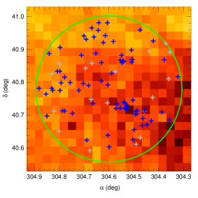
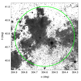
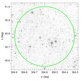
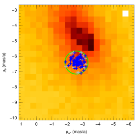
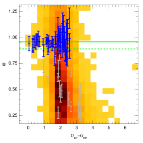
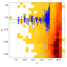
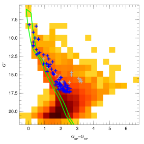
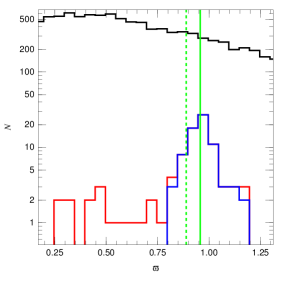
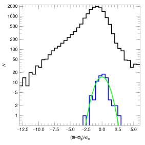
Figure 1: Collinder 419 Gaia DR2 distances and membership results. Top row (left to right): source density diagram, DSS2 Blue image, and 2MASS $J$ image. Middle row (left to right): proper motions, color-parallax, and magnitude-parallax diagrams. Bottom row (left to right): color-magnitude diagram, parallax histogram, and normalized-parallax histogram. In all diagrams a heat-type scale (increasing as white-yellow-orange-red-black) is used to indicate the total Gaia DR2 density in a linear scale (except in the CMD, where a log scale is used). In the first four panels the green circle indicates the coordinates/proper motions constraints. In the CMD the green lines show the reference extinguished isochrone (right) and the displaced one used as constraint (left), joined at the top by the extinction trajectory. In all diagrams blue symbols are used for the objects used in the final sample and gray ones for those rejected by the normalized parallax criterion. The plotted parallax uncertainties are the external ones. In the parallax histogram black is used for the total Gaia DR2 density, red for the sample prior to the application of the normalized parallax criterion, and blue for the final sample, while the two green vertical lines mark the weighted-mean parallax: dotted for $\varpi_{\rm g,0}$ and solid for $\varpi_{\rm g}$. Black and blue have the same meaning in the normalized parallax histogram, where the green line shows the expected normal distribution.

   

   

   

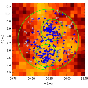
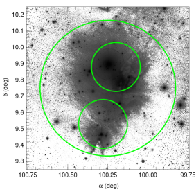
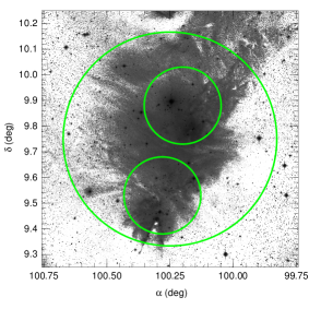
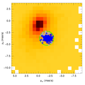
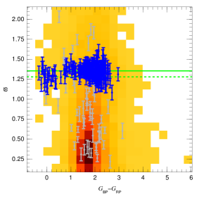
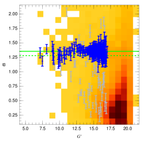
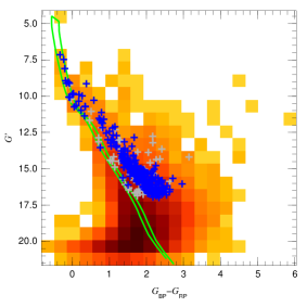
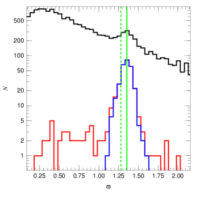
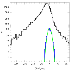
Figure 2: Same as Fig. 1 for NGC 2264 with two changes: the upper right panel shows a DSS2 Red image and two additional circles are used to mark the subgroups NGC 2264 N and NGC 2264 S in the top three panels.

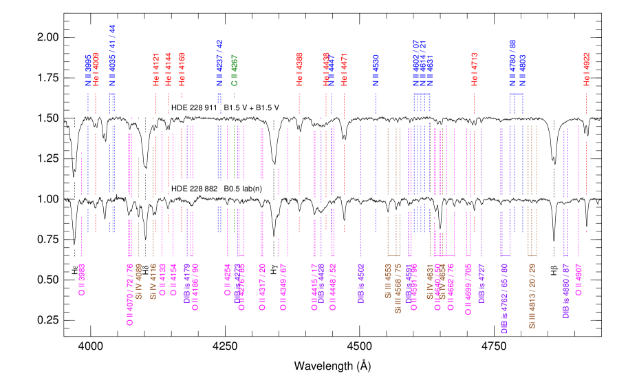
Figure 3: GOSSS spectrograms of HDE 228 911 and HDE 228 882.

 Collinder 419 appears in the top panels of Fig. 1 as a loosely defined cluster centered around HD 193 322, which is the brightest object on the field. The cluster core has a radius of $\sim$2′ but $r$ is significantly bigger, as the cluster has a larger halo that extends mostly towards the NE. With the possible exception of the immediate vicinity of HD 193 322, Collinder 419 does not show as an overdensity in the Gaia source density diagram. The vast majority of the sources belong to a Galactic background population at a distance of 2-5 kpc and they show a gradient increasing from NE to SW. That direction is nearly parallel to the Galactic plane, so the effect is likely caused by differential extinction beyond the distance of Collinder 419 and not by a real Galactic disk density gradient.

As Collinder 419 is not well defined by position in the sky, we must turn to the next panel in Fig. 1 to see its most defining characteristic, proper motion. The cluster is clearly separated from the field population by $\sim 2$ mas/a. The next three panels show how the cluster differs also in $G^{\prime}$ and $\mbox{$G_{\rm BP}$}-\mbox{$G_{\rm RP}$}$. The CMD indicates that Collinder 419 has a relatively low extinction: Maíz Apellániz & Barbá (2018) give $\mbox{$E(4405-5495)$}=0.381\pm 0.006$ and $\mbox{$R_{5495}$}=2.972\pm 0.079$ for HD 193 322 Aa,Ab, which translates into a $E(\mbox{$G_{\rm BP}$}-\mbox{$G_{\rm RP}$})\approx 0.65$. As I am selecting cluster objects with $\Delta(\mbox{$G_{\rm BP}$}-\mbox{$G_{\rm RP}$})>-0.30$, which corresponds to $E(\mbox{$G_{\rm BP}$}-\mbox{$G_{\rm RP}$})>0.35$, this means that there is just a small extinction restriction for a young cluster at the distance of HD 193 322 Aa,Ab. The location of some cluster members towards the left and right of the upper part of the reference extinguished isochrone indicates that there is a differential extinction effect of a few tens in $E(4405-5495)$ for the Collinder 419 cluster members. As one progresses down the CMD, the cluster members end up preferentially to the right of the reference extinguished isochrone, an indication that those lower-mass stars have not reached the main sequence yet.

Most of the field population is located at larger distances and consists of two subpopulations: the largest one is made out of faint stars in the lower left quadrant of the CMD that also form the two main density peaks in the color-parallax and magnitude-parallax diagrams. The second population are likely red giant stars that make up most of the stars to the right of the cluster sequence in the CMD. Such red giant stars are likely the main source for the 18 contaminants rejected by the normalized parallax criterion.

The distance I obtain for Collinder 419 is $1.006^{+0.037}_{-0.034}$ kpc, an uncertainty of 3-4%. Note that most of the uncertainty arises from the spatial covariance term: if it were not included $\sigma_{\varpi_{\rm g}}$ would be 6 $\mu$as instead of 34 $\mu$as (the spatial covariance is also the dominant source for the proper motion uncertainties). My value for $\varpi_{\rm g}$ is very similar to the one derived by Cantat-Gaudin et al. (2018) but the uncertainties are very different because of that. The two values for the distance are very similar, nonetheless (their mode is 1019.2 pc, within one sigma of the value here) but I find significantly more cluster members. With respect to the literature values, the Hipparcos distance for HD 193 322 Aa,Ab of Maíz Apellániz et al. (2008) is just over one sigma away (but with a large uncertainty) while the much lower distance of Roberts et al. (2010) derived from a pure CMD analysis is clearly incompatible with the Gaia parallaxes. Collinder 419 is not a rich cluster and, hence, is not able to make a dent in the total Gaia parallax histogram of Fig. 1. Indeed, only 0.4% of the Gaia stars in the field end up being selected by the algorithm. $t_{\varpi}$ is very close to one, indicating that the algorithm is identifying a group of stars with differences in distance much smaller than the individual parallax uncertainties. On the other hand, $t_{\mu_{\alpha*}}$ and $t_{\mu_{\delta}}$ are significantly larger than one, indicating that Gaia is sensitive to the internal cluster motions.

HD 193 322 Aa,Ab itself is not included in the final membership list as it was excluded due to its high RUWE, likely an effect of its multiplicity, which is unresolved by Gaia but should manifest in large astrometric residuals This should not worry us, as the method employed here emphasizes a low number of false positives at the price of increasing the number of false negatives. The second brightest (in $G^{\prime}$) object in the field, HD 193 159, is a foreground B star located at approximately one half the distance to Collinder 419 and with very little extinction. The third brightest object in the field is the first cluster member in the list: HD 193 322 B, the visual companion to HD 193 322 Aa,Ab. The next object in the membership list is HDE 228 911, a previously known spectroscopic binary. We obtained a GOSSS spectrum with the Albireo spectrograph at the Observatorio de Sierra Nevada (OSN) and caught the system in a SB2 state, allowing to determine it is made out of a couple of near identical B1.5 V stars (Fig. 3). The observation was obtained at HJD 2 455 850.283 and the velocity difference between the two components was 325$\pm$10 km/s. Another bright object in the field is HDE 228 882 but its Gaia DR2 parallax puts it beyond Collinder 419 and its $\mbox{$G_{\rm BP}$}-\mbox{$G_{\rm RP}$}$ color indicates it experiences a significantly larger extinction. We also obtained a GOSSS spectrum from OSN for HDE 228 882 and derived a spectral type of B0.5 Iab(n) (Fig. 3). Comparing the two spectra in that figure shows that the second one has stronger DIBs, as expected from the larger extinction. Roberts et al. (2010) suggested that 2MASS J20175763$+$4044373 (= IRAS 20161$+$4035) is also a cluster member and derived a spectral type of M3 III for that star, which appears in principle incompatible with the Collinder 419 isochrone. The Gaia DR2 data hold a surprise for the object: its individual parallax is consistent with being at the same distance as the cluster but its proper motion is highly discrepant with either Collinder 419 or the field population and instead suggests a relative velocity in the plane of the sky close to 50 km/s. This raises the possibility that 2MASS J20175763$+$4044373 is a recent runaway from Collinder 419. However, its motion does not trace back to HD 193 322 but to a region of high extinction towards the NE that appears to be associated to the WISE H ii region G078.378$+$02.785. Therefore, another possibility is that G078.378$+$02.785 is a younger star-forming region at the same distance (a second generation of stars likely triggered by Collinder 419) and that 2MASS J20175763$+$4044373 is a massive very young PMS object ejected from there $\sim 10^{5}$ a ago (as estimated from the flying time). The young age would be consistent with the strong Li i absorption in the spectrum of 2MASS J20175763$+$4044373 measured by Roberts et al. (2010).

3.2 NGC 2264

 The appearance of NGC 2264 in the top panels of Fig. 2 is different from that of Collinder 419 for four reasons: [1] there are significantly more cluster members, [2] NGC 2264 shows a clear double structure concentrated around two points, [3] the position of the cluster is well correlated with nebular emission, and [4] anti correlated with the overall source density. The last point seems counterintuitive but it can be explained in the context of the third one. Young clusters containing O stars still associated with their natal clouds ionize their surfaces creating H ii regions but take their time to devour their molecular clouds, generating different extinction-related effects and structures depending on the direction from where we observe them (Walborn et al., 2002; Maíz Apellániz et al., 2004, 2015; Maíz Apellániz & Barbá, 2018). The case of NGC 2264 is similar to that of the Orion Nebula: they are nearby, well resolved H ii regions where the main ionizing star (15 Mon for NGC 2264, $\theta^{1}$ Ori C for the Orion Nebula) is located on the near side of the natal cloud. Therefore, we see the H ii face on with the ionizing star(s) in the foreground. The H ii region has the overall shape of a concave hole in the molecular cloud, which results in a bright region surrounded by a dark one, with possible pillars created by photoevaporation at the edge. In the case of NGC 2264 the Cone Nebula (seen towards the bottom of the DSS2 images in Fig. 2) is the most prominent example. As the molecular cloud blocks most of the light behind the cluster, the field population (located mostly in the background at distances of 2-5 kpc) is much better seen at the right and left edges of the field shown in Fig. 2: hence, the anticorrelation between cluster members and overall source density.

As already mentioned, the double cluster structure of NGC 2264 in the optical was previously known, with two additional stellar concentrations visible in the NIR, indicating that there are additional hidden subclusters (Caballero & Dinis, 2008). In order to study the possible differences between the two subclusters (NGC 2264 N and NGC 2264 S), I have repeated the analysis of the whole region for the two subregions in Table 3 and plotted them in the upper panels of Fig. 2. NGC 2264 N is approximately centered on 15 Mon and NGC 2264 S is closer to the Cone Nebula.

As it happened with Collinder 419, NGC 2264 is best differentiated from the field population in the proper-motion diagram, with a separation of $\sim 3$ mas/a in Fig. 2. The CMD indicates that Collinder 419 has a very low extinction: Maíz Apellániz & Barbá (2018) give $\mbox{$E(4405-5495)$}=0.054\pm 0.006$ and $\mbox{$R_{5495}$}=4.431\pm 0.752$ for 15 Mon Aa,Ab,B, which translates into a $E(\mbox{$G_{\rm BP}$}-\mbox{$G_{\rm RP}$})\approx 0.11$. As I am selecting cluster objects with $\Delta(\mbox{$G_{\rm BP}$}-\mbox{$G_{\rm RP}$})>-0.20$, which corresponds to $E(\mbox{$G_{\rm BP}$}-\mbox{$G_{\rm RP}$})>-0.09$ (a negative value is used to include the effect of photometric uncertainties for objects with extinction close to zero), this means that there is no extinction restriction for a young cluster at the distance of 15 Mon Aa,Ab,B (but the isochrone filter is still useful to discard background objects). Going down the isochrone in the CMD we encounter first stars that have already reached the main sequence and then a pre-main sequence region that is richer and more separated from the isochrone than in the Collinder 419 case, indicating a younger age and likely a higher cluster mass. Note that the PMS seems to stop around $G^{\prime}$ = 18. This is likely an effect of the $d_{\rm CC}$ filter: dim stars immersed in nebulosity such as those in NGC 2264 have contaminated $G_{\rm BP}$ and $G_{\rm RP}$ photometry.

The field population is located mostly beyond NGC 2264. It is similar to that of Collinder 419 but with fewer stars at extreme red colors, an effect of the lower extinction in this direction of the Galaxy, much closer to the anticenter. Most of the 66 contaminants rejected by the normalized parallax criterion are farther than NGC 2264 but a minority (eight) are closer.

The distance we obtain for NGC 2264 is 719$\pm$16 pc (an uncertainty of just 2%). As with Collinder 419, most of the uncertainty arises from the spatial covariance term: if it were not included $\sigma_{\varpi_{\rm g}}$ would be 3 $\mu$as instead of 29 $\mu$as. Indeed, my value for $\varpi_{\rm g}$ is the same as the one derived by Cantat-Gaudin et al. (2018) but the uncertainties are very different because of that. I also find significantly more cluster members. With respect to the literature values, the maser distance of Kamezaki et al. (2014) is the one closer to the Gaia value, being less than one sigma away. NGC 2264 is a richer cluster and, hence, its presence is detected in the total Gaia parallax histogram of Fig. 2: 1.1% of the Gaia stars in the field end up being selected by the algorithm. Similarly to Collinder 419, $t_{\varpi}$ is close to one, but $t_{\mu_{\alpha*}}$ and $t_{\mu_{\delta}}$ are even larger, a sign that the internal motions are stronger in NGC 2264 (see below).

Comparing the two subclusters, their distances are very similar and from the Gaia DR2 point of view they could be at the same distance from the Sun. Note that their distance in the plane of the sky corresponds to 4.5 pc, which is much smaller than either of the individual distance uncertainties. There is a significant difference in the proper motions, with the two subclusters moving in a counterclockwise motion with respect to each other. This relative motion should in principle contribute to the increased values of $t_{\mu_{\alpha*}}$ and $t_{\mu_{\delta}}$ but it cannot be the main source, as both NGC 2264 N and NGC 2264 S (especially the latter) have high values of those quantities when analyzed separately. Therefore, one must conclude that the internal motions within each subcluster dominate the velocity dispersion.

Neither 15 Mon AaAb nor 15 Mon B are included in the final membership list due to their high RUWE but, as I already mentioned in the case of Collinder 419, that should not worry us. The second and third objects in the membership list (sorted by $G$) are HD 47 887 and HD 47 961, two B stars. Table 9 includes many more stars with spectral types than Table 8, a reflection of the different levels of richness and number of previous studies between the two clusters. Progressing down the list the spectral types progressively switch from B to A and then to later types, as expected. Nevertheless, it should be noted that one should not trust Simbad spectral types completely, given the number of errors it contains (see Maíz Apellániz et al. 2016 for some examples).

3.3 Testing the robustness of the distance determinations

 A critique to supervised methods is that the user may not select the appropriate parameters and bias the results. In order to check that the values for $\varpi_{\rm g}$ derived here are unbiased, I did Montecarlo simulations for the clusters in this paper varying the values of $\alpha$, $\delta$, $r$, $\mu_{\alpha*}$, $\mu_{\delta}$, $r_{\mu}$, and $\Delta(\mbox{$G_{\rm BP}$}-\mbox{$G_{\rm RP}$})$ within reasonable limits. For Collinder 419 the Montecarlo simulations yield $N_{*}=64\pm 16$ and $\mbox{$\varpi_{\rm g}$}=0.956\pm 0.004$ mas and for NGC 2264 they yield $N_{*}=253\pm 39$ and $\mbox{$\varpi_{\rm g}$}=1.354\pm 0.002$ mas. Those results lead to two conclusions. First, the number of Gaia-detected cluster members is within one sigma of our selected value but in both cases the average is on the low side. This makes sense because supervision is introduced, among other things, to maximize the number of bona fide members so removing the supervision decreases that number on average. Second, and most important, the group parallax is robust. The difference is 1 $\mu$as for Collinder 419 and even less than that for NGC 2264. Considering that the main source of error is due to the spatial covariance (more than one order of magnitude larger), I can conclude that supervision (if done properly) does not bias the derived group parallax.

4 The visual orbits of HD 193 322 Aa,Ab and 15 Mon Aa,Ab

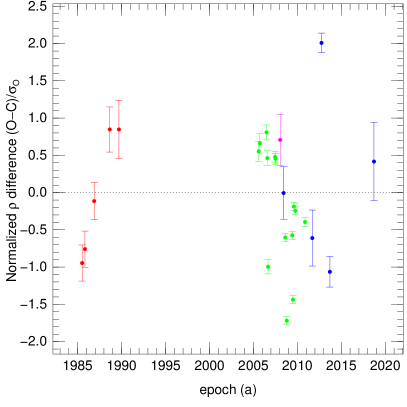
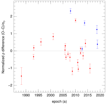
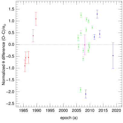
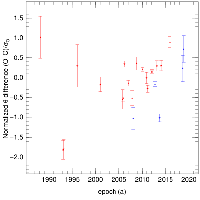
Figure 7: Normalized separation (top) and position angle (bottom) residue plots for HD 193 322 Aa,Ab (left) and 15 Mon Aa,Ab (right). The vertical position shows the residue position in the normalized O-C sense (data-fit divided by the individual observed uncertainties) and the vertical error bar shows the one-sigma range allowed by the fit. The color code is the same as in Fig. 4.

 In this section I present the results for the relative visual orbits for HD 193 322 Aa,Ab and 15 Mon Aa,Ab. The data used for the calculation of the orbits (including the uncertainties derived from the method itself) are given in Tables 4 and 5. I used the option of fitting $\varpi\equiv\omega+\Omega$ instead of $\omega$. The seven fitted parameters, $d$, $\omega$, and total masses $M_{\rm Aa,Ab}$ are given in Table 6. In each case a median and percentile-based uncertainties (derived from all calculated orbits) are first given, followed by the result for the mode orbit. For the masses I assume the distances to Collinder 419 and NGC 2264 derived in the previous section and do not include the uncertainties associated with distance. Figure 4 shows the fitted orbits, Figs. 5 and 6 the derived likelihood projected into the planes of each pair of fitted parameters, and Fig. 7 the normalized fitting residues. Table 7 gives the calculated ephemerides (and their uncertainties) for both systems in the period 1980-2030.

Table 4: Astrometry used for the calculation of the visual orbit of HD 193 322 Aa,Ab.

Epoch $\rho$ $\theta$ Reference (a) (mas) (deg) 1985.52 49.0$\pm$ 6.0 188.50$\pm$ 5.00 McAlister et al. (1987) 1985.84 49.0$\pm$ 6.0 192.60$\pm$ 5.00 McAlister et al. (1993) 1986.89 49.0$\pm$ 6.0 198.70$\pm$ 5.00 McAlister et al. (1989) 1988.66 48.0$\pm$ 6.0 216.70$\pm$ 5.00 McAlister et al. (1993) 1989.70 45.0$\pm$ 6.0 229.70$\pm$ 5.00 McAlister et al. (1993) 2005.60 63.8$\pm$ 6.0 109.10$\pm$ 5.00 ten Brummelaar et al. (2011) 2005.73 64.7$\pm$ 6.0 107.70$\pm$ 5.00 ten Brummelaar et al. (2011) 2006.49 67.0$\pm$ 6.0 101.50$\pm$ 5.00 ten Brummelaar et al. (2011) 2006.59 65.1$\pm$ 6.0 113.90$\pm$ 5.00 ten Brummelaar et al. (2011) 2006.67 56.5$\pm$ 6.0 118.00$\pm$ 5.00 ten Brummelaar et al. (2011) 2007.47 66.6$\pm$ 6.0 111.70$\pm$ 5.00 ten Brummelaar et al. (2011) 2007.51 66.5$\pm$ 6.0 113.60$\pm$ 5.00 ten Brummelaar et al. (2011) 2008.05 65.3$\pm$ 1.1 116.71$\pm$ 0.97 Aldoretta et al. (2015) 2008.44 65.0$\pm$ 1.0 113.45$\pm$ 2.21 Maíz Apellániz et al. (2019) 2008.62 61.6$\pm$ 6.0 121.80$\pm$ 5.00 ten Brummelaar et al. (2011) 2008.80 55.1$\pm$ 6.0 124.70$\pm$ 5.00 ten Brummelaar et al. (2011) 2009.42 62.6$\pm$ 6.0 120.10$\pm$ 5.00 ten Brummelaar et al. (2011) 2009.50 57.5$\pm$ 6.0 126.70$\pm$ 5.00 ten Brummelaar et al. (2011) 2009.61 65.1$\pm$ 6.0 122.00$\pm$ 5.00 ten Brummelaar et al. (2011) 2009.78 64.9$\pm$ 6.0 122.00$\pm$ 5.00 ten Brummelaar et al. (2011) 2010.87 64.8$\pm$ 6.0 129.80$\pm$ 5.00 ten Brummelaar et al. (2011) 2011.70 67.0$\pm$ 1.0 129.82$\pm$ 3.18 Maíz Apellániz et al. (2019) 2012.75 74.0$\pm$ 3.0 134.55$\pm$ 1.89 Maíz Apellániz et al. (2019) 2013.70 66.0$\pm$ 2.0 136.12$\pm$ 2.31 Maíz Apellániz et al. (2019) 2018.72 67.0$\pm$ 1.0 150.55$\pm$ 1.00 Maíz Apellániz et al. (2019)

Table 5: Astrometry used for the calculation of the visual orbit of 15 Mon Aa,Ab.

Epoch $\rho$ $\theta$ Reference (a) (mas) (deg) 1988.17 57.0$\pm$ 2.5 12.90$\pm$ 2.00 McAlister et al. (1993) 1993.09 39.0$\pm$ 5.0 35.40$\pm$ 6.00 McAlister et al. (1993) 1993.20 41.0$\pm$ 5.0 36.70$\pm$ 6.00 McAlister et al. (1993) 1996.07 22.3$\pm$ 5.0 115.90$\pm$ 6.00 Gies et al. (1997) 2001.02 61.0$\pm$ 5.0 231.10$\pm$ 6.00 Mason et al. (2009) 2005.82 89.0$\pm$ 2.5 247.90$\pm$ 2.00 Maíz Apellániz (2010) 2005.94 91.0$\pm$ 5.0 246.20$\pm$ 6.00 Horch et al. (2008) 2006.19 89.0$\pm$ 5.0 251.90$\pm$ 6.00 Mason et al. (2009) 2007.01 94.0$\pm$ 5.0 250.80$\pm$ 6.00 Horch et al. (2010) 2007.82 97.8$\pm$ 2.5 252.14$\pm$ 2.00 Aldoretta et al. (2015) 2008.04 109.0$\pm$ 4.0 252.26$\pm$ 1.29 Maíz Apellániz et al. (2019) 2008.78 100.0$\pm$ 2.5 255.63$\pm$ 2.00 Aldoretta et al. (2015) 2010.07 117.0$\pm$ 5.0 258.30$\pm$ 6.00 Mason et al. (2011) 2010.96 109.8$\pm$ 2.5 258.40$\pm$ 2.00 Hartkopf et al. (2012) 2011.18 108.5$\pm$ 3.5 257.92$\pm$ 2.89 Sana et al. (2014) 2012.10 116.1$\pm$ 5.0 261.00$\pm$ 6.00 Horch et al. (2017) 2012.10 114.8$\pm$ 5.0 260.90$\pm$ 6.00 Horch et al. (2017) 2012.75 118.0$\pm$ 4.0 260.30$\pm$ 3.80 Maíz Apellániz et al. (2019) 2013.13 118.0$\pm$ 2.5 262.00$\pm$ 2.00 Tokovinin et al. (2014) 2013.72 127.0$\pm$ 4.0 259.51$\pm$ 2.62 Maíz Apellániz et al. (2019) 2014.06 122.6$\pm$ 2.5 263.20$\pm$ 2.00 Tokovinin et al. (2015) 2015.91 124.0$\pm$ 2.5 266.60$\pm$ 2.00 Tokovinin et al. (2016) 2018.71 138.0$\pm$ 4.0 268.10$\pm$ 1.00 Maíz Apellániz et al. (2019) 2018.91 135.0$\pm$ 4.0 268.79$\pm$ 1.00 Maíz Apellániz et al. (2019)

Table 6: Fitted orbital parameters, $d$, $\omega$, and $M_{\rm Aa,Ab}$ for HD 193 322 Aa,Ab and 15 Mon Aa,Ab.

Par. Units HD 193 322 Aa,Ab 15 Mon Aa,Ab All Mode All Mode $P$ a 44${}^{+}_{-}$ ${}^{1}_{1}$ 44.1 108${}^{+}_{-}$ ${}^{12}_{12}$ 104.5 $T_{0}$ a 1995.2${}^{+}_{-}$ ${}^{1.2}_{0.8}$ 1995.3 1996.05${}^{+}_{-}$ ${}^{0.15}_{0.10}$ 1996.06 $e$ 0.58${}^{+}_{-}$ ${}^{0.03}_{0.04}$ 0.58 0.770${}^{+}_{-}$ ${}^{0.023}_{0.030}$ 0.764 $a$ mas 52.5${}^{+}_{-}$ ${}^{2.5}_{2.0}$ 52.4 112.5${}^{+}_{-}$ ${}^{6.0}_{6.0}$ 110.4 $i$ deg 37${}^{+}_{-}$ ${}^{6}_{4}$ 37.4 47${}^{+}_{-}$ ${}^{2}_{2}$ 47.3 $\Omega$ deg 77.6${}^{+}_{-}$ ${}^{12.0}_{14.4}$ 77.2 60${}^{+}_{-}$ ${}^{3}_{3}$ 60.2 $\varpi$ deg $-$30${}^{+}_{-}$ ${}^{6}_{6}$ $-$29.5 123${}^{+}_{-}$ ${}^{2}_{1}$ 123.2 $d$ mas 22.1${}^{+}_{-}$ ${}^{1.4}_{1.3}$ 22.1 26.0${}^{+}_{-}$ ${}^{1.3}_{1.5}$ 26.1 $\omega$ deg 253.6${}^{+}_{-}$ ${}^{9.2}_{9.2}$ 253.3 63${}^{+}_{-}$ ${}^{4}_{4}$ 62.9 $M_{\rm Aa,Ab}$ M_⊙ 76.1${}^{+}_{-}$ ${}^{9.9}_{7.4}$ 74.4 45.1${}^{+}_{-}$ ${}^{3.6}_{3.3}$ 45.9

 

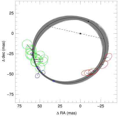
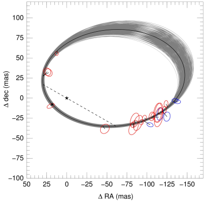
Figure 4: Plane-of-the-sky orbit plots for HD 193 322 Aa,Ab (left) and 15 Mon Aa,Ab (right). The mode (highest likelihood) orbit is shown as a thick black line, with a star marking the orbital center, a dashed line the line of nodes, and a cross the periastron. In both cases the motion is counterclockwise and less than a full revolution has been completed since the first data were obtained. In addition to the mode orbit, the top 1000 orbits by likelihood found by the algorithm are plotted using gray thin lines. Ellipses show the measured data points joined by short lines to the predicted position in the mode orbit. A color code is used to indicate the data source. For HD 193 322 Aa,Ab (Table 4), red is used for McAlister et al. (1989), green for ten Brummelaar et al. (2011), magenta for Aldoretta et al. (2015), and blue for Maíz Apellániz et al. (2019). For 15 Mon Aa,Ab (Table 5), blue is used for Maíz Apellániz et al. (2019) and red for the rest of the sources. North is up and East is left. Using the distances derived in this paper, the plotted regions are 126 AU $\times$ 126 AU for HD 193 322 Aa,Ab and 158 AU $\times$ 158 AU for 15 Mon Aa,Ab.

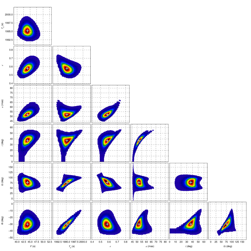
Figure 5: Likelihood plots of every parameter pair for the orbital fitting of HD 193 322 Aa,Ab. The levels plotted range between 0.1% and 100% of the maximum collapsed (from the other five parameters) likelihood in each case using a linear scale. The cross marks the projection of the seven-parameter mode into that plane (which does not necessary correspond to the maximum of the collapsed likelihood).

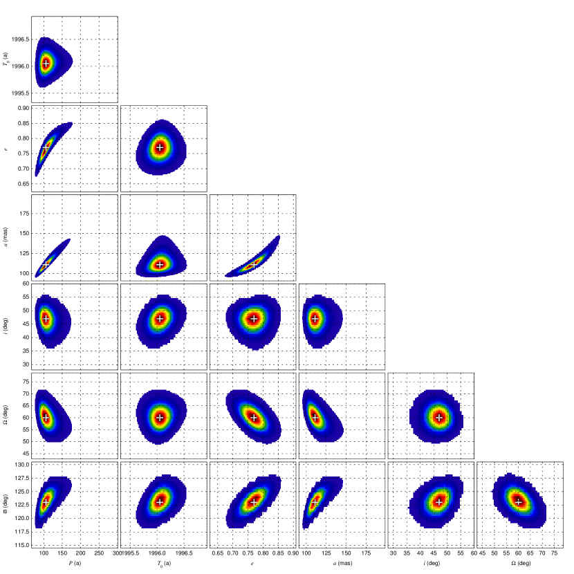
Figure 6: Same as Fig. 5 for 15 Mon Aa,Ab.

 

 

Table 7: Calculated ephemerides and their uncertainties for HD 193 322 Aa,Ab and 15 Mon Aa,Ab in the 1980-2030 period.

Epoch HD 193 322 Aa,Ab 15 Mon Aa,Ab $\rho$ $\theta$ $\rho$ $\theta$ (a) (mas) (deg) (mas) (deg) 1980.0 61.30$\pm$ 0.75 170.06$\pm$ 1.82 84.68$\pm$ 1.95 341.89$\pm$ 1.79 1981.0 59.95$\pm$ 0.79 174.01$\pm$ 1.81 81.96$\pm$ 1.89 344.55$\pm$ 1.70 1982.0 58.48$\pm$ 0.82 178.16$\pm$ 1.79 79.19$\pm$ 1.83 347.38$\pm$ 1.60 1983.0 56.89$\pm$ 0.84 182.52$\pm$ 1.78 76.37$\pm$ 1.76 350.43$\pm$ 1.51 1984.0 55.17$\pm$ 0.85 187.15$\pm$ 1.76 73.49$\pm$ 1.68 353.71$\pm$ 1.41 1985.0 53.32$\pm$ 0.85 192.09$\pm$ 1.75 70.54$\pm$ 1.59 357.26$\pm$ 1.31 1986.0 51.32$\pm$ 0.85 197.40$\pm$ 1.74 67.52$\pm$ 1.49 1.13$\pm$ 1.21 1987.0 49.14$\pm$ 0.87 203.16$\pm$ 1.74 64.42$\pm$ 1.38 5.36$\pm$ 1.13 1988.0 46.76$\pm$ 0.95 209.49$\pm$ 1.77 61.21$\pm$ 1.26 10.03$\pm$ 1.07 1989.0 44.10$\pm$ 1.14 216.54$\pm$ 1.83 57.85$\pm$ 1.13 15.22$\pm$ 1.05 1990.0 41.11$\pm$ 1.48 224.56$\pm$ 2.00 54.30$\pm$ 1.00 21.08$\pm$ 1.07 1991.0 37.66$\pm$ 2.01 233.98$\pm$ 2.45 50.45$\pm$ 0.87 27.79$\pm$ 1.14 1992.0 33.60$\pm$ 2.75 245.59$\pm$ 3.62 46.17$\pm$ 0.76 35.68$\pm$ 1.26 1993.0 28.80$\pm$ 3.62 261.06$\pm$ 6.61 41.19$\pm$ 0.71 45.32$\pm$ 1.43 1994.0 23.59$\pm$ 4.00 284.09$\pm$ 13.72 35.12$\pm$ 0.74 57.97$\pm$ 1.67 1995.0 19.82$\pm$ 2.71 318.29$\pm$ 22.99 27.61$\pm$ 0.87 76.82$\pm$ 2.06 1996.0 19.95$\pm$ 2.26 357.70$\pm$ 24.42 20.07$\pm$ 0.99 110.70$\pm$ 3.09 1997.0 24.06$\pm$ 4.12 30.59$\pm$ 17.30 19.57$\pm$ 0.73 162.50$\pm$ 4.30 1998.0 30.07$\pm$ 4.65 52.62$\pm$ 9.68 27.78$\pm$ 0.85 197.66$\pm$ 3.02 1999.0 36.15$\pm$ 4.23 66.82$\pm$ 5.39 38.06$\pm$ 0.96 215.11$\pm$ 2.01 2000.0 41.59$\pm$ 3.54 76.78$\pm$ 3.25 47.83$\pm$ 0.97 225.20$\pm$ 1.46 2001.0 46.30$\pm$ 2.86 84.44$\pm$ 2.11 56.68$\pm$ 0.94 231.97$\pm$ 1.13 2002.0 50.32$\pm$ 2.27 90.72$\pm$ 1.45 64.65$\pm$ 0.89 236.98$\pm$ 0.91 2003.0 53.76$\pm$ 1.76 96.10$\pm$ 1.06 71.85$\pm$ 0.83 240.94$\pm$ 0.75 2004.0 56.68$\pm$ 1.33 100.88$\pm$ 0.81 78.38$\pm$ 0.77 244.20$\pm$ 0.64 2005.0 59.17$\pm$ 0.99 105.21$\pm$ 0.65 84.36$\pm$ 0.72 246.98$\pm$ 0.54 2006.0 61.26$\pm$ 0.72 109.22$\pm$ 0.54 89.83$\pm$ 0.66 249.41$\pm$ 0.47 2007.0 63.01$\pm$ 0.51 112.98$\pm$ 0.47 94.88$\pm$ 0.60 251.57$\pm$ 0.41 2008.0 64.46$\pm$ 0.38 116.55$\pm$ 0.41 99.54$\pm$ 0.55 253.51$\pm$ 0.36 2009.0 65.63$\pm$ 0.33 119.98$\pm$ 0.37 103.86$\pm$ 0.50 255.29$\pm$ 0.33 2010.0 66.55$\pm$ 0.33 123.31$\pm$ 0.34 107.87$\pm$ 0.47 256.93$\pm$ 0.30 2011.0 67.25$\pm$ 0.36 126.55$\pm$ 0.33 111.61$\pm$ 0.44 258.46$\pm$ 0.27 2012.0 67.74$\pm$ 0.38 129.74$\pm$ 0.32 115.08$\pm$ 0.44 259.89$\pm$ 0.26 2013.0 68.03$\pm$ 0.40 132.89$\pm$ 0.33 118.32$\pm$ 0.46 261.24$\pm$ 0.25 2014.0 68.14$\pm$ 0.41 136.02$\pm$ 0.35 121.34$\pm$ 0.51 262.52$\pm$ 0.26 2015.0 68.09$\pm$ 0.42 139.15$\pm$ 0.38 124.15$\pm$ 0.58 263.74$\pm$ 0.26 2016.0 67.88$\pm$ 0.43 142.30$\pm$ 0.41 126.78$\pm$ 0.66 264.91$\pm$ 0.28 2017.0 67.52$\pm$ 0.45 145.46$\pm$ 0.46 129.23$\pm$ 0.76 266.03$\pm$ 0.29 2018.0 67.03$\pm$ 0.49 148.67$\pm$ 0.51 131.51$\pm$ 0.87 267.12$\pm$ 0.31 2019.0 66.39$\pm$ 0.54 151.94$\pm$ 0.56 133.63$\pm$ 0.99 268.16$\pm$ 0.34 2020.0 65.63$\pm$ 0.62 155.27$\pm$ 0.63 135.60$\pm$ 1.12 269.18$\pm$ 0.36 2021.0 64.75$\pm$ 0.71 158.69$\pm$ 0.71 137.43$\pm$ 1.26 270.16$\pm$ 0.39 2022.0 63.75$\pm$ 0.81 162.21$\pm$ 0.80 139.13$\pm$ 1.40 271.13$\pm$ 0.42 2023.0 62.64$\pm$ 0.92 165.85$\pm$ 0.91 140.69$\pm$ 1.55 272.07$\pm$ 0.45 2024.0 61.41$\pm$ 1.04 169.63$\pm$ 1.04 142.14$\pm$ 1.71 272.99$\pm$ 0.49 2025.0 60.06$\pm$ 1.16 173.57$\pm$ 1.19 143.46$\pm$ 1.87 273.89$\pm$ 0.52 2026.0 58.60$\pm$ 1.28 177.70$\pm$ 1.38 144.67$\pm$ 2.03 274.78$\pm$ 0.56 2027.0 57.03$\pm$ 1.41 182.06$\pm$ 1.60 145.77$\pm$ 2.20 275.65$\pm$ 0.60 2028.0 55.33$\pm$ 1.52 186.67$\pm$ 1.87 146.76$\pm$ 2.38 276.51$\pm$ 0.64 2029.0 53.50$\pm$ 1.64 191.59$\pm$ 2.18 147.65$\pm$ 2.56 277.36$\pm$ 0.68 2030.0 51.52$\pm$ 1.77 196.88$\pm$ 2.56 148.45$\pm$ 2.75 278.20$\pm$ 0.72

4.1 HD 193 322 Aa,Ab

 The orbital solution I obtain for HD 193 322 Aa,Ab is relatively similar to the one derived by ten Brummelaar et al. (2011) but with some significant differences. On the one hand, the values of $T_{0}$ and $a$ are within one sigma of each other, with improved uncertainties in the new solution. On the other hand, the period is now longer and the orbit is more eccentric, a consequence of the better position angle coverage available now. Another significant difference is that I find a larger uncertainty for the inclination. An explanation to that is found in Fig. 5: most plots are relatively well approximated by ellipsoids but those involving $i$ have more complex shapes, including a low-probability tail that extends to low values. Such shapes cannot be described just by the derivatives at the location of the mode and correctly characterizing them requires a method that searches the seven-parameter space such as the one used here. Most parameters have low correlation coefficients but there are some exceptions, most notably $a$ and $i$, which are positively correlated. There is clearly room for improvement in the orbit, especially as one revolution has not been completed since the first observations (that event would take place by the end of the decade of the 2020s, Table 7) and since there were no observations in the 1990s, when the periastron took place. The next periastron will take place in about twenty years from now.

Applying a distance of 1006 pc to the ten Brummelaar et al. (2011) results, one obtains a total mass of $133\pm 29$ M_⊙, which is almost twice of what I obtain here. The new value is more realistic, as it requires dividing 76.1 M_⊙ among three non-supergiant late-O/early-B stars. The total mass was not such a big problem for ten Brummelaar et al. (2011) because they estimated Collinder 419 to be closer to us and that reduces $M_{\rm Aa,Ab}$, which is proportional to the distance cubed. Indeed, they were aware of this possibility as they mentioned the need for further epochs to resolve the “lingering problems” they had encountered with their mass calculations. Note that since our value for the distance to Collinder 419 has an uncertainty of 3-4%, the uncertainty for $M_{\rm Aa,Ab}$ has an additional (systematic) uncertainty of $\sim$10% i.e. comparable to the random uncertainty. Once Gaia DR3 becomes available, it is likely that systematic uncertainty will be reduced.

The ephemerides in Table 7 were calculated using the 1000 most likely orbits plotted in Fig. 4. The uncertainties in $\rho$ and $\theta$ show two minima, one in the second half of the 1980s and another one around 2010. Those are the two times where observations were obtained. In between, there is a large increase in uncertainties around the time of the periastron, as the system was moving at maximum speed at the time and no observations are available. Hence, there is a large uncertainty as to where the system was at a particular time even if the periastron is well constrained within $\sim$1 year. As we go into the future, uncertainties start growing again as the trajectory is an extrapolation from the latest data. Even though it is not shown, uncertainties continue growing until the next periastron passage around 2040 for the same reasons stated for the previous one.

Finally, I considered the possibility that the observations taken in the 1980s suffered from the 180° phase error in position angle that sometimes affects speckle interferometry. I was able to calculate a reasonable orbit combining those modified data with the ones from 2005 onwards but the resulting $M_{\rm Aa,Ab}$ was almost one third lower than the value in Table 6. That is an unphysical result, as it is inconsistent with the existence of three massive stars that include at least two O stars. Therefore, I conclude that the 1980s observations have no phase error.

4.2 15 Mon Aa,Ab

 As I mentioned in the introduction, for 15 Mon Aa,Ab there are five published orbital solutions instead of just one. Looking at them, there is a clear trend of increasing periods from those published in the 1990s to the most recent one of Tokovinin (2018) by more than a factor of five between the extremes. That effect is a cautionary tale on the dangers of calculating visual orbits from very incomplete arcs, especially if a thorough search of the parameter space is not performed and/or bad data points are not eliminated or at least down weighted. The orbital period I find here follows the trend of increasing periods of Gies et al. (1993, 1997) and Cvetković et al. (2009, 2010) but stops at a value that is just over one half of the Tokovinin (2018) value (which is published without uncertainties). The uncertainty in the period is relatively large ($\sim$10%) and there is indeed a tail that extends to higher values but the likelihood around 190 a is very low (Fig. 6). The new periastron epoch and eccentricity are similar to those of the previous three orbits but with reduced uncertainties. The values for $a$ and $i$ follow the same pattern as the period, with values intermediate between those of Cvetković et al. (2009, 2010) and Tokovinin (2018).

The mass derived for 15 Mon Aa,Ab has a relative uncertainty of less than 10%, which looks surprising given the uncertainties for $P$ and $a$, the two quantities used to derive it. The explanation is that $P$ and $a$ have a strong positive correlation, as seen in Fig.  6. The uncertainty on the distance to NGC 2264 is lower than for Collinder 419, leading to an additional systematic uncertainty of $\sim$7%. Nevertheless, the uncertainty for $M_{\rm Aa,Ab}$ is one of the lowest known for an O-type binary, especially considering that most measured systems to date are spectroscopic binaries with poorly constrained inclinations. The total mass we obtain (at a distance of 719 pc) is higher than the one derived by Gies et al. (1997) and lower than the one derived by Cvetković et al. (2010). It is relatively similar to the value derived from the Tokovinin (2018) orbit but that author does not calculate it explicitly.

The uncertainties for the 15 Mon Aa,Ab ephemerides in Table 7 follow a pattern similar to the HD 193 322 Aa,Ab, with two minima around 1990 and 2012. The maximum in between is not as prominent, though, as in this case the system was observed near periastron. As deduced from Fig. 4, the uncertainties are expected to grow significantly after 2040, as that part of the orbit near apastron has never been observed. On the other hand, observations in the next decade should constrain the orbital parameters significantly, even though the system will not return to its first observed epoch until around the turn of the century.

5 Future work

 My short-term goal is to apply the supervised Gaia method to a number of young clusters containing O stars in order to derive reliable Gaia DR2 distances. The clusters will be selected using GOSSS data and Maíz Apellániz & Barbá (2018) will be used for the extinction parameters. In the medium term, Gaia DR3 is expected to reduce the systematic effects in the parallaxes and proper motions, especially the zero point offset and the spatial covariance effects. Those reductions should lead to significantly better distances to stellar clusters. In the long term, the final Gaia data release may yield parallaxes good enough to measure distance differences within associations or cluster halos at $\sim$1 kpc.

Regarding astrometric orbits, I plan to use the existing data to analyze several more systems. I will also continue obtaining new AstraLux epochs to further constrain the HD 193 322 Aa,Ab and 15 Mon Aa,Ab orbits.

There is also room for improvement in our knowledge of HD 193 322 Aa,Ab and 15 Mon Aa,Ab elsewhere. We are monitoring both systems using high-resolution spectroscopy to improve their spectroscopic orbits as part of MONOS (Maíz Apellániz et al., 2019). However, there is a limit to what we can do with spatially unresolved spectroscopy, especially when one of the systems is a fast rotator or the $\Delta m$ between components is large. One solution would be lucky spectroscopy (Maíz Apellániz et al., 2018) but, unfortunately, the separation is too small. We recently attempted resolving 15 Mon Aa,Ab using that technique but we were only partially successful. It was possible to separate Ab from Aa but the resulting spectrum is too noisy and one can only say that it is consistent with being a late-O/early-B star. An alternative would be using STIS@HST, a technique we successfully used to separate HD 93 129 Aa,Ab at a point where the separation was even smaller than for the two systems in this paper (Maíz Apellániz et al., 2017). In that way, it would be possible to obtain individual spectra for HD 193 322 Aa, 15 Mon Aa, and 15 Mon Ab, and a combined spectrum for HD 193 322 Ab1,Ab2 that could be separated in velocity. In combination with the results in this paper, reliable spectral types and masses could be derived for all components. As this paper was being refereed we received notice that the HST program we had submitted to do precisely that had been accepted so, barring unexpected events, the reader should expect new results on these two systems soon.

Table 8: Collinder 419 Gaia DR2 selected sample sorted by $G$. S/G indicates the origin of the spectral type: (S)imbad or (G)OSSS. Quoted uncertainties are internal ones and $G$ is uncorrected. This is a short version of the full table with only the stars with spectral types. The full table is available in electronic form at the CDS via anonymous ftp to cdsarc.u-strasbg.fr (130.79.128.5) or via http://cdsweb.u-strasbg.fr/cgi-bin/qcat?J/A+A/.

Star	Gaia DR2 ID	2MASS ID	$\varpi$		$\mu_{\alpha*}$		$\mu_{\delta}$		$G$		$G_{\rm BP}$$-$$G_{\rm RP}$		Spectral	S/G
			(mas)		(mas/a)		(mas/a)						type
HD 193 322 B	2062360626009209856	-	0.9406$\pm$	0.0503	$-$2.851$\pm$	0.072	$-$6.345$\pm$	0.085	8.1681$\pm$	0.0011	0.0503$\pm$	0.0690	B1.5 V(n)p	G
HDE 228 911	2068355713159146112	J20192172$+$4053164	0.9440$\pm$	0.0354	$-$2.394$\pm$	0.056	$-$5.980$\pm$	0.065	8.3776$\pm$	0.0007	0.4752$\pm$	0.0024	B1.5 V + B1.5 V	G
HDE 228 845	2068367812086551936	J20182744$+$4056329	0.9570$\pm$	0.0328	$-$2.929$\pm$	0.047	$-$6.056$\pm$	0.048	9.1975$\pm$	0.0003	0.2993$\pm$	0.0019	B5	S
HDE 228 810	2062359015408118528	J20175865$+$4042097	0.9562$\pm$	0.0349	$-$2.675$\pm$	0.051	$-$6.377$\pm$	0.057	9.9835$\pm$	0.0003	0.4010$\pm$	0.0012	A2	S
HDE 228 903	2068355163403333504	J20191127$+$4050028	1.0069$\pm$	0.0280	$-$2.640$\pm$	0.049	$-$6.384$\pm$	0.049	10.1960$\pm$	0.0027	0.6229$\pm$	0.0116	B5	S
UCAC2 46029301	2062359152847218432	J20180562$+$4043248	0.9162$\pm$	0.0409	$-$2.727$\pm$	0.057	$-$6.458$\pm$	0.056	11.0201$\pm$	0.0014	0.2930$\pm$	0.0067	B8 V	S

Table 9: NGC 2264 Gaia DR2 selected sample sorted by $G$. S/G indicates the origin of the spectral type: (S)imbad or (G)OSSS. Quoted uncertainties are internal ones and $G$ is uncorrected. N/S indicates whether the star is in the northern/southern subclusters. This is a short version of the full table with only the brightest stars with spectral types. The full table is available in electronic form at the CDS via anonymous ftp to cdsarc.u-strasbg.fr (130.79.128.5) or via http://cdsweb.u-strasbg.fr/cgi-bin/qcat?J/A+A/.

Star	Gaia DR2 ID	2MASS ID	$\varpi$		$\mu_{\alpha*}$		$\mu_{\delta}$		$G$		$G_{\rm BP}$$-$$G_{\rm RP}$		Spectral	S/G	N/S
			(mas)		(mas/a)		(mas/a)						type
HD 47 887	3326686263650895360	J06410959$+$0927574	1.3272$\pm$	0.0705	$-$2.814$\pm$	0.126	$-$4.055$\pm$	0.106	7.1547$\pm$	0.0010	$-$0.3269$\pm$	0.0053	B2 III:	S	S
HD 47 961	3326737120359493504	J06412730$+$0951145	1.1831$\pm$	0.0691	$-$1.928$\pm$	0.119	$-$4.368$\pm$	0.109	7.4799$\pm$	0.0006	$-$0.2312$\pm$	0.0023	B2.5 V	S	-
V641 Mon	3326716813754146176	J06402858$+$0949042	1.3910$\pm$	0.0635	$-$2.061$\pm$	0.110	$-$3.937$\pm$	0.092	8.1115$\pm$	0.0010	$-$0.1989$\pm$	0.0036	B1.5 IV + B2 V:	S	N
HD 48 055	3326644967541579776	J06414970$+$0930293	1.4362$\pm$	0.0734	$-$2.426$\pm$	0.119	$-$4.114$\pm$	0.099	8.9462$\pm$	0.0009	$-$0.1804$\pm$	0.0030	B3 V	S	-
HDE 261 810	3326715439364610816	J06404322$+$0946017	1.2843$\pm$	0.0706	$-$2.297$\pm$	0.121	$-$3.880$\pm$	0.107	9.0346$\pm$	0.0005	$-$0.1044$\pm$	0.0028	B1	S	N
HDE 261 878	3326717260430731648	J06405155$+$0951494	1.3997$\pm$	0.0579	$-$1.512$\pm$	0.097	$-$4.083$\pm$	0.083	9.1140$\pm$	0.0006	$-$0.1567$\pm$	0.0022	B6 V	S	N
HDE 261 903	3326685924349755520	J06410288$+$0927234	1.2358$\pm$	0.0677	$-$1.714$\pm$	0.123	$-$3.603$\pm$	0.105	9.1224$\pm$	0.0008	$-$0.0752$\pm$	0.0026	B8 Vn	S	S
HDE 261 736	3326714919673593856	J06402475$+$0946082	1.1917$\pm$	0.0471	$-$1.703$\pm$	0.080	$-$3.949$\pm$	0.069	9.1537$\pm$	0.0006	0.3803$\pm$	0.0026	A5/7	S	N
HDE 262 066	3326736811121849216	J06413009$+$0949471	1.3020$\pm$	0.0733	$-$1.315$\pm$	0.108	$-$3.814$\pm$	0.093	9.8227$\pm$	0.0005	0.0276$\pm$	0.0028	A2	S	-
HDE 262 177	3326748802670510336	J06415108$+$1001448	1.1376$\pm$	0.0609	$-$1.397$\pm$	0.095	$-$3.902$\pm$	0.088	9.8571$\pm$	0.0007	0.0304$\pm$	0.0024	A0/1	S	-
HDE 262 108	3326737051640013952	J06413461$+$0951378	1.2346$\pm$	0.0437	$-$1.174$\pm$	0.075	$-$4.001$\pm$	0.064	9.8975$\pm$	0.0006	0.1846$\pm$	0.0037	A2/3	S	-
HDE 261 969	3326740006577519360	J06411038$+$0953018	1.1663$\pm$	0.0611	$-$1.773$\pm$	0.100	$-$4.213$\pm$	0.093	9.9047$\pm$	0.0006	$-$0.0007$\pm$	0.0016	B9 IV	S	N
HDE 261 841	3326717226070995328	J06404888$+$0951444	1.2982$\pm$	0.0481	$-$1.662$\pm$	0.084	$-$3.674$\pm$	0.073	9.9935$\pm$	0.0011	0.2683$\pm$	0.0048	B8 IV-Ve	S	N
HDE 261 940	3326695854314127616	J06410411$+$0933018	1.2855$\pm$	0.0721	$-$1.857$\pm$	0.137	$-$4.236$\pm$	0.111	10.0653$\pm$	0.0008	$-$0.0666$\pm$	0.0024	B6/9	S	S
HDE 261 936	3326941865743978880	J06410863$+$1008253	1.2022$\pm$	0.0826	$-$1.742$\pm$	0.135	$-$3.289$\pm$	0.112	10.0809$\pm$	0.0010	$-$0.0926$\pm$	0.0038	B6/9	S	-
NGC 2264 181	3326740002281694592	J06411123$+$0952556	1.3478$\pm$	0.0561	$-$1.478$\pm$	0.096	$-$3.856$\pm$	0.091	10.0922$\pm$	0.0005	$-$0.0610$\pm$	0.0023	B9 Vn	S	N
HDE 261 902	3326695923033606912	J06405851$+$0933317	1.0156$\pm$	0.0561	$-$1.381$\pm$	0.103	$-$4.026$\pm$	0.087	10.2098$\pm$	0.0005	$-$0.0324$\pm$	0.0019	B8	S	S
HDE 261 937	3326741277887838080	J06410456$+$0954438	1.2742$\pm$	0.0605	$-$1.210$\pm$	0.110	$-$3.968$\pm$	0.103	10.2985$\pm$	0.0010	0.5837$\pm$	0.0028	kA2hA2mA5 V	S	N
BD $+$09 1340	3326686508465460736	J06410155$+$0928130	1.3240$\pm$	0.0595	$-$1.334$\pm$	0.120	$-$3.932$\pm$	0.105	10.6613$\pm$	0.0004	0.1047$\pm$	0.0014	A0	S	S
NGC 2264 VAS 90	3326740865570981632	J06405893$+$0954008	1.3627$\pm$	0.0459	$-$1.137$\pm$	0.080	$-$3.589$\pm$	0.074	10.7189$\pm$	0.0006	0.3436$\pm$	0.0022	A3 V	S	N
HDE 261 809	3326936990957883008	J06404329$+$1008305	1.2094$\pm$	0.0558	$-$0.814$\pm$	0.088	$-$3.159$\pm$	0.072	10.7413$\pm$	0.0004	0.3519$\pm$	0.0016	A0/1	S	-
HDE 261 941	3326684653039444480	J06410587$+$0922556	1.2997$\pm$	0.0642	$-$1.709$\pm$	0.119	$-$3.742$\pm$	0.092	10.9899$\pm$	0.0012	0.2371$\pm$	0.0043	A2/3	S	S
NGC 2264 VAS 196	3326723101586583168	J06414302$+$0943324	2.0320$\pm$	0.0533	$-$2.707$\pm$	0.092	$-$4.503$\pm$	0.078	11.0624$\pm$	0.0005	0.5110$\pm$	0.0011	F0/2	S	-
NGC 2264 LBM 1668	3326703619614642560	J06400565$+$0935492	1.3520$\pm$	0.0336	$-$1.602$\pm$	0.062	$-$3.513$\pm$	0.057	11.1388$\pm$	0.0005	0.7876$\pm$	0.0019	F5 V	S	-
NGC 2264 104	3326740998714107008	J06404953$+$0953230	1.3462$\pm$	0.0413	$-$1.464$\pm$	0.074	$-$3.581$\pm$	0.064	11.3790$\pm$	0.0005	0.3291$\pm$	0.0023	A5 IV	S	N
NGC 2264 116	3326689807000188032	J06405377$+$0930389	1.3673$\pm$	0.0421	$-$2.161$\pm$	0.077	$-$3.796$\pm$	0.065	11.5432$\pm$	0.0003	0.7210$\pm$	0.0017	F7 V	S	S
NGC 2264 68	3326905478782410368	J06403749$+$0954578	1.3465$\pm$	0.0436	$-$1.556$\pm$	0.076	$-$3.500$\pm$	0.064	11.6125$\pm$	0.0008	0.8503$\pm$	0.0034	G0	S	N
NGC 2264 118	3326682552799138176	J06405435$+$0920045	1.2629$\pm$	0.0512	$-$2.127$\pm$	0.085	$-$3.564$\pm$	0.072	11.6650$\pm$	0.0004	0.7554$\pm$	0.0033	F8 V	S	-
GSC 00750-01657	3326731996461275904	J06422750$+$0952549	0.9174$\pm$	0.0728	$-$3.046$\pm$	0.092	$-$3.512$\pm$	0.079	11.6842$\pm$	0.0004	0.4709$\pm$	0.0026	A2/3	S	-
NGC 2264 84	3326691009590655616	J06404218$+$0933374	1.4321$\pm$	0.0404	$-$1.575$\pm$	0.074	$-$3.675$\pm$	0.062	11.8486$\pm$	0.0015	0.7920$\pm$	0.0077	G0	S	S