Assessment and optimization of the fast inertial relaxation engine (fire) for energy minimization in atomistic simulations and its implementation in lammps

Abstract

In atomistic simulations, pseudo-dynamics relaxation schemes often exhibit better performance and accuracy in finding local minima than line-search-based descent algorithms like steepest descent or conjugate gradient. Here, an improved version of the fast inertial relaxation engine (fire) and its implementation within the open-source atomistic simulation code lammps is presented. It is shown that the correct choice of time integration scheme and minimization parameters is crucial for the performance of fire.

1 Introduction

Numerical optimization [1, 2] is of utmost importance in almost every field of science and engineering. It is routinely used in atomistic simulations in condensed matter physics, physical chemistry, biochemistry, and materials science. There, the optimized quantity is usually the potential energy $E(\mathbf{x})$, for a given interatomic interaction model [3]. Minimizing $E(\mathbf{x})$ with respect to the atomic coordinates $\mathbf{x}$ yields 0 K equilibrium structures and energies, e.g., of defects. Minimum energy configurations can, furthermore, be used as initial states for subsequent molecular dynamics (md) simulations or normal-mode analyses [4]. Energy minimization is also used to determine the stability of structures under load. Two typical examples are the computation of the Peierls stress required for dislocation glide [5], and the determination of the critical stress intensity factor required for crack propagation [6]. Other uses of energy minimization methods in atomistic simulations include the search for transition states, e.g. by the nudged-elastic-band (neb) method [7], or the detection of transitions in accelerated md methods like parallel-replica dynamics or hyperdynamics [8].

Most atomistic simulation packages like lammps [9], gromacs [10], imd [11], dl_poly [12], eon [13] or ase [14] implement line-search-based descent algorithms like Steepest Descent (sd) or Conjugated Gradient (cg), as well as damped-dynamics methods like Microconvergence [15], Quickmin [16] and the Fast Inertial Relaxation Engine (fire) [17]. More complex algorithms including Quasi-Newton methods like the highly-efficient Limited-memory Broyden-Fletcher-Goldfarb-Shanno (l-bfgs) approach that involve the computation of the Hessian [2] are mostly used in ab-initio simulations and are not as widely implemented in atomistic simulations packages as the aforementioned Hessian-free algorithms.

fire is often used in atomistic simulations of mechanical properties of metals and alloys [6, 18], ceramics [19], polymers [20], carbon allotropes [21], amorphous materials [22] and granular media [23], as well as in simulations related to catalysis [24] or docking [25]. The strict adherence to force minimization in fire makes it ideally suitable for critical point analysis in translational invariant systems like for the determination of the Peierls stress of a dislocation [5, 17], where line-search-based descent algorithms often fail. Furthermore, fire has been shown to be a convenient algorithm for mapping basins of attraction, as it avoids unusual pathologies like disconnected basins of attraction that can appear, e.g., using the l-bfgs method [26]. fire was also shown to be a fast and computationally efficient minimizer for neb [7], as well as for the activation-relaxation technique (art) [27].

Here, we study the influence of the numerical integration scheme and the choice of parameters set (mixing coefficient, initial timestep, maximum timestep, etc.) on the efficiency of fire for different scenarios. We furthermore suggest a modification of the fire algorithm to improve its efficiency and describe our implementation of this modified version fire 2.0 in the atomistic simulation code lammps [9].

2 The algorithms

2.1 fire

Consider a system of $N$ particles with coordinates $\mathbf{x}\equiv(x_{1},x_{2},\dots,x_{3N})$ and mass $m$. The potential energy $E(\mathbf{x})$ depends only on the relative positions of the particles and can thus be envisioned as a $(3N-6)$-dimensional surface or “landscape”. The principle of fire is to perform dynamics which allow only for downhill motion on this landscape, with the acceleration

$$\mathbf{\dot{v}}(t)=\frac{\mathbf{F}(\mathbf{x}(t))}{m}-\gamma(t)|\mathbf{v}(t)|\left(\mathbf{\hat{v}}(t)-\mathbf{\hat{F}}(\mathbf{x}(t))\right).$$ (1)

Here, $t$ denotes time, $\mathbf{v}(t)$ the velocity of the particles ($\mathbf{v}(t)\equiv\mathbf{\dot{x}}(t)$), $\mathbf{F}(\mathbf{x}(t))$ the force acting on them, i.e., the gradient of the potential energy ($\mathbf{F}(\mathbf{x}(t))=-\nabla E(\mathbf{x}(t))$), and $\gamma(t)$ a scalar function of time. Boldface quantities denote vectors, hats indicate unit vectors, and $|\dots|$ is the Euclidean norm of the enclosed vector. The first term on the right hand side in equation 1 represents regular Newtonian dynamics. The effect of the second term is to reduce the angle between $\mathbf{v}(t)$ and $\mathbf{F}(\mathbf{x}(t))$, which is the direction of steepest descent at $\mathbf{x}(t)$. Uphill motion is avoided by computing the power $P(t)=\mathbf{F}(\mathbf{x}(t))\cdot\mathbf{v}(t)$ and setting the velocity to zero whenever $P(t)\leq 0$. It was shown that combining equation 1 with an adaptive time stepping scheme yields a simple and competitive optimization algorithm [17]. In practice, equation 1 is implemented by “mixing” $\mathbf{v}(t)$ and $\mathbf{F}(\mathbf{x}(t))$, using an adaptive mixing factor $\alpha(t)\in[0,1]$. The algorithm can then be written as proposed in Algorithm 1.

Algorithm 1 fire

1:Initialize $\mathbf{x}(t)$ and $\mathbf{F}(\mathbf{x}(t))$

2:$\mathbf{v}(t)\leftarrow 0$

3:$\alpha\leftarrow\alpha_{\mathrm{start}}$

4:$\Delta t\leftarrow\Delta t_{\mathrm{start}}$

5:$N_{P>0}\leftarrow 0$

6:for $i\leftarrow 1,N_{\mathrm{max}}$ do

7:     $P(t)\leftarrow\mathbf{F}(\mathbf{x}(t))\cdot\mathbf{v}(t)$

8:     if $P(t)>0$ then

9:         $N_{P>0}\leftarrow N_{P>0}+1$

10:         $\mathbf{v}(t)\leftarrow(1-\alpha)\mathbf{v}(t)+\alpha\mathbf{F}(\mathbf{x}(t))|\mathbf{v}(t)|/|\mathbf{F}(\mathbf{x}(t))|$

11:         if $N_{P>0}>N_{delay}$ then

12:              $\Delta t\leftarrow\mathsf{min}(\Delta tf_{inc},\Delta t_{max})$

13:              $\alpha\leftarrow\alpha f_{\alpha}$

14:         end if

15:     else if $P(t)\leq 0$ then

16:         $N_{P>0}\leftarrow 0$

17:         $\mathbf{v}(t)\leftarrow 0$

18:         $\Delta t\leftarrow\Delta tf_{dec}$

19:         $\alpha\leftarrow\alpha_{start}$

20:     end if

21:     Calculate $\mathbf{x}(t+\Delta t)$, $\mathbf{v}(t+\Delta t)$, $\mathbf{F}(\mathbf{x}(t+\Delta t))$, $E(\mathbf{x}(t+\Delta t))$ $\triangleright$ MD integration

22:     $t\leftarrow t+\Delta t$

23:     if converged then

24:         break

25:     end if

26:end for

27:$\Delta t\leftarrow\Delta t_{\mathrm{start}}$

2.2 fire 2.0

In Ref. [17], it was suggested that fire can be used in conjunction with any common md integrator. However, fire implements a variable time-stepping scheme to speed up the descent. Therefore, the integrator must be robust against a change of timestep during integration. For example, a simple Euler explicit integration scheme is not suitable. Symplectic schemes like Euler semi-implicit (also called symplectic Euler), Leapfrog or Velocity Verlet are more robust against varying timesteps [28, 29, 30]. Similarly, the recent work by Shuang et al. highlighted the importance of a suitable integration scheme for fire [31]. The choice of an adequate integrator for fire 2.0 will be presented and discussed in this manuscript.

An important principle of fire [17] is to set the velocity to zero as soon as $P(t)$ is not positive anymore, that is $P(t)<=0$. However, that is numerically impossible, leading to overshooting. Due to discrete time integration, the system will have already gone uphill before $P(t)<0$ is detected. One could correct overshoot by moving backwards for one entire step $\Delta t$ and then re-starting the motion at time $t-\Delta t$. This will undo the uphill motion as expected, but could keep the trajectory too far from where $P(t)=0$. A less aggressive correction is to move backward for half a timestep ($0.5\Delta t$).

The algorithm of fire 2.0 can be written as proposed in Algorithm 2, with the modification from Algorithm 1 highlighted in blue..

Algorithm 2 fire 2.0

1:Initialize $\mathbf{x}(t)$ and $\mathbf{F}(\mathbf{x}(t))$

2:$\mathbf{v}(t)\leftarrow 0$

3:$\alpha\leftarrow\alpha_{\mathrm{start}}$

4:$\Delta t\leftarrow\Delta t_{\mathrm{start}}$

5:$N_{P>0}\leftarrow 0$

6:$N_{P\leq 0}\leftarrow 0$

7:for $i\leftarrow 1,N_{\mathrm{max}}$ do

8:     $P(t)\leftarrow\mathbf{F}(\mathbf{x}(t))\cdot\mathbf{v}(t)$

9:     if $P(t)>0$ then

10:         $N_{P>0}\leftarrow N_{P>0}+1$

11:         $N_{P\leq 0}\leftarrow 0$

12:         if $N_{P>0}>N_{delay}$ then

13:              $\Delta t\leftarrow\mathsf{min}(\Delta tf_{inc},\Delta t_{max})$

14:              $\alpha\leftarrow\alpha f_{\alpha}$

15:         end if

16:     else if $P(t)\leq 0$ then

17:         $N_{P>0}\leftarrow 0$

18:         $N_{P\leq 0}\leftarrow N_{P\leq 0}+1$

19:         if $N_{P\leq 0}>N_{P\leq 0,max}$ then

20:              break

21:         end if

22:         if not (initialdelay and $i<N_{\mathrm{delay}}$) then

23:              if $\Delta tf_{dec}\geq\Delta t_{min}$ then

24:                  $\Delta t\leftarrow\Delta tf_{dec}$

25:              end if

26:              $\alpha\leftarrow\alpha_{\mathrm{start}}$

27:         end if

28:         $\mathbf{x}(t)\leftarrow\mathbf{x}(t)-0.5\Delta t\mathbf{v}(t)$ $\triangleright$ Correct uphill motion

29:         $\mathbf{v}(t)\leftarrow 0$

30:     end if

31:     Calculate $\mathbf{x}(t+\Delta t)$, $\mathbf{v}(t+\Delta t)$, $\mathbf{F}(\mathbf{x}(t+\Delta t))$, $E(\mathbf{x}(t+\Delta t))$ $\triangleright$ MD integration and mixing (See algorithms 3-6)

32:     $t\leftarrow t+\Delta t$

33:     if converged then

34:         break

35:     end if

36:end for

37:$\Delta t\leftarrow\Delta t_{\mathrm{start}}$

3 Implementation in LAMMPS

3.1 Time integration scheme

Historically, fire has been developed for the md code imd [32], which implements a Leapfrog integrator for both dynamics and quenched-dynamics simulations. Thus, the published algorithm implicitly used Leapfrog, and the effect of this choice on fire has not been addressed yet. In the md code lammps [9], fire doesn’t use the same md integrator that is used for regular dynamics (Velocity Verlet), but a dedicated integrator. In the current implementation (12 Dec 2018) this is the Explicit Euler method. Explicit Euler integration is not commonly used in classical md, where the requirement for energy conservation over long time periods suggests symplectic integrators [30, 33]. To investigate the influence of the integrator, we implemented Euler Explicit (Algorithm 3), Euler Semi-implicit (Algorithm 4) and Velocity Verlet (Algorithm 6) methods. See B for the source code.

In addition, we also considered the Leapfrog (Algorithm 5) integration scheme which differs from Euler semi-implicit only in the initialization of velocities. Since the velocities are reset to zero at the beginning of the pseudo-dynamic run and also periodically during the run in fire 2.0, it turns out that both integrators are almost identical, as also confirmed by preliminary simulations. Therefore, the Leapfrog integrator is not considered for assessing fire 2.0 in this manuscript.

3.2 Correcting uphill motion

This correction is indicated in Algorithm 2, and referred to as halfstepback in the lammps implementation.

3.3 Adjustments for improved stability

The first adjustment consists of delaying the increase of $\Delta t$ and decrease $\alpha(t)$ for a few steps after $P(t)$ becomes negative. The second adjustment is to perform the mixing of velocity and force vectors ($\mathbf{v}\rightarrow(1-\alpha)\mathbf{v}+\alpha\mathbf{\hat{F}}(\mathbf{x})|\mathbf{v}|$) just before the last part of the time integration scheme, instead of at the beginning of the step. Note that this modification has no effect if fire is used together with the Euler explicit integrator.

3.4 Additional stopping criteria

An additional stopping criteria has been implemented in fire 2.0 in order to avoid unnecessary looping, when it appears that further relaxation is impossible (stopping return value MAXVDOTF in lammps). This could happen when the system is stuck in a narrow valley, bouncing back and forth from the walls but never reaching the bottom. The criterion is the number of consecutive iterations with $P(t)<0$. Minimization is stopped if this number exceeds a threshold (vdfmax in the lammps implementation).

We would like to comment on the force-based stopping criterion. While threshold defined for the minimization is usually not mentioned in the literature, the exact definition of the threshold is strongly related to the code. lammps uses the f2norm criterion that corresponds to the Euclidean norm of the $3\times N$ force vector. Other codes might use less strict criteria, like the maximum force component acting on any atom, or the maximum force component per degree of freedom of the system. On overall and to compare the different degrees of relaxation that can be achieved, it is important to note that the f2norm criterion considered by lammps can be several order of magnitude stricter than the others. This has to be considered when comparing systems relaxed with different codes and the exact criterion should be reported in publications.

4 Usage of fire 2.0 in lammps

Energy minimization in lammps is performed with the command minimize. The type of minimization is set by min_style, the default choice being the conjugate gradient method. min_style fire2 currently selects fire 2.0. The command min_modify allows the user to tune parameters of the minimizations. The arguments, possible values, default value and description are listed in Tab. 1. Below is an example of fire 2.0 usage in lammps (See B for accessing the source code):

Argument	Choice (default)	Description
integrator	eulerimplicit eulerexplicit verlet (eulerimplicit)	Integration scheme
tmax	float ($10.0$)	The maximum timestep is $\texttt{tmax}\times\Delta t_{\mathrm{start}}$
tmin	float ($0.02$)	The minimum timestep is $\texttt{tmin}\times\Delta t_{\mathrm{start}}$
delaystep	integer ($20$)	Number of steps to wait after $P<0$ before increasing $\Delta t$
dtgrow	float ($1.1$)	Factor by which $\Delta t$ is increased
dtshrink	float ($0.5$)	Factor by which $\Delta t$ is decreased
alpha0	float ($0.25$)	Coefficient for mixing velocity and force vectors
alphashrink	float ($0.99$)	Factor by which $\alpha$ is decreased
vdfmax	integer ($2000$)	Exit after vdfmax consecutive iterations with $P(t)<0$
halfstepback	yes, no (yes)	yes activates the inertia correction
initialdelay	yes, no (yes)	yes activates the initial delay in modifying $\Delta t$ and $\alpha$

Table 1: Arguments of the command min_modify in lammps that define the parameters of the fire 2.0 minimization method. Default values are in brackets.

#units metaltimestep 0.002min_style fire2min_modify integrator verlet tmax 6.0minimize 0.0 1.0e-6 10000 10000

These commands instruct lammps to perform energy minimization until f2norm falls below $10^{-6}$ eV/Å  or 10,000 force evaluations have been reached. Velocity Verlet integration is used and the maximum timestep is $0.012\text{\,}\mathrm{ps}$.

5 Assessing fire 2.0 for typical applications in material science

5.1 Typical optimization problems in material science

To assess the implementation of fire 2.0 in lammps, we use eight test cases (See section 5.3) that address the following common problems in material science:

• Simultaneous relaxation of long range strain fields and short range disturbances (cases 1, 3 and 4).

• Relaxation of electrostatic interactions with short range rearrangements and atoms of different mass (case 2).

• Relaxation of short and long range stress fields with a strongly directional atomic bonds (case 5).

• Relaxation of a long range stress field of relatively low magnitude (case 6).

• Relaxation of systems with 3-body interactions (cases 5, 6 and 8).

• neb calculations, i.e. simulatenous energy minimization of an ensemble of systems with modified forces (cases 7 and 8). In case 7, the converged solution is closer to the initial guess than in case 8.

5.2 The force fields

The aforementioned tests rely on four different classes of force fields (ff), which are described in the following and summarized in Tab. 2.

The Embedded Atom Method (eam) potential [34, 35] is a widely used ff in atomistic simulations of materials in general and of metals in particular [36, 37, 38, 39, 40, 41, 42]. It is thus the primary ff of the test cases. The eam is a function of a two-body term and an “embedding energy”, which is a functional of the local electron density. The latter is calculated based on contributions from radially symmetric electron density functions of atoms in the environment. Here, eam is used for simulating Au and Al.

The Modified Embedded Atom Method (meam) potential [43, 44, 45, 46] is suitable to assess the behavior of fire 2.0 with 3-body interactions potentials suitable for complex alloys or covalent material [47, 48, 49, 50]. In meam, an angular term is added to the energy functional of eam, making it more suitable for complex materials. Here, meam is used to model Mg and the complex intermetallics Mg₁₇Al₁₂ and Mg₂Ca.

The Stillinger-Weber (sw) potential [51, 52, 53] is also suitable to assess the behavior of fire 2.0 with 3-body interaction potentials, but with a particular focus on covalent materials [54, 55, 56, 57]. Here, sw is used for simulating Si.

The ff by van Beest, Kramer and van Santen (bks) [58] is chosen to assess the performance of fire 2.0 with long range interactions, in particular electrostatic interactions solved in the reciprocal space [59, 60]. Here, we use it to model silicate glass, an ionic material that includes long range coulombic interactions.

5.3 Simulation setups

In cases 1–6, the goal is to find a minimum energy configuration starting from some initial state of a system. In cases 7–8 the goal is to find a minimum energy path between two states of the system by neb. The test cases are described in the following and a summary is provided in Tab. 2. The atomic configurations are illustrated in Fig. 1.

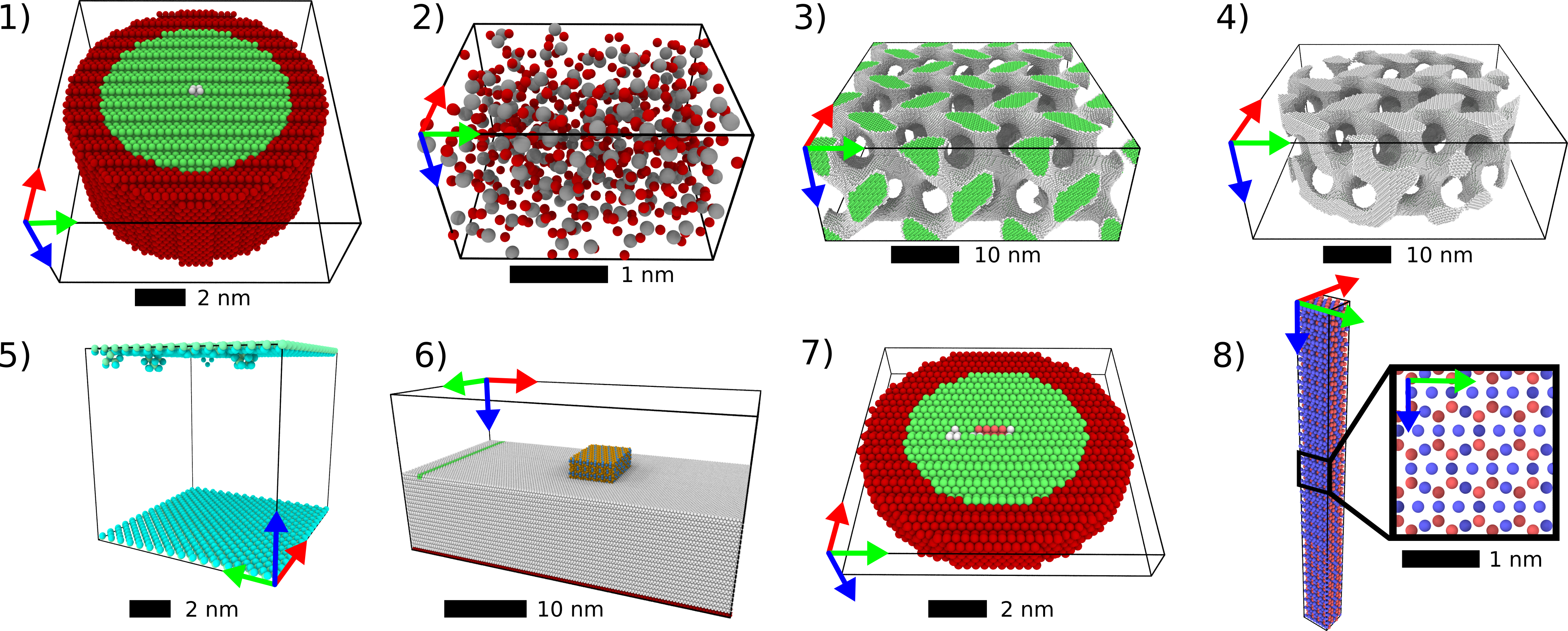
Figure 1: Snapshots of the atomistic samples used for the test simulations 1, 2, 3 4, 5, 6, 7 and 8. Color coding in (1,3,4, 7) is based on the common neighbor analysis [61]: green, fcc; light red, stacking fault; white, others; Color coding in (2,8) based on chemical species: grey, Si; dark-red, O; blue, Ca; light-red, Mg. Color coding in (5) based on diamond structure analyses [62]: turquoise, non-diamond atoms; atoms in diamond configuration are removed for clarity. Color coding in (6): light-grey, Mg hcp matrix atoms; green, fcc dislocation atoms. Within the cuboidale precipitate, orange and blue atoms are Mg and Al, respectively. Half of the Mg matrix atoms have been removed for clarity. In (1,7) dark-red colored atom are frozen. The simulation box axis x, y, z are represented by red, green, blue arrows, respectively. The scale bars indicate the dimension of each sample in nm.

1. Relaxation of a dislocation in Al: An edge dislocation [63] is inserted in an Al cylinder by displacing the atoms according to the anisotropic-elastic solution [64]. The cylinder has 25,340 atoms and a radius of 5.2 nm, including a border of width 1.4 nm where atoms are frozen in the $x$ and $y$ directions, see Fig. 1(1). Periodic boundary conditions (pbc) are used in the $z$-direction, with a box length of 5.0 nm. The eam potential by Mishin et al. is used [65].

2. Relaxation of a 6000K SiO₂ melt: The system consists of 648 atoms (216 Si and 432 O) within a simulation box of $2.0\times 2.6\times 1.6$ nm³ and pbc in all directions (Fig. 1(2)). The melt is obtained by md from an $\alpha$-quartz crystalline structure. Since this configuration is initially far from a $0$ K energy minimum, the maximum atomic displacement per step (dmax in lammps) had to be set to $0.001$ Å instead of $0.1$ Å (default value). This case uses the bks potential [58]. The long range coulombic interactions is calculated by a standard Ewald summation with an accuracy of $10^{-5}$ and a direct/reciprocal space cutoff of 1 nm.

3. Relaxation of bulk Au with a nano-porous gyroid structure: The structure has 613,035 atoms and is contained within a box of $44.6\times 42.6\times 15.7$ nm³ with full pbc. This case exhibits a particularly high surface over bulk ratio (21.4% of the atoms belong to surfaces) with complex curvatures, see Fig. 1(3). The ff is of the EAM type [66].

4. Relaxation of a Au nano-pillar with a nano-porous gyroid structure: This case is similar to case 3, but without pbc. The structure consists of 457,424 atoms and has a cylindrical shape with radius 42.6 nm and height 15.7 nm, see Fig. 1(4). It was cut out of the sample 3. 25.6% of atoms are surface atoms. Due to the absence of periodicity, only surface atoms (white) are visible in Fig. 1(4).

5. Relaxation of vacancies in Si: Five vacancies are distributed in a Si slab of 32,762 atoms contained in a box of $8.9^{3}$ nm³, see Fig. 1(5). The $x$ and $y$ directions are periodic. Si is simulated using the sw ff with the original parameterization in Ref. [51].

6. Relaxation of a dislocation in Mg with a precipitate: A Mg matrix contains an approximation of the isotropic displacement field of an edge dislocation on one side, and a relaxed Mg₁₇Al₁₂ precipitate on the other side. The Burgers vector of the dislocation is $b=a_{0}/3\hkl<-2110>$. The simulation box of $40\times 20\times 20$ nm³ contains 694,680 atoms and the precipitate has a cuboidal shape with dimensions of $5.5\times 7.8\times 6$ nm³, see Fig. 1(6). More details on this setup can be found elsewhere [67]. The meam potential from Kim et al. is used [68].

7. Energy barrier for vacancy migration in Al: neb is used to calculate the energy barrier for migration of a vacancy near an edge dislocation in Al. The setup is similar to 1, see Fig. 1(7). It consists of a cylinder of 7,010 atoms periodic in $z$ direction that contains a vacancy (surrounded by white atoms), and a relaxed edge dislocation with Burgers vector $1/2a\hkl<110>$ (light-red atoms). The cylinder has a length of 1.5 nm and a radius of 5.0 nm, including a border of width 1.4 nm where atoms are frozen in $x$ and $y$ directions (dark-red atoms). neb simulations are performed with 6 intermediate configurations, between 2 stable configurations that represent the hopping of the vacancy to a neighboring site. The ff is the same as in case 1.

8. Energy barrier of the synchroshear mechanism in Mg₂Ca: In brief, the synchroshear mechanism is responsible for the propagation of dislocations in the 0001 basal plane of the hcp Laves phase (Strukturbericht C14). It involves the synchronous glide of partial dislocations on adjacent basal planes. More details can be found elsewhere [69, 70, 50]. The system contains 5,376 atoms in a box of $2.5\times 2.1\times 28.0$ nm³. pbc are applied in all directions (See Fig. 1(8)). neb simulations are performed with 18 intermediate configurations as described elsewhere [50]. The ff is the meam from Kim et al. [49].

Case	Specificities	Atoms	ff	fire 2.0 performance
				vs cg	vs fire
1: dislocation in Al	Long range displacement field	25,340	EAM	1.2	29.3
2: melt of silicate glass	Electrostatic interactions and local disorder	648	BKS	$\infty$	$>3.0$
3: nano-porous bulk	Surface tension	613,035	EAM	$(1.5)$	$\infty$
4: nano-porous pillar	Surface tension and free boundaries	457,424	EAM	$(0.8)$	$\infty$
5: vacancies in silicon	3-body force field	32,762	SW	1.1	$>10.0$
6: dislocation-precipitate interaction	Configuration stability	694,680	MEAM	$\infty$	$\infty$
7: vacancy in Al	neb, simple path	7,010	EAM	–	1.8
8: synchroshear	neb, complex path	5,376	MEAM	–	2.9

Table 2: Test cases for the implementation of fire 2.0. The last two columns show the performance of fire 2.0 relative to cg or fire, i.e. the ratio of forces evaluation required for relaxation: cg/fire 2.0 or fire/fire 2.0. $\infty$ indicate that cg or fire are much too slow to relax the system, or not able at all. Values in brackets indicate that the relaxation with cg stopped before reaching the threshold (line search alpha is zero) but can still be considered as relaxed.

5.4 Results and discussion

The computationally most expensive task in atomistic simulations is typically the calculation of the interatomic forces, therefore the number of force evaluations is used for comparing minimizer performances. Except otherwise mentioned, the threshold f2norm used in this work is $=10^{-8}$eV/Å. The evolution of f2norm as a function of the number of force evaluations is shown in Fig. 1. Tab. 2 indicates the increase in performance obtained by fire 2.0 versus cg and fire. The performance in optimizing a configuration is determined by the ratio of the number of forces evaluations required by cg or fire to reach the threshold, over the number of forces evaluations required by fire 2.0. A comparison with l-bfgs is outside the scope of this work which is based on lammps, where l-bfgs is not included. A recent comparison between a fire-based algorithm and l-bfgs was reported by Shuang et al. [31].

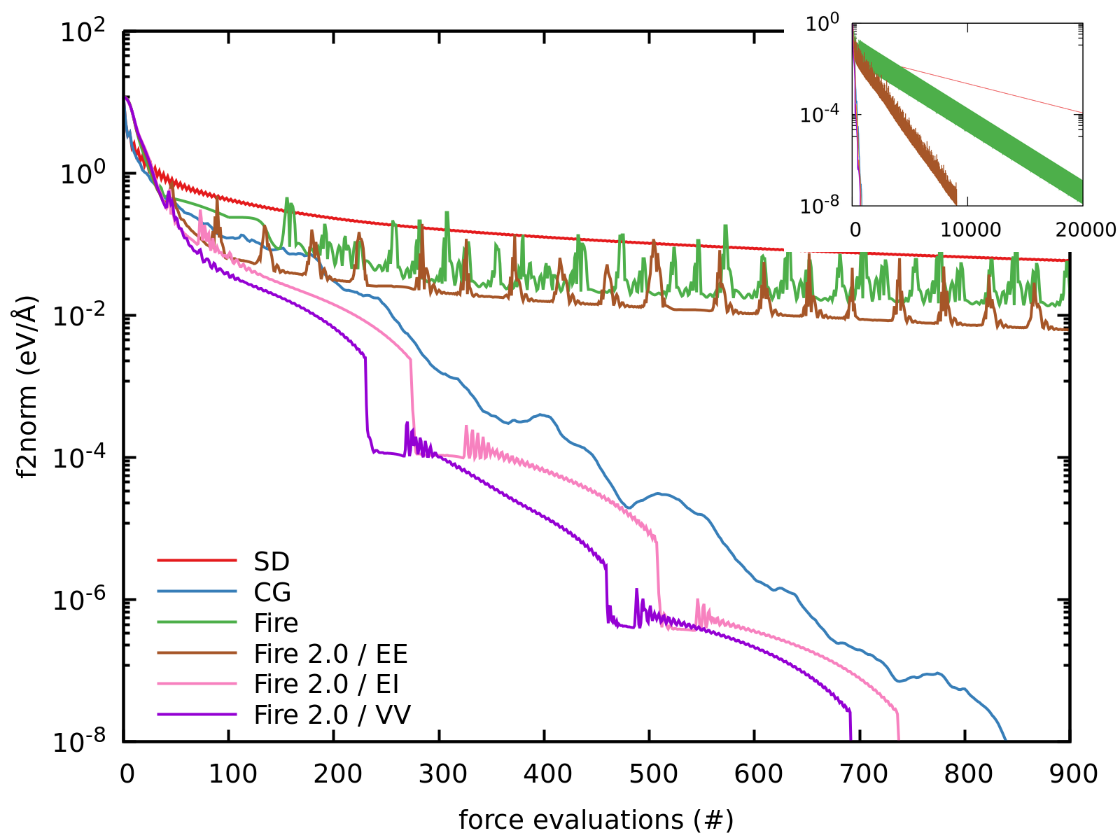
(1) Dislocation in aluminum.

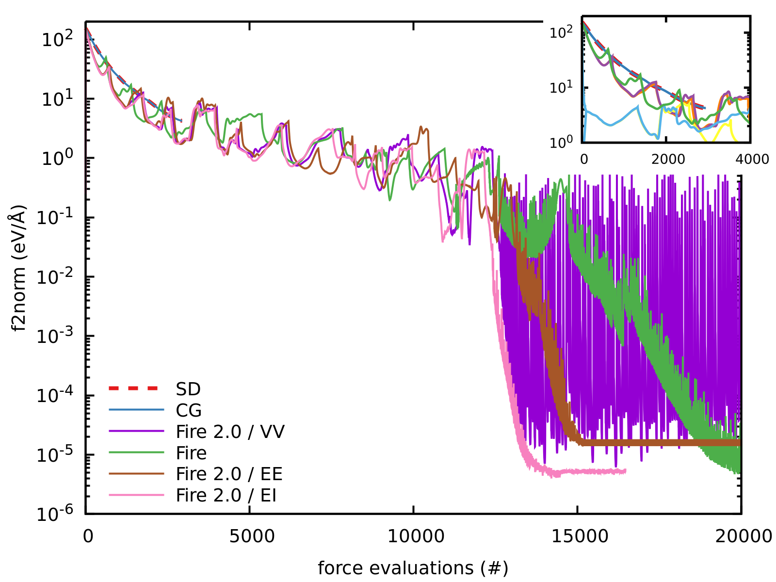
(2) Silica melt.

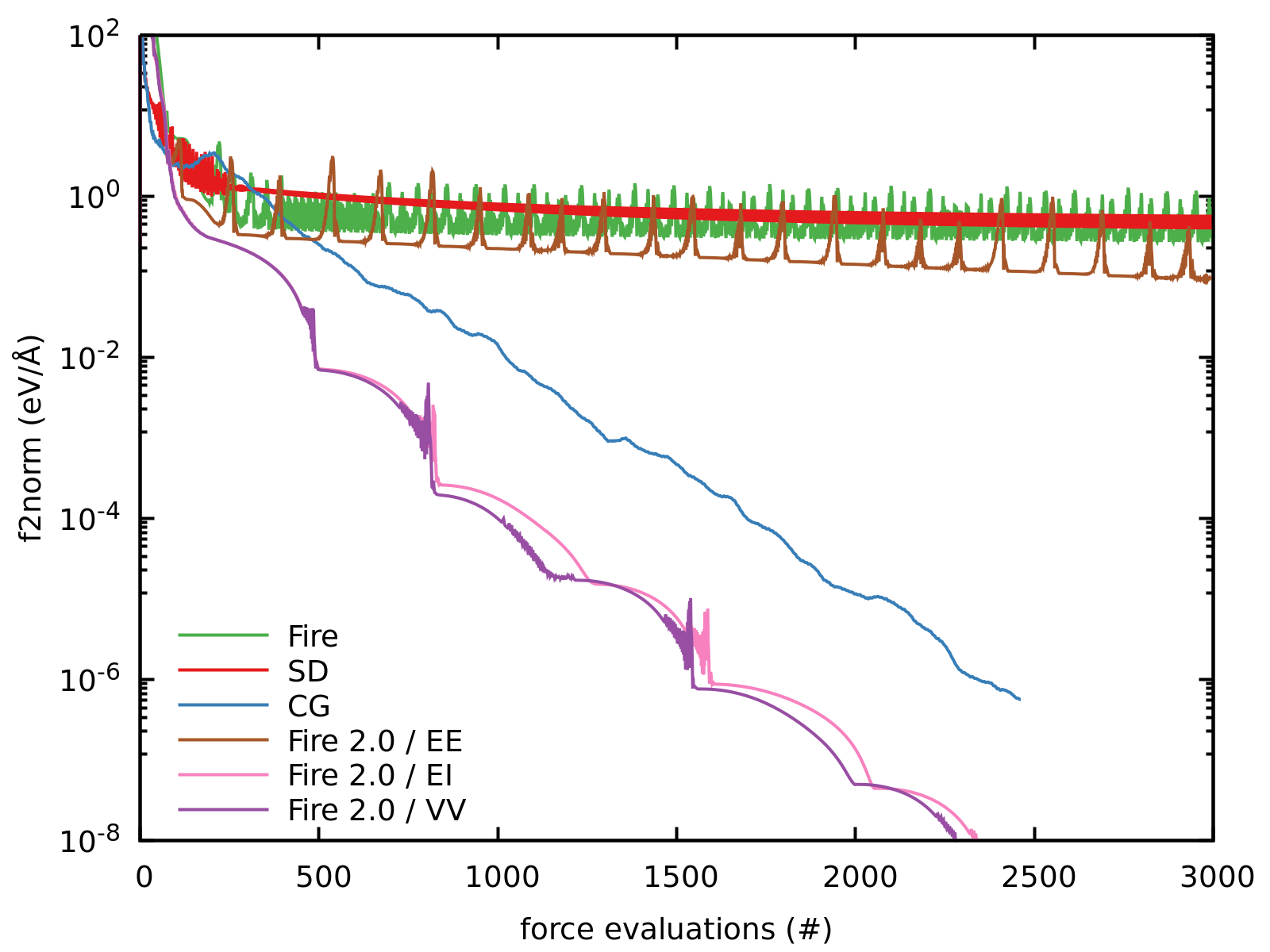
(3) Nano-porous gold, bulk.

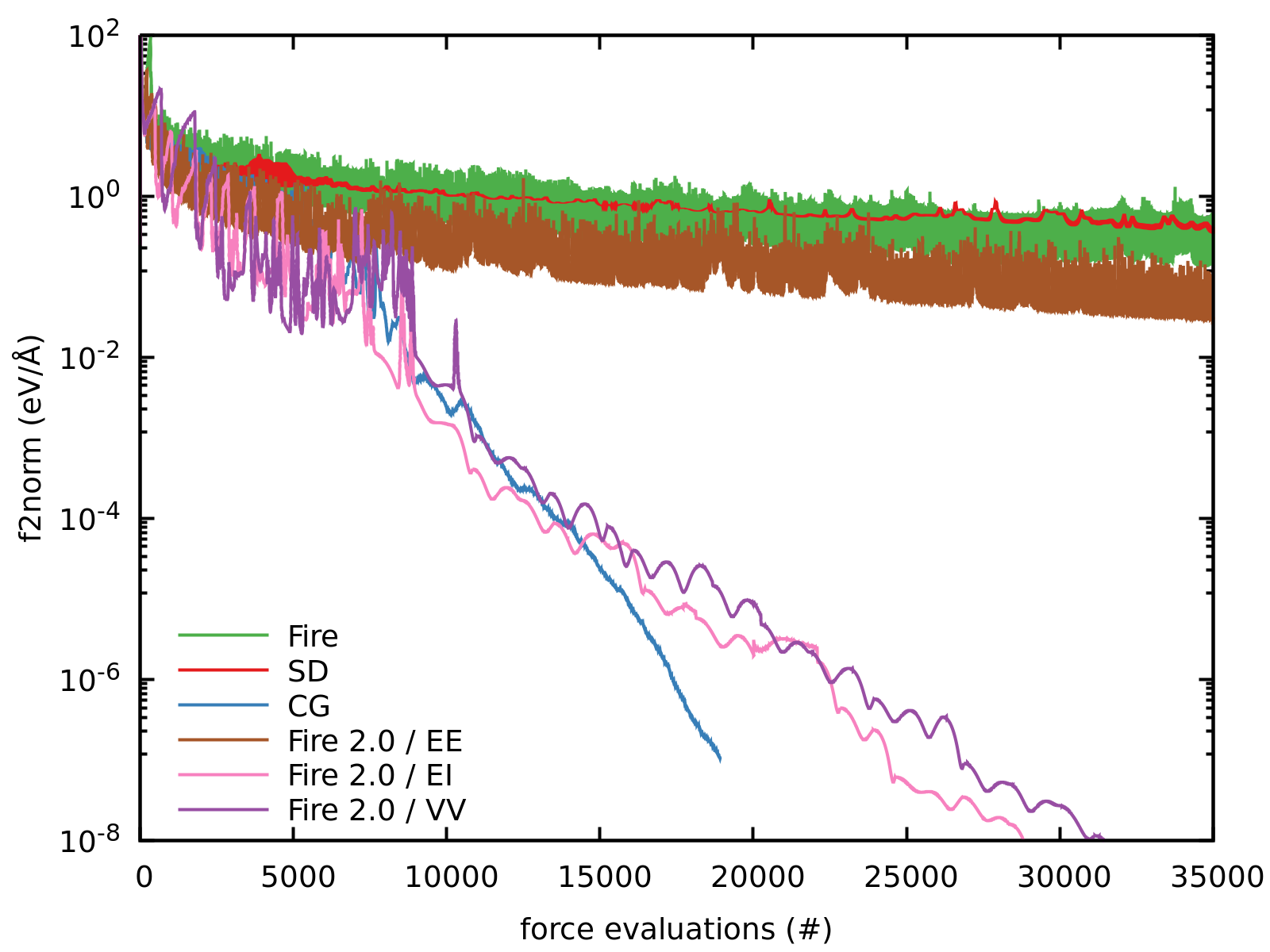
(4) Nano-porous gold, pillar.

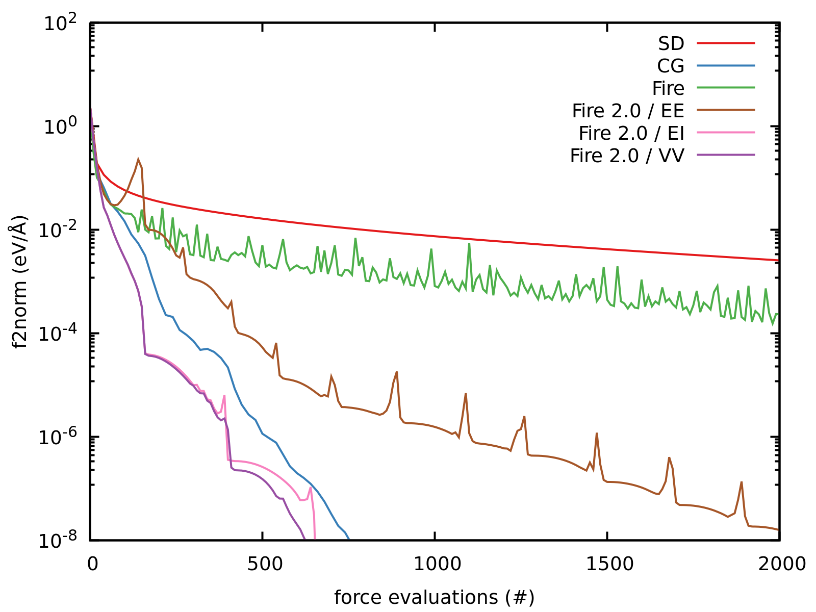
(5) Silicon vacancies.

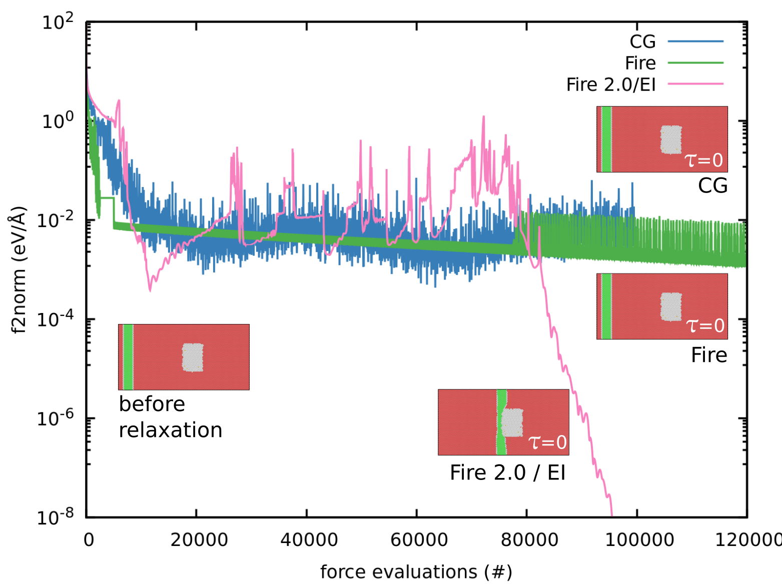
(6) Dislocation and precipitate in Mg alloys.

Figure 2: Force f2norm as a function of the number of interatomic forces evaluation during minimization. Subfigures 1 to 6 correspond to the test cases 1 to 6, respectively. (Continue on next page.)

Figure 2: (Continued) The color of curves indicates the minimization method: steepest descent (sd, red line), conjugate gradient (cg, blue line), fire (Fire, green line). For fire 2.0, the color indicates the time integration scheme: Euler Explicit (EE, brown line), Euler Semi-implicit (EI, pink line) and Velocity-Verlet (VV, purple line). Insets in 2(6) represent the minimized configurations for different minimization methods, with atoms colored according to the common neighbors analysis method (red, Mg HCP; green, Mg FCC and dislocation; grey, Mg₁₇Al₁₂ precipitate).

5.4.1 cg vs fire 2.0

fire 2.0 performs better than cg in the two simple cases 5 and 1, with a ratio of $1.1\times$ and $1.2\times$, respectively. The relaxation of the long range ff in the case 2 is not possible using cg, which terminates with the lammps’s stopping criterion linesearch alpha is zero at comparatively large f2norm. Generally, this occurs when no minimum can be found by line search, for example when the backtracking algorithm backtracks all the way to the initial point. A similar behavior is seen in test case 6: cg fails to reduce the forces sufficiently. Note that the output configuration is clearly different to the one obtained with fire 2.0, see the insets in Fig. 2(6). Similarly to fire, cg predicts that the dislocation remains in the Mg matrix far away from the precipitate, whereas fire 2.0 predicts that the dislocation moves towards the precipitate.

In test cases 3 and 4 (nano-porous Au) cg fails to reach the strict f2norm threshold of $10^{-8}$eV/Å, see Figs. 2(3) and 2(4). Line search fails when f2norm is below $10^{-6}$eV/Å. To quantify the performance of fire 2.0, we thus compare the number of force evaluations requires to reach the lowest f2norm achieved by cg. Here, fire 2.0 performs better than cg in problem 3 (bulk), but worse in 4 (free boundaries).

5.4.2 fire vs fire 2.0

fire 2.0 performs better than fire as implemented in lammps in all the test cases. The smallest speedups of $1.8\times$ and $2.9\times$ are seen in the neb calculations of problems 7 and 8, respectively. A larger speedup of more than $3\times$ is obtained in case 2, where the bks potential is used. Note that it is particularly difficult to relax the long-range coulombic interaction, so that the desired force stopping criterion was not reached. The relaxation with fire 2.0 stopped when f2norm reached a plateau, see Fig. 2(2). In this plateau region, fire 2.0 detected repeated attempts at uphill motion ($P(t)<0$), and so minimization was terminated with return value MAXVDOTF. A speedup can still be defined by comparing the number of force evaluations at which fire reaches a f2norm similar to the one at the end of the fire 2.0 minimization. Much larger speedups of $10\times$ and $30\times$ are obtained in the cases 5 and 1, respectively. Finally, in the cases 3, 4 and 6 convergence of fire is so slow that the desired f2norm threshold is not reached.

5.4.3 fire 2.0: Influence of the time integration scheme

Fig. 2 shows the minimization of the problems 1 to 6 with fire 2.0 and the four integration schemes. With an Euler Explicit scheme, fire 2.0 shows a similar poor performance as sd and fire. Switching to Euler Implicit integration improves the performance significantly. With this integrator, fire 2.0 typically outperforms cg in all these cases. The Velocity Verlet integrator, on the other hand, performs slightly better than the others in problems 1, 3 and 5, but not in problems 2 and 4. In particular, the case 2 (Fig. 2(2)) has stability issues.

As for the cases 1 to 6, the neb cases 7 and 8 show a similar poor performance as fire while using fire 2.0 with an Euler Explicit scheme. By switching to Euler Implicit integration, as before, fire 2.0 typically outperforms fire. The Velocity Verlet integrator exhibits mixed behavior: it performs better than the other integrators in problem 7 but not in problem 8, the latter having stability issues.

5.4.4 fire 2.0: Influence of individual parameters

We have investigated the influence of the parameters $\alpha_{start}$ and $\Delta t_{max}$ on the performance of fire 2.0. Since the observed trends do not depend on the problem, the computationally less expensive problem 5 has been chosen for this parameter study. Note that $\alpha_{start}$ and $\Delta t_{max}$ are controlled by the lammps parameters alpha0 and tmax, respectively.

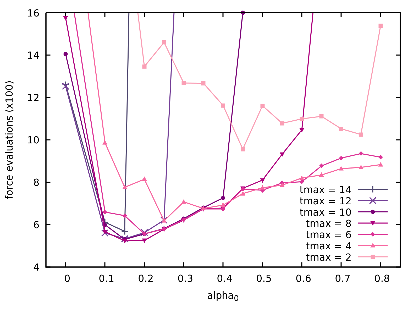
(1)

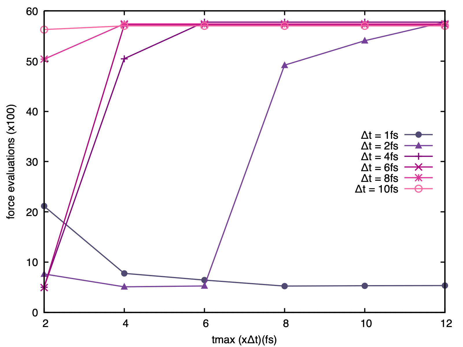
(2)

Figure 3: Influence of the parameters alpha0 (1) and tmax (2) on the minimization performances, characterized by the number of force evaluations required to reach the force threshold in the case 5. (1) shows the performance as a function of alpha0 for different choice of tmax, with $\Delta$t = 1fs. (2) shows the performance as a function of tmax for different choice of timestep $\Delta$t, with alpha0 = 0.15.

The performance as a function of $\alpha_{start}$ for different choice of $\Delta t_{max}$ ($\Delta t=1$ps) are shown on Fig. 3(1). As seen on Fig. 3(1), best values lie in a range from 0.10 to 0.25. Increasing $\alpha_{start}$ does not improve performance. For $\Delta t_{max}>6$ps, it even leads to dramatic performance reduction. Generally, large values of tmax will benefit from lower values of alpha0, around 0.10 – 0.15.

The performances as a function of $\Delta t_{max}$ for different choice of $\Delta t$ ($\alpha_{start}=0.15$) is shown on Fig. 3(2). The maximum value for the timestep $\Delta t_{max}$ is controlled by the coefficient tmax applied on the timestep $\Delta t$. That is $\Delta t_{max}=\texttt{tmax}*\texttt{timestep}$. As seen on Fig. 3(2), the performances largely depend on the correlated choice of the timestep and tmax. The optimum $\Delta t$ for running dynamics simulation in such system being $1\text{\,}\mathrm{fs}$, it appears that choosing $\Delta t$ at least 4 times bigger is not relevant and leads to poor performances. In this case, fire 2.0 shows good performance for $\Delta t_{max}<$12\text{\,}\mathrm{fs}$$, which correspond to tmax from 6 to 12, depending on the timestep. Generally, one can consider reducing tmax to improve the stability of the minimization.

5.4.5 fire 2.0: Nudged elastic band method

fire 2.0 is $1.8$ and $2.9$ times faster than fire in the cases 7 and 8, respectively, see Tab. 2. Note that case 8, where the relative performance of fire 2.0 is better, is also the more complex case (complex mechanism and more images). Finally, a comparison of fire 2.0 and cg is not possible in these cases, because neb calculations in lammps require damped dynamics minimizers.

5.4.6 fire 2.0: On the usage of preconditioners

For geometrical optimization of atomistic configurations, preconditioners are known to largely enhanced the efficiency of the algorithms by considering known characteristics of the system, like the local atomic neighborhood [71]. For more details on preconditioners and how to determine them, the reader should refer to the recent work of Packwood et al. [72]. Preconditioners are especially efficient on large systems and could then reduce the difference we observe between cg and fire 2.0. With a similar goal as the preconditioner, that is the reduction of degrees of freedom to be optimized, we also investigated the influence of a pre-relaxation with a different minimizer on the performance of fire 2.0. This pre-relaxation was performed with the quickmin minimizer for 100 iterations, as implemented in lammps [7]. In all the problems but one, we did not observe any gain. Only the case 2 with long range atomic interactions evidence a significant advantage of performing this pre-relaxation, with a speedup close to 30%. That also improved the stability of fire 2.0 with Velocity-Verlet for the same problem.

5.5 General aspects

fire 2.0 minimizes faster than fire and can potentially reach lower residual forces. In the case of neb simulations, the performance gain increases with the complexity of the setup. When comparing to cg, fire 2.0 shows better performance except in case 4, the non-periodic nanoporous Au structure (Fig. 2(4)). Recall that the system was created by cutting bulk nanoporous Au (case 3) and removing pbc. The structure thus undergoes a sudden global shrinkage at the beginning of the minimization, which can easily be optimized by cg. In contrast, pseudo-dynamics relaxators like fire and fire 2.0 are sensitive to such scaling by generating a shock wave that has to be damped during optimization and thus may hamper minimization. In the bulk case (case 3), where there is no such global dynamic effect, fire 2.0 performs better than cg, which also indicates that the algorithm remains robust with a large amount of free surfaces. On all other systems, fire 2.0 shows various levels performance increase in comparison to cg, between 20% and 3000%. In addition, cg is not able to minimize the forces in some cases, due either to the long range stress field (case 6) or long range atomic interactions (case 2).

cg sometimes terminates prematurely (at a high level of residual force), because line search fails. Similarly, fire or fire 2.0 could terminate prematurely if convergence is slow and the chosen maximum number of force evaluations is too low. The resulting structure is then insufficiently optimized. Here, this was seen in case 6 (Fig. 2(6)), where fire and cg yield a different dislocation position than fire 2.0. The latter is less susceptible to premature termination, because it does not suffer from line search problems and typically minimizes with fewer number of force evaluations. As a general statement, we note that reaching low f2norm values is crucial and analyzing an insufficiently relaxed structure could lead to wrong interpretations. This is especially important in statics and quasi-statics calculations of critical stresses. As a good practice, we suggest to always indicate the exact f2norm value alongside results in published work.

Among all the parameters that affect the behavior and performance of fire 2.0, the time integration scheme is the most important. Overall, as presented in the results above, Euler Implicit integrator provides robust minimizations at the cost of a slightly reduce performance. Hence we recommend the usage of fire 2.0 with an Euler Implicit integrator. Similarly, the very recent work of Shuang et al. [31] also recommended to couple the fire approach with a semi-implicit Euler integrator.

More generally, Tab. 1 list the parametrization of fire 2.0 accessible by the command min_modify as implemented in lammps and the associated default values we recommend to use. More specifically, tmax can be reduced to improve the stability but should range from $2$ to $12$, and alpha0 should range from $0.10$ to $0.25$. In any case, we recommend to set the simulation timestep (command timestep in lammps) to the same value as in MD at low temperature.

6 Summary

In this work we describe fire 2.0, an optimized version of the fire minimization algorithm within the lammps molecular dynamics simulator, and add important details to the canonical publication [17]. The choice of time integration scheme has appeared to be crucial for fire and is now clearly discussed. A non-symplectic scheme like Euler explicit should not be used. We have shown the clear advantages of fire 2.0 versus fire and versus conjugate gradient through several examples in materials science: fire 2.0 is significantly faster than fire or conjugate gradient and can result in lower energy structures not found by other algorithms.

We intend fire 2.0 to entirely replace fire, the present work being a complement of the original publication [17]. Ultimately, this work intends to provide insights on performing more accurate and more efficient forces minimization of atomistic systems.

Data availability

The source code of the implementation of fire 2.0 in lammps is freely available online, as described in B. The raw data required to reproduce the findings presented in this paper cannot be shared at this time as the data also forms part of an ongoing study.

Appendix A Integration in fire 2.0

Algorithm 3 Explicit Euler integration in fire 2.0

1:$\mathbf{v}(t)\leftarrow(1-\alpha)\cdot\mathbf{v}(t)+\alpha\mathbf{F}(\mathbf{x}(t))\cdot|\mathbf{v}(t)|/|\mathbf{F}(\mathbf{x}(t))|$ $\triangleright$ Mixing

2:$\mathbf{x}(t+\Delta t)\leftarrow\mathbf{x}(t)+\Delta t\cdot\mathbf{v}(t)$

3:$\mathbf{v}(t+\Delta t)\leftarrow\mathbf{v}(t)+\Delta t\cdot\mathbf{F}(\mathbf{x}(t+\Delta t))/m$

4:Calculate $E(x(t+\Delta t))$

5:$\mathbf{F}(\mathbf{x}(t+\Delta t))\leftarrow-\vec{\nabla}E(\mathbf{x}(t+\Delta t))$

Algorithm 4 Semi-implicit Euler integration in fire 2.0

1:$\mathbf{v}(t+\Delta t)\leftarrow\mathbf{v}(t)+\Delta t\cdot\mathbf{F}(\mathbf{x}(t))/m$

2:$\mathbf{v}(t+\Delta t)\leftarrow(1-\alpha)\cdot\mathbf{v}(t)+\alpha\mathbf{F}(\mathbf{x}(t))\cdot|\mathbf{v}(t)|/|\mathbf{F}(\mathbf{x}(t))|$ $\triangleright$ Mixing

3:$\mathbf{x}(t+\Delta t)\leftarrow\mathbf{x}(t)+\Delta t\cdot\mathbf{v}(t+\Delta t)$

4:Calculate $E(x(t+\Delta t))$

5:$\mathbf{F}(\mathbf{x}(t+\Delta t))\leftarrow-\vec{\nabla}E(\mathbf{x}(t+\Delta t))$

Algorithm 5 Leapfrog integration in fire 2.0

1:$\mathbf{v}(-\nicefrac{{1}}{{2}}\Delta t)\leftarrow-\nicefrac{{1}}{{2}}\Delta t\cdot\mathbf{F}(\mathbf{x}(t))/m$ $\triangleright$ Initialization

2:$\mathbf{v}(t+\nicefrac{{1}}{{2}}\Delta t)\leftarrow\mathbf{v}(t-\nicefrac{{1}}{{2}}\Delta t)+\Delta t\cdot\mathbf{F}(\mathbf{x}(t))/m$

3:$\mathbf{v}(t+\nicefrac{{1}}{{2}}\Delta t)\leftarrow(1-\alpha)\cdot\mathbf{v}(t+\nicefrac{{1}}{{2}}\Delta t)+\alpha\mathbf{F}(\mathbf{x}(t))\cdot|\mathbf{v}(t+\nicefrac{{1}}{{2}}\Delta t)|/|\mathbf{F}(\mathbf{x}(t))|$ $\triangleright$ Mixing

4:$\mathbf{x}(t+\Delta t)\leftarrow\mathbf{x}(t)+\Delta t\cdot\mathbf{v}(t+\nicefrac{{1}}{{2}}\Delta t)$

5:Calculate $E(x(t+\Delta t))$

6:$\mathbf{F}(\mathbf{x}(t+\Delta t))\leftarrow-\vec{\nabla}E(\mathbf{x}(t+\Delta t))$

Algorithm 6 Velocity Verlet integration in fire 2.0

1:$\mathbf{v}(t+\nicefrac{{1}}{{2}}\Delta t)\leftarrow\mathbf{v}(t)+\nicefrac{{1}}{{2}}\Delta t\cdot\mathbf{F}(\mathbf{x}(t))/m$

2:$\mathbf{v}(t+\nicefrac{{1}}{{2}}\Delta t)\leftarrow(1-\alpha)\cdot\mathbf{v}(t+\nicefrac{{1}}{{2}}\Delta t)+\alpha\mathbf{F}(\mathbf{x}(t))\cdot|\mathbf{v}(t+\nicefrac{{1}}{{2}}\Delta t)|/|\mathbf{F}(\mathbf{x}(t))|$ $\triangleright$ Mixing

3:$\mathbf{x}(t+\Delta t)\leftarrow\mathbf{x}(t)+\Delta t\cdot\mathbf{v}(t+\nicefrac{{1}}{{2}}\Delta t)$

4:Calculate $E(x(t+\Delta t))$

5:$\mathbf{F}(\mathbf{x}(t+\Delta t))\leftarrow-\vec{\nabla}E(\mathbf{x}(t+\Delta t))$

6:$\mathbf{v}(t+\Delta t)\leftarrow\mathbf{v}(t+\nicefrac{{1}}{{2}}\Delta t)+\nicefrac{{1}}{{2}}\Delta t\cdot\mathbf{F}(\mathbf{x}(t+\Delta t))/m$

Appendix B Source code of fire 2.0

fire 2.0 is currently being pulled in the master branch of lammps (https://github.com/lammps/lammps/pull/1052) and should replace the current implementation of fire. Please refer to the documentation of lammps for the most up-to-date indications.

The development version of the source code is available as a fork of lammps. It can be found in the GitHub repository of JG, branch adaptglok (https://github.com/jguenole/lammps/tree/adaptglok). The latest commit to the date of this manuscript is 426ca97 (https://github.com/lammps/lammps/pull/1052/commits/426ca97aa6ecf289f824a70781f3640d429e6ab3).

References

- [1] R. Fletcher, Practical Methods of Optimization, 2nd Edition, John Wiley & Sons, 2013 (2013). doi:10.1002/9781118723203.
- [2] J. Nocedal, S. J. Wright, Numerical Optimization, 2nd Edition, Springer, 2006 (2006).
- [3] T. Schlick, Molecular modeling and simulation: an interdisciplinary guide, Vol. 21, Springer, 2010 (2010).
- [4] Y. Umeno, T. Shimada, T. Kitamura, Dislocation nucleation in a thin cu film from molecular dynamics simulations: Instability activation by thermal fluctuations, Physical Review B 82 (10) (sep 2010). doi:10.1103/physrevb.82.104108.
- [5] E. Bitzek, P. Gumbsch, Dynamic aspects of dislocation motion: Atomistic simulations, Mater. Sci. Eng. A 400-401 (2005) 40–44 (2005). doi:10.1016/j.msea.2005.03.047.
- [6] J. J. Möller, E. Bitzek, Fracture toughness and bond trapping of grain boundary cracks, Acta Mater. 73 (2014) 1–11 (2014). doi:10.1016/j.actamat.2014.03.035.
- [7] D. Sheppard, R. Terrell, G. Henkelman, Optimization methods for finding minimum energy paths, The Journal of Chemical Physics 128 (13) (2008). doi:10.1063/1.2841941.
- [8] D. Perez, B. P. Uberuaga, Y. Shim, J. G. Amar, A. F. Voter, Accelerated molecular dynamics methods: introduction and recent developments, Annu. Rep. Comput. Chem. 5 (2009) 79–98 (2009).
- [9] S. Plimpton, Fast parallel algorithms for short-range molecular dynamics, Journal of Computational Physics 117 (1995) 1–19 (1995). doi:10.1006/jcph.1995.1039.
-
[10]
M. J. Abraham, T. Murtola, R. Schulz, S. Páll, J. C. Smith, B. Hess,
E. Lindahl,
Gromacs:
High performance molecular simulations through multi-level parallelism from
laptops to supercomputers, SoftwareX 1-2 (2015) 19 – 25 (2015).
doi:https://doi.org/10.1016/j.softx.2015.06.001.
URL http://www.sciencedirect.com/science/article/pii/S2352711015000059 -
[11]
J. Stadler, R. Mikulla, H.-R. Trebin,
Imd: A software package for
molecular dynamics studies on parallel computers, International Journal of
Modern Physics C 08 (05) (1997) 1131–1140 (1997).
doi:10.1142/S0129183197000990.
URL https://doi.org/10.1142/S0129183197000990 -
[12]
W. Smith, C. Yong, P. Rodger,
Dl_poly: Application to
molecular simulation, Molecular Simulation 28 (5) (2002) 385–471 (2002).
doi:10.1080/08927020290018769.
URL https://doi.org/10.1080/08927020290018769 - [13] S. T. Chill, M. Welborn, R. Terrell, L. Zhang, J. C. Berthet, A. Pedersen, H. Jónsson, G. Henkelman, EON: Software for long time simulations of atomic scale systems, Model. Simul. Mater. Sci. Eng. 22 (5) (2014). arXiv:arXiv:1408.1149, doi:10.1088/0965-0393/22/5/055002.
- [14] J. Blomqvist, M. Dulak, J. Friis, C. Hargus, The Atomic Simulation Environment — A Python library for working with atoms, J. Phys. Condens. Matter 29 (March) (2017) 273002 (2017). doi:10.1088/1361-648X/aa680e.
- [15] J. J.R. Beeler, Radiation Effects Computer Experiments, Defects in Crystalline Solids, North-Holland, 1983 (1983).
-
[16]
D. Sheppard, R. Terrell, G. Henkelman,
Optimization methods for finding
minimum energy paths, The Journal of Chemical Physics 128 (13) (2008) 134106
(2008).
doi:10.1063/1.2841941.
URL https://doi.org/10.1063/1.2841941 - [17] E. Bitzek, P. Koskinen, F. Gähler, M. Moseler, P. Gumbsch, Structural relaxation made simple, Physical Review Letters 97 (2006) 170201 (Oct. 2006). doi:10.1103/PhysRevLett.97.170201.
-
[18]
T. Nogaret, W. A. Curtin, J. A. Yasi, L. G. Hector, D. R. Trinkle,
Atomistic study of
edge and screw (c + a) dislocations in magnesium, Acta Mater. 58 (13)
(2010) 4332–4333 (2010).
doi:10.1016/j.actamat.2010.04.022.
URL http://dx.doi.org/10.1016/j.actamat.2010.04.022 -
[19]
L. Pastewka, A. Klemenz, P. Gumbsch, M. Moseler,
Screened empirical
bond-order potentials for si-c, Phys. Rev. B 87 (2013) 205410 (May 2013).
doi:10.1103/PhysRevB.87.205410.
URL https://link.aps.org/doi/10.1103/PhysRevB.87.205410 - [20] R. A. Riggleman, J. F. Douglas, J. J. De Pablo, Antiplasticization and the elastic properties of glass-forming polymer liquids, Soft Matter 6 (2) (2010) 292–304 (2010). doi:10.1039/b915592a.
- [21] M. Amsler, J. A. Flores-Livas, L. Lehtovaara, F. Balima, S. A. Ghasemi, D. MacHon, S. Pailhès, A. Willand, D. Caliste, S. Botti, A. San Miguel, S. Goedecker, M. A. Marques, Crystal structure of cold compressed graphite, Phys. Rev. Lett. 108 (6) (2012) 1–4 (2012). arXiv:1109.1158, doi:10.1103/PhysRevLett.108.065501.
-
[22]
S. Singh, M. D. Ediger, J. J. De Pablo,
Ultrastable glasses from in silico
vapour deposition, Nat. Mater. 12 (2) (2013) 139–144 (2013).
doi:10.1038/nmat3521.
URL http://dx.doi.org/10.1038/nmat3521 - [23] S. Dagois-Bohy, B. P. Tighe, J. Simon, S. Henkes, M. Van Hecke, Soft-sphere packings at finite pressure but unstable to shear, Phys. Rev. Lett. 109 (9) (2012) 1–5 (2012). arXiv:1203.3364, doi:10.1103/PhysRevLett.109.095703.
- [24] R. Y. Brogaard, R. Henry, Y. Schuurman, A. J. Medford, P. G. Moses, P. Beato, S. Svelle, J. K. Nørskov, U. Olsbye, Methanol-to-hydrocarbons conversion: The alkene methylation pathway, J. Catal. 314 (2014) (2014) 159–169 (2014). doi:10.1016/j.jcat.2014.04.006.
- [25] J. Fanfrlík, A. K. Bronowska, J. Řezáč, O. Přenosil, J. Konvalinka, P. Hobza, A reliable docking/scoring scheme based on the semiempirical quantum mechanical PM6-DH2 method accurately covering dispersion and H-bonding: HIV-1 protease with 22 ligands, J. Phys. Chem. B 114 (39) (2010) 12666–12678 (2010). doi:10.1021/jp1032965.
- [26] D. Asenjo, J. D. Stevenson, D. J. Wales, D. Frenkel, Visualizing basins of attraction for different minimization algorithms, J. Phys. Chem. B 117 (42) (2013) 12717–12723 (2013). arXiv:1309.7845, doi:10.1021/jp312457a.
- [27] E. MacHado-Charry, L. K. Béland, D. Caliste, L. Genovese, T. Deutsch, N. Mousseau, P. Pochet, Optimized energy landscape exploration using the ab initio based activation-relaxation technique, J. Chem. Phys. 135 (3) (2011). doi:10.1063/1.3609924.
- [28] A. Cromer, Stable solutions using the euler approximation, American Journal of Physics 49 (5) (1981) 455–459 (1981).
- [29] L. Verlet, Computer ”experiments” on classical fluids. i. thermodynamical properties of lennard-jones molecules, Physical Review 159 (1) (1967) 98 (Jul. 1967). doi:10.1103/PhysRev.159.98.
-
[30]
D. Donnelly, E. Rogers, Symplectic
integrators: An introduction, American Journal of Physics 73 (10) (2005)
938–945 (2005).
arXiv:https://doi.org/10.1119/1.2034523, doi:10.1119/1.2034523.
URL https://doi.org/10.1119/1.2034523 - [31] F. Shuang, P. Xiao, R. Shi, F. Ke, Y. Bai, Influence of integration formulations on the performance of the fast inertial relaxation engine (FIRE) method, Computational Materials Science 156 (2019) 135–141 (jan 2019). doi:10.1016/j.commatsci.2018.09.049.
- [32] J. Stadler, R. Mikulla, H.-R. Trebin, Imd: A software package for molecular dynamics studies on parallel computers, International Journal of Modern Physics C 08 (05) (1997) 1131–1140 (1997). arXiv:http://www.worldscientific.com/doi/pdf/10.1142/S0129183197000990, doi:10.1142/S0129183197000990.
- [33] E. B. Tadmor, R. E. Miller, Modeling Materials: Continuum, Atomistic and Multiscale Techniques, Cambridge University Press, 2011 (2011). doi:10.1017/CBO9781139003582.
- [34] M. S. Daw, M. I. Baskes, Embedded-atom method: Derivation and application to impurities, surfaces, and other defects in metals, Physical Review B 29 (1984) 6443–6453 (Jun. 1984). doi:10.1103/PhysRevB.29.6443.
- [35] S. M. Foiles, M. I. Baskes, M. S. Daw, Embedded-atom-method functions for the fcc metals cu, ag, au, ni, pd, pt, and their alloys, Physical Review B 33 (1986) 7983–7991 (Jun. 1986). doi:10.1103/PhysRevB.33.7983.
- [36] D. Rodney, G. Martin, Dislocation pinning by glissile interstitial loops in a nickel crystal: A molecular-dynamics study, Physical Review B 61 (2000) 8714–8725 (Apr. 2000). doi:10.1103/PhysRevB.61.8714.
-
[37]
D. Bachurin, D. Weygand, P. Gumbsch,
Dislocation–grain
boundary interaction in ¡111¿ textured thin metal films, Acta Materialia
58 (16) (2010) 5232–5241 (2010).
doi:10.1016/j.actamat.2010.05.037.
URL http://www.sciencedirect.com/science/article/pii/S1359645410003228 -
[38]
A. Prakash, J. Guénolé, J. Wang, J. Müller, E. Spiecker, M. Mills,
I. Povstugar, P. Choi, D. Raabe, E. Bitzek,
Atom
probe informed simulations of dislocation–precipitate interactions reveal
the importance of local interface curvature, Acta Materialia 92 (0) (2015)
33–45 (2015).
doi:10.1016/j.actamat.2015.03.050.
URL http://www.sciencedirect.com/science/article/pii/S1359645415002268 - [39] A. Prakash, E. Bitzek, Idealized vs. realistic microstructures: An atomistic simulation case study on gamma / gamma prime microstructures, Materials 10 (1) (2017) 88 (jan 2017). doi:10.3390/ma10010088.
- [40] A. Prakash, D. Weygand, E. Bitzek, Influence of grain boundary structure and topology on the plastic deformation of nanocrystalline aluminum as studied by atomistic simulations, International Journal of Plasticity 97 (2017) 107–125 (oct 2017). doi:10.1016/j.ijplas.2017.05.011.
- [41] L. A. Zepeda-Ruiz, A. Stukowski, T. Oppelstrup, V. V. Bulatov, Probing the limits of metal plasticity with molecular dynamics simulations, Nature 550 (7677) (2017) 492–495 (2017). doi:10.1038/nature23472.
- [42] Y. Chang, W. Lu, J. Guénolé, L. T. Stephenson, A. Szczpaniak, P. Kontis, A. K. Ackerman, F. F. Dear, I. Mouton, X. Zhong, S. Zhang, D. Dye, C. H. Liebscher, D. Ponge, S. Korte-Kerzel, D. Raabe, B. Gault, Ti and its alloys as examples of cryogenic focused ion beam milling of environmentally-sensitive materials, Nature Communications 10 (1) (feb 2019). doi:10.1038/s41467-019-08752-7.
- [43] M. I. Baskes, Application of the embedded-atom method to covalent materials: A semiempirical potential for silicon, Physical Review Letters 59 (1987) 2666–2669 (Dec. 1987). doi:10.1103/PhysRevLett.59.2666.
- [44] M. I. Baskes, J. S. Nelson, A. F. Wright, Semiempirical modified embedded-atom potentials for silicon and germanium, Physical Review B 40 (9) (1989) 6085–6100 (Sep. 1989). doi:10.1103/PhysRevB.40.6085.
- [45] M. I. Baskes, Modified embedded-atom potentials for cubic materials and impurities, Physical Review B 46 (5) (1992) 2727–2742 (Aug. 1992). doi:10.1103/PhysRevB.46.2727.
- [46] B.-J. Lee, M. Baskes, Second nearest-neighbor modified embedded-atom-method potential, Physical Review B 62 (13) (2000) 8564 (2000). doi:10.1103/physrevb.62.8564.
-
[47]
B.-J. Lee,
A
modified embedded atom method interatomic potential for silicon, Calphad -
Computer Coupling of Phase Diagrams and Thermochemistry 31 (1) (2007) 95–104
(2007).
doi:10.1016/j.calphad.2006.10.002.
URL http://www.sciencedirect.com/science/article/B6TWC-4M942BN-1/2/e55938f902b03522a1bfabb6f4926aec - [48] B. Jelinek, S. Groh, M. F. Horstemeyer, J. Houze, S. G. Kim, G. J. Wagner, A. Moitra, M. I. Baskes, Modified embedded atom method potential for al, si, mg, cu, and fe alloys, Physical Review B 85 (2012) 245102 (Jun. 2012). doi:10.1103/PhysRevB.85.245102.
- [49] K.-H. Kim, J. B. Jeon, B.-J. Lee, Modified embedded-atom method interatomic potentials for mg–x (x=y, sn, ca) binary systems, Calphad - Computer Coupling of Phase Diagrams and Thermochemistry 48 (2015) 27–34 (Mar. 2015). doi:10.1016/j.calphad.2014.10.001.
-
[50]
J. Guénolé, F.-Z. Mouhib, L. Huber, B. Grabowski, S. Korte-Kerzel,
Basal
slip in Laves phases: The synchroshear dislocation, Scripta Materialia 166
(2019) 134 – 138 (2019).
doi:https://doi.org/10.1016/j.scriptamat.2019.03.016.
URL http://www.sciencedirect.com/science/article/pii/S1359646219301599 - [51] F. H. Stillinger, T. A. Weber, Computer simulation of local order in condensed phases of silicon, Physical Review B 31 (8) (1985) 5262–5271 (Apr. 1985). doi:10.1103/PhysRevB.31.5262.
-
[52]
R. Vink, G. Barkema, W. van der Weg, N. Mousseau,
Fitting
the stillinger–weber potential to amorphous silicon, Journal of
Non-Crystalline Solids 282 (2–3) (2001) 248–255 (2001).
doi:10.1016/S0022-3093(01)00342-8.
URL http://www.sciencedirect.com/science/article/pii/S0022309301003428 -
[53]
L. Pizzagalli, J. Godet, J. Guénolé, S. Brochard, E. Holmstrom,
K. Nordlund, T. Albaret,
A new parametrization
of the stillinger-weber potential for an improved description of defects and
plasticity of silicon, Journal of Physics: Condensed Matter 25 (5) (2013)
055801 (2013).
URL http://stacks.iop.org/0953-8984/25/i=5/a=055801 - [54] E. J. Albenze, M. O. Thompson, P. Clancy, Atomistic computer simulation of explosive crystallization in pure silicon and germanium, Physical Review B 70 (9) (sep 2004). doi:10.1103/physrevb.70.094110.
-
[55]
J. Guénolé, S. Brochard, J. Godet,
Unexpected
slip mechanism induced by the reduced dimensions in silicon nanostructures:
Atomistic study, Acta Materialia 59 (20) (2011) 7464–7472 (2011).
doi:10.1016/j.actamat.2011.08.039.
URL http://www.sciencedirect.com/science/article/pii/S1359645411006161 -
[56]
J. Guénolé, A. Prakash, E. Bitzek,
Atomistic
simulations of focused ion beam machining of strained silicon, Applied
Surface Science 416 (2017) 86–95 (2017).
doi:10.1016/j.apsusc.2017.04.027.
URL http://www.sciencedirect.com/science/article/pii/S0169433217310358 - [57] M. Texier, A. Merabet, C. Tromas, S. Brochard, L. Pizzagalli, L. Thilly, J. Rabier, A. Talneau, Y.-M. L. Vaillant, O. Thomas, J. Godet, Plastic behaviour and deformation mechanisms in silicon nano-objects, Journal of Physics: Conference Series 1190 (2019) 012004 (may 2019). doi:10.1088/1742-6596/1190/1/012004.
-
[58]
B. W. H. van Beest, G. J. Kramer, R. A. van Santen,
Force fields for
silicas and aluminophosphates based on ab initio calculations, Phys. Rev.
Lett. 64 (1990) 1955–1958 (Apr 1990).
doi:10.1103/PhysRevLett.64.1955.
URL https://link.aps.org/doi/10.1103/PhysRevLett.64.1955 - [59] F. Léonforte, A. Tanguy, J. P. Wittmer, J.-L. Barrat, Inhomogeneous elastic response of silica glass, Physical Review Letters 97 (5) (jul 2006). doi:10.1103/physrevlett.97.055501.
- [60] J. Luo, J. Wang, E. Bitzek, J. Y. Huang, H. Zheng, L. Tong, Q. Yang, J. Li, S. X. Mao, Size-dependent brittle-to-ductile transition in silica glass nanofibers, Nano Letters 16 (1) (2015) 105–113 (dec 2015). doi:10.1021/acs.nanolett.5b03070.
-
[61]
A. Stukowski, Structure
identification methods for atomistic simulations of crystalline materials,
Modelling and Simulation in Materials Science and Engineering 20 (4) (2012)
045021 (2012).
URL http://stacks.iop.org/0965-0393/20/i=4/a=045021 -
[62]
E. Maras, O. Trushin, A. Stukowski, T. Ala-Nissila, H. Jónsson,
Global
transition path search for dislocation formation in ge on si(001), Computer
Physics Communications 205 (2016) 13–21 (Aug. 2016).
doi:10.1016/j.cpc.2016.04.001.
URL http://www.sciencedirect.com/science/article/pii/S0010465516300893 - [63] P. M. Anderson, J. P. Hirth, J. Lothe, Theory of Dislocations, Cambridge University Press, 2017 (2017).
-
[64]
D. Bacon, Y. Osetsky, D. Rodney,
Chapter
88 dislocation–obstacle interactions at the atomic level, in: J. Hirth,
L. Kubin (Eds.), Dislocations in Solids, Vol. 15 of Dislocations in Solids,
Elsevier, 2009, pp. 1 – 90 (2009).
doi:https://doi.org/10.1016/S1572-4859(09)01501-0.
URL http://www.sciencedirect.com/science/article/pii/S1572485909015010 - [65] Y. Mishin, D. Farkas, M. J. Mehl, D. A. Papaconstantopoulos, Interatomic potentials for monoatomic metals from experimental data and ¡i¿ab initio¡/i¿ calculations, Physical Review B 59 (1999) 3393–3407 (Feb. 1999). doi:10.1103/PhysRevB.59.3393.
- [66] H. S. Park, J. A. Zimmerman, Modeling inelasticity and failure in gold nanowires, Physical Review B 72 (2005) 054106 (Aug. 2005). doi:10.1103/PhysRevB.72.054106.
-
[67]
A. Vaid, J. Guénolé, A. Prakash, S. Korte-Kerzel, E. Bitzek,
Atomistic
simulations of basal dislocations in mg interacting with mg17al12
precipitates, Materialia 7 (2019) 100355 (2019).
doi:https://doi.org/10.1016/j.mtla.2019.100355.
URL http://www.sciencedirect.com/science/article/pii/S2589152919301516 - [68] Y.-M. Kim, N. J. Kim, B.-J. Lee, Atomistic modeling of pure mg and mg–al systems, Calphad - Computer Coupling of Phase Diagrams and Thermochemistry 33 (4) (2009) 650–657 (Dec. 2009). doi:10.1016/j.calphad.2009.07.004.
- [69] O. Vedmedenko, F. Rösch, C. Elsässer, First-principles density functional theory study of phase transformations in NbCr2 and TaCr2, Acta Materialia 56 (18) (2008) 4984–4992 (Oct. 2008). doi:10.1016/j.actamat.2008.06.014.
- [70] W. Zhang, R. Yu, K. Du, Z. Cheng, J. Zhu, H. Ye, Undulating slip in laves phase and implications for deformation in brittle materials, Physical Review Letters 106 (16) (2011) 165505 (2011). doi:10.1103/physrevlett.106.165505.
-
[71]
T. Schlick,
Molecular
Modeling and Simulation: An Interdisciplinary Guide, Springer-Verlag GmbH,
2010 (2010).
URL https://www.ebook.de/de/product/10586820/tamar_schlick_molecular_modeling_and_simulation.html - [72] D. Packwood, J. Kermode, L. Mones, N. Bernstein, J. Woolley, N. Gould, C. Ortner, G. Csányi, A universal preconditioner for simulating condensed phase materials, The Journal of Chemical Physics 144 (16) (2016) 164109 (2016). arXiv:http://dx.doi.org/10.1063/1.4947024, doi:10.1063/1.4947024.