Electric-circuit simulation of the Schrödinger equation
and non-Hermitian quantum walks

Abstract

Recent progress has witnessed that various topological physics can be simulated by electric circuits under alternating current. However, it is still a nontrivial problem if it is possible to simulate the dynamics subject to the Schrödinger equation based on electric circuits. In this work, we reformulate the Kirchhoff law in one dimension in the form of the Schrödinger equation. As a typical example, we investigate quantum walks in $LC$ circuits. We also investigate how quantum walks are different in topological and trivial phases by simulating the Su-Schrieffer-Heeger model in electric circuits. We then generalize them to include dissipation and nonreciprocity by introducing resistors, which produce non-Hermitian effects. We point out that the time evolution of one-dimensional quantum walks is exactly solvable with the use of the generating function made of the Bessel functions.

Electric circuits have demonstrated their usefulness in the field of condensed-matter physics since they can simulate various topological physicsComPhys ; TECNature ; Garcia ; Hel ; Lu ; EzawaTEC ; Hofmann ; Research ; EzawaLCR ; EzawaSkin ; EzawaChern ; EzawaMajo ; HelSkin ; Zeng ; Jiang ; Lee . It has been proved that the circuit Laplacian and the tight-binding Hamiltonian have a one-to-one correspondence when an alternating current is appliedTECNature ; ComPhys . It is yet an open problem whether the dynamics governed by the Schrödinger equation can be simulated by electric circuits. A simplest dynamical problem would be a one-dimensional quantum walk, which we wish to explore.

Quantum walk is a diffusion process governed by the Schrödinger equationAha ; Farhi ; Amba ; Andra ; Kempe ; Rud . As a function of time, its standard deviation spreads linearly and faster than a classical random walk which spreads proportional to the square root of timeben ; Konno . Quantum walk is a basic concept in quantum information processes including quantum searchSze ; ChildA , universal quantum computationChild ; ChildScience and quantum measurementBian . It is realized in photonic latticePeru ; Guzik ; White ; Xiao , wave guideHagai and nuclear-magnetic-resonanceDu ; Rud2 .

In this paper, first we demonstrate the mathematical equivalence between the telegrapher equation and the Schrödinger equation. It implies that any solution of the telegrapher equation is given by the wave function of the Schrödinger equation, although they may describe different physical objects. Conversely, the dynamics governed by the Schrödinger equation can be simulated by electric circuits. Second, as an explicit example, we solve the telegrapher equation analytically to simulate a quantum walker in electric circuits. Third, we investigate how quantum walks are different in topological and trivial phases. For this purpose we propose an electric-circuit simulation of the Su-Schrieffer-Heeger (SSH) model. Topological and trivial phases are well distinguished by the time evolution of a quantum walk starting from the edge. Finally, we study a nonreciprocal non-Hermitian quantum walk, where it is found that a quantum walker linearly displaces while the variance increases only linearly as a function of time. It is highly contrasted to a reciprocal quantum walk.

Figure 1: Illustration of an electric circuit realizing an inhomogeneous telegrapher equation.

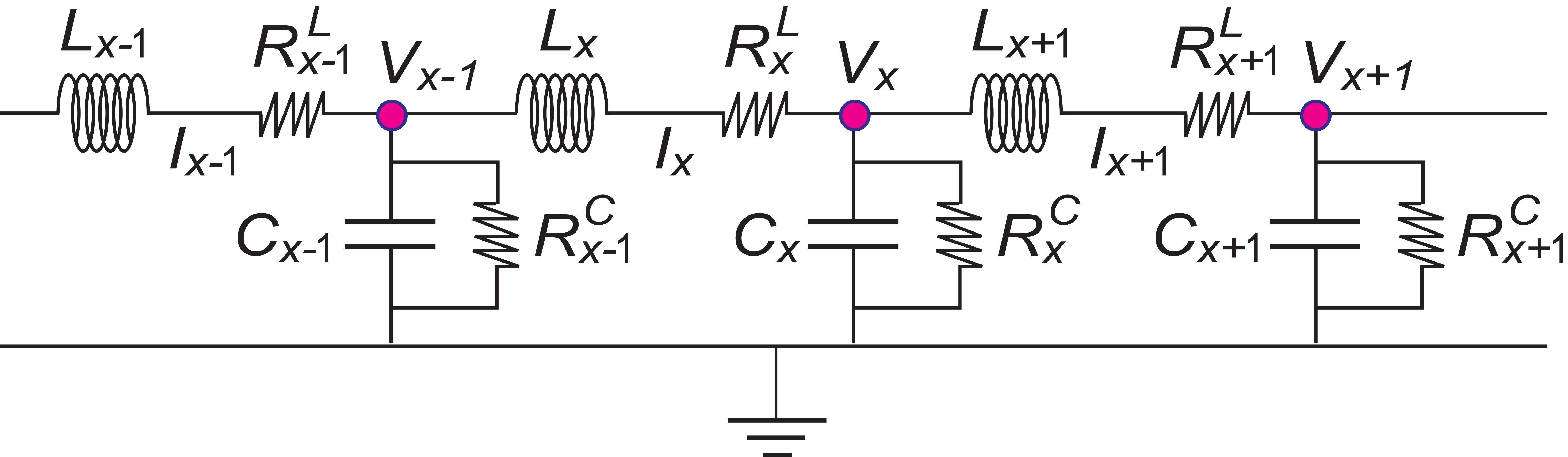
Quantum walk based on $LC$ electric circuits: Our system is a chain of electric circuit shown in Fig.1. It describes the telegrapher equation provided the system is homogeneous. An inhomogeneous circuit is constructed by choosing the sample parameters different depending on the position in a chain. An electric circuit is characterized by the Kirchhoff laws (Fig.1),

$$L_{x}\frac{d}{dt}I_{x}= V_{x-1}-V_{x}-R_{x}^{L}I_{x}.$$ (1)

$$C_{x}\frac{d}{dt}V_{x}= I_{x}-I_{x+1}-V_{x}/R_{x}^{C},$$ (2)

The first equation is the Kirchhoff voltage law with respect to the voltage difference between two nodes $V_{x}$ and $V_{x-1}$, which is equal to the voltage drop by the resistor $R_{x}$ and the inductive electromotive force by the inductor $L_{x}$. The second equation is the Kirchhoff current law with respect to the current conservation at one node $V_{x}$, where the current flows to the ground via the the conductor $C_{x}$ and the resister $R_{x}^{C}$ in paralell. They are combined into a second-order differential equation by deleting $I$ or $V$ in the standard treatmentRosen .

We first analyze the homogeneous case such that $C_{x}=C$, $L_{x}=L$, $R_{x}^{L}=R^{L}$ and $R_{x}^{C}=R^{C}$. We make a scale transformation

$$\mathcal{V}_{k}=V_{k},\qquad\mathcal{I}_{k}=\sqrt{\frac{L}{C}}I_{k},$$ (3)

so that $\mathcal{V}_{k}$ and $\mathcal{I}_{k}$ have the same dimension, where $\sqrt{L/C}I_{k}$ is the voltage drop per unit length. The set of equations (1) and (2) are reformulated in the form of the Schrödinger equation,

$$i\partial_{t}\psi_{k}=\mathcal{H}\left(k\right)\psi_{k},$$ (4)

with the wave function $\psi_{k}=\left(\mathcal{I}_{k},\mathcal{V}_{k}\right)^{t}$, and the Hamiltonian

$$\mathcal{H}\left(k\right)=\left(\begin{array}[]{cc}-i\frac{R^{L}}{L}&-\frac{i}{\sqrt{LC}}\left(1-e^{-ik}\right)\\ \frac{i}{\sqrt{LC}}\left(1-e^{ik}\right)&-i\frac{1}{CR^{C}}\end{array}\right).$$ (5)

This Hamiltonian is non-Hermitian due to the diagonal resister terms $-iR^{C}$ and $-iR^{L}$. The "energy spectrum" is given by

$$E=-i\frac{R^{L}/L+1/CR^{C}}{2}\pm\sqrt{\frac{4}{LC}\sin^{2}k-\left(\frac{R^{L}}{L}-\frac{1}{CR^{C}}\right)^{2}}.$$ (6)

The dynamics is solved as $\psi_{k}\left(t\right)=e^{i\mathcal{H}\left(k\right)t}\psi_{k}\left(0\right)$.

Figure 2: (a) Time evolution of a quantum walk in electric circuits. (b) Time evolution of a quantum walk with nonreciprocity ($\gamma=1.25$) and dissipation ($R=0.4$). The vertical axis is the LDOS constructed from (8), which is the square of voltage. We have set $L_{x}=C_{x}=1$.

For simplicity we set $R^{L}/L=1/CR^{C}=R$. The telegrapher equation is a set of equations (2) and (1), which is converted to

$$i\frac{d}{dt}\psi_{x}=\frac{i}{\sqrt{LC}}\psi_{x-1}-iR\psi_{x}-\frac{i}{\sqrt{LC}}\psi_{x+1},$$ (7)

by transforming (4) into the real space, where we have defined

$$\psi_{x}=\left(\cdots,\mathcal{I}_{x-1},\mathcal{V}_{x-1},\mathcal{I}_{x},\mathcal{V}_{x},\mathcal{I}_{x+1},\mathcal{V}_{x+1},\cdots\right)^{t}.$$ (8)

Let us show that transient phenomena described by (7) together with appropriate initial conditions are mathematically equivalent to the dynamics of quantum walkers.

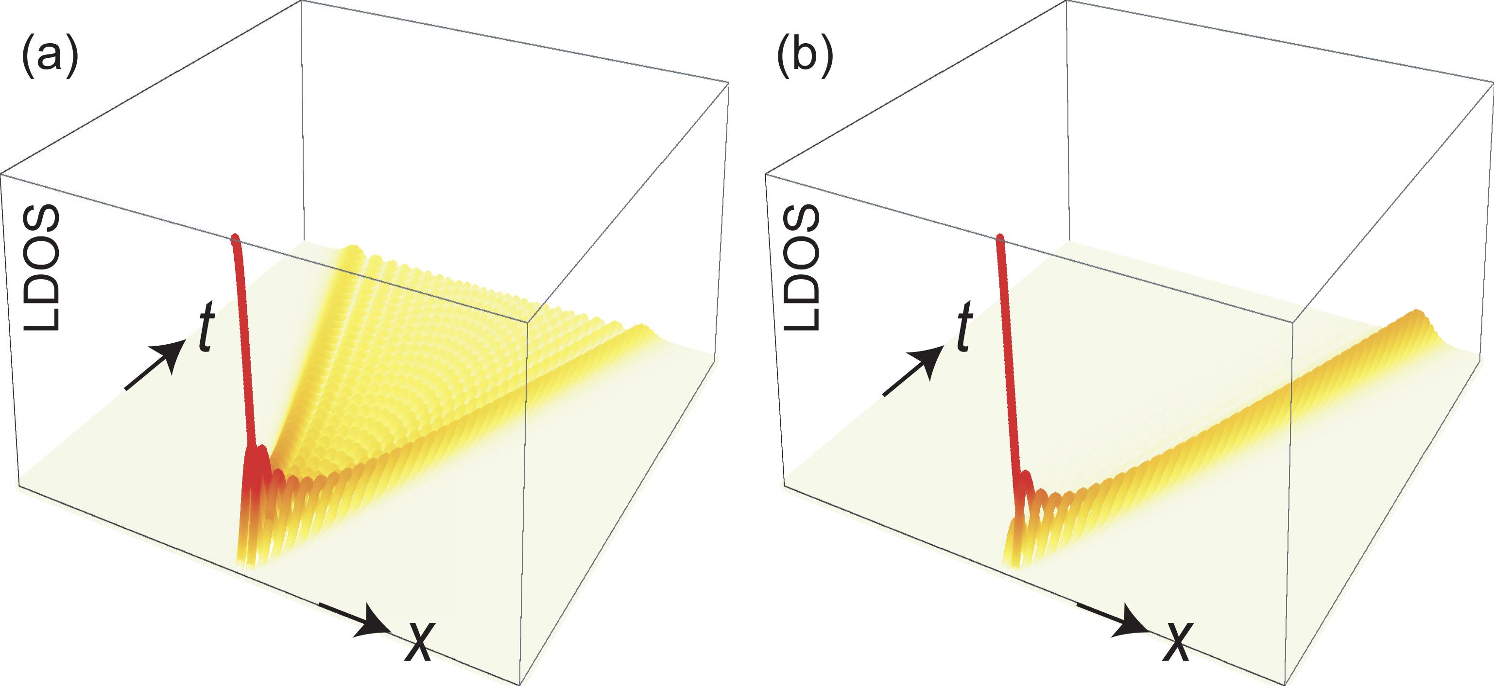
We start with a quantum walker starting from $x=0$ at $t=0$. Namely, we solve (7) by imposing the initial condition $\psi_{x}=\delta_{x0}$ at $t=0$. The analytic solution is obtained as

$$\psi_{x}=e^{-Rt}J_{\left|x\right|}\left(\frac{2}{\sqrt{LC}}t\right),$$ (9)

where $J_{x}$ is the Bessel function. We show the time evolution of the eigenstate in Fig.2(a). The eigenstate is observable by measuring the voltage and the current.

We discuss analytically how the wave packet describing the quantum walker spreads throughout the lattice as shown in Fig.2(a). We define a generating function byKonno

$$G\left(k\right)=\sum_{x=-\infty}^{\infty}\left|\psi_{x}\left(t\right)\right|^{2}e^{kx}.$$ (10)

Using the sum formula of the Bessel function,

$$\sum_{x=-\infty}^{\infty}J_{\left|x\right|}^{2}\left(t\right)e^{kx}=I_{0}\left(t\sqrt{2\left(\cosh k-1\right)}\right),$$ (11)

we find

$$G\left(k\right)=e^{-2Rt}I_{0}\left(2t\sqrt{\frac{2\left(\cosh k-1\right)}{LC}}\right),$$ (12)

where $I_{0}$ is the modified Bessel function. The $n$-th moment is calculated as

$$\left\langle x^{n}\right\rangle=\lim_{k\rightarrow 0}\frac{d^{n}G\left(k\right)}{dk^{n}}.$$ (13)

The total density decreases as

$$\left\langle 1\right\rangle=G\left(0\right)=e^{-2Rt}$$ (14)

in the presence of the dissipation $R$. Indeed, we obtain $\sum_{x=-\infty}^{\infty}\left|\psi_{x}\left(t\right)\right|^{2}=1$ for $R=0$. The mean position is $\left\langle x\right\rangle=0$, while the variance is

$$\left\langle x^{2}\right\rangle=\frac{4t^{2}}{LC}e^{-2Rt}.$$ (15)

Hence, in the absence of the dissipation ($R=0$), the variance diffuses quadratically or the standard deviation increases linearly as a function of time. This is a manifestation of a quantum walkben ; Konno .

Figure 3: Electric-circuit simulation of interference experiment. (a) Time evolution of two quantum walkers starting from two points. (b) Absolute value of the LDOS at a fixed time $t$. The magenta (cyan) curve corresponds to the probability to find the right (left) walker at a certain point, while the black curve corresponds to the probability to find a walker at a certain point. The black curve clearly forms an interference pattern. We have set $L=C=1$, $R=0$ and $t=30$.

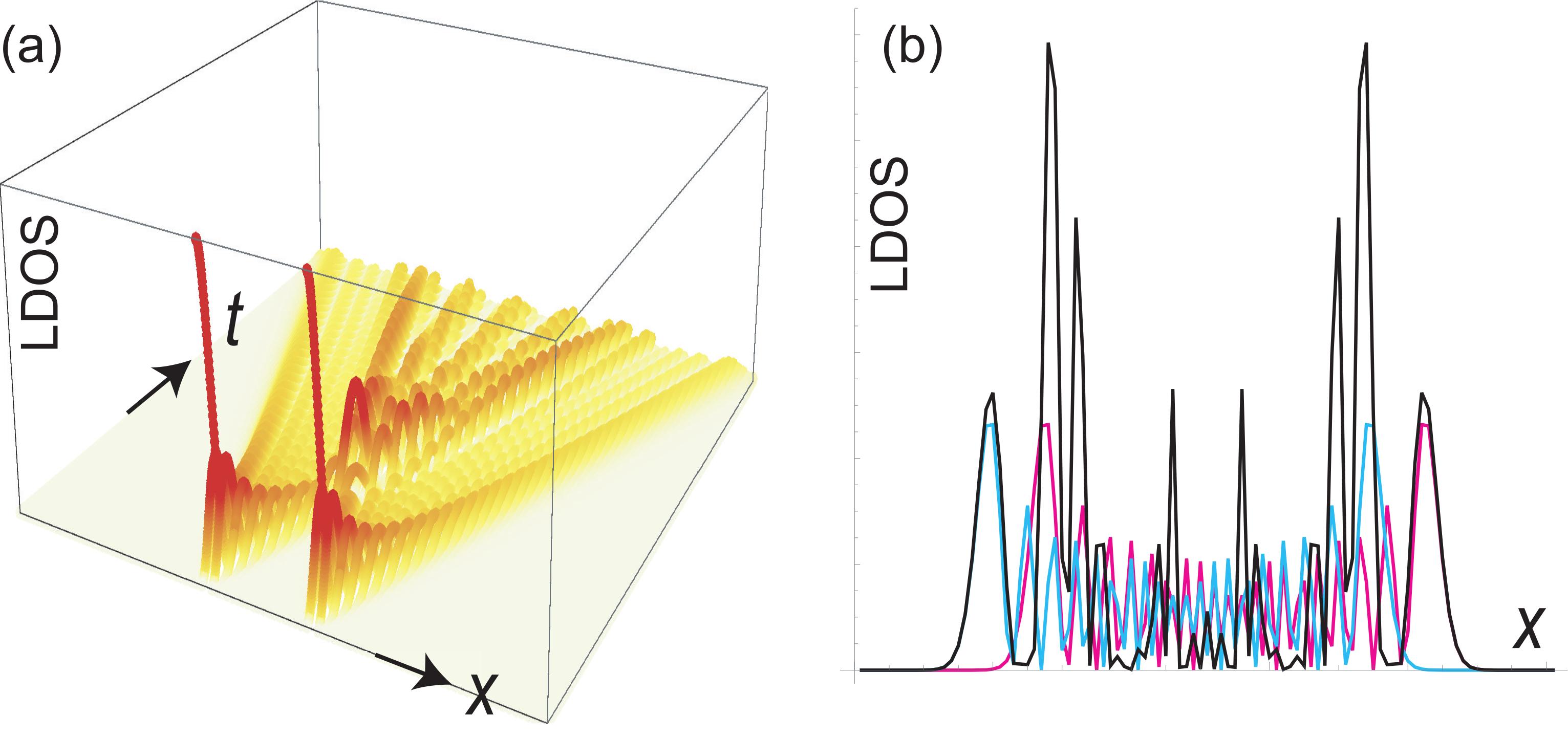
Interference experiment: We analyze the problem of two quantum walkers. Let their starting points be $x\pm x_{0}$ at $t=0$. The eigen function is simply given by a linear superposition of two eigenstates of the type (9),

$$\psi_{x}=\psi_{x}^{+}+\psi_{x}^{-},$$ (16)

where

$$\psi_{x}^{\pm}=e^{-Rt}J_{\left|x\pm x_{0}\right|}\left(\frac{2}{\sqrt{LC}}t\right).$$ (17)

We show the absolute value of $\psi_{x}$ for a fixed time in Fig.3(b). An interference pattern is clearly observed.

Quantum walk in inhomogeneous system: We generalize the results to an inhomogeneous system. By making a spatial dependent scale transformation

$$V_{x}=\alpha_{x}\mathcal{V}_{x},\qquad I_{x}=\beta_{x}\mathcal{I}_{x}$$ (18)

in (1) and (2), we obtain equations

$$i\frac{d}{dt}\mathcal{I}_{x}= \frac{i\alpha_{x-1}}{\beta_{x}L_{x}}\mathcal{V}_{x-1}-\frac{iR_{x}^{L}}{L_{x}}\mathcal{I}_{x}-\frac{i\alpha_{x}}{\beta_{x}L_{x}}\mathcal{V}_{x}.$$ (19)

$$i\frac{d}{dt}\mathcal{V}_{x}= \frac{i\beta_{x}}{\alpha_{x}C_{x}}\mathcal{I}_{x}-\frac{i}{C_{x}R_{x}^{C}}\mathcal{V}_{x}-\frac{i\beta_{x+1}}{\alpha_{x}C_{x}}\mathcal{I}_{x+1},$$ (20)

These equations lead to a non-Hermitian Hamiltonian.

By choosing $\alpha_{x}=\sqrt{C_{1}/C_{x}}$ and $\beta_{x}=\sqrt{C_{1}/L_{x}}$ in (18), the set of equations become

$$i\frac{d}{dt}\mathcal{I}_{x}= i\sqrt{\frac{1}{L_{x}C_{x-1}}}\mathcal{V}_{x-1}-\frac{iR_{x}^{L}}{L_{x}}\mathcal{I}_{x}-i\sqrt{\frac{1}{L_{x}C_{x}}}\mathcal{V}_{x}.$$ (21)

$$i\frac{d}{dt}\mathcal{V}_{x}= i\sqrt{\frac{1}{L_{x}C_{x}}}\mathcal{I}_{x}-\frac{i}{C_{x}R_{x}^{C}}\mathcal{V}_{x}-i\sqrt{\frac{1}{L_{x+1}C_{x}}}\mathcal{I}_{x+1},$$ (22)

When we set $R_{x}^{L}/L_{x}=1/C_{x}R_{x}^{C}=R$ for simplicity, the corresponding tight-binding Hamiltonian has a particularly simple form,

$$H=\sum_{x}t_{x}\left(\left|\psi_{x}\right\rangle\left\langle\psi_{x+1}\right|+\left|\psi_{x+1}\right\rangle\left\langle\psi_{x}\right|\right)-iR\left|\psi_{x}\right\rangle\left\langle\psi_{x}\right|,$$ (23)

with $t_{2x-1}=1/\sqrt{L_{x}C_{x}}$ and $t_{2x}=1/\sqrt{L_{x+1}C_{x}}$. Here, $t_{x}$ represents the hopping parameter between two sites $x$ and $x+1$. The inverse solutions are given by

$$\frac{L_{x}}{L_{1}}=\left(\frac{\prod\limits_{j=1}^{x-1}t_{2j-1}}{\prod\limits_{j=1}^{x-1}t_{2j}}\right)^{2},\qquad\frac{C_{x}}{C_{1}}=\left(\frac{\prod\limits_{j=1}^{x-1}t_{2j+1}}{\prod\limits_{j=1}^{x-1}t_{2j}}\right)^{2}.$$ (24)

Consequently, it is possible to arrange capacitors $C_{x}$ and inductors $L_{x}$ to reproduce various tight-binding models with arbitrary hopping parameters $t_{x}$.

Figure 4: (a) "Energy spectrum" as a function of $\lambda$. There are "zero-energy" edge states indicated by a red line in the topological phase ($\lambda>0$), while there are no edge states in the trivial phase ($\lambda<0$). (b) Time evolution of a quantum walk in the topological phase ($\lambda=0.5$), and (c) that in the trivial phase ($\lambda=-0.5$). A quantum walk does not diffuse for the topological phase, while it diffuses for the trivial phase.

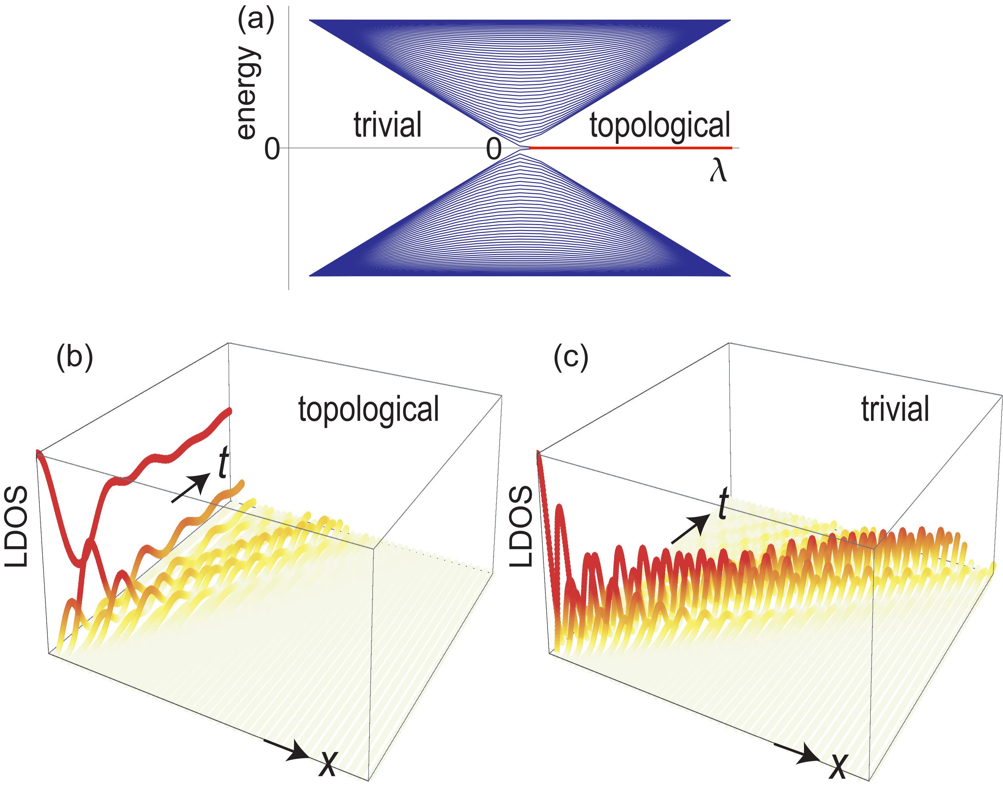
Quantum walks in topological and trivial phases: We proceed to investigate how quantum walks are different in topological and trivial phases. The simplest model possessing these phases is given by the SSH modelSimon . The SSH model is given by the Hamiltonian (23) together with $R=0$ and

$$t_{x}=t+\left(-1\right)^{x}\lambda.$$ (25)

The electric circuit is constructed by choosing inductors and capacitors satisfying (24). The energy spectrum is shown as a function of $\lambda$ in Fig.4(a). There are "zero-energy" edge states for $\lambda>0$, signaling that the system is topological, while the system is trivial for $\lambda<0$ with no edge states. The edges are said topological for $\lambda>0$. These two phases are clearly distinguishable by examining quantum walks. Let a quantum walker start from one of the edges. Namely, we consider the initial state chosen to be perfectly localized at one edge. In the topological phase, a nonzero local density of state (LDOS) remains at the edge as shown in Fig.4(b), while the LDOS rapidly decreases for the trivial phase as shown in Fig.4(c).

These behaviors are understood analytically as follows. By expanding the initial state in terms of the eigenstates as

$$\psi_{x}^{\text{ini}}=\sum_{j}c_{j}\psi_{x}^{\left(j\right)},$$ (26)

the dynamics is given by

$$\psi_{x}\left(t\right)=\sum_{j}c_{j}e^{iE_{j}}\psi_{x}^{\left(j\right)},$$ (27)

where $E_{j}$ is the $j$-th energy, and $\psi_{x}^{\left(j\right)}$ is the eigenstate with the energy $E_{j}$. For the topological phase the coefficient $c_{j}$ has the largest value for the edge state, which has no dynamics. It results in a nonzero LDOS at the edge as in Fig.4(b). On the other hand, there is no dominant $c_{j}$ for the trivial states, which results in the rapid spread of the initial state in Fig.4(c).

Figure 5: (a) Time evolution of the mean value $M(t)$ in electric circuits. (b) Time evolution of the variance $V(t)$. Cyan curves represent a reciprocal quantum walk, while magenta curves represent a nonreciprocal with $\gamma=1.1$ quantum walk. Black dotted lines are asymptotic formula for $t\rightarrow\infty$.

Non-Hermitian nonreciprocal quantum walk: Next, by choosing

$$\alpha_{x}=\gamma^{-2x}\sqrt{\frac{C_{1}}{C_{x}}},\qquad\beta_{x}=\gamma^{-2x+1}\sqrt{\frac{C_{1}}{L_{x}}}$$ (28)

in (18), we construct a non-Hermitian nonreciprocal modelHatano ; UedaPRX ; SkinTop ; EzawaSkin ,

$$H=\sum_{x}t_{x}\left(\gamma\left|\psi_{x}\right\rangle\left\langle\psi_{x+1}\right|+\frac{1}{\gamma}\left|\psi_{x+1}\right\rangle\left\langle\psi_{x}\right|\right)-iR\left|\psi_{x}\right\rangle\left\langle\psi_{x}\right|,$$ (29)

where the parameter $\gamma$ represents the nonreciprocity. The telegrapher equation is given by

$$i\frac{d}{dt}\psi_{x}=\frac{i\gamma}{\sqrt{LC}}\psi_{x-1}-iR\psi_{x}-\frac{i}{\gamma\sqrt{LC}}\psi_{x+1}.$$ (30)

We find an analytic solution

$$\Psi_{x}\left(t\right)=\gamma^{x}e^{-Rt}J_{\left|x\right|}\left(\frac{2}{\sqrt{LC}}t\right).$$ (31)

The generating function is

$$G\left(k\right)=e^{-2Rt}I_{0}\left(2t\sqrt{\frac{\gamma^{2}e^{k}+e^{-k}/\gamma^{2}-2}{LC}}\right).$$ (32)

The total LDOS reads

$$\sum_{x=-\infty}^{\infty}\left|\psi_{x}\left(t\right)\right|^{2}=e^{-2Rt}I_{0}\left(2t\sqrt{\frac{\gamma^{2}+1/\gamma^{2}-2}{LC}}\right).$$ (33)

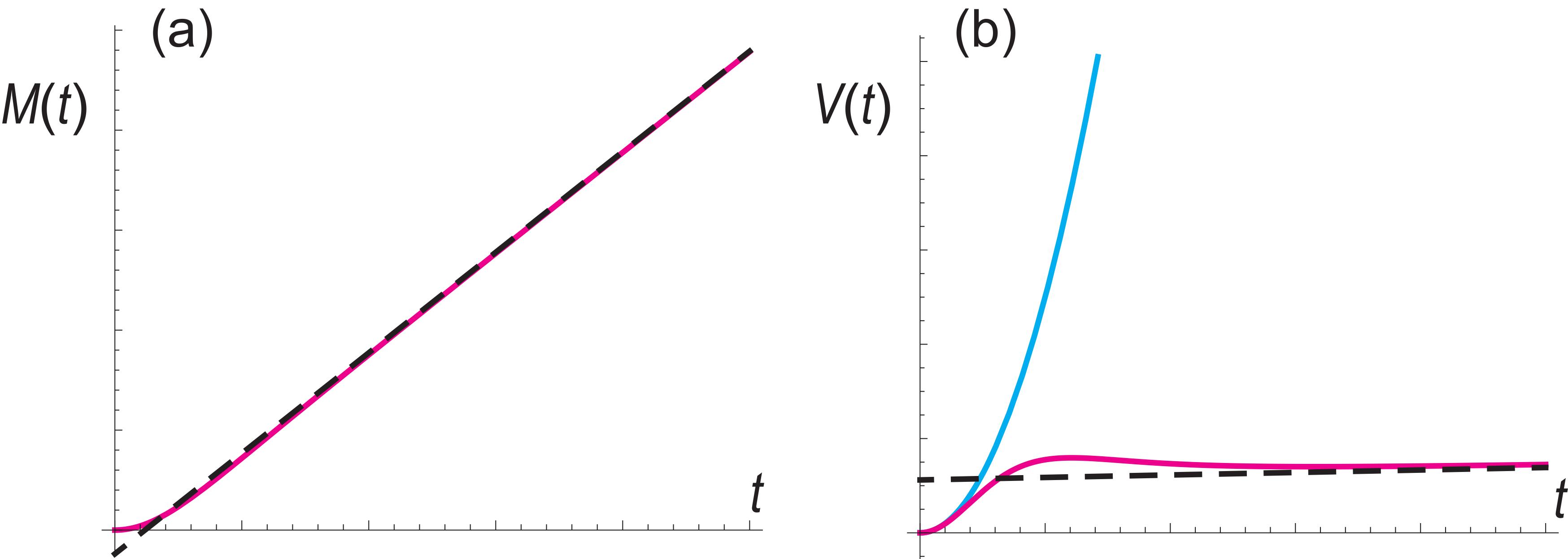
Indeed, it reproduces the result $\left\langle 1\right\rangle\equiv\sum_{x=-\infty}^{\infty}\left|\psi_{n}\left(t\right)\right|^{2}=1$ for $\gamma=1$ and $R=0$. The mean value is defined by $M\left(\Psi\right)=\left\langle x\right\rangle/\left\langle 1\right\rangle$, where we note $\left\langle 1\right\rangle\neq 1$ in general, whose asymptotic behavior is given by

$$\lim_{t\rightarrow\infty}M\left(\Psi\right)$$

$$= \frac{\gamma^{2}-1/\gamma^{2}}{4\left(\gamma^{2}+\frac{1}{\gamma^{2}}-2\right)}\left(\frac{4t}{\sqrt{LC}}\sqrt{\gamma^{2}+\frac{1}{\gamma^{2}}-2}-1\right).$$ (34)

The variance is given by $V\left(\Psi\right)=\left\langle x^{2}\right\rangle/\left\langle 1\right\rangle-M^{2}\left(\Psi\right)$, which reads

$$\lim_{t\rightarrow\infty}V\left(\Psi\right)=\frac{1}{2}\left(\frac{\gamma^{2}}{\left(1-\gamma^{2}\right)^{2}}+\sqrt{\gamma^{2}+\frac{1}{\gamma^{2}}-2}\frac{t}{\sqrt{LC}}\right),$$ (35)

where we have used the asymptotic formula of the modified Bessel function $\lim_{t\rightarrow\infty}I_{0}\left(t\right)=e^{t}/\sqrt{2\pi t}$. We show the time evolution of the mean value and the variance in Fig.5. The asymptotic behaviors well reproduce the analytic results.

Discussions: In this work we have demonstrated that the telegrapher equation and the Schrödinger equation are mathematically equivalent. Consequently, their eigen functions are identical although they describe different physical objects. It is important that the mathematical equivalence justifies us to use the eigen function (8) in the electric-circuit system to simulate the quantum dynamics governed by the Schrödinger equation. As an explicit example, we have derived the oscillatory pattern characteristic to a quantum walk, provided electric circuits are appropriately designed.

We have also studied dissipative and nonreciprocal quantum walks by tuning sample parameters. In a nonreciprocal quantum walk, the variance is proportional to time which is smaller than that in a reciprocal quantum walk, where it is proportional to the square of time. It will be a benefit for future high-speed quantum search. Electric circuits have a merit that they are easily equipped compared with other methods such as photonic, wave-guide and nuclear-magnetic resonant systems. Furthermore, there is a potentiality to construct integrated circuits of quantum walks.

The author is very much grateful to N. Nagaosa and E. Saito for helpful discussions on the subject. This work is supported by the Grants-in-Aid for Scientific Research from MEXT KAKENHI (Grants No. JP17K05490, No. JP15H05854 and No. JP18H03676). This work is also supported by CREST, JST (JPMJCR16F1).

References

- (1) C. H. Lee , S. Imhof, C. Berger, F. Bayer, J. Brehm, L. W. Molenkamp, T. Kiessling and R. Thomale, Communications Physics, 1, 39 (2018).
- (2) S. Imhof, C. Berger, F. Bayer, J. Brehm, L. Molenkamp, T. Kiessling, F. Schindler, C. H. Lee, M. Greiter, T. Neupert, R. Thomale, Nat. Phys. 14, 925 (2018).
- (3) M. S.-Garcia, R. Susstrunk and S. D. Huber, Phys. Rev. B 99, 020304 (2019).
- (4) T. Helbig, T. Hofmann, C. H. Lee, R. Thomale, S. Imhof, L. W. Molenkamp and T. Kiessling, Phys. Rev. B 99, 161114 (2019).
- (5) Y. Lu, N. Jia, L. Su, C. Owens, G. Juzeliunas, D. I. Schuster and J. Simon, Phys. Rev. B 99, 020302 (2019).
- (6) M. Ezawa, Phys. Rev. B 98, 201402(R) (2018).
- (7) T. Hofmann, T. Helbig, C. H. Lee, M. Greiter, R. Thomale, Phys. Rev. Lett. 122, 247702 (2019).
- (8) K. Luo, R. Yu and H. Weng, Research (2018), ID 6793752.
- (9) M. Ezawa, Phys. Rev. B 99, 201411(R) (2019).
- (10) M. Ezawa, Phys. Rev. B 99, 121411(R) (2019).
- (11) M. Ezawa, Phys. Rev. B 100, 081401(R) (2019)
- (12) M. Ezawa, Phys. Rev. B 100, 045407 (2019).
- (13) T. Helbig, T. Hofmann, S. Imhof, M. Abdelghany, T. Kiessling, L. W. Molenkamp, C. H. Lee, A. Szameit, M. Greiter, R. Thomale, arXiv:1907.11562
- (14) Q.-B. Zeng, Y.-B. Yang and Y. Xu, arXiv:1901.08060
- (15) H. Jiang, L.-J. Lang, C Yang, S.-L. Zhu and S. Chen, Phys. Rev. B 100, 054301 (2019)
- (16) C. H. Lee, T. Hofmann, T. Helbig, Y. Liu, X. Zhang, M. Greiter and R. Thomale, cond-mat/arXiv:1904.10183
- (17) Y. Aharonov, L. Davidovich and N. Zagury, Phys. Rev. A, 48, 1687 (1993).
- (18) E. Farhi and S. Gutmann, Phys. Rev. A 58, 915 (1998)
- (19) A. Ambainis, Int. J. Quantum Information, 1, 507 (2003)
- (20) S. E. Venegas-Andraca, Quantum Information Processing, 11, 1015 (2012)
- (21) J. Kempe, Contemporary Physics 44, 307 (2003)
- (22) M. S. Rudner and L. S. Levitov, Phys. Rev. Lett. 102, 065703 (2009).
- (23) D. ben-Avraham, E. M. Bollt and C. Tamon, Quantum Information Processing, 3, 1 (2004)
- (24) N. Konno, Phys. Rev. E, 72 026113 (2005)
- (25) M. Szegedy, in Proceedings of the 45th IEEE Symposium on Foundations of Computer Science (IEEE, New York, 2004), pp. 32-41.
- (26) A. M. Childs and J. Goldstone, Phys. Rev. A 70, 022314 (2004)
- (27) A. M. Childs, Phys. Rev. Lett. 102, 180501 (2009).
- (28) A. M. Childs, D. Gosset, Z. Webb, Science 339, 791 (2013)
- (29) Z. H. Bian, J. Li, H. Qin, X. Zhan, R. Zhang, B. C. Sanders, and P. Xue, Phys. Rev. Lett. 114, 203602 (2015)
- (30) A. Peruzzo, M. Lobino, J. C. F. Matthews, N. Matsuda, A. Politi, K. Poulios, X.-Q. Zhou, Y. Lahini, N. Ismail, K. Worhoff, Y. Bromberg, Y. Silberberg, M. G. Thompson, J. L. O’Brien, Science, 329(5998):1500, (2010)
- (31) A. A. Guzik and P. Walther, Nature Physics 8, 285 (2012)
- (32) T. Kitagawa, M. A. Broome, A. Fedrizzi, M. S. Rudner, E. Berg, I. Kassal, A. Aspuru-Guzik, E. Demler and A. G. White, Nature Communications 3, 882 (2012)
- (33) L. Xiao, X. Zhan, Z. H. Bian, K. K. Wang, X. Zhang, X. P. Wang, J. Li, K. Mochizuki, D. Kim, N. Kawakami, W. Yi, H. Obuse, B. C. Sanders, and P. Xue, Nat. Physics 13, 1117 (2017).
- (34) H. B. Perets, Y. Lahini, F. Pozzi, M. Sorel, R. Morandotti and Y. Silberberg, Phys. Rev. Lett. 100, 170506 (2008)
- (35) J. Du, H. Li, X. Xu, M. Shi, J. Wu, X. Zhou and R. Han, Phys. Rev. A 67, 042316 (2003)
- (36) M. S. Rudner and L. S. Levitov, Phys. Rev. B 82, 155418 (2010)
- (37) E. I. Rosenthal, N. K. Ehrlich, M. S. Rudner, A. P. Higginbotham, and K. W. Lehnert, Phys. Rev. B 97, 220301(R) (2018)
- (38) N. Hatano and D. R. Nelson, Phys. Rev. Lett. 77, 570 (1996): Phys. Rev. B 56, 8651 (1997): Phys. Rev. B 58, 8384 (1998).
- (39) Z. Gong, Y. Ashida, K. Kawabata, K. Takasan, S. Higashikawa and M. Ueda, Phys. Rev. X 8, 031079 (2018).
- (40) C. H. Lee, L. Li and J. Gong, Phys. Rev. Lett. 123, 016805 (2019).
- (41) D. S. Simon, S. Osawa, A. V. Sergienko, arXiv:1808.10066