On the identification of source term in the heat equation from sparse data

Abstract

We consider the recovery of a source term $f(x,t)=p(x)q(t)$ for the nonhomogeneous heat equation in $\Omega\times(0,\infty)$ where $\Omega$ is a bounded domain in $\mathbb{R}^{2}$ with smooth boundary $\partial\Omega$ from overposed lateral data on a sparse subset of $\partial\Omega\times(0,\infty)$. Specifically, we shall require a small finite number $N$ of measurement points on $\partial\Omega$ and prove a uniqueness result; namely the recovery of the pair $(p,q)$ within a given class, by a judicious choice of $N=2$ points. Naturally, with this paucity of overposed data, the problem is severely ill-posed. Nevertheless we shall show that provided the data noise level is low, effective numerical reconstructions may be obtained.

Keywords: inverse problem, heat (diffusion) equation, sparse measurements, multiple unknowns, nonlinearity, uniqueness, regularization, numerical reconstruction.

AMS Subject Classifications: 35R30, 65M32.

1 Introduction

The inverse problem of recovering an unknown source term $f$ in the parabolic equation $u_{t}-\triangle u=f$ from overspecified data on the solution $u$ has a long history, see for example, [1, 10, 7]. A brief summary of this can be encapsulated by the observation that to obtain a term $f=f(x,t)$ will require either knowledge of $u$ over $\mathbb{R}^{n}\times\mathbb{R}$, which is impractical in almost every physical situation, or over a sufficiently dense subset whereby an approximation could be determined. Thus most work has concentrated on one of the special cases $f=q(t)$ or $f=p(x)$ or as a product $f=p(x)q(t)$ where either $q$ or $p$ is known. An exception here is [2] where the problem was considered in $\mathbb{R}\times(0,\infty)$ and $p$ was of compact support.

It has also been observed that the recovery of a spatially unknown $f$ from spatial measurements of $u$ is usually only mildly-ill-conditioned but the recovery from temporal measurements of $u$ is severely ill-posed. The situation for $f=q(t)$ is reversed. In fact, this problem spawned the now well-known notion that to recover an unknown term or coefficient in a partial differential equation one should ideally prescribe data in a “parallel” direction to that of the unknown; giving overposed data in the “orthogonal” direction is likely to be severely ill-posed.

In this paper we shall assume the form $f=p(x)q(t)$ where both $p$ and $q$ are unknown. We shall prescribe extremely sparse time-trace data and show unique recovery within the specified spaces in which $p$ and $q$ are defined although this paucity of data will require quite severe restrictions on the allowable class for the unknown term $q(t)$. The exposition will be much simpler if we take the spatial domain $\Omega$ to be the unit disc in $\mathbb{R}^{2}$. This is not an essential requirement and we could take $\Omega\subset\mathbb{R}^{2}$ to have a smooth $C^{2}$ boundary. We will comment on this fact later.

Let $u(x,t)\in\Omega\times[0,\infty)$ solve

$$\begin{cases}\begin{aligned} \frac{\partial u}{\partial t}(x,t)-\triangle u(x,t)&=p(x)q(t),&&(x,t)\in\Omega\times(0,\infty),\\ u(x,t)&=0,&&(x,t)\in\partial\Omega\times(0,\infty),\\ u(x,0)&=0,&&x\in\Omega.\end{aligned}\end{cases}$$ (1)

As noted, $\Omega$ is the unit disc in $\mathbb{R}^{2}$ and $p$, $q$ are the unknown source sub-functions. Our additional data is of the form of flux measurements at a small number $L$ of points situated on $\partial\Omega$

$$g_{\ell}(t):=\frac{\partial u}{\partial{\overrightarrow{\bf n}}}(z_{\ell},t),\ t\in(0,\infty),\ z_{\ell}\in\partial\Omega,\ \ell=1,2,\ldots\,,L.$$ (2)

A related problem was considered in [6] where it was assumed that $q=1$ and $p=\chi(D)$ for some star-like domain $D\subset\Omega$. Uniqueness in the form of local injectivity of the derivative of the map $D\to g_{\ell}$ was shown: that is recovery of the shape and location of a source of known uniform strength. In this case only two flux measurements were required, that is $L=2$.

Our goal in this paper is to generalize this result to include a nontrivial time-dependent term $q(t)$. Such a modification represents a more realistic physical situation whereby the strength of the source may change with time. We will show an analogous result to that in [6] again requiring only that $L=2$ but it should not be surprising that full generality cannot hold for $q(t)$. We will show that uniqueness holds if $q(t)$ is a sequence of step functions, that is $q(t)=\sum_{k=1}^{K}q_{k}H(t-c_{k})$ where $H(t)$ is the Heaviside function and $\{q_{k},c_{k}\}_{1}^{K}$ will be determined in addition to $p(x)$. Note that the case of $K=\infty$ is allowed. However, the previous result in [6] has very little lee-way for generalization and indeed we have unable to allow simply $p(x)\in L^{\infty}(\Omega)$ which would open the path to allow $p=\chi(D)$ as before. Instead we will have to assume slightly more regularity in $p$ and this will preclude allowing it to represent the characteristic function of a subset $D\subset\Omega$. On the other hand we will be able to approximate this to within any desired accuracy so from a physical standpoint there is no essential loss of generality. We shall show this case with some numerical runs in the final section.

There are many physical applications of this work and we mention only the following. Suppose there is an extended source whose spatial location is only known approximately. This could be a source of pollutant for example. It is also a likely possibility that the output from this source depends on time but that over a small enough period can be considered to be approximately constant. Measurements can only be made at a distance from the source and the number of measurement points is very small, perhaps due to logistics, but also due to a small number of detecting sensors. One could consider this problem to be in all of $\mathbb{R}^{2}$ or assume that it is more localized with given boundary constraints. The latter situation is more complex and is the one taken in this paper.

Thus the main result of this paper is as follows, we shall describe some of the technical definitions involved in the next section.

Theorem 1.

Set the boundary observation points $\{z_{\ell}\}$ as $z_{\ell}=(\cos{\theta_{\ell}},\sin{\theta_{\ell}})$. Then under Assumption (2.1), two boundary flux observations can uniquely determine $(p,q)$ up to multiplication, provided

$$\theta_{1}-\theta_{2}\notin\pi\mathbb{Q},$$ (3)

where $\mathbb{Q}$ is the set of rational numbers.

More precisely, let $(p(x),q(t)),\ (\tilde{p}(x),\tilde{q}(t))$ satisfy Assumption (2.1) and denote the corresponding solutions as $u,\tilde{u}$, respectively. If

$$\frac{\partial u}{\partial{\overrightarrow{\bf n}}}(z_{\ell},t)=\frac{\partial\tilde{u}}{\partial{\overrightarrow{\bf n}}}(z_{\ell},t),\quad t\in(0,\infty),\ \ell=1,2,$$

and the condition (3) is fulfilled, then there exists a constant $C_{0}\neq 0$ such that $p=C_{0}\tilde{p}$ in $L^{2}(\Omega)$ and $q=C_{0}^{-1}\tilde{q}$ on $[0,\infty)$.

This article is outlined as follows. In section 2, we provide several preliminary results and prove some lemmas which play crucial roles in the proof of the main theorem. In section 3, we show the well-definedness and the analytic continuation of the Laplace transform on the flux data, see Lemma (3.3), and three auxiliary lemmas for the uniqueness proof. These allow the completion of the proof of Theorem (1) in section 3.4. Based on the theoretical uniqueness property, we construct an iterative scheme to reconstruct the unknowns $p$, $q$ and several numerical results are reproduced in section 4.

2 Preliminary lemmas and background

2.1 Eigensystem $\{\lambda_{n},\varphi_{n}:n\in\mathbb{N}^{+}\}$

Let $\{\lambda_{n},\varphi_{n}(x):n\in\mathbb{N}^{+}\}$ be eigenpairs of $-\triangle$ on $\Omega$ with Dirichlet boundary conditions. The corresponding eigenfunctions $\{\varphi_{n}\}$ will be used in polar coordinates

$$\varphi_{n}(r,\theta)=\omega_{n}J_{m(n)}(\sqrt{\lambda_{n}}r)\cos{(m(n)\theta+\phi_{n})}.$$ (4)

Remark 2.1.

In the representation of $\varphi_{n}$, $\omega_{n}$ is the normalized coefficient to make sure $\|\varphi_{n}\|_{L^{2}(\Omega)}=1$, $J_{m}$ is the $m$-th order Bessel function and the phase $\phi_{n}$ is $0$ or $-\pi/2$. The eigenvalues $\{\lambda_{n}\}$ are set as the square of the zeros of Bessel functions $\{J_{m}\}$ with integer $m$. By Bourget’s hypothesis, which was proven in [12], there exists no common positive zeros between two Bessel functions with integer orders. After indexing all the eigenvalues by non-decreasing order, with a fixed $n$, we can get the corresponding value of $m$ so that we view $m$ as a function of $n$ and this dependence is reflected in the notation $m(n)$. Since there are two choices $0$ or $-\pi/2$ for $\phi_{n}$, for each eigenvalue $\lambda_{n}$ with nonzero $m(n)$, the multiplicity is two. Thus it has two corresponding eigenfunctions. When $m(n)=0$, the multiplicity is only one since the angular part $\cos{(m(n)\theta-\pi/2)}=\sin{0}$ vanishes on $[0,2\pi)$. This fact is also guaranteed in the more general case of a non-circular domain $\Omega$ by the Krein-Rutman theorem. For more details on the structure of the eigenfunctions, see [4].

Since $-\Delta$ is self-adjoint and positive definite on $\Omega$ with homogeneous Dirichlet boundary condition, $\{\lambda_{n}\}$ will be strictly positive and $\{\varphi_{n}\}$ constitutes an orthonormal basis of $L^{2}(\Omega)$. We index the eigenvalues with non-decreasing order, then we have

$$0<\lambda_{1}\leq\cdots\leq\lambda_{n}\leq\cdots\ \text{(multiplicity counted)},\quad\lim_{n\to\infty}\lambda_{n}=\infty.$$

Remark 2.2.

Here we list some properties of $\{\lambda_{n}\}$ and $J_{m}(x)$ which will be used later.

• By Weyl’s law, $\Omega\subset\mathbb{R}^{2}$ implies $\lambda_{n}=O(n)$.

• $[x^{m+1}J_{m+1}(x)]^{\prime}=x^{m+1}J_{m}(x)$.

• $2mJ_{m}(x)/x=J_{m-1}(x)+J_{m+1}(x)$.

• $2[J_{m}(x)]^{\prime}=J_{m-1}(x)-J_{m+1}(x)$.

The following lemma concerns the estimate for the normalized coefficient $\omega_{n}$.

Lemma 2.1.

For $n\in\mathbb{N}^{+},$ $\{\omega_{n}\}$ are given by

$$\omega_{n}=\begin{cases}2^{1/2}\pi^{-1/2}[J_{m+1}(\lambda_{n}^{1/2})]^{-1},&m(n)\neq 0,\\ \pi^{-1/2}[J_{1}(\lambda_{n}^{1/2})]^{-1},&m(n)=0.\end{cases}$$

Proof.

Since $\|\varphi_{n}\|_{L^{2}(\Omega)}=1,$ then

$$\omega_{n}^{2}\int_{0}^{2\pi}\cos^{2}{(m\theta+\phi_{n})}\,d\theta\ \int_{0}^{1}J_{m}^{2}(\sqrt{\lambda_{n}}r)r\,dr=1.$$

If $m(n)\neq 0$, we have $\int_{0}^{2\pi}\cos^{2}{(m\theta+\phi_{n})}\,d\theta=\frac{1}{2}\int_{0}^{2\pi}{1+\cos{2(m\theta+\phi_{n})}}\,d\theta=\pi$ and

$$\int_{0}^{1}J_{m}^{2}(\sqrt{\lambda_{n}}r)r\,dr =\lambda_{n}^{-1}\int_{0}^{\lambda_{n}^{1/2}}J_{m}^{2}(s)s\,ds$$

$$=\lambda_{n}^{-1}\Big{[}r^{2}J_{m+1}^{2}(r)/2+r^{2}J_{m}^{2}(r)/2-mrJ_{m}(r)J_{m+1}(r)\Big{]}\Big{|}_{0}^{\lambda_{n}^{1/2}}$$

$$=J_{m+1}^{2}(\lambda_{n}^{1/2})/2,$$

where the second result comes from the fact that $\lambda_{n}^{1/2}$ is the zero of $J_{m}(r)$ and the recurrence relations in Remark (2.2). Hence, we have

$$\omega_{n}J_{m+1}(\lambda_{n}^{1/2})=2^{1/2}\pi^{-1/2}.$$

Analogously, for the case of $m(n)=0$, it holds that $\omega_{n}J_{1}(\lambda_{n}^{1/2})=\pi^{-1/2}$ and the proof is complete. ∎

2.2 Assumptions and solution regularities

We give the definitions of the space $\mathcal{D}((-\Delta)^{\gamma})$ and the Heaviside function $H(t)$ that will be used throughout the paper. For $\gamma>0$, define $\mathcal{D}((-\Delta)^{\gamma})\subset L^{2}(\Omega)$ as

$$\mathcal{D}((-\Delta)^{\gamma}):=\{\psi\in L^{2}(\Omega):\sum_{n=1}^{\infty}\lambda_{n}^{2\gamma}\ |\langle\psi(\cdot),\varphi_{n}(\cdot)\rangle_{L^{2}(\Omega)}|^{2}\}<\infty,$$ (5)

here $\langle\cdot,\cdot\rangle_{L^{2}(\Omega)}$ means the inner product in $L^{2}(\Omega)$. Due to $\Omega$ is the unit disc, $\mathcal{D}((-\Delta)^{\gamma})\subset H^{2\gamma}(\Omega)$. Given $0<\gamma_{1}<\gamma_{2}$, since $0<\lambda_{1}\leq\cdots\leq\lambda_{n}\leq\cdots,$ it is not hard to show $\mathcal{D}((-\Delta)^{\gamma_{2}})\subset\mathcal{D}((-\Delta)^{\gamma_{1}}).$

Also, the Heaviside function $H(t)$ is defined in the usual way

$$H(t)=\begin{cases}0,&t<0,\\ 1,&t\geq 0,\end{cases}$$

and it is clear that $\chi_{{}_{[a,b)}}=H(t-a)-H(t-b),\ a<b.$

With these definitions, we require the following assumptions to be valid throughout the paper.

Assumption 2.1.

$p(x)$ and $q(t)$ satisfy the following conditions:

• There exists $\gamma>0$ such that $p(x)\in\mathcal{D}((-\Delta)^{\gamma})$ and $\|p\|_{L^{2}(\Omega)}\neq 0$.

• $q(t)\in L^{1}(0,\infty)$ is a piecewise constant function, or written as a linear combination of Heaviside functions,

  $$q(t)=\sum_{k=1}^{K-1}\beta_{k}\chi_{{}_{[c_{k},c_{k+1})}}=\sum_{k=1}^{K}q_{k}H(t-c_{k}),$$

  where

  $$K\in\mathbb{N}^{+}\cup\{\infty\},\quad 0\leq c_{1}<c_{2}<\cdots,\quad q_{k}\neq 0.$$

  Moreover, there exists $\eta>0$ such that

  $$\inf\{|c_{k}-c_{k+1}|:k=1,\cdots,K-1\}\geq\eta.$$ (6)

Remark 2.3.

The inclusion $q(t)\in L^{1}(0,\infty)$ and the infimum $\eta$ give that

$$\eta\sum_{k=1}^{K-1}|\beta_{k}|\leq\sum_{k=1}^{K-1}|\beta_{k}|\ |c_{k}-c_{k+1}|=\|q\|_{L^{1}(0,\infty)}<\infty,$$

which leads to $\sum_{k=1}^{K-1}|\beta_{k}|<\infty$. Also, we have

$$\|q\|^{2}_{L^{2}(0,\infty)}= \sum_{k=1}^{K-1}|\beta_{k}|^{2}\ |c_{k}-c_{k+1}|=\sum_{k=1}^{K-1}(|\beta_{k}|\ |c_{k}-c_{k+1}|)\ (|\beta_{k}|)$$

$$\leq \Big{[}\sum_{k=1}^{K-1}|\beta_{k}|\ |c_{k}-c_{k+1}|\Big{]}\ \ \Big{[}\sum_{k=1}^{K-1}|\beta_{k}|\Big{]}<\infty,$$

which gives $q\in L^{2}(0,\infty)$.

From the equality $\sum_{k=1}^{K-1}\beta_{k}\chi_{{}_{[c_{k},c_{k+1})}}=\sum_{k=1}^{K}q_{k}H(t-c_{k})$, we derive that for $K<\infty$,

$$q_{1}=\beta_{1},\ q_{K}=-\beta_{K-1},\ q_{k}=\beta_{k}-\beta_{k-1}\ \ \text{for}\ \ 2\leq k\leq K-1,$$

and for $K=\infty$,

$$q_{1}=\beta_{1},\ q_{k}=\beta_{k}-\beta_{k-1}\ \ \text{for}\ \ k\geq 2.$$

Hence,

$$|q_{k}|\leq\sum_{k=1}^{K-1}|\beta_{k}|<\infty,\quad\sum_{k=1}^{K}|q_{k}|\leq 2\sum_{k=1}^{K-1}|\beta_{k}|<\infty.$$

In addition, (6) yields that

$$|c_{k_{1}}-c_{k_{2}}|\geq|k_{1}-k_{2}|\eta,\quad k_{1},k_{2}=1,\cdots,K.$$

In this subsection we also give a regularity result for $\frac{\partial u}{\partial{\overrightarrow{\bf n}}}(\cdot,t)$.

Lemma 2.2.

For a.e. $t\in[0,\infty)$, $\frac{\partial u}{\partial{\overrightarrow{\bf n}}}(\cdot,t)\in C^{0,2\gamma}(\partial\Omega).$

Proof.

From Assumption (2.1), we have $p(x)\in\mathcal{D}((-\Delta)^{\gamma})$ and $\gamma>0$. Since $\mathcal{D}((-\Delta)^{\gamma_{2}})\subset\mathcal{D}((-\Delta)^{\gamma_{1}})$ if $0<\gamma_{1}<\gamma_{2}$, we can set $\gamma\in(0,1/4)$. In addition, recalling $q(t)\in L^{2}(0,\infty)$, then we have $p(x)q(t)\in L^{2}(0,\infty;\mathcal{D}((-\Delta)^{\gamma}))$. From the spectral representation of $u$, the following regularity holds

$$u\in L^{2}(0,\infty;\mathcal{D}((-\Delta)^{\gamma+1}))\subset L^{2}(0,\infty;H^{2\gamma+2}(\Omega)).$$

Then using the continuity of the trace map $\psi\in H^{2\gamma+2}(\Omega)\mapsto\frac{\partial\psi}{\partial{\overrightarrow{\bf n}}}\in H^{2\gamma+1/2}(\partial\Omega),$ which is [8, Theorem 9.4], gives that for a.e. $t\in[0,\infty)$, $\frac{\partial u}{\partial{\overrightarrow{\bf n}}}(\cdot,t)\in H^{2\gamma+1/2}(\partial\Omega)$. Note that $\partial\Omega$ is one-dimensional and $2\gamma+1/2\in(1/2,1)$, which mean the conditions of [3, Theorem 8.2] are satisfied. Then we have $\frac{\partial u}{\partial{\overrightarrow{\bf n}}}(\cdot,t)\in C^{0,2\gamma}(\partial\Omega)$ and this completes the proof. ∎

3 Uniqueness

This section is devoted to the proof of the main theoretical result, Theorem (1).

3.1 Harmonic functions and measurements representations

First, we need to show how to connect the boundary flux measurements $\frac{\partial u}{\partial{\overrightarrow{\bf n}}}|_{\partial\Omega}$ and the unknowns $p(x),\ q(t)$. Here we introduce the harmonic functions $\{\xi_{j}:j\in\mathbb{N}^{+}\}$ which will be used to represent measurements. The set of harmonic functions with domain $(r,\theta)\in[0,1]\times[0,2\pi)$ is defined as

$$\xi_{j}(r,\theta) =\begin{cases}\pi^{-1/2}r^{l}\cos{l\theta},&j=2l+1,\ l>0,\\ 2^{-1/2}\pi^{-1/2},&j=1,\\ \pi^{-1/2}r^{l}\sin{l\theta},&j=2l,\ l>0,\end{cases}$$

$$=\begin{cases}\pi^{-1/2}r^{\lfloor j/2\rfloor}\cos{\big{(}\lfloor j/2\rfloor\theta+\sigma_{j}\big{)}},&j>1,\\ 2^{-1/2}\pi^{-1/2},&j=1.\end{cases}$$

Here $\lfloor j/2\rfloor$ means the largest integer which is not larger than $j/2$ and

$$\sigma_{j}=\begin{cases}0,&j\ \text{is odd},\\ -\pi/2,&j\ \text{is even}.\end{cases}$$

Fixing $r=1,$ the set

$$\{\xi_{j}(1,\theta):j\in\mathbb{N}^{+},\ \theta\in[0,2\pi)\}=\{2^{-1/2}\pi^{-1/2},\ \pi^{-1/2}\sin{(l\theta)},\ \pi^{-1/2}\cos{(l\theta)}:l\in\mathbb{N}^{+}\}$$

will form an orthonormal basis in $L^{2}(\partial\Omega)$.

Fix $z=(\cos{\theta_{z}},\sin{\theta_{z}})\in\partial\Omega$, let’s calculate $\langle\xi_{j}(z)\xi_{j}(\cdot),\varphi_{n}(\cdot)\rangle_{L^{2}(\Omega)}$. For $n\in\mathbb{N}^{+}$ define

$$a_{n}(z) =\begin{cases}2^{1/2}\pi^{-1/2}\lambda_{n}^{-1/2}\cos{(m(n)\theta_{z}+\phi_{n})},&m(n)\neq 0,\\ \pi^{-1/2}\lambda_{n}^{-1/2},&m(n)=0,\end{cases}$$ (7)

$$p_{n} =\langle p(\cdot),\varphi_{n}(\cdot)\rangle_{L^{2}(\Omega)}.$$

Reference [6] shows that $\langle\xi_{j}(z)\xi_{j}(\cdot),\varphi_{n}(\cdot)\rangle_{L^{2}(\Omega)}$ can be written as a product of three terms:

$$\cos{(\lfloor j/2\rfloor\theta_{z}+\sigma_{j})},\quad\int_{0}^{2\pi}\!\cos(m\theta+\phi_{n})\cos{(\lfloor j/2\rfloor\theta+\sigma_{j})}\,d\theta,\quad\omega_{n}\int_{0}^{1}r^{\lfloor j/2\rfloor+1}J_{m}(\lambda_{n}^{1/2}r)\,dr$$

and a factor of $\pi^{-1}$ or $2^{-1}\pi^{-1}$. The integral in the angular variable $\theta$, and hence the inner product, is zero except when $m=\lfloor j/2\rfloor$ and $\phi_{n}=\sigma_{j}$ in which case it has value $\pi$ or $2\pi$. The integral in the radial variable $r$ can then be written as $\int_{0}^{1}r^{m+1}J_{m}(\lambda_{n}^{1/2}r)\,dr$ and after a change of variable $s=\lambda_{n}^{1/2}r$ and use of a Bessel function recursion formula, becomes

$$\lambda_{n}^{-1-m/2}\int_{0}^{\lambda_{n}^{1/2}}s^{m+1}J_{m}(s)\,ds=\lambda_{n}^{-1/2}J_{m+1}(\lambda_{n}^{1/2}).$$

Thus combining all the terms and using Lemma (2.1) show that

$$\langle\xi_{j}(z)\xi_{j}(\cdot),\varphi_{n}(\cdot)\rangle_{L^{2}(\Omega)}= \begin{cases}(\frac{2}{\pi\lambda_{n}})^{1/2}\cos{(m\theta_{z}+\phi_{n})},&\text{if}\ m(n)=\lfloor j/2\rfloor\neq 0\ \text{and}\ \phi_{n}=\sigma_{j},\\ (\pi\lambda_{n})^{-1/2},&\text{if}\ m(n)=\lfloor j/2\rfloor=0,\\ 0,&\text{otherwise},\end{cases}$$ (8)

$$= \begin{cases}a_{n}(z),&\text{if}\ m(n)=\lfloor j/2\rfloor\ \text{and}\ \phi_{n}=\sigma_{j},\\ 0,&\text{otherwise}.\end{cases}$$

Now we use the Harmonic basis $\{\xi_{j}:j\in\mathbb{N}^{+}\}$ to build a connection between the boundary flux $\partial u(z,t)/\partial{\overrightarrow{\bf n}}$ and source terms $p(x),q(t)$.

Fix a point $z\in\partial\Omega$ and define $\psi_{z}^{M}\in C^{\infty}(\overline{\Omega})$ as

$$\psi_{z}^{M}(x)=\sum_{j=1}^{M}\xi_{j}(z)\xi_{j}(r,\theta),\quad(r,\theta)\in[0,1]\times[0,2\pi).$$ (9)

Then we denote the solutions of the following systems by $\{u_{z}^{M}\}$,

$$\begin{cases}\begin{aligned} \frac{\partial u_{z}^{M}}{\partial t}(x,t)-\triangle u_{z}^{M}(x,t)&=0,&&(x,t)\in\Omega\times(0,\infty),\\ u_{z}^{M}(x,t)&=0,&&(x,t)\in\partial\Omega\times(0,\infty),\\ u_{z}^{M}(x,0)&=-\psi_{z}^{M},&&x\in\Omega,\end{aligned}\end{cases}$$ (10)

and require the lemma below.

Lemma 3.1.

Let $w_{z}^{M}=u_{z}^{M}+\psi_{z}^{M},$ then we have

$$-\int_{0}^{t}\frac{\partial u}{\partial{\overrightarrow{\bf n}}}(z,\tau)\ d\tau=\int_{0}^{t}q(\tau)\ \Big{[}\lim_{M\to\infty}\big{\langle}p(\cdot),w_{z}^{M}(\cdot,t-\tau)\big{\rangle}_{L^{2}(\Omega)}\Big{]}\ d\tau.$$

Proof.

Since $\psi_{z}^{M}$ is the linear combination of harmonic functions on $\Omega,$ then

$$\frac{\partial\psi_{z}^{M}}{\partial t}-\triangle\psi_{z}^{M}=0.$$

This result and (10) show that $w_{z}^{M}$ satisfies the equation

$$\frac{\partial w_{z}^{M}}{\partial t}-\triangle w_{z}^{M}=0,\ \ (x,t)\in\Omega\times(0,\infty)$$

with zero initial condition and the boundary condition $w_{z}^{M}|_{\partial\Omega}=\psi_{z}^{M}|_{\partial\Omega}$. Thus Green’s identities show that for each $v\in H_{0}^{1}(\Omega)$,

$$\int_{\Omega}\frac{\partial w_{z}^{M}}{\partial t}(x,t)\ v(x)+\triangledown w_{z}^{M}(x,t)\cdot\triangledown v(x)\ dx=0,\ \ t\in(0,\infty).$$

By a direct calculation we obtain

$$\int_{0}^{t}\int_{\Omega}p(x)q(\tau)w_{z}^{M}(x,t-\tau)\ dx\ d\tau=\int_{0}^{t}\int_{\Omega}\left[\frac{\partial u}{\partial t}(x,\tau)-\triangle u(x,\tau)\right]\ w_{z}^{M}(x,t-\tau)\ dx\ d\tau.$$

Green’s identities and the vanishing initial conditions of $u$ and $w_{z}^{M}$ give that

$$\int_{0}^{t}\int_{\Omega}\frac{\partial u}{\partial t}(x,\tau)\ w_{z}^{M}(x,t-\tau)\ dx\ d\tau= \int_{0}^{t}\int_{\Omega}\frac{\partial w_{z}^{M}}{\partial t}(x,t-\tau)u(x,\tau)\ dx\ d\tau,$$

$$\int_{0}^{t}\int_{\Omega}-\triangle u(x,\tau)\ w_{z}^{M}(x,t-\tau)\ dx\ d\tau= \int_{0}^{t}\int_{\Omega}\triangledown u(x,\tau)\cdot\triangledown w_{z}^{M}(x,t-\tau)\ dx\ d\tau$$

$$-\int_{0}^{t}\int_{\partial\Omega}\frac{\partial u}{\partial{\overrightarrow{\bf n}}}(x,\tau)\psi_{z}^{M}(x)\ dx\ d\tau.$$

Hence,

$$\int_{0}^{t}\int_{\Omega}p(x)q(\tau)w_{z}^{M}(x,t-\tau)\ dx\ d\tau= \int_{0}^{t}\int_{\Omega}\Big{[}\frac{\partial w_{z}^{M}}{\partial t}(x,t-\tau)\ u(x,\tau)$$

$$\qquad\quad+\triangledown w_{z}^{M}(x,t-\tau)\cdot\triangledown u(x,\tau)\Big{]}\ dx\ d\tau$$

$$-\int_{0}^{t}\int_{\partial\Omega}\frac{\partial u}{\partial{\overrightarrow{\bf n}}}(x,\tau)\psi_{z}^{M}(x)\ dx\ d\tau$$

$$= -\int_{0}^{t}\sum_{j=1}^{M}\xi_{j}(z)\ \big{\langle}\frac{\partial u}{\partial{\overrightarrow{\bf n}}}(\cdot,\tau),\xi_{j}(\cdot)\big{\rangle}_{L^{2}(\partial\Omega)}\ d\tau.$$

The smoothness property $\frac{\partial u}{\partial{\overrightarrow{\bf n}}}(\cdot,t)\in C^{0,2\gamma}(\partial\Omega)$ in Lemma (2.2) ensures that the Fourier series of $\frac{\partial u}{\partial{\overrightarrow{\bf n}}}(\cdot,t)$ converges pointwisely on $\partial\Omega$, namely

$$\lim_{M\to\infty}\sum_{j=1}^{M}\xi_{j}(z)\ \big{\langle}\frac{\partial u}{\partial{\overrightarrow{\bf n}}}(\cdot,\tau),\xi_{j}(\cdot)\big{\rangle}_{L^{2}(\partial\Omega)}=\frac{\partial u}{\partial{\overrightarrow{\bf n}}}(z,\tau),\quad a.e.\ \tau\in(0,t).$$

Since the ‘almost everywhere’ does not effect the result of integral, we have

$$-\int_{0}^{t}\frac{\partial u}{\partial{\overrightarrow{\bf n}}}(z,\tau)\ d\tau =-\int_{0}^{t}\Big{[}\lim_{M\to\infty}\sum_{j=1}^{M}\xi_{j}(z)\ \big{\langle}\frac{\partial u}{\partial{\overrightarrow{\bf n}}}(\cdot,\tau),\xi_{j}(\cdot)\big{\rangle}_{L^{2}(\partial\Omega)}\Big{]}\ d\tau$$

$$=\int_{0}^{t}q(\tau)\ \Big{[}\lim_{M\to\infty}\big{\langle}p(\cdot),w_{z}^{M}(\cdot,t-\tau)\big{\rangle}_{L^{2}(\Omega)}\Big{]}\ d\tau.$$

∎

With the above lemma, the next corollary follows.

Corollary 3.1.

Fix $z=(\cos{\theta_{z}},\sin{\theta_{z}})\in\partial\Omega$, then

$$-\int_{0}^{t}\frac{\partial u}{\partial{\overrightarrow{\bf n}}}(z,\tau)\ d\tau=\int_{0}^{t}q(\tau)\ \Big{[}\sum_{n=1}^{\infty}a_{n}(z)p_{n}[1-e^{-\lambda_{n}(t-\tau)}]\Big{]}\ d\tau.$$

Proof.

For each $M\in\mathbb{N}^{+}$, from (9) we have $\psi_{z}^{M}\in L^{2}(\Omega)$. Then the Fourier expansion of $\psi_{z}^{M}$ can be given as $\psi_{z}^{M}=\sum_{n=1}^{\infty}a_{n}^{M}(z)\varphi_{n}$, and from $w_{z}^{M}=u_{z}^{M}+\psi_{z}^{M}$ we obtain

$$w_{z}^{M}(x,t)=\sum_{n=1}^{\infty}a_{n}^{M}(z)(1-e^{-\lambda_{n}t})\varphi_{n}(x).$$

The above representation and the regularity $\psi_{z}^{M}\in L^{2}(\Omega)$ give that $w_{z}^{M}(\cdot,t)\in L^{2}(\Omega)$ for $t\in[0,\infty)$. Since $p,w_{z}^{M}(x,t)$ both belong to $L^{2}(\Omega)$, we have

$$\big{\langle}p(\cdot),w_{z}^{M}(\cdot,t)\big{\rangle}_{L^{2}(\Omega)}=\sum_{n=1}^{\infty}a_{n}^{M}(z)p_{n}(1-e^{-\lambda_{n}t}).$$

(8) shows that

$$a_{n}^{M}(z)=\begin{cases}a_{n}(z),&m(n)<M/2,\\ 0,&m(n)>M/2,\end{cases}$$

and for the case of $m(n)=M/2$,

$$a_{n}^{M}(z)=\begin{cases}a_{n}(z),&\sigma_{n}=-\pi/2,\\ 0,&\sigma_{n}=0.\end{cases}$$

These results mean that $a_{n}^{M}(z)=a_{n}(z)$ if $M$ is large, and $|a_{n}^{M}(z)|\leq|a_{n}(z)|$ for each $n,M$.

Given $\epsilon>0$, Lemma (3.2), which will be proved in the next subsection, yields that there exists large $l>0$ such that $\sum_{n=l}^{\infty}|a_{n}(z)p_{n}|<\epsilon$. From the above results for $a_{n}^{M}(z)$, we can find a $M_{0}$ such that if $M\geq M_{0}$, $a_{n}^{M}(z)=a_{n}(z)$ for $n=1,\cdots,l-1$. So for $M\geq M_{0}$,

$$\Big{|}\sum_{n=1}^{\infty}a_{n}^{M}(z)p_{n}(1-e^{-\lambda_{n}t})-\sum_{n=1}^{\infty}a_{n}(z)p_{n}(1-e^{-\lambda_{n}t})\Big{|}= \Big{|}\sum_{n=l}^{\infty}[a_{n}^{M}(z)-a_{n}(z)]p_{n}(1-e^{-\lambda_{n}t})\Big{|}$$

$$\leq 2\sum_{n=l}^{\infty}[|a_{n}^{M}(z)|+|a_{n}(z)|]\ |p_{n}|$$

$$\leq 4\sum_{n=l}^{\infty}|a_{n}(z)p_{n}|<4\epsilon.$$

This in turn leads to

$$\lim_{M\to\infty}\big{\langle}p(\cdot),w_{z}^{M}(\cdot,t)\big{\rangle}_{L^{2}(\Omega)}=\lim_{M\to\infty}\sum_{n=1}^{\infty}a_{n}^{M}(z)p_{n}(1-e^{-\lambda_{n}t})=\sum_{n=1}^{\infty}a_{n}(z)p_{n}(1-e^{-\lambda_{n}t}),$$

which together with Lemma (3.1) completes the proof. ∎

3.2 A Laplace transform analysis

The uniqueness proof relies on the Laplace transform on the result in Corollary (3.1). Before to analyze the Laplace transform, we need the following absolute convergence result.

Lemma 3.2.

$\sum_{n=1}^{\infty}a_{n}(z)p_{n}$ is absolute convergent for each $z\in\partial\Omega$.

Proof.

By the Cauchy-Schwartz inequality,

$$\sum_{n=1}^{\infty}|a_{n}(z)p_{n}| =\sum_{n=1}^{\infty}|a_{n}(z)\lambda_{n}^{-\gamma}|\ |\lambda_{n}^{\gamma}p_{n}|$$

$$\leq\Big{[}\sum_{n=1}^{\infty}a^{2}_{n}(z)\lambda_{n}^{-2\gamma}\Big{]}^{1/2}\ \Big{[}\sum_{n=1}^{\infty}\lambda_{n}^{2\gamma}p_{n}^{2}\Big{]}^{1/2}.$$

$p(x)\in\mathcal{D}((-\Delta)^{\gamma})$ means that $\sum_{n=1}^{\infty}\lambda_{n}^{2\gamma}p_{n}^{2}<\infty.$ Also, from $\lambda_{n}=O(n)$, we have

$$a^{2}_{n}(z)\lambda_{n}^{-2\gamma}\leq C|\lambda_{n}^{-1/2}\lambda_{n}^{-\gamma}|^{2}\leq Cn^{-1-2\gamma},$$

which gives $\sum_{n=1}^{\infty}a^{2}_{n}(z)\lambda_{n}^{-2\gamma}<\infty$. Hence we have $\sum_{n=1}^{\infty}|a_{n}(z)p_{n}|<\infty$ and completes the proof. ∎

Then from Corollary (3.1), taking Laplace transform on $-\int_{0}^{t}\frac{\partial u}{\partial{\overrightarrow{\bf n}}}(z,\tau)\,d\tau$ w.r.t $t$ gives that

$$\mathcal{L}\big{(}-\int_{0}^{t}\frac{\partial u}{\partial{\overrightarrow{\bf n}}}(z,\tau)\,d\tau\big{)}(s)=\mathcal{L}\big{(}q(t)\big{)}(s)\ \ \mathcal{L}\big{(}\sum_{n=1}^{\infty}a_{n}(z)p_{n}[1-e^{-\lambda_{n}t}]\big{)}(s).$$

Since $q(t)\in L^{1}(0,\infty)$ is a piecewise constant function, it is bounded and $\mathcal{L}\big{(}q(t)\big{)}(s)$ is convergent and well-defined for $\operatorname{Re}s>0$. Again, it follows directly that

$$s\mathcal{L}\big{(}q(t)\big{)}(s)=\sum_{k=1}^{K}q_{k}e^{-c_{k}s},\ \operatorname{Re}s>0.$$

From Lemma (3.2) and $|1-e^{-\lambda_{n}t}|\leq 1$, the series $\sum_{n=1}^{\infty}a_{n}(z)p_{n}[1-e^{-\lambda_{n}t}]$ is also uniformly bounded on $(0,\infty)$. This means its Laplace transform is well-defined for $\operatorname{Re}s>0$ and the dominated convergence theorem can be applied to calculate the transform as

$$\mathcal{L}\big{(}\sum_{n=1}^{\infty}a_{n}(z)p_{n}[1-e^{-\lambda_{n}t}]\big{)}(s) =\int_{0}^{\infty}\sum_{n=1}^{\infty}a_{n}(z)p_{n}[e^{-st}-e^{-(s+\lambda_{n})t}]\,dt$$ (11)

$$=\sum_{n=1}^{\infty}a_{n}(z)p_{n}\int_{0}^{\infty}e^{-st}-e^{-(s+\lambda_{n})t}\,dt$$

$$=\sum_{n=1}^{\infty}a_{n}(z)p_{n}\lambda_{n}s^{-1}(s+\lambda_{n})^{-1},\quad\operatorname{Re}s>0.$$

Now we have

$$s^{2}\ \mathcal{L}\big{(}-\int_{0}^{t}\frac{\partial u}{\partial{\overrightarrow{\bf n}}}(z,\tau)\,d\tau\big{)}(s)=\Big{[}\sum_{k=1}^{K}q_{k}e^{-c_{k}s}\Big{]}\ \Big{[}\sum_{n=1}^{\infty}a_{n}(z)p_{n}\lambda_{n}(s+\lambda_{n})^{-1}\Big{]},\quad\operatorname{Re}s>0.$$ (12)

We will show the well-definedness and the analyticity for the above complex-valued functions.

Lemma 3.3.

Under Assumption (2.1), the following properties hold.

• For $R\in\mathbb{R}$, define $\mathbb{C}_{R}:=\{s\in\mathbb{C}:\operatorname{Re}s>R\}$. Then $\sum_{n=1}^{\infty}a_{n}(z)p_{n}\lambda_{n}(s+\lambda_{n})^{-1}$ is uniformly convergent for $s\in\mathbb{C}_{R}\setminus\{-\lambda_{n}:n\in\mathbb{N}^{+}\}$.

• $\sum_{n=1}^{\infty}a_{n}(z)p_{n}\lambda_{n}(s+\lambda_{n})^{-1}$ is analytic on $\mathbb{C}\setminus\{-\lambda_{n}:n\in\mathbb{N}^{+}\}$.

• $\sum_{k=1}^{K}q_{k}e^{-c_{k}s}$ is analytic on $\mathbb{C}^{+}:=\{s\in\mathbb{C}:\operatorname{Re}s\geq 0\}$.

Proof.

For $(a)$, since $0<\lambda_{1}\leq\cdots\leq\lambda_{n}\leq\cdots\to\infty$, there exists a large $N_{1}$ such that $\lambda_{n}>2|R|$ for $n\geq N_{1}$. Then for $s\in\mathbb{C}_{R}\setminus\{-\lambda_{n}:n\in\mathbb{N}^{+}\}$ and $n\geq N_{1}$,

$$|s+\lambda_{n}|\geq|\operatorname{Re}s+\lambda_{n}|=\lambda_{n}+\operatorname{Re}s\geq\lambda_{n}-|R|>0,$$

which gives

$$|\lambda_{n}(s+\lambda_{n})^{-1}|=\lambda_{n}|s+\lambda_{n}|^{-1}\leq\lambda_{n}(\lambda_{n}-|R|)^{-1}<2.$$

Given $\epsilon>0,$ Lemma (3.2) yields that there exists $N_{2}$ such that for $l\geq N_{2}$,

$$\sum_{n=l}^{\infty}|a_{n}(z)p_{n}|<\epsilon.$$

So, for $l\geq\max\{N_{1},N_{2}\}$ and $s\in\mathbb{C}_{R}\setminus\{-\lambda_{n}:n\in\mathbb{N}^{+}\}$,

$$\big{|}\sum_{n=l}^{\infty}a_{n}(z)p_{n}\lambda_{n}(s+\lambda_{n})^{-1}\big{|}\leq\sum_{n=l}^{\infty}|a_{n}(z)p_{n}|\ |\lambda_{n}(s+\lambda_{n})^{-1}|\leq 2\sum_{n=l}^{\infty}|a_{n}(z)p_{n}|<2\epsilon,$$

which implies the uniform convergence.

For $(b)$, it is clear that $a_{n}(z)p_{n}\lambda_{n}(s+\lambda_{n})^{-1}$ is holomorphic on $\mathbb{C}_{R}$. Then the uniform convergence gives that $\sum_{n=1}^{\infty}a_{n}(z)p_{n}\lambda_{n}(s+\lambda_{n})^{-1}$ is holomorphic, i.e. analytic on $\mathbb{C}_{R}$ for each $R\in\mathbb{R}$. Given $s\in\mathbb{C}\setminus\{-\lambda_{n}:n\in\mathbb{N}^{+}\}$, we can find a $R$ such that $s\in\mathbb{C}_{R}$, which means $\sum_{n=1}^{\infty}a_{n}(z)p_{n}\lambda_{n}(s+\lambda_{n})^{-1}$ is analytic on $\mathbb{C}\setminus\{-\lambda_{n}:n\in\mathbb{N}^{+}\}$.

For $(c)$, it is obviously valid if $K<\infty$. This is because $q_{k}e^{-c_{k}s}$ is analytic on $\mathbb{C}^{+}$ and the sum is finite. For the case of $K=\infty$, following the proofs for $(a)$ and $(b)$, we have

$$\big{|}\sum_{k=l}^{\infty}q_{k}e^{-c_{k}s}\big{|}\leq\sum_{k=l}^{\infty}|q_{k}|\ |e^{-c_{k}s}|\leq\sum_{k=l}^{\infty}|q_{k}|,\quad s\in\mathbb{C}^{+},\ l\in\mathbb{N}^{+}.$$

This result together with the absolute convergence of $\sum_{k=1}^{\infty}q_{k}$, stated by Remark (2.3), yields the uniform convergence of $\sum_{k=1}^{\infty}q_{k}e^{-c_{k}s}$ on $\mathbb{C}^{+}$. Then with the analyticity of each component function $q_{k}e^{-c_{k}s}$, we can deduce that $\sum_{k=1}^{\infty}q_{k}e^{-c_{k}s}$ is analytic on $\mathbb{C}^{+}$ and complete the proof. ∎

3.3 Auxiliary lemmas

In order to prove Theorem (1), some auxiliary lemmas are needed and stated below.

Lemma 3.4.

Write $z_{\ell}$ as $z_{\ell}=(\cos{\theta_{\ell}},\sin{\theta_{\ell}}),\ \ell=1,2$ and denote the set of distinct eigenvalues with increasing order by $\{\lambda_{j}:j\in\mathbb{N}^{+}\}$. Provided the condition $\theta_{1}-\theta_{2}\notin\pi\mathbb{Q},$ where $\mathbb{Q}$ is the set of rational numbers, then

$$\sum_{\lambda_{n}=\lambda_{j}}a_{n}(z_{\ell})p_{n}=0,\quad j\in\mathbb{N}^{+},\ \ell=1,2$$

implies that $p_{n}=0$ for $n\in\mathbb{N}^{+}$.

Proof.

Fix $j\in\mathbb{N}^{+}$, if $m(n(j))\neq 0$, then

$$\sum_{\lambda_{n}=\lambda_{j}}a_{n}(z_{\ell})p_{n}=2^{1/2}\pi^{-1/2}\lambda_{j}^{-1/2}\bigl{(}\cos(m\theta_{\ell})p_{n(j)}+\sin(m\theta_{\ell})p_{n(j)+1}\bigr{)}=0,\quad\ell=1,2.$$

This means

$$\begin{bmatrix}\cos(m\theta_{1})&\sin(m\theta_{1})\\ \cos(m\theta_{2})&\sin(m\theta_{2})\end{bmatrix}\begin{bmatrix}p_{n(j)}\\ p_{n(j)+1}\end{bmatrix}=\begin{bmatrix}0\\ 0\end{bmatrix}.$$

The determinant of the matrix is

$$\cos(m\theta_{1})\sin(m\theta_{2})-\cos(m\theta_{2})\sin(m\theta_{1})=\sin(m(\theta_{2}-\theta_{1}))\neq 0$$

by $\theta_{1}-\theta_{2}\notin\pi\mathbb{Q}$ and $m\neq 0$. Hence we have

$$p_{n(j)}=p_{n(j)+1}=0,\ j\in\mathbb{N}^{+}.$$

For the case of $m(n(j))=0$, we have

$$\sum_{\lambda_{n}=\lambda_{j}}a_{n}(z_{\ell})p_{n}=\pi^{-1/2}\lambda_{j}^{-1/2}p_{n(j)}=0,$$

which gives $p_{n(j)}=0$. Now we have proved $p_{n}=0$ for $n\in\mathbb{N}^{+}$ and the proof is complete. ∎

Lemma 3.5.

Let $\{\tau_{n}:n\in\mathbb{N}^{+}\}$ be an absolutely convergent complex sequence and $\{\gamma_{n}:n\in\mathbb{N}^{+}\}$ be a real sequence satisfying $0\leq\gamma_{1}<\gamma_{2}<\cdots,\ \gamma_{n}\to\infty.$ For the complex series $\sum_{n=1}^{\infty}\tau_{n}e^{-\gamma_{n}t}$ which is defined on $\mathbb{C}^{+}$, if the set of its zeros on $\mathbb{C}^{+}$ has an accumulation point, then $\tau_{n}=0,\ n\in\mathbb{N}^{+}$.

Proof.

This lemma can be seen from the analyticity and unique expansion of the generalized Dirichlet series. Here we provide another proof that makes clear the need for the pieces we have assembled.

Following the proof of Lemma (3.3), the analyticity of $e^{-\gamma_{n}t}$ on $\mathbb{C}^{+}$ and the absolute convergence of $\{\tau_{n}:n\in\mathbb{N}^{+}\}$ ensure that $\sum_{n=1}^{\infty}\tau_{n}e^{-\gamma_{n}t}$ is analytic on $\mathbb{C}^{+}$. Then by the identity theorem for holomorphic functions, if the set of its zeros on $\mathbb{C}^{+}$ has an accumulation point, then $\sum_{n=1}^{\infty}\tau_{n}e^{-\gamma_{n}t}\equiv 0,\ t\in\mathbb{C}^{+}$. Now we restrict $t$ on $[0,\infty)$ and take Laplace transform. By the dominated convergence theorem and the absolute convergence of $\{\tau_{n}:n\in\mathbb{N}^{+}\}$, we have

$$0=\mathcal{L}\Big{(}\sum_{n=1}^{\infty}\tau_{n}e^{-\gamma_{n}t}\Big{)}(s)=\sum_{n=1}^{\infty}\tau_{n}(s+\gamma_{n})^{-1},\quad\operatorname{Re}s>0.$$

From the proof of Lemma (3.3) we can extend the series $\sum_{n=1}^{\infty}\tau_{n}(s+\gamma_{n})^{-1}$ analytically to $\mathbb{C}\setminus\{-\gamma_{n}:n\in\mathbb{N}^{+}\}$, consequently,

$$\sum_{n=1}^{\infty}\tau_{n}(s+\gamma_{n})^{-1}\equiv 0,\quad s\in\mathbb{C}\setminus\{-\gamma_{n}:n\in\mathbb{N}^{+}\}.$$

Since $\{\gamma_{n}\}$ is strictly increasing and tends to infinity, it does not contain accumulation points. This means for each $l\in\mathbb{N}^{+}$, we can take a closed contour which only contains $-\gamma_{l}$, not $-\gamma_{n},\ n\neq l$. Taking integral on both sides of the above equality along this contour, the residue theorem gives that $\tau_{l}=0$. The proof is complete. ∎

Lemma 3.6.

Given $\epsilon>0$ and the condition $\theta_{1}-\theta_{2}\notin\pi\mathbb{Q}$, then

$$\lim_{\operatorname{Re}s\to\infty}e^{\epsilon s}\Big{[}\sum_{n=1}^{\infty}a_{n}(z_{\ell})p_{n}\lambda_{n}(s+\lambda_{n})^{-1}\Big{]}=0,\quad\ell=1,2$$

gives $p_{n}=0,\ n\in\mathbb{N}^{+}$.

Proof.

Fix $\ell\in\{1,2\}$ and define

$$F_{\ell}(t):=\begin{cases}\sum_{n=1}^{\infty}a_{n}(z_{\ell})p_{n}(1-e^{-\lambda_{n}t}),&t\geq 0;\\ 0,&t<0.\end{cases}$$

The Convolution Theorem and (11) give that for $\operatorname{Re}s>0$,

$$\int_{-\infty}^{\infty}\!e^{-ts}\int_{-\infty}^{\infty}\!H(t-\tau+\epsilon)F_{\ell}(\tau)\,d\tau\,dt =\int_{-\infty}^{\infty}e^{-ts}H(t+\epsilon)\,dt\ \ \int_{-\infty}^{\infty}e^{-\tau s}F_{\ell}(\tau)\,d\tau$$

$$=\int_{-\epsilon}^{\infty}\!e^{-ts}\,dt\ \ \int_{0}^{\infty}\!e^{-\tau s}\Big{[}\sum_{n=1}^{\infty}a_{n}(z_{\ell})p_{n}(1-e^{-\lambda_{n}\tau})\Big{]}\,d\tau$$

$$=s^{-2}e^{\epsilon s}\Big{[}\sum_{n=1}^{\infty}a_{n}(z_{\ell})p_{n}\lambda_{n}(s+\lambda_{n})^{-1}\Big{]},$$

which together with the assumption implies that

$$\lim_{\operatorname{Re}s\to\infty}\int_{-\infty}^{\infty}e^{-ts}\int_{-\infty}^{\infty}H(t-\tau+\epsilon)F_{\ell}(\tau)\,d\tau\,dt=0.$$

A direct calculation then gives

$${\mathbb{L}}_{1}:= \int_{-\infty}^{\infty}\!e^{-ts}\!\int_{-\infty}^{\infty}\!H(t\!-\!\tau+\epsilon)F_{\ell}(\tau)\,d\tau\,dt=\int_{-\epsilon}^{\infty}\!e^{-ts}\int_{0}^{t+\epsilon}\sum_{n=1}^{\infty}a_{n}(z_{\ell})p_{n}(1-e^{-\lambda_{n}\tau})\,d\tau\,dt$$

$$= \int_{-\epsilon}^{\infty}\!e^{-ts}\ \Big{[}\sum_{n=1}^{\infty}a_{n}(z_{\ell})p_{n}(t+\epsilon-\lambda_{n}^{-1}+\lambda_{n}^{-1}e^{-\lambda_{n}(t+\epsilon)})\Big{]}\,dt$$

$$= \int_{-\epsilon}^{0}\!e^{-ts}\ \Big{[}\sum_{n=1}^{\infty}a_{n}(z_{\ell})p_{n}(t+\epsilon-\lambda_{n}^{-1}+\lambda_{n}^{-1}e^{-\lambda_{n}(t+\epsilon)})\Big{]}\,dt$$

$$+\int_{0}^{\infty}\!e^{-ts}\ \Big{[}\sum_{n=1}^{\infty}a_{n}(z_{\ell})p_{n}(t+\epsilon-\lambda_{n}^{-1}+\lambda_{n}^{-1}e^{-\lambda_{n}(t+\epsilon)})\Big{]}\,dt$$

$$= \int_{0}^{\epsilon}\!e^{(\epsilon-t)s}\ \Big{[}\sum_{n=1}^{\infty}a_{n}(z_{\ell})p_{n}(t-\lambda_{n}^{-1}+\lambda_{n}^{-1}e^{-\lambda_{n}t})\Big{]}\,dt$$

$$+\int_{0}^{\infty}\!e^{-ts}\ \Big{[}\sum_{n=1}^{\infty}a_{n}(z_{\ell})p_{n}(t+\epsilon-\lambda_{n}^{-1}+\lambda_{n}^{-1}e^{-\lambda_{n}(t+\epsilon)})\Big{]}\,dt$$

$$:= S^{\ell}_{1}(s)+S^{\ell}_{2}(s),$$

where the second equality comes from the absolute convergence of $\sum_{n=1}^{\infty}a_{n}(z)p_{n}$ stated by Lemma (3.2), and the term by term calculation. For $S^{\ell}_{2}(s)$, with the absolute convergence of $\sum_{n=1}^{\infty}a_{n}(z)p_{n}$ and (11), the summation and integral can be exchanged and this leads to the following asymptotic result

$$S^{\ell}_{2}(s)=\sum_{n=1}^{\infty}a_{n}(z_{\ell})p_{n}\Big{[}s^{-2}+\epsilon s^{-1}-\lambda_{n}^{-1}s^{-1}+\lambda_{n}^{-1}e^{-\lambda_{n}\epsilon}(s+\lambda_{n})^{-1}\Big{]}\to 0,\quad\operatorname{Re}s\to\infty.$$

Now we have

$$\lim_{\operatorname{Re}s\to\infty}S^{\ell}_{1}(s)=\lim_{\operatorname{Re}s\to\infty}{\mathbb{L}}_{1}-\lim_{\operatorname{Re}s\to\infty}S^{\ell}_{2}(s)=0.$$

This implies that $S^{\ell}_{1}(s)$ is bounded on $\mathbb{C}^{+}.$ For $s$ with $\operatorname{Re}s<0$, using the fact that $0<\lambda_{1}\leq\cdots\leq\lambda_{n}\leq\cdots\to\infty$, we have

$$|S^{\ell}_{1}(s)| \leq\int_{0}^{\epsilon}|e^{s(\epsilon-t)}|\ \Big{[}\sum_{n=1}^{\infty}|a_{n}(z_{\ell})p_{n}|\ |t-\lambda_{n}^{-1}+\lambda_{n}^{-1}e^{-\lambda_{n}t}|\Big{]}\,dt$$

$$\leq\int_{0}^{\epsilon}C\sum_{n=1}^{\infty}|a_{n}(z_{\ell})p_{n}|\,dt<\infty.$$

Hence, we are able to extend the domain of $S^{\ell}_{1}(s)$ to the whole complex plane $\mathbb{C}$ and its boundedness can be derived. By the Cauchy-Riemann equations, it is not hard to show that $S^{\ell}_{1}(s)$ is holomorphic on $\mathbb{C}$. Namely, $S^{\ell}_{1}(s)$ is an entire function. The boundedness and Liouville’s theorem yield that $S^{\ell}_{1}\equiv C$ on $\mathbb{C}$, and the limit result means that $S^{\ell}_{1}\equiv 0$ on $\mathbb{C}$. Now we have

$$\int_{0}^{\epsilon}e^{s(\epsilon-t)}\ \Big{[}\sum_{n=1}^{\infty}a_{n}(z_{\ell})p_{n} (t-\lambda_{n}^{-1}+\lambda_{n}^{-1}e^{-\lambda_{n}t})\Big{]}\,dt$$

$$=e^{s\epsilon}\int_{0}^{\epsilon}e^{-st}\ \Big{[}\sum_{n=1}^{\infty}a_{n}(z_{\ell})p_{n}(t-\lambda_{n}^{-1}+\lambda_{n}^{-1}e^{-\lambda_{n}t})\Big{]}\,dt\equiv 0,$$

which means for $\operatorname{Re}s>0$,

$$0\equiv \int_{0}^{\epsilon}e^{-st}\ \Big{[}\sum_{n=1}^{\infty}a_{n}(z_{\ell})p_{n}(t-\lambda_{n}^{-1}+\lambda_{n}^{-1}e^{-\lambda_{n}t})\Big{]}\,dt$$

$$= \int_{0}^{\infty}e^{-st}H(\epsilon-t)\ \Big{[}\sum_{n=1}^{\infty}a_{n}(z_{\ell})p_{n}(t-\lambda_{n}^{-1}+\lambda_{n}^{-1}e^{-\lambda_{n}t})\Big{]}\,dt$$

$$= \mathcal{L}\Big{(}H(\epsilon-t)\ \big{[}\sum_{n=1}^{\infty}a_{n}(z_{\ell})p_{n}(t-\lambda_{n}^{-1}+\lambda_{n}^{-1}e^{-\lambda_{n}t})\big{]}\Big{)}(s).$$

It follows that

$$\sum_{n=1}^{\infty}a_{n}(z_{\ell})p_{n}(t-\lambda_{n}^{-1}+\lambda_{n}^{-1}e^{-\lambda_{n}t})=0,\quad t\in(0,\epsilon).$$

By Lemma (3.2), we can calculate the derivative of the above series by termwise differentiation, which gives

$$\sum_{n=1}^{\infty}a_{n}(z_{\ell})p_{n}(1-e^{-\lambda_{n}t})=\sum_{n=1}^{\infty}a_{n}(z_{\ell})p_{n}-\sum_{n=1}^{\infty}a_{n}(z_{\ell})p_{n}e^{-\lambda_{n}t}=0,\quad t\in(0,\epsilon).$$

We can see for the above series, the conditions of Lemma (3.5) are satisfied. Hence, recalling that $\{\lambda_{j}:j\in\mathbb{N}^{+}\}$ is the set of distinct eigenvalues, we have

$$\sum_{\lambda_{n}=\lambda_{j}}a_{n}(z_{\ell})p_{n}=0,\quad j\in\mathbb{N}^{+},\ \ell=1,2.$$

Now Lemma (3.4) allows us to deduce that $p_{n}=0,\ n\in\mathbb{N}^{+}$ and completes the proof. ∎

3.4 Proof of Theorem (1)

Now we are in the position to show the main theorem, Theorem (1).

Proof of Theorem (1).

Write $q$ and $\tilde{q}$ as

$$q(t)=\sum_{k=1}^{K}q_{k}H(t-c_{k}),\ \tilde{q}(t)=\sum_{k=1}^{\tilde{K}}\tilde{q}_{k}H(t-\tilde{c}_{k}),\ t\in[0,\infty),$$

and define

$$p_{n}=\langle p(\cdot),\varphi_{n}(\cdot)\rangle_{L^{2}(\Omega)}, P_{\ell}(s)=\sum_{n=1}^{\infty}a_{n}(z_{\ell})p_{n}\lambda_{n}(s+\lambda_{n})^{-1},$$

$$\tilde{p}_{n}=\langle\tilde{p}(\cdot),\varphi_{n}(\cdot)\rangle_{L^{2}(\Omega)}, \tilde{P}_{\ell}(s)=\sum_{n=1}^{\infty}a_{n}(z_{\ell})\tilde{p}_{n}\lambda_{n}(s+\lambda_{n})^{-1},\ \ell=1,2.$$

Also, denote the infimum of the mesh size of $\{c_{k}\}$ and $\{\tilde{c_{k}}\}$ as $\eta$ and $\tilde{\eta}$, respectively. With (12), Lemma (3.3) and the analytic continuation, it follows that

$$\Big{[}\sum_{k=1}^{K}q_{k}e^{-c_{k}s}\Big{]}P_{\ell}(s)=\Big{[}\sum_{k=1}^{\tilde{K}}\tilde{q}_{k}e^{-\tilde{c}_{k}s}\Big{]}\tilde{P}_{\ell}(s),\quad s\in\mathbb{C}^{+},\ \ell=1,2.$$ (13)

Now we prove $c_{1}=\tilde{c}_{1}$ by contradiction. Assume not, without loss of generality, we can set $c_{1}<\tilde{c}_{1}$. Then there exists $\epsilon>0$ such that $\epsilon<\min\{\tilde{c}_{1}-c_{1},\eta\}$, and by multiplying $e^{(c_{1}+\epsilon)s}$ on both sides of (13) we obtain that for $s\in\mathbb{C}^{+},\ \ell=1,2$,

$$e^{\epsilon s}q_{1}P_{\ell}(s)=-\Big{[}\sum_{k=2}^{K}q_{k}e^{(c_{1}-c_{k}+\epsilon)s}\Big{]}P_{\ell}(s)+\Big{[}\sum_{k=1}^{\tilde{K}}\tilde{q}_{k}e^{(c_{1}-\tilde{c}_{k}+\epsilon)s}\Big{]}\tilde{P}_{\ell}(s).$$ (14)

The assumption $q\in L^{1}(0,\infty)$ gives that $K\geq 2$, so that the first series in the right side is well defined. Since $\operatorname{Re}s\geq 0$, we have

$$|P_{\ell}(s)|\leq\sum_{n=1}^{\infty}|a_{n}(z_{\ell})p_{n}|<\infty,\quad|\tilde{P}_{\ell}(s)|\leq\sum_{n=1}^{\infty}|a_{n}(z_{\ell})\tilde{p}_{n}|<\infty,$$

and considering Remark (2.3), it follows that

$$|q_{k}e^{(c_{1}-c_{k}+\epsilon)s}| \leq C\|q\|_{L^{1}(0,\infty)}e^{[(1-k)\eta+\epsilon]\operatorname{Re}s},$$

$$|\tilde{q}_{k}e^{(c_{1}-\tilde{c}_{k}+\epsilon)s}| \leq C\|\tilde{q}\|_{L^{1}(0,\infty)}e^{[(1-k)\tilde{\eta}+c_{1}-\tilde{c}_{1}+\epsilon]\operatorname{Re}s}.$$

From the result $\epsilon<\min\{\tilde{c}_{1}-c_{1},\eta\}$ we have $-\eta+\epsilon<0,\ c_{1}-\tilde{c}_{1}+\epsilon<0$. These properties give that

$$\lim_{\operatorname{Re}s\to\infty}\sum_{k=2}^{K}e^{[(1-k)\eta+\epsilon]\operatorname{Re}s} =\lim_{\operatorname{Re}s\to\infty}\frac{1-e^{-(K-1)\eta\operatorname{Re}s}}{1-e^{-\eta\operatorname{Re}s}}e^{(-\eta+\epsilon)\operatorname{Re}s}=0,$$

$$\lim_{\operatorname{Re}s\to\infty}\sum_{k=1}^{\tilde{K}}e^{[(1-k)\tilde{\eta}+c_{1}-\tilde{c}_{1}+\epsilon]\operatorname{Re}s} =\lim_{\operatorname{Re}s\to\infty}\frac{1-e^{-\tilde{K}\tilde{\eta}\operatorname{Re}s}}{1-e^{-\tilde{\eta}\operatorname{Re}s}}e^{(c_{1}-\tilde{c}_{1}+\epsilon)\operatorname{Re}s}=0.$$

Hence, the right side of (14) converges to $0$ as $\operatorname{Re}s\to\infty$, so does the left side, namely

$$\lim_{\operatorname{Re}s\to\infty}e^{\epsilon s}q_{1}P_{\ell}(s)=0,\ \ell=1,2.$$

With Lemma (3.6) and the fact $q_{1}\neq 0$ from Assumption (2.1), we have $p_{n}=0,\ n\in\mathbb{N}^{+}$. This means $p=0$ in $L^{2}(\Omega)$ and contradicts with Assumption (2.1). Hence, we have $c_{1}=\tilde{c}_{1}$.

Inserting this into (14) and the following equality can be derived

$$e^{\epsilon s}\big{[}q_{1}P_{\ell}(s)-\tilde{q}_{1}\tilde{P}_{\ell}(s)\big{]}=-\Big{[}\sum_{k=2}^{K}q_{k}e^{(c_{1}-c_{k}+\epsilon)s}\Big{]}P_{\ell}(s)+\Big{[}\sum_{k=2}^{\tilde{K}}\tilde{q}_{k}e^{(c_{1}-\tilde{c}_{k}+\epsilon)s}\Big{]}\tilde{P}_{\ell}(s).$$

Setting $0<\epsilon<\min\{\eta,\tilde{\eta}\}$ and using the above limit analysis give that the left side of the above equality tends to $0$ as $\operatorname{Re}s\to\infty$. Now Lemma (3.6) shows that $q_{1}p_{n}-\tilde{q}_{1}\tilde{p}_{n}=0$ for $n\in\mathbb{N}^{+}$. This means that

$$\langle q_{1}p(\cdot)-\tilde{q}_{1}\tilde{p}(\cdot),\varphi_{n}(\cdot)\rangle_{L^{2}(\Omega)}=0,\quad n\in\mathbb{N}^{+},$$

which together with the completeness of $\{\varphi_{n}:n\in\mathbb{N}^{+}\}$ in $L^{2}(\Omega)$ gives $q_{1}p(x)=\tilde{q}_{1}\tilde{p}(x)$ in $L^{2}(\Omega)$. Since $q_{1},\tilde{q}_{1}$ are not zero, we can define $C_{0}:=\tilde{q}_{1}/q_{1}$ and obviously $C_{0}\neq 0$. Then we have $C_{0}\,q_{1}=\tilde{q}_{1}$ and $p=C_{0}\tilde{p}$ in $L^{2}(\Omega)$.

The result $p=C_{0}\,\tilde{p}$ in $L^{2}(\Omega)$ implies that $P_{\ell}(s)=C_{0}\,\tilde{P}_{\ell}(s)$. Now, we want to show $C_{0}\,q(t)=\tilde{q}(t)$. Subtracting $q_{1}e^{-c_{1}s}P_{\ell}(s)$ from both sides of (13) gives that

$$\Big{[}\sum_{k=2}^{K}q_{k}e^{-c_{k}s}\Big{]}P_{\ell}(s)=\Big{[}\sum_{k=2}^{\tilde{K}}\tilde{q}_{k}e^{-\tilde{c}_{k}s}\Big{]}\tilde{P}_{\ell}(s).$$

Using the above argument we can obtain $c_{2}=\tilde{c}_{2}$ and $C_{0}\,q_{2}=\tilde{q}_{2}$. If $K,\tilde{K}$ are both infinity, we can continue this procedure and obtain

$$c_{k}=\tilde{c}_{k},\ C_{0}q_{k}=\tilde{q}_{k},\ k\in\mathbb{N}^{+},$$

which means $C_{0}\,q=\tilde{q}$ on $[0,\infty)$. If the claim that $K=\infty$ and $\tilde{K}=\infty$ is not valid, without loss of generality, we can assume $K<\infty$. For the case of $K<\tilde{K}$, following the above procedure we can get

$$c_{k}=\tilde{c}_{k},\ C_{0}\,q_{k}=\tilde{q}_{k},\ k=1,\cdots,K.$$ (15)

Subtracting $\Big{[}\sum_{k=1}^{K}q_{k}e^{-c_{k}s}\Big{]}P_{\ell}(s)$ from both sides of (13), the following equality can be deduced

$$\Big{[}\sum_{k=K+1}^{\tilde{K}}\tilde{q}_{k}\,e^{-\tilde{c}_{k}s}\Big{]}\tilde{P}_{\ell}(s)=0,\quad s\in\mathbb{C}^{+},\ \ell=1,2.$$

This result means that the union of the sets of zeros of $\sum_{k=K+1}^{\tilde{K}}\tilde{q}_{k}\,e^{-\tilde{c}_{k}s}$ and $\tilde{P}_{\ell}(s)$ should cover $\mathbb{C}^{+}$. The proof of Lemma (3.5) and the condition $\tilde{q}_{k}\neq 0$ give that the set of zeros of $\sum_{k=K+1}^{\tilde{K}}\tilde{q}_{k}\,e^{-\tilde{c}_{k}s}$ on $\mathbb{C}^{+}$ does not contain accumulation points, so we can find an open connected nonempty subset $\mathbb{C}_{1}\subset\mathbb{C}^{+}$ such that $\tilde{P}_{\ell}(s)\equiv 0$ on $\mathbb{C}_{1}$, $\ell=1,2$. Then the analyticity of $\tilde{P}_{\ell}(s)$ supported by Lemma (3.3) gives that $\tilde{P}_{\ell},\ \ell=1,2$ vanish on $\mathbb{C}^{+}$. This together with Lemma (3.6) leads to $p=\tilde{p}=0$ in $L^{2}(\Omega)$, which contradicts with Assumption (2.1). Similarly, we can derive an analogous contradiction for the case of $K>\tilde{K}$. Now we conclude that $K=\tilde{K},$ which together with (15) implies $C_{0}\,q(t)=\tilde{q}(t)$. The proof is complete. ∎

Remark 3.1.

While we have set this problem in the unit disc and the underlying elliptic operator is the negative Laplacian, the above proof of uniqueness goes through for an arbitrary domain $\Omega\subset\mathbb{R}^{2}$ with smooth boundary and a self-adjoint elliptic operator $\mathbb{L}=-\nabla\cdot(a\nabla u)+qu$ where $a(x)\geq a_{0}>0$ and $q\geq 0$ and with $a$, $q\in L^{\infty}(\Omega)$. The essential observation is that the eigenfunctions $\{\varphi_{n}\}$ form a complete basis for $L^{2}(\Omega)$ as does their restrictions to $\partial\Omega$. The latter claim of completeness follows from the uniqueness of the Dirichlet problem on $\Omega$. In addition, the eigenvalues obey the identical asymptotic behavior as for the negative Laplacian due to Weyl’s formula. This is crucial for the lemmas of this section. Of course, the statement of Theorem (1) must now be modified so as to choose the boundary measurement points $z_{\ell}$ to not coincide with a zero of any $\varphi_{n}(x)$ when $x\in\partial\Omega$.

4 Numerical reconstruction

In this section we show numerical reconstructions of $p$ and $q$ from boundary flux data measurements following the algorithm described in the proof of Theorem (1). In keeping with a practical situation, truncated time-value measurements are taken over a finite interval – in this case $[0,T]$ is used with $T=1$. We remark that this is actually a long time period as the traditional scaling of the parabolic equation to unit coefficients means that the diffusion coefficient $d$ is absorbed into the time variable and our value of $T$ represents the product of the actual final time of measurement and the value of $d$. In fact, $d$ is itself the ratio of the conductivity and specific heat. Values of $d$ of course vary widely with the material but metals for example have a range of around $10^{-4}$ to $10^{-5}$meters²/second.

4.1 Iterative scheme

For $(\cos{\theta_{\ell}},\sin{\theta_{\ell}})\in\partial\Omega$, from Corollary (3.1) and the convergence result Lemma (3.2), we have the following flux representation using termwise differentiation,

$$\frac{\partial u}{\partial{\overrightarrow{\bf n}}}(1,\theta_{\ell},t)=-\sum_{n=1}^{\infty}a_{n}(z_{\ell})\lambda_{n}p_{n}\int_{0}^{t}e^{-\lambda_{n}(t-\tau)}q(\tau)\ d\tau$$ (16)

where we have again used polar coordinates. Since the unknown function $p$ is represented by its Fourier coefficients $\{p_{n}\}$, we consider to reconstruct $(p,q)$ in the space $\mathcal{S}_{N}\times L^{2}[0,T]$, where

$$\mathcal{S}_{N}=\text{Span}\{\varphi_{n}(x):n=1,\cdots,N\}.$$

We define the forward operator $F$ as

$$\qquad\qquad\qquad\qquad F(p,q)=\begin{bmatrix}\frac{\partial u}{\partial{\overrightarrow{\bf n}}}(1,\theta_{1},t)\\ \\ \frac{\partial u}{\partial{\overrightarrow{\bf n}}}(1,\theta_{2},t)\end{bmatrix}$$

and build an iteration scheme to solve

$$\qquad\qquad\qquad\qquad F(p,q)=g^{\delta}(t):=\begin{bmatrix}g_{1}^{\delta}(t)\\ \\ g_{2}^{\delta}(t)\end{bmatrix}.$$

Here $g^{\delta}$ is the perturbed measurement satisfying $\|(g^{\delta}-g)/g\|_{C[0,T]}\leq\delta$. Clearly, if either of $p(x)$ and $q(t)$ is fixed, the operator $F$ is linear. Consequently, we can construct the sequential iteration scheme using Tikhonov regularization as

$$p_{j+1}:= \operatorname*{arg\,min}_{p\in\mathcal{S}_{N}}\|F[q_{j}]p-g^{\delta}\|_{L^{2}(\Omega)}^{2}+\beta_{p}\|p\|_{L^{2}(\Omega)}^{2},$$ (17)

$$q_{j+1}:= \operatorname*{arg\,min}_{q\in L^{2}[0,T]}\|F[p_{j}]q-g^{\delta}\|_{L^{2}[0,T]}^{2}+\beta_{q}\|\triangledown q\|_{L^{1}[0,T]}.$$

In the case of $\{q_{j}\}$, we choose the total variation regularization [9] to make sure each $q_{j}$ saves the edge-preserving property to fit the exact solution $q(t)$, which is a step function. $\beta_{p},\beta_{q}$ are the regularizing parameters.

4.2 Regularization strategies

In equation (16) by necessity any use of this from a numerical standpoint must truncate to a finite sum. One might be tempted to use “as many eigenfunctions as possible” but there are clearly limits imposed by the data measurement process. Two of these will be discussed in this section.

We will measure the flux at the points $\theta_{\ell}$ at a series of time steps. If these steps are $\delta t$ apart, then the exponential term $e^{-\lambda_{n}t}$ with $n=N$, the maximum eigenvalue index used, is a limiting factor: as a multiplier if $e^{-\lambda_{N}\delta t}$ is too small relative to the effects caused by any assumed noise in the data, then we must either reduce $\delta t$ or decrease $N$. In short, high frequency information can only be obtained from information arising from very short time measurements.

We also noted that the selection of measurement points $\{\theta_{\ell}\}$ should be made to avoid zeros of eigenfunctions on the boundary as otherwise the information coming from these eigenfunctions is unusable. From the above paragraph, it is clear that only a relatively small number $N$ of these are usable in any event so that we are in fact far from restricted in any probabilistic sense from selecting the difference in measurement points even assuming these are all rational numbers when divided by $\pi$. We can take $\theta=0$ to be the origin of the system without any loss of generality so that $\varphi_{n}(r,\theta)=\omega_{n}J_{m}(\sqrt{\lambda_{n}}r)\{\cos m\theta,\sin m\theta\}$. If two points at angles $\theta_{1}$ and $\theta_{2}$ are taken then the difference between them is the critical factor; we need to ensure that $k(\theta_{1}-\theta_{2})\neq j\pi$ for any integers $j,k$.

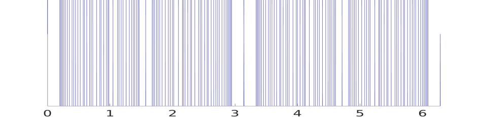
Of course the points whose angular difference is a rational number times $\pi$ form a dense set so at face value this might seem a mathematical, but certainly not a practical, condition. However, from the above argument, we cannot use but a relatively small number of eigenfunctions and so the set of points $(\theta_{1},\theta_{2})$ with $\theta_{1}-\theta_{2}\neq(j/k)\pi$ for sufficiently small $k$ might have distinct intervals of sufficient length for this criteria to be quite practical. To see this, consider the rational points generated modulo $\pi$ with denominator less than the prime value $29$, that is, we are looking for rational numbers in lowest form $a/b$ with $b<29$ and checking for zeros of $\sin(a\pi/b)$ for a given $b$. Clearly taking $b=4$ gives a zero at $\theta=\pi/4$ and we must check those combinations $a/b$ that would provide a zero close to but less than $1/4$. We need only check primes $b$ in the range $2<b<29$ and the fraction closest to $1/4$ occurs at $a/b=4/17$ which is approximately $0.235$. Thus the interval that is zero free under this range of $b$ has length $0.015\pi$ radians or approximately $2.7$ degrees of arc length. Similar intervals occur at several points throughout the circle. The gaps in such a situation with $b<29$ is shown in Figure (1).

Figure 1: Gaps between angles.

Now the question is: if we restrict the eigenvalue index $k$ to be less than $29$ what range of $m$ index to we obtain and what is the lowest eigenvalue that exceeds this $k$-range? Since the $m$-index grows faster than the $k$ for a given eigenvalue index, we obtain several thousand eigenvalues, the largest being approximately $3.5\times 10^{4}$. Only with exceedingly small initial time steps we could get such an eigenvalue and its attendant eigenfunction be utilized in the computations. If we restrict $k<17$ then the zero-free interval becomes $(\pi/4,4\pi/13)$ with length approximately $10.4$ degrees and the largest eigenvalue obtained is about $1.5\times 10^{4}$. If we decrease down to $k\leq 10$ we get an angle range of $15.8$ degrees in which to work.

Thus in short, the ill-conditioning of the problem is substantially due to other factors and not to impossible restrictions on the choice of observation points $\{\theta_{\ell}\}$.

4.3 Numerical experiments

First we consider the experiment $(e1)$,

$$(e1): T=1,\ \theta_{1}=0,\ \theta_{2}=\frac{13}{32}\pi,$$

$$p(r,\theta)=\frac{5}{\sqrt{30}}\omega_{1}J_{m(1)}(\sqrt{\lambda_{1}}r)\cos{(m(1)\theta)}+\frac{2}{\sqrt{30}}\omega_{2}J_{m(2)}(\sqrt{\lambda_{2}}r)\cos{(m(2)\theta)}$$

$$\qquad\quad\quad+\frac{1}{\sqrt{30}}\omega_{2}J_{m(2)}(\sqrt{\lambda_{2}}r)\sin{(m(2)\theta)},$$

$$q(t)=\chi_{{}_{[0,1/3)}}+2\chi_{{}_{[1/3,2/3)}}+1.5\chi_{{}_{[2/3,1]}}.$$

We use noise-polluted flux measurements on the boundary points at noise levels ranging from 1% to 5% and choose the time measurement step $\delta t$ to be $0.01$.

In order to avoid the loss of accuracy caused by the multiplication between $p$ and $q$, we use the normalized exact solution of $p(x)$, namely, let $\|p\|_{L^{2}(\Omega)}=1$. To achieve this setting, in the programming of iteration (17), after each iterative step, we set $p_{j}=p_{j}/\|p_{j}\|_{L^{2}(\Omega)},\ q_{j}=\|p_{j}\|_{L^{2}(\Omega)}q_{j}$. Also, the initial guess $p_{0}$ and $q_{0}$ are set as

$$p_{0}(x) \equiv 1,\ x\in\Omega,$$

$$q_{0} :=\operatorname*{arg\,min}_{q\in L^{2}[0,T]}\|F[p_{0}]q-g^{\delta}\|_{L^{2}[0,T]}^{2}+\beta_{q}\|\triangledown q\|_{L^{1}[0,T]}.$$

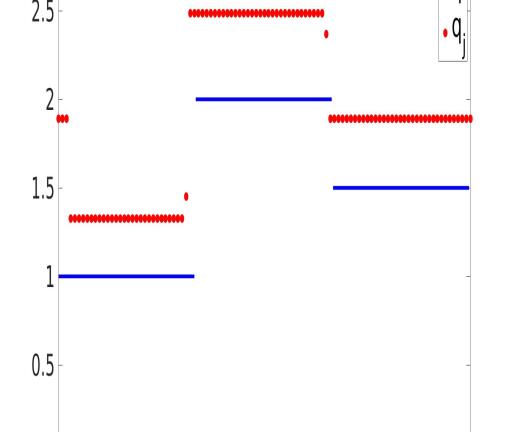
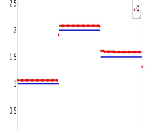
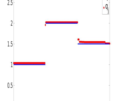
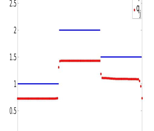
Depending on the noise level $\delta,$ the values of regularized parameters $\beta_{p}$, $\beta_{q}$ are picked empirically and here the values used are $\beta_{p}=1\times 10^{-2}$, $\beta_{q}=8\times 10^{-4}$. After $j=10$ iterations, the approximations $p_{j},q_{j}$ are recorded and displayed by Figure (2). This indicates effective numerical convergence of the scheme. The errors of approximations upon different noise levels are displayed by the following table.

	$\delta=1\%$	$\delta=3\%$	$\delta=5\%$
$\|p-p_{j}\|_{L^{2}(\Omega)}$	$1.34e-1$	$1.76e-1$	$1.87e-1$
$\|q-q_{j}\|_{L^{2}[0,T]}$	$8.08e-2$	$8.25e-2$	$9.76e-2$

The satisfactory reconstructions shown by the table confirm that the iterative scheme (17) is a feasible approach to solve this nonlinear inverse problem numerically.

   units ¡.333¿ x from 0 to 1, y from 0 to 3 bottom shiftedto y=0 ticks short numbered from 0 to 1 by 0.2 / left ticks short numbered from 0 to 3 by 1 / 0.7pt from 0 1 to 0.333 1 ¡3pt¿ t 0 0.98232 0.01 0.98232 0.02 0.98232 0.03 0.98232 0.04 0.98232 0.05 0.98232 0.06 0.98232 0.07 0.98232 0.08 0.98232 0.09 0.98232 0.1 0.98232 0.11 0.98232 0.12 0.98232 0.13 0.98232 0.14 0.98232 0.15 0.98232 0.16 0.98232 0.17 0.98232 0.18 0.98232 0.19 0.98232 0.2 0.98232 0.21 0.98232 0.22 0.98232 0.23 0.98232 0.24 0.98232 0.25 0.98232 0.26 0.98232 0.27 0.98232 0.28 0.98232 0.29 0.98232 0.3 0.98232 0.31 0.98232 0.32 0.98232 0.33 1.5476 0.34 1.8951 0.35 1.8951 0.36 1.8951 0.37 1.8951 0.38 1.8951 0.39 1.8951 0.4 1.8951 0.41 1.8951 0.42 1.8951 0.43 1.8951 0.44 1.8951 0.45 1.8951 0.46 1.8951 0.47 1.8951 0.48 1.8951 0.49 1.8951 0.5 1.8951 0.51 1.8951 0.52 1.8951 0.53 1.8951 0.54 1.8951 0.55 1.8951 0.56 1.8951 0.57 1.8951 0.58 1.8951 0.59 1.8951 0.6 1.8951 0.61 1.8951 0.62 1.8951 0.63 1.8951 0.64 1.8951 0.65 1.8951 0.66 1.8951 0.67 1.8951 0.68 1.5033 0.69 1.5033 0.7 1.5033 0.71 1.5033 0.72 1.5033 0.73 1.5033 0.74 1.5033 0.75 1.5033 0.76 1.5033 0.77 1.5033 0.78 1.5033 0.79 1.5033 0.8 1.5033 0.81 1.5033 0.82 1.4962 0.83 1.4962 0.84 1.4962 0.85 1.4962 0.86 1.4962 0.87 1.4962 0.88 1.4817 0.89 1.4817 0.9 1.4817 0.91 1.4816 0.92 1.4816 0.93 1.4816 0.94 1.4816 0.95 1.4816 0.96 1.4816 0.97 1.4816 0.98 1.4816 0.99 1.4816 1 1.4816 / from 0 1 to 0.333 1 from 0.334 2 to 0.666 2 from 0.667 1.5 to 1 1.5

Figure 2: Experiment $(e1)$, $p$ (left), $p_{j}$ (center) and $q,\,q_{j}$ (right). Noise $\delta=1\%$.

Next, we seek recovery of a more general $p(x)$:

$$(e2): p(r,\theta)=\chi_{{}_{r\leq 0.5+0.2\cos{2\theta}}},$$

$$q(t)=\chi_{{}_{[0,1/3)}}+2\chi_{{}_{[1/3,2/3)}}+1.5\chi_{{}_{[2/3,1]}},$$

$$(e3): p(r,\theta)=\chi_{{}_{r\leq 0.25+0.1\cos{2\theta}}},$$

$$q(t)=\chi_{{}_{[0,1/3)}}+2\chi_{{}_{[1/3,2/3)}}+1.5\chi_{{}_{[2/3,1]}}.$$

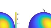
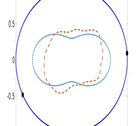
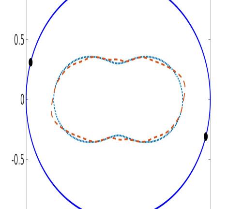
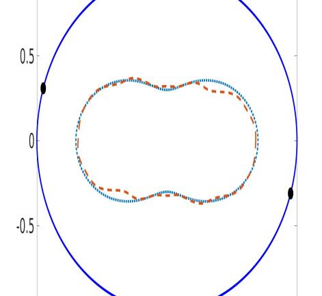
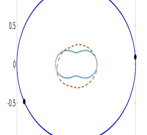
In experiment $(e2)$, a discontinuous, star-like supported exact solution $p(x)$ is considered, where the radius function is $r(\theta)=0.5+0.2\cos{2\theta}$. We can see this $p$ is out of Assumption (2.1), so the iteration (17) may not be appropriate here and in fact, we use the Levenberg–Marquardt algorithm to recover the radius function $r(\theta)$, see [11] for details. The numerical results are presented in Figures (3), (4) and (5), in which the blue dotted line and the red dashed line mean the boundaries of $\text{supp}(p)$ and $\text{supp}(p_{j})$, respectively, and the black bullets are the locations of observation points.

Figures (4) and (5) show that with sufficient data, for example, more measurement points and finer mesh on time $t$, precise reconstructions can be obtained even though Assumption (2.1) is violated. These results indicate that, if we do not pursue the global uniqueness stated by Theorem (1), which requires Assumption (2.1), the conditions on $p$ and $q$ may be weakened in numerical computations. This inspires future work on such inverse source problems in order to provide a rigorous mathematical justification for allowing such inclusions.

Figure 3: Experiment $(e2)$, $p$ (left) and $q$ (right), $\delta=1\%$.

Figure 4: Experiment $(e2)$ with $4$ measurement points, $p$ (left) and $q$ (right), $\delta=1\%$.

Figure 5: Experiment $(e2)$ with $4$ measurement points and $\delta t=5\times 10^{-3}$, $p$ (left) and $q$ (right), $\delta=1\%$.

If we use equation (1) to describe the diffusion of pollutants, then $\text{supp}(p)$ means the severely polluted area. With the consideration of safety and cost, observations of the flux data should be made as far as possible to $\text{supp}(p)$. This is the reason why we set the experiment $(e3)$, in which $p(x)$ has a smaller support. Due to the long distance between $\text{supp}(p)$ and the observation points, worse results can be expected. See Figure (6). Hence, accurate and efficient algorithms for this inverse source problem with a small $\text{supp}(p)$ are worthy of investigation. Of course, in the limit that these become point sources described by Dirac-delta functions then other tools are available. See, for example, [5].

Figure 6: Experiment $(e3)$, $p$ (left) and $q$ (right), $\delta=1\%$.

5 Concluding remark and future work

This paper considers the unique determination of a nonlinear source term in the heat equation, which contains two independent unknowns. Only finite (here is two) flux measurements are sufficient to support this uniqueness, provided some restrictions on $p,q$ stated by Assumption (2.1). Here a natural question may be asked, can we weaken the conditions on $p,q$ and meanwhile keep the uniqueness result. Let’s review the roles of such conditions in the uniqueness proof. The smoothness condition $p\in\mathcal{D}((-\Delta)^{\gamma})$ ensures Lemma (3.2), the absolute convergence of the series $\sum_{n=1}^{\infty}a_{n}(z)p_{n}$, which supports the well-definedness of the Laplace transform (12) and Lemma (3.3). While the step function form of $q$ is set for the proof of the main theorem, Theorem (1). The Laplace transform of Heaviside function is the natural exponential function, which can not be factored with rational functions, i.e. $a_{n}(z)p_{n}\lambda_{n}(s+\lambda_{n})^{-1}$. This means we can isolate each coefficient pair $(q_{k},c_{k})$ of $q$ with others in the uniqueness proof and then deduce the uniqueness result $p(x)=C_{0}\tilde{p}(x)$ for the space unknown $p$. After this step, the nonlinear inverse problem is linearized and naturally, the uniqueness of time unknown $q$ is derived. To sum up, to weaken the conditions on $p$ and $q$, a new approach may need to be constructed rather than the Laplace transform.

However, the numerical experiments $(e2)$ and $(e3)$ seem to provide a feasible way. In the numerical reconstruction aspect, we may consider more general unknowns, for instance, discontinuous $p(x)$ and even continuous $q(t)$. But in the numerical analysis, we may only prove the local uniqueness result, not the global one as Theorem (1). It may be regarded as the cost for a wider class of unknowns.

Furthermore, extending this work to fractional diffusion equations is interesting and meaningful. The fractional case to recover the space dependent source $f(x,t)=\chi_{{}_{D}}$ was considered in [11]. In the fractional diffusion equation, the regular time derivative $\partial/\partial t$ is replaced by the fractional derivative $\partial_{t}^{\alpha},\ \alpha\in(0,1).$ The fundamental solution for such equations is in terms of Mittag-Leffler function $E_{\alpha_{1},\alpha_{2}}(-z)$, but not the natural exponential function. This function also holds the analytic property, which means the uniqueness proof seems to work. Also, comparing with the natural exponential function, the polynomial decay rate of $E_{\alpha_{1},\alpha_{2}}(-z)$ may cause different performance in the numerical reconstruction. In addition, if the fractional order $\alpha$ is set to be unknown, this inverse problem will become more challenging.

References

- [1] J. R. Cannon. Determination of an unknown heat source from overspecified boundary data source in the heat equation. SIAM Journal on Numerical Analysis, 5(2), 1968.
- [2] J. R. Cannon and S. P. Esteva. An inverse problem for the heat equation. Inverse Problems, 2(4):395–403, nov 1986.
- [3] E. Di Nezza, G. Palatucci, and E. Valdinoci. Hitchhiker’s guide to the fractional Sobolev spaces. Bull. Sci. Math., 136(5):521–573, 2012.
- [4] D. S. Grebenkov and B.-T. Nguyen. Geometrical structure of Laplacian eigenfunctions. SIAM Rev., 55(4):601–667, 2013.
- [5] M. Hanke and W. Rundell. On rational approximation methods for inverse source problems. Inverse Probl. Imaging, 5(1):185–202, 2011.
- [6] F. Hettlich and W. Rundell. Identification of a discontinuous source in the heat equation. Inverse Problems, 17(5):1465–1482, 2001.
- [7] V. Isakov. Inverse source problems, volume 34 of Mathematical Surveys and Monographs. American Mathematical Society, Providence, RI, 1990.
- [8] J.-L. Lions and E. Magenes. Non-homogeneous boundary value problems and applications. Vol. I. Springer-Verlag, New York-Heidelberg, 1972. Translated from the French by P. Kenneth, Die Grundlehren der mathematischen Wissenschaften, Band 181.
- [9] J. L. Mueller and S. Siltanen. Linear and nonlinear inverse problems with practical applications, volume 10 of Computational Science & Engineering. Society for Industrial and Applied Mathematics (SIAM), Philadelphia, PA, 2012.
- [10] W. Rundell. An inverse problem for a parabolic partial differential equation. Rocky Mountain J. Math., 13(4):679–688, 1983.
- [11] W. Rundell and Z. Zhang. Recovering an unknown source in a fractional diffusion problem. J. Comput. Phys., 368:299–314, 2018.
- [12] C. L. Siegel. Über einige Anwendungen diophantischer Approximationen [reprint of Abhandlungen der Preußischen Akademie der Wissenschaften. Physikalisch-mathematische Klasse 1929, Nr. 1]. In On some applications of Diophantine approximations, volume 2 of Quad./Monogr., pages 81–138. Ed. Norm., Pisa, 2014.