Teaching forced damped oscillator using RLC circuit through inverse modeling

Abstract

Teaching by direct models in science has been weakening the learning process of the students, because the real problems in engineering are not solved by direct models instead commonly they are solve by inverse models. On the other hand, one of the most relevant topics in the course of waves and particle physics oriented for the forming engineers; it’s the subject of simple harmonic motion forced damping, which many physical phenomena can be explained as the quality factor Q and the resonance frequency of an oscillatory forced system. In order to capture the attention of students and give an application to this issue. We have developed an experimental setup to take measurements of electric current, voltages from capacitor and inductor for different frequencies and resistances, once the experimental data were collected to study the behavior of the electrical current inside the circuit and find out the RLC parameters with an inverse model. Finally, we want to show the process in detail how parameters of the system (Resistance, Inductance and Capacitance values) are very relevant in this kind of systems, from the results obtained by experimental measurements of voltage, current and angle of phase shift, where this was achieved by implementing an indirect method described in this document, so that can be applied to studies of more complex systems such as a motor where such parameters may be unknown.

Keywords Damped forced harmonic oscillator  $\cdot$ damped frequency  $\cdot$ forced frequency  $\cdot$ resonance frequency  $\cdot$ relaxing time  $\cdot$ quality factor Q.

1 Introduction

In many of the current works, experiments of an RLC circuit have been carried out, using numerical and experimental methods to solve the second-order differential equation that governs the behavior of the current along the electric circuit to be studied [1, 2, 3, 4, 5, 6].

It is very uncommon to find a research work, in which the students are shown the physical phenomenon of the problem being analyzed, for example the damped effect of the current in a series RLC circuit without previously knowing the values of the resistance, the inductivity of the coil and neither the capacitance of the capacitor used for this experiment.

We authors, we want to present a work in which you can visualize the wave phenomenon of the current, in an RLC circuit, in addition to how from measurements of current and voltage in it, we can see the damping behavior of the system, for which we use a very low resistance value which will allow us to observe the three regions of this system, which are: the inductive region, the resistive region and the capacitive region.

One of the details to highlight in this work, consists of being able to present an RLC circuit from the point of view of the forced oscillatory oscillatory movement, where two solutions are expected, which are: a transient (dominated principally by the factor of the amplitude of voltage of the generator of signals) and another quasistationary (which is presented by the connection of a coil, a resistance and a capacitor), from the two responses obtained (forced and damped) by the physical system studied in this article, we can obtain the values the resistance (R), the inductance (L) and the capacitance (C). For which we have developed a Script in Python, where the results of voltage and current of the system are analyzed principally.

This paper is organized as follows: Section 2, describes the Theoretical study corresponding to the calculates for the RLC circuit. In Section 3, shown the experimental procedure for the data takes. In Section 4 the results concerning to the validate of the experimentall method shown in the previous sections. Finally we present some conclusions about of this work.

2 Theoretical study

The physical model of the system under study is shown in Figure 1. Thissystem consists of an RLC circuit in series.

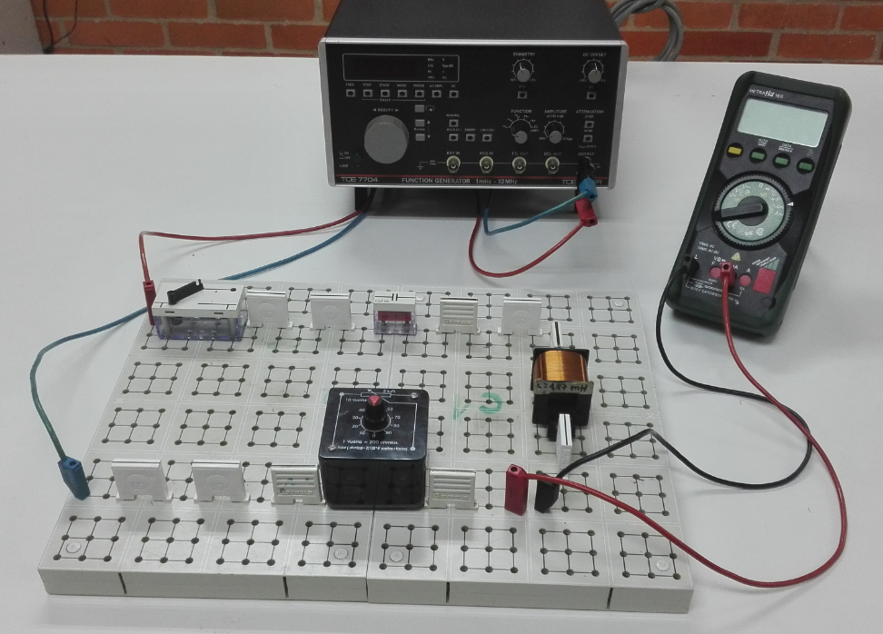
Figure 1: Experimental assembly of the RLC circuit in series.

In order to study this system, we must start with the following equation(Kirchhoff’s mesh law) [7, 8]:

$$V(t)=V_{R}(t)+V_{L}(t)+V_{c}(t)$$ (1)

$$V_{0}\sin(\omega t)=i(t)R+L\frac{di(t)}{dt}+\frac{1}{c}q(t)$$ (2)

Now using the expression of electric current as a function of charge and time, we have:

$$i(t)=\frac{dq(t)}{dt}$$ (3)

If we replace the Expression (2) in Equation (3), we obtain the following differential equation:

$$V_{0}\sin(\omega t)_{=}R\left(\frac{dq(t)}{dt}\right)+L\frac{d}{dt}\left(\frac{dq(t)}{dt}\right)+\frac{1}{c}q(t)$$ (4)

$$V_{0}\sin(\omega t)_{=}R\left(\frac{dq(t)}{dt}\right)+L\left(\frac{d^{2}q(t)}{dt^{2}}\right)+\frac{1}{c}q(t),$$ (5)

where $\omega=2\pi f$, being $f$ the temporary frequency of oscillation of the voltage source and by organizing Equation (5), we have:

$$\frac{V_{0}}{L}\sin(2\pi ft)=\frac{R}{L}\left(\frac{dq(t)}{dt}\right)+\left(\frac{d^{2}q(t)}{dt^{2}}\right)+\frac{1}{LC}\left(q(t)\right)$$ (6)

$$\frac{V_{0}}{L}\sin(2\pi ft)=\left(\frac{d^{2}q(t)}{dt^{2}}\right)+\frac{R}{L}\left(\frac{dq(t)}{dt}\right)+\frac{1}{LC}\left(q(t)\right)$$ (7)

From Equation (7), and using the equation of a forced and damped harmonic oscillator, we can write [9, 10]:

$$F_{0}\sin(2\pi ft)=\left(\frac{d^{2}x(t)}{dt^{2}}\right)+\gamma\left(\frac{dx(t)}{dt}\right)+\omega^{2}_{0}\left(x(t)\right),$$ (8)

where $\gamma$ is the damping factor, $F_{0}$ is the amplitude of the applied force and $\omega_{0}$ is the natural frequency of the system. Comparing Equation (7) with the expression (8), we can obtain the following expressions:

$$F_{0}=\frac{V_{0}}{L},\quad\omega_{0}=\frac{1}{\sqrt{LC}},\quad\gamma=\frac{R}{L}.$$ (9)

Given that the system current $i(t)$ (See the Figure 2) can be expressed as a function of the voltage $V(t)$ using the following equations,

$$i(t)=\frac{V(t)}{Z(w)}=\frac{V(t)}{\sqrt{R^{2}+(L\omega-\frac{1}{\omega C})^{2}}},$$ (10)

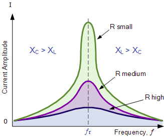
Figure 2: Graph of the current as a function of the frequency, where the expected behavior for three resistances of different values is observed.

where $z(\omega)$ is the impedance of the circuit, it should be noted that the expression to find the amount of charge stored in the circuit, we can write the harmonic relationship of the charge with the angular frequency of the system $i(t)=I_{0}\cos(\omega t+\phi)$, we have:

$$\frac{dq}{dt}=I_{0}\cos(\omega t+\phi)$$ (11)

$$\int dq=\int I_{0}\cos(\omega t+\phi)dt$$ (12)

$$q(t)=\frac{I_{0}}{\omega}\sin(\omega t+\phi)+C.$$ (13)

If we take into account only the maximum value (amplitude of the function) of the current and the charge we have:

$$I_{0}=\frac{V_{0}}{\sqrt{R^{2}+(L\omega-\frac{1}{\omega C})^{2}}},\quad Q_{0}=\frac{V_{0}}{\omega\sqrt{R^{2}+(L\omega-\frac{1}{\omega C})^{2}}}.$$ (14)

It is also of great importance to define a phase angle $\beta$ of the circuit between the voltage of the coil, that of the capacitor and that of the resistance (See the Figure 3).

$$\tan(\beta)=\frac{L\omega-\frac{1}{c\omega}}{R}.$$ (15)

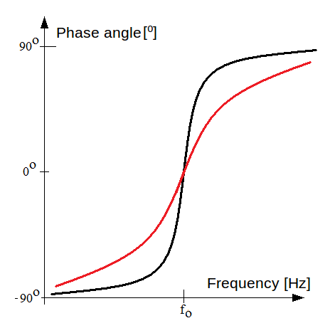
Figure 3: Beta angle behavior $\beta$ for two different resistance values in a series RLC circuit, where the black curve belongs to the value of the lowest value resistance $R_{1}$, so the curve of red color corresponds to the resistance of greater value $R_{2}$ ($R_{2}>R_{1}$).

One of the most important parameters to be calculated in this type of systems (serial RLC circuit), is the quality factor or merit factor denoted also as factor Q, is defined experimentally as:

$$Q_{exp}=\frac{\omega_{0}}{\Delta f}=\frac{f_{0}}{f_{2}-f_{1}},$$ (16)

Where $f_{0}$ is the resonance frequency of the system, in addition, we can calculate this factor theoretically through the following analytical calculation:

$$Q_{the}=\frac{\omega_{0}L}{R}=\frac{2\pi f_{0}L}{R}$$ (17)

Finally, a parameter that can give us indications of the behavior of the energy in the circuit is the average power $P_{a}$ (See the Figure 4), which is expressed as:

$$P_{a}=V_{a}\cdot I_{a}=V_{0}\cdot I_{0},$$ (18)

where $I_{a}$ and $V_{a}$ are the average value corresponding of current and voltage. Also $V_{0}$ and $I_{0}$ are the amplitude values of the voltage and current respectively.

Figure 4: Calculation of the average power of an RLC circuit for the following parameters: $C=2.0$ $nf$, $L=5.0$ $\mu H$ and rms voltage of $5.0$ $mV$.

3 Experimental study

We initially carried out the assembly of a series RLC circuit, with the values of resistance R, inductance L and capacitance C supplied. In order for the circuit to behave as forced movement, also add in series an AC source.

Where the procedure to follow is as follows:

1. For the values of $L=4,83$ $mH$ and $C=4,7$ $\mu$F given, calculate the theoretical value of the resonant frequency of the circuit, according to the Equation (9).

2. Start the data collection with a frequency of 100 Hz and measure the circuit current.

3. Increase the value of the frequency by 100 and measure again, until you find the maximum current of the circuit (in resonance).

4. From the last previous value increase the frequency of the generator in larger intervals (600 Hz) and continue measuring the current until a value close to that measured with the initial frequency of 100 Hz is obtained.

5. Vary the resistance of the potentiometer and repeat steps 3 to 5.

In Table 1, we organize the data taken from the experiment, where we can see that in our case we have a resonance frequency $f_{0}=1044$ $Hz$.

f [Hz]	I (R = 6 $\Omega$) [mA]	I (R = 20 $\Omega$) [mA]	I (R = 50 $\Omega$) [mA]	I (R = 100 $\Omega$) [mA]
100	5,32	5,27	5,16	4,91
200	10,38	10,01	9,24	7,99
300	14,85	13,88	12,05	9,57
400	18,66	16,89	13,82	10,4
500	21,72	19,09	14,95	10,85
600	24,1	20,63	15,66	11,11
700	25,77	21,67	16,1	11,26
800	26,91	22,32	16,35	11,34
900	27,6	22,69	16,5	11,39
1000	27,82	22,85	16,55	11,4
1044	27,84	22,86	16,6	11,402
1200	27,61	22,72	16,5	11,38
1800	24,29	20,72	15,69	11,1
2400	20,54	18,26	14,52	10,66
3000	17,43	15,97	13,28	10,13
3600	15,04	14,07	12,12	9,58
4200	13,18	12,5	11,07	9,03
5400	10,49	11,2	10,13	8,49
6000	9,5	10,12	9,32	7,99
6600	8,67	9,23	8,6	7,52
7200	7,96	8,47	8	7,1
8000	7,18	7,83	7,42	6,7
8400	6,86	7,25	6,92	6,32
9000	6,41	6,76	6,49	5,98
9600	5,99	6,33	5,75	5,67
10200	5,66	5,95	5,45	5,13
10860	5,32	5,27	5,16	4,91

Table 1: Experimental data taken from the RLC circuit current in series, for four different resistance values.

4 Results

Once we take the experimental data of the current in the series RLC circuit, using equation (15), we can obtain the value of the phase angle for the charge $\alpha=-\beta$ and the angular shift of the current $\beta$. In Table 2, we calculate the value of the phase angle $\alpha$ and $\beta$, for the charge and the current respectively, as a function of the temporal oscillation frequency of the source using the electric signal generator.

It is important to note that in Table 2, we have performed the calculation of the $\alpha$ and $\beta$ phase angle with the same frequency intervals for values below the resonant frequency $f_{0}$ (Capacitive regime) and for values above the resonant frequency $f_{0}$ (Inductive regime).

f [Hz]	$\alpha$ [0] ($R=6$ $\Omega$)	$\beta$ [0] ($R=6$ $\Omega$)	$\alpha$ [0] ($R=20$ $\Omega$)	$\beta$ [0] ($R=20$ $\Omega$)
100	88,975728634	-88,975728634	86,5894322956	-86,5894322956
200	87,895055545	-87,895055545	83,0151690125	-83,0151690125
300	86,69088025	-86,69088025	79,0910790978	-79,0910790978
400	85,2702154409	-85,2702154409	74,5814380592	-74,5814380592
500	83,4865468164	-83,4865468164	69,1642654147	-69,1642654147
600	81,0803124717	-81,0803124717	62,3832531777	-62,3832531777
700	77,5301965014	-77,5301965014	53,6046128861	-53,6046128861
800	71,6128821857	-71,6128821857	42,0665903255	-42,0665903255
900	59,8078349139	-59,8078349139	27,2762553702	-27,2762553702
1000	30,3629721352	-30,3629721352	9,9678484578	-9,9678484578
1044	7,1485248931	-7,1485248931	2,1547384631	-2,1547384631
1200	-53,8013992912	53,8013992912	-22,2896571884	22,2896571884
1800	-80,4892669759	80,4892669759	-60,8187979584	60,8187979584
2400	-84,1662882661	84,1662882661	-71,192734547	71,192734547
3000	-85,69776159	85,69776159	-75,9224811181	75,9224811181
3600	-86,5610762758	86,5610762758	-78,6730414637	78,6730414637
4200	-87,123190111	87,123190111	-80,4908489724	80,4908489724
5400	-87,8198404866	87,8198404866	-82,7679463229	82,7679463229
6000	-88,0523884798	88,0523884798	-83,5330624823	83,5330624823
6600	-88,2390949738	88,2390949738	-84,1488928557	84,1488928557
7200	-88,3925021602	88,3925021602	-84,6558196597	84,6558196597
8000	-88,5591992297	88,5591992297	-85,2075262198	85,2075262198
8400	-88,6300410296	88,6300410296	-85,4422377182	85,4422377182
9000	-88,7239819496	88,7239819496	-85,7536946762	85,7536946762
9600	-88,80572858	88,80572858	-86,0249087976	86,0249087976
10200	-88,8775316953	88,8775316953	-86,2632672432	86,2632672432
10860	-88,9470770968	88,9470770968	-86,4942434092	86,4942434092

Table 2: Values of the phase angles $\alpha$ $\beta$ of the charge and current of the RLC circuit as a function of the frequency $f$ for the values of resistance $R=6$ $\Omega$ and $R=20$ $\Omega$.

In order to compare the behavior of the phase angle $\alpha$ and $\beta$ for the four different resistance values taken in this experiment ($R=10,20,50$ and $100$ $\Omega$), we show in Table 3, the phase angles for the charge and the current taking into account the highest value of the resistors.

f [Hz]	$\alpha$ [0] ($R=50$ $\Omega$)	$\beta$ [0] ($R=50$ $\Omega$)	$\alpha$ [0] ($R=100$ $\Omega$)	$\beta$ [0] ($R=100$ $\Omega$)
100	81,5258323067	-81,5258323067	73,4069850003	-73,4069850003
200	72,9707197615	-72,9707197615	58,5092331715	-58,5092331715
300	64,2739395152	-64,2739395152	46,0603394561	-46,0603394561
400	55,4142738385	-55,4142738385	35,948785169	-35,948785169
500	46,4252981071	-46,4252981071	27,72265128	-27,72265128
600	37,4009875007	-37,4009875007	20,9214813894	-20,9214813894
700	28,485951325	-28,485951325	15,179996904	-15,179996904
800	19,8497996067	-19,8497996067	10,2318390307	-10,2318390307
900	11,6535938515	-11,6535938515	5,8876870228	-5,8876870228
1000	4,0212419436	-4,0212419436	2,0130999935	-2,0130999935
1044	0,8622368479	-0,8622368479	0,431142834	-0,431142834
1200	-9,3117916954	9,3117916954	-4,6868441384	4,6868441384
1800	-35,6127922537	35,6127922537	-19,7041583231	19,7041583231
2400	-49,5881568393	49,5881568393	-30,4236726718	30,4236726718
3000	-57,9158297186	57,9158297186	-38,5743814181	38,5743814181
3600	-63,3995434547	63,3995434547	-44,9557637943	44,9557637943
4200	-67,2776729403	67,2776729403	-50,0526808255	50,0526808255
5400	-72,3986576007	72,3986576007	-57,6053246212	57,6053246212
6000	-74,1784494296	74,1784494296	-60,4573638028	60,4573638028
6600	-75,630236387	75,630236387	-62,8699498965	62,8699498965
7200	-76,8372303376	76,8372303376	-64,9333375978	64,9333375978
8000	-78,1621641571	78,1621641571	-67,2565532532	67,2565532532
8400	-78,7291642709	78,7291642709	-68,2687197496	68,2687197496
9000	-79,4844382998	79,4844382998	-69,6330607008	69,6330607008
9600	-80,144656899	80,144656899	-70,840227315	70,840227315
10200	-80,7267296339	80,7267296339	-71,9153140726	71,9153140726
10860	-81,2923208693	81,2923208693	-72,9692652491	72,9692652491

Table 3: Values of the phase angles $\alpha$ $\beta$ of the charge and current of the RLC circuit as a function of the frequency $f$ for the values of resistance $R=50$ $\Omega$ and $R=100$ $\Omega$.

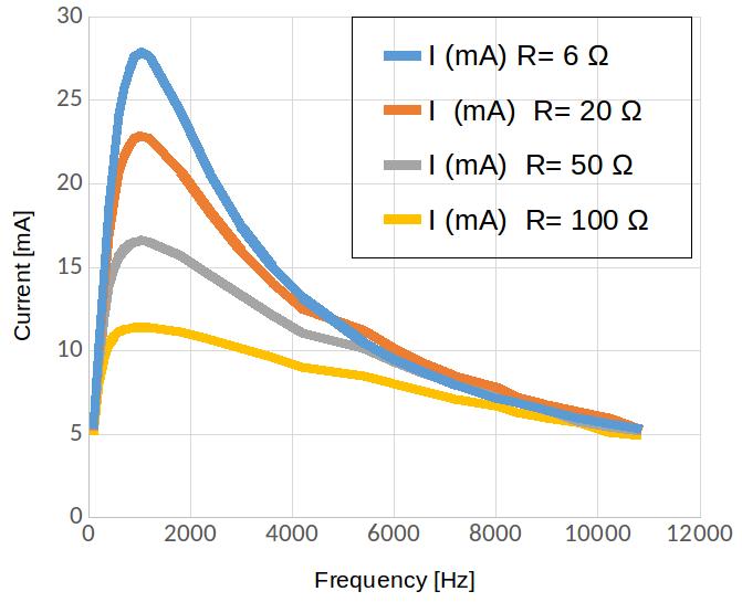
Figure 5: Graph of the current as a function of the frequency of the RLC circuit in series for four different resistance values.

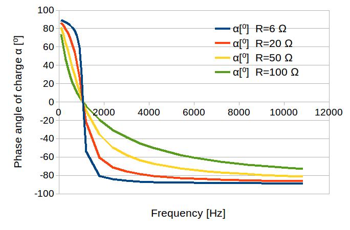
Figure 6: Phase angle of the electric charge, stored in the RLC circuit in series as a function of the frequency for four different resistance values.

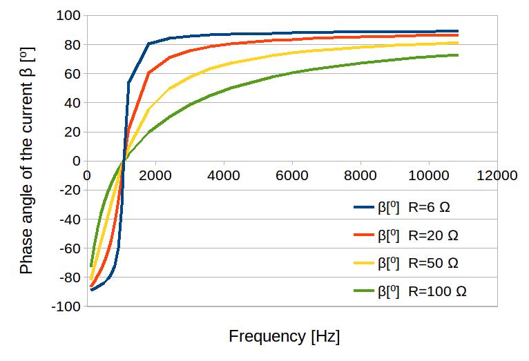
Figure 7: Phase angle of the electric current, circulating in the RLC circuit in series as a function of the frequency for four different resistance values.

In Figure 5, we show the current curves for the four resistance values that we work in this article, where you can notice the behavior of the current as a function of the frequency, where you can also see the more damped behavior (curve with lower height) to in the case of the higher value resistors ($R=50$ and $100$ $\Omega$) and, on the contrary, a behavior with a lower damping factor in the case of lower value resistors ($R=6$ and $20$ $\Omega$), this result corresponds to analytical way with Equation (9).

In Figure 6 and Figure 7, we can see the behavior of the phase angle for the electric charge and the current respectively, it should be noted that at a lower resistance value, the graphs show a more curved or smooth behavior and a more linear profile in the case of the highest resistance value.

Also, we show in table 4 the results of the experimental and theorical quality factor $Q$ (See the equations (16) and (17)) for the four resistances, based on the frequency values $f_{1}$ and $f_{2}$ using Figure 5.

R [$\Omega$]	$f_{1}$ [Hz]	$f_{2}$ [Hz]	$Q$(the)	$Q$(exp)
6	945,14	1142,9	5,247	5,279
20	713,6	1374,4	1,574	1.579
50	220,7	1867,34	0,629	0,634
100	45,7	2687,7	0,315	0,395

Table 4: Table of values of the quality factor Q, obtained experimentally and theoretically from equations (16) and (17) for the 4 different values of resistance taken in this experiment.

Finally in Table 5, we show the respective experimental errors obtained in this work.

R [$\Omega$]	Absolute error Q	Percentage relative error Q (%)
6	0,032	0,609
20	0,005	0,317
50	0,005	0,794
100	0,08	25,396

Table 5: Table of the calculation of the experimental errors for the quality factor Q for the different resistances taken into account in the experiment.

5 Conclusions

In this work the process of implementation of the study of a forced oscillatory movement has been shown in detail, using as an analogy the experimental tool of the assembly of a series RLC circuit, in which it could be seen how the capacitive and inductive region of this case differ at a factor of approximately three orders of magnitude, which is mostly due to the difference in values between the capacitor and the coil used for the development of this article.

With this research, students could be shown a practical example in which the damping factor is involved with the value of the resistance taken in the series RLC circuit, where the relationship between the damping factor and the resistance It is directly proportional, in addition to being able to experimentally observe the value of the resonant frequency in the system for the maximum current amplitude obtained experimentally.

Finally, in this document it was possible to calculate the respective experimental errors obtained for the quality factor Q depending on the value of the resistance taken, where quite acceptable values were obtained.

References

- [1] Pershin, Y. V., La Fontaine, S., & Di Ventra, M. (2009). Memristive model of amoeba learning. Physical Review E, 80(2), 021926.
- [2] Comi, C., Corigliano, A., Langfelder, G., Longoni, A., Tocchio, A., & Simoni, B. (2010). A resonant microaccelerometer with high sensitivity operating in an oscillating circuit. Journal of microelectromechanical systems, 19(5), 1140-1152.
- [3] Flanagan, J., & Landgraf, L. (1968). Self-oscillating source for vocal-tract synthesizers. IEEE Transactions on Audio and Electroacoustics, 16(1), 57-64.
- [4] Ibrahim, D. (2011). Engineering simulation with MATLAB: improving teaching and learning effectiveness. Procedia Computer Science, 3, 853-858.
- [5] Herniter, M., Scott, D., & Pangasa, R. (2001). Teaching programming skills with MATLAB. age, 6, 1.
- [6] Kofman, H. A., & Concari, S. B. (2012). Using remote lab for physics teaching. J. García Zubía, & G. Alves (comp.), Using remote labs in education, 293-308.
- [7] Sears, Z. (1976). Young, University Physics.
- [8] Serway, R. A., Jewett, J. W., Hernández, A. E. G., & López, E. F. (2005). Física para ciencias e ingeniería (Vol. 6). Thomson.
- [9] Zill, D., Wright, W. S., & Cullen, M. R. (2011). Advanced engineering mathematics. Jones & Bartlett Learning.
- [10] Tipler, P. A., & Mosca, G. (2007). Physics for scientists and engineers. Macmillan.