A gPAV-Based Unconditionally Energy-Stable Scheme for Incompressible Flows with Outflow/Open Boundaries

Abstract

We present an unconditionally energy-stable scheme for approximating the incompressible Navier-Stokes equations on domains with outflow/open boundaries. The scheme combines the generalized Positive Auxiliary Variable (gPAV) approach and a rotational velocity-correction type strategy, and the adoption of the auxiliary variable simplifies the numerical treatment for the open boundary conditions. The discrete energy stability of the proposed scheme has been proven, irrespective of the time step sizes. Within each time step the scheme entails the computation of two velocity fields and two pressure fields, by solving an individual de-coupled Helmholtz (including Poisson) type equation with a constant pre-computable coefficient matrix for each of these field variables. The auxiliary variable, being a scalar number, is given by a well-defined explicit formula within a time step, which ensures the positivity of its computed values. Extensive numerical experiments with several flows involving outflow/open boundaries in regimes where the backflow instability becomes severe have been presented to test the performance of the proposed method and to demonstrate its stability at large time step sizes.

Keywords: energy stability; unconditional stability; auxiliary variable; generalized positive auxiliary variable; open boundary condition; outflow

1 Introduction

This work concerns the numerical approximation and computation of incompressible flows on domains with outflow or open boundaries. The presence of the outflow/open boundary significantly escalates the challenge for incompressible flow simulations. A well-known issue is the so-called backflow instability Dong2015clesobc ; DongS2015 , which refers to the numerical instability associated with strong vortices or backflows at the outflow/open boundary and can cause the simulation to instantly blow up at moderate or high Reynolds numbers. The boundary condition imposed on the outflow/open boundary plays a critical role in the stability of such simulations. In the past few years a class of effective methods, so-called energy-stable open boundary conditions DongKC2014 ; DongS2015 ; Dong2015clesobc ; NiYD2019 , have been developed and can effectively overcome the backflow instability; see also related works in BruneauF1994 ; BruneauF1996 ; BazilevsGHMZ2009 ; Moghadametal2011 ; PorporaZVP2012 ; GravemeierCYIW2012 ; BertoglioC2014 ; IsmailGCW2014 ; BertoglioC2016 , among others.

In the current work we focus on the numerical approximation of the incompressible Navier-Stokes equations together with the energy-stable open boundary conditions (ESOBC), and propose an unconditionally energy-stable scheme for such problems. Two important issues are encountered immediately, which call for some comments here. First, the inclusion of ESOBC, which is nonlinear in nature Dong2015clesobc , makes the numerical approximation of the system and the proof of discrete energy stability considerably more challenging. Second, the computational cost per time step of energy-stable schemes is an issue we are conscious of. The goal here is to develop discretely energy-stable schemes with a relatively low computational cost, so that they can be computationally competitive and efficient even on a per-time-step basis.

There is a large volume of literature on the numerical schemes for incompressible Navier-Stokes equations (absence of open/outflow boundaries); see the reviews Gresho1991 ; GuermondMS2006 . These schemes can be broadly classified into two categories: semi-implicit splitting type schemes and unconditionally energy-stable schemes. The semi-implicit or fractional-step schemes (see e.g. Chorin1968 ; Temam1969 ; KimM1985 ; KarniadakisIO1991 ; BrownCM2001 ; XuP2001 ; GuermondS2003 ; LiuLP2007 ; HyoungsuK2011 ; SersonMS2016 , among others) typically treat the nonlinear term explicitly and de-couple the computations for the flow variables (pressure/velocity) by a splitting strategy. These schemes have a low computational cost per time step, because the coefficient matrices involved therein are all constant and can be pre-computed. The main drawback of these schemes lies in their conditional stability, and the computation is stable only when the time step size is sufficiently small. Thanks to their low cost, such schemes have been widely used in the simulations of turbulence and flow physics studies of single- and multi-phase problems; see e.g. KravchenkoM2000 ; DongKER2006 ; VargheseFF2007 ; Dong2009 ; GhaisasSF2015 ; SaudRT2017 ; Dong2017 ; LeeRA2017 . In the presence of outflow/open boundaries, the numerical methods employed in DongKC2014 ; Dong2014obc ; DongS2015 ; Dong2015clesobc ; DongW2016 ; NiYD2019 also belong to the semi-implicit type schemes. The unconditionally energy-stable schemes (see e.g. Shen1992 ; SimoA1994 ; VerstappenV2003 ; GuermondMS2005 ; LabovskyLMNR2009 ; DongS2010 ; Sanderse2013 ; JiangMRT2016 ; ChenSZ2018 , among others) typically treat the nonlinear term in a fully implicit or linearized fashion, and can alleviate or eliminate the constraint on the time step size encountered with semi-implicit schemes. The main drawback of energy-stable schemes lies in that they typically require the solution of a system of nonlinear algebraic equations or a system of linear algebraic equations with a variable and time-dependent coefficient matrix within a time step DongS2010 . Their computational cost per time step is quite high due to the Newton type nonlinear iterations and/or the need for frequent re-computations of the coefficient matrices (every time step).

Mindful of the strengths and weaknesses of traditional energy-stable algorithms as discussed above, in this paper we propose a new unconditionally energy-stable scheme for the incompressible Navier-Stokes equations together with the convective-like energy-stable open boundary conditions from Dong2015clesobc . This scheme in some sense combines the strengths of semi-implicit schemes and the traditional energy-stable schemes. A prominent feature lies in that, while being unconditionally energy-stable, within a time step it requires only the solution of de-coupled linear algebraic systems with constant coefficient matrices that can be pre-computed. As a result, the scheme is computationally very competitive and efficient. The unconditional discrete energy stability has been proven in the presence of outflow/open boundaries, regardless of the time step sizes.

These attractive properties of the proposed scheme are achieved by the use of an auxiliary variable associated with the total energy of the Navier-Stokes system. Such an auxiliary variable was introduced in a very recent work LinYD2019 for the incompressible Navier-Stokes equations (see also ShenXY2018 ; YangLD2019 ; YangD2019twop for related problems). The adoption of the auxiliary variable enables us to deal with the ESOBC in a relatively simple way. It should be noted that the auxiliary variable and the Navier-Stokes equations are treated in a very different way in the current work than in LinYD2019 . In this work the incompressible Navier-Stokes equations, the dynamic equation for the auxiliary variable, and the energy-stable open boundary conditions have been reformulated based on the generalized Positive Auxiliary Variable (gPAV) approach. The gPAV approach is originally developed in YangD2019diss for general dissipative systems, and provides a systematic procedure for treating dissipative partial differential equations.

We treat the gPAV-reformulated system of equations numerically in a judicious way to arrive at a discrete scheme for simulating incompressible flows with outflow/open boundaries. The scheme incorporates features of the rotational velocity-correction type strategy that is reminiscent of semi-implicit type algorithms (see e.g. GuermondMS2006 ; DongKC2014 ; DongS2012 ; Dong2014obc ; Dong2014 ). The unconditional energy stability of this scheme is proven. We show that within each time step the scheme entails the computation of two velocity fields and two pressure fields, by solving an individual de-coupled linear equation involving a constant coefficient matrix that can be pre-computed for each of these field variables. On the other hand, the auxiliary variable (a scalar number) is computed by a well-defined explicit formula. No nonlinear algebraic solver is involved in the current scheme, and furthermore the existence and positivity of the computed auxiliary variable are guaranteed (or preserved). Note that this is in sharp contrast with the method of LinYD2019 , in which Newton-type nonlinear solvers are required for computing the auxiliary variable and neither the existence nor the positivity of the computed auxiliary variable is guaranteed.

The contribution of this paper lies in the unconditionally energy-stable scheme developed herein for simulating incompressible flows with outflow/open boundaries. The discrete formulation of the current algorithm, barring the auxiliary variable, resembles the conventional rotational velocity-correction scheme to a certain degree. In such a sense, the current algorithm can be considered as a modified velocity-correction type scheme, which turns out to be unconditionally energy-stable. By contrast, the conventional velocity-correction scheme is only conditionally stable. To the best of the authors’ knowledge, this is the first time when a rotational “velocity-correction” scheme has been proven to be unconditionally stable.

The proposed scheme is implemented using the high-order spectral element method SherwinK1995 ; KarniadakisS2005 ; ZhengD2011 ; ChenSX2012 in the current paper. It should be noted that the use of spectral elements is not essential to the current scheme, and other spatial discertization methods can equally be used in the implementation. A number of flow problems involving outflow/open boundaries, and in regimes where the backflow instability becomes a severe issue for conventional methods, have been used to demonstrate the performance of the method and its stability at large time step sizes.

The rest of this paper is structured as follows. In Section 2 we introduce an auxiliary variable defined based on the sum of the total system energy and the energy integral on the outflow/open boundary and introduce its dynamic equation. We then reformulate the governing equations together with the energy-stable open boundary condition into an equivalent system utilizing the gPAV approach. The algorithmic formulation of the scheme is then presented, and we prove its discrete energy stability property. The implementation of the scheme is also discussed in some detail. In Section 3 we use manufactured analytic solutions to demonstrate the convergence rates of the proposed scheme, and use several flow problems involving outflow/open boundaries to test the performance and demonstrate the stability of the presented method. Section 4 then concludes the discussions by some closing remarks.

2 Discretely Energy-Stable Scheme for Incompressible Flows with Open Boundaries

2.1 Incompressible Navier-Stokes Equations and Energy-Stable Open Boundary Condition

Consider a domain $\Omega$ in two or three dimensions, whose boundary is denoted by $\partial\Omega$, and an incompressible flow contained in this domain. The dynamics is described by the incompressible Navier-Stokes equations, in non-dimensional form, given by

$$\frac{\partial\mathbf{u}}{\partial t}+\mathbf{N}(\mathbf{u})+\nabla p-\nu\nabla^{2}\mathbf{u}=\mathbf{f},$$ (1a)

$$\nabla\cdot\mathbf{u}=0,$$ (1b)

where $\mathbf{u}(\mathbf{x},t)$ and $p(\mathbf{x},t)$ are the velocity and pressure, respectively, $\mathbf{N}(\mathbf{u})=\mathbf{u}\cdot\nabla\mathbf{u}$, $\mathbf{f}(\mathbf{x},t)$ is an external body force, and $\mathbf{x}$ and $t$ denote the spatial coordinate and time. $\nu$ is the non-dimensional viscosity (reciprocal of the Reynolds number $Re$),

$$\nu=\frac{1}{Re}=\frac{\nu_{f}}{U_{0}L},$$ (2)

where $\nu_{f}$ is the kinematic viscosity of the fluid, and $U_{0}$ and $L$ are the characteristic velocity and length scales.

We assume that two types of boundaries (non-overlapping) may exist in the system: Dirichlet boundary $\partial\Omega_{d}$ and open boundary $\partial\Omega_{o}$, namely, $\partial\Omega=\partial\Omega_{d}\cup\partial\Omega_{o}$. On the Dirichlet boundary the velocity distribution is known,

$$\mathbf{u}=\mathbf{w}(\mathbf{x},t),\quad\text{on}\ \partial\Omega_{d},$$ (3)

where $\mathbf{w}$ is the boundary velocity.

On the open boundary $\partial\Omega_{o}$ neither the velocity nor the pressure is known. However, we assume that in general an external boundary force, in the form of a pressure head, denoted by $p_{0}$, may be imposed on $\partial\Omega_{o}$. For domains with multiple openings (outlets/inlets), it is assumed that the imposed external pressure heads on these openings may be different. To fix the boundary condition for $\partial\Omega_{o}$, we consider the energy balance equation for the system consisting of (1a)–(1b),

$$\begin{split}\frac{\partial}{\partial t}\int_{\Omega}\frac{1}{2}|\mathbf{u}|^{2}d\Omega&=-\nu\int_{\Omega}\|\nabla\mathbf{u}\|^{2}d\Omega+\int_{\Omega}\mathbf{f}\cdot\mathbf{u}d\Omega+\int_{\partial\Omega}\left[-p\mathbf{n}\cdot\mathbf{u}+\nu\mathbf{n}\cdot\nabla\mathbf{u}\cdot\mathbf{u}-\frac{1}{2}(\mathbf{n}\cdot\mathbf{u})|\mathbf{u}|^{2}\right]dA\\ &=-\nu\int_{\Omega}\|\nabla\mathbf{u}\|^{2}d\Omega+\int_{\Omega}\mathbf{f}\cdot\mathbf{u}d\Omega+\int_{\partial\Omega_{d}}\left(-p\mathbf{n}+\nu\mathbf{n}\cdot\nabla\mathbf{u}-\frac{1}{2}(\mathbf{n}\cdot\mathbf{w})\mathbf{w}\right)\cdot\mathbf{w}dA\\ &\quad+\int_{\partial\Omega_{o}}\left[-(p-p_{0}(\mathbf{x},t))\mathbf{n}+\nu\mathbf{n}\cdot\nabla\mathbf{u}-\frac{1}{2}(\mathbf{n}\cdot\mathbf{u})\mathbf{u}\right]\cdot\mathbf{u}dA-\int_{\partial\Omega_{o}}p_{0}(\mathbf{x},t)\mathbf{n}\cdot\mathbf{u}dA,\end{split}$$ (4)

where $\mathbf{n}$ is the outward-pointing unit vector normal to $\partial\Omega$, $\|\nabla\mathbf{u}\|^{2}=\sum_{i,j=1}^{d_{im}}\partial_{i}u_{j}\partial_{i}u_{j}$ ($d_{im}$ denoting the spatial dimension), and $p_{0}(\mathbf{x},t)$ is the imposed external pressure force on $\partial\Omega_{o}$, which in general can be a distribution. Following Dong2015clesobc , we consider the following convective-like boundary condition for the open boundary $\partial\Omega_{o}$ in this work,

$$\nu D_{0}\frac{\partial\mathbf{u}}{\partial t}-(p-p_{0}(\mathbf{x},t))\mathbf{n}+\nu\mathbf{n}\cdot\nabla\mathbf{u}-\mathbf{H}(\mathbf{n},\mathbf{u})=\mathbf{f}_{b}(\mathbf{x},t),\quad\text{on}\ \partial\Omega_{o},$$ (5)

where the constant $D_{0}\geqslant 0$ represents the inverse of a convection-velocity scale on $\partial\Omega_{o}$ (see Dong2015clesobc for details), $\mathbf{f}_{b}$ is a prescribed source term for the purpose of numerical testing only and will be set to $\mathbf{f}_{b}=0$ in actual simulations. $\mathbf{H}(\mathbf{n},\mathbf{u})$ is given by Dong2015clesobc ,

$$\mathbf{H}(\mathbf{n},\mathbf{u})=\left[\frac{1}{2}|\mathbf{u}|^{2}\mathbf{n}+\frac{1}{2}(\mathbf{n}\cdot\mathbf{u})\mathbf{u}\right]\Theta_{0}(\mathbf{n},\mathbf{u}),\quad\Theta_{0}(\mathbf{n},\mathbf{u})=\frac{1}{2}\left(1-\tanh\frac{\mathbf{n}\cdot\mathbf{u}}{U_{0}\delta}\right),$$ (6)

where $\Theta_{0}$ represents a smoothed step function, taking essentially the unit value when $\mathbf{n}\cdot\mathbf{u}<0$ and vanishing otherwise. The small constant $\delta>0$ controls the sharpness of the step, and as $\delta\rightarrow 0$ the function becomes sharper and $\Theta_{0}$ approaches the step function. The boundary condition (5) (with $\mathbf{f}_{b}=0$ and $\delta$ sufficiently small) is an energy-stable boundary condition for $\partial\Omega_{o}$, in the sense that in the absence of the external forces ($\mathbf{f}=0$, $p_{0}=0$) and with zero boundary velocity ($\mathbf{w}=0$) on $\partial\Omega_{d}$ this boundary condition ensures that a modified energy of the system will not increase over time. This is because in this case the energy balance equation (4) is reduced to

$$\frac{\partial}{\partial t}\left(\int_{\Omega}\frac{1}{2}|\mathbf{u}|^{2}d\Omega+\nu D_{0}\int_{\partial\Omega_{o}}\frac{1}{2}|\mathbf{u}|^{2}dA\right)=-\nu\int_{\Omega}\|\nabla\mathbf{u}\|^{2}d\Omega-\int_{\partial\Omega_{o}}\frac{1}{2}|\mathbf{u}|^{2}|\mathbf{n}\cdot\mathbf{u}|dA,\quad\text{as}\ \delta\rightarrow 0.$$ (7)

Remark 2.1.

The following more general form for $\mathbf{H}(\mathbf{n},\mathbf{u})$ is provided in Dong2015clesobc ,

$$\mathbf{H}(\mathbf{n},\mathbf{u})=\left[(\theta+\alpha_{2})\frac{1}{2}(\mathbf{u}\cdot\mathbf{u})\mathbf{n}+(1-\theta+\alpha_{1})\frac{1}{2}(\mathbf{n}\cdot\mathbf{u})\mathbf{u}\right]\Theta_{0}(\mathbf{n},\mathbf{u}),$$ (8)

where $\theta$, $\alpha_{1}$ and $\alpha_{2}$ are constants satisfying the conditions $0\leqslant\theta\leqslant 1$, $\alpha_{1}\geqslant 0$ and $\alpha_{2}\geqslant 0$. This form also ensures that the condition given by (5) is an energy-stable boundary condition for $\partial\Omega_{o}$.

The system of equations (1a)–(1b) is supplemented by the following initial condition for the velocity,

$$\mathbf{u}(\mathbf{x},0)=\mathbf{u}_{in}(\mathbf{x}),$$ (9)

where $\mathbf{u}_{in}$ denotes the initial velocity distribution that satisfies (1b) and is compatible with the boundary condition (3) on $\partial\Omega_{d}$.

2.2 Reformulated Equivalent System

To facilitate the development of numerical algorithms we will first reformulate the system consisting of equations (1a)–(1b), the boundary conditions (3) and (5), and the initial condition (9) into an equivalent system.

Define a biased modified energy,

$$E(t)=E[\mathbf{u}]=\int_{\Omega}\frac{1}{2}|\mathbf{u}|^{2}d\Omega+\nu D_{0}\int_{\partial\Omega_{o}}\frac{1}{2}|\mathbf{u}|^{2}dA+C_{0},$$ (10)

where $C_{0}$ is a chosen energy constant that ensures $E(t)>0$ for all $t\geqslant 0$. Define an auxiliary variable $R(t)$ based on $E(t)$,

$$\left\{\begin{split}&R(t)=\sqrt{E(t)},\\ &E(t)=R^{2}(t).\end{split}\right.$$ (11)

Then $R(t)$ satisfies the following dynamic equation,

$$2R\frac{dR}{dt}=\int_{\Omega}\mathbf{u}\cdot\frac{\partial\mathbf{u}}{\partial t}d\Omega+\nu D_{0}\int_{\partial\Omega_{o}}\mathbf{u}\cdot\frac{\partial\mathbf{u}}{\partial t}dA.$$ (12)

Note that both $E(t)$ and $R(t)$ are scalar numbers, not field functions.

We define another function,

$$g(\chi)=\left\{\begin{array}[]{ll}\chi,&\text{if}\ \chi\leqslant 1,\\ 1,&\text{if}\ \chi>1.\end{array}\right.$$ (13)

Note that $\frac{R^{2}(t)}{E(t)}=1$, and so $g\left(\frac{R^{2}}{E}\right)=1$.

With the variables defined above, we reformulate equation (1a) into the following equivalent form,

$$\frac{\partial\mathbf{u}}{\partial t}+g\left(\frac{R^{2}}{E}\right)\mathbf{N}(\mathbf{u})+\nabla p-\nu\nabla^{2}\mathbf{u}=\mathbf{f}.$$ (14)

We re-write the boundary condition (5) into

$$\nu D_{0}\frac{\partial\mathbf{u}}{\partial t}-(p-p_{0})\mathbf{n}+\nu\mathbf{n}\cdot\nabla\mathbf{u}-g\left(\frac{R^{2}}{E}\right)\mathbf{H}(\mathbf{n},\mathbf{u})=\mathbf{f}_{b},\quad\text{on}\ \partial\Omega_{o}.$$ (15)

Let $\mathbf{u}_{1}$, $\mathbf{u}_{2}$, $p_{1}$, and $p_{2}$ denote four field functions that are to be specifically defined later in Section 2.4 (by equations (33)–(34) and (LABEL:equ:u1_1)–(41b)). They are related to $\mathbf{u}$ and $p$ by the relations, $\mathbf{u}=\mathbf{u}_{1}+g(\frac{R^{2}}{E})\mathbf{u}_{2}$ and $p=p_{1}+g(\frac{R^{2}}{E})p_{2}$; see equations (35) and (42) later in Section 2.4. Following the gPAV idea YangD2019diss , we incorporate the following zero terms into the right hand side (RHS) of equation (12),

$$\begin{split}&\left(\frac{R^{2}}{E}-1\right)\int_{\Omega}\left(-\nabla p+\nu\nabla^{2}\mathbf{u}\right)\cdot\mathbf{u}d\Omega+\left[g\left(\frac{R^{2}}{E}\right)-\frac{R^{2}}{E}\right]\int_{\Omega}\mathbf{N}(\mathbf{u})\cdot\mathbf{u}d\Omega\\ &+\left(\int_{\Omega}\mathbf{f}\cdot\mathbf{u}d\Omega-\int_{\Omega}\mathbf{f}\cdot\mathbf{u}d\Omega\right)+\left(\frac{R^{2}}{E}-1\right)\int_{\partial\Omega}\left(p\mathbf{n}-\nu\mathbf{n}\cdot\nabla\mathbf{u}\right)\cdot\mathbf{u}dA\\ &+\left[\frac{R^{2}}{E}-g\left(\frac{R^{2}}{E}\right)\right]\int_{\partial\Omega_{o}}\mathbf{H}(\mathbf{n},\mathbf{u})\cdot\mathbf{u}dA+\left(\int_{\partial\Omega_{o}}p_{0}\mathbf{n}\cdot\mathbf{u}dA-\int_{\partial\Omega_{o}}p_{0}\mathbf{n}\cdot\mathbf{u}dA\right)\\ &+\left(\int_{\partial\Omega_{o}}\mathbf{f}_{b}\cdot\mathbf{u}dA-\int_{\partial\Omega_{o}}\mathbf{f}_{b}\cdot\mathbf{u}dA\right)+\left(1-\frac{R^{2}}{E}\right)\int_{\partial\Omega_{d}}\left[-p\mathbf{n}+\nu\mathbf{n}\cdot\nabla\mathbf{u}-\frac{1}{2}(\mathbf{n}\cdot\mathbf{w})\mathbf{w}\right]\cdot\mathbf{w}dA\\ &+\left[\frac{R^{2}}{E}-g\left(\frac{R^{2}}{E}\right)\right]\int_{\Omega}\mathbf{f}\cdot\mathbf{u}_{2}d\Omega+\left[\frac{R^{2}}{E}-g\left(\frac{R^{2}}{E}\right)\right]\int_{\partial\Omega_{d}}\left(-p_{2}\mathbf{n}+\nu\mathbf{n}\cdot\nabla\mathbf{u}_{2}\right)\cdot\mathbf{w}dA\\ &+\left[\frac{R^{2}}{E}-g\left(\frac{R^{2}}{E}\right)\right]\int_{\partial\Omega_{o}}\left(-p_{0}\mathbf{n}\cdot\mathbf{u}_{2}+\mathbf{f}_{b}\cdot\mathbf{u}_{2}\right)dA+\left(1-\frac{R^{2}}{E}\right)\left(\left|\int_{\Omega}\mathbf{f}\cdot\mathbf{u}_{1}d\Omega\right|+\left|\int_{\Omega}\mathbf{f}\cdot\mathbf{u}_{2}d\Omega\right|\right)\\ &+\left(1-\frac{R^{2}}{E}\right)\left(\left|\int_{\Omega_{o}}\mathbf{f}_{b}\cdot\mathbf{u}_{1}dA\right|+\left|\int_{\Omega_{o}}\mathbf{f}_{b}\cdot\mathbf{u}_{2}dA\right|\right)\\ &+\left(1-\frac{R^{2}}{E}\right)\left(\left|\int_{\partial\Omega_{o}}p_{0}\mathbf{n}\cdot\mathbf{u}_{1}dA\right|+\left|\int_{\partial\Omega_{o}}p_{0}\mathbf{n}\cdot\mathbf{u}_{2}dA\right|\right)\\ &+\left(1-\frac{R^{2}}{E}\right)\left(\left|\int_{\partial\Omega_{d}}\left[-p_{1}\mathbf{n}+\nu\mathbf{n}\cdot\nabla\mathbf{u}_{1}-\frac{1}{2}(\mathbf{n}\cdot\mathbf{w})\mathbf{w}\right]\cdot\mathbf{w}dA\right|+\left|\int_{\partial\Omega_{d}}\left(-p_{2}\mathbf{n}+\nu\mathbf{n}\cdot\nabla\mathbf{u}_{2}\right)\cdot\mathbf{w}dA\right|\right).\end{split}$$ (16)

In the above expression $|(\cdot)|$ denotes the absolute value of the variable $(\cdot)$. Then equation (12) is transformed into

$$\begin{split}2R\frac{dR}{dt}=&\int_{\Omega}\mathbf{u}\cdot\frac{\partial\mathbf{u}}{\partial t}d\Omega+\nu D_{0}\int_{\partial\Omega_{o}}\mathbf{u}\cdot\frac{\partial\mathbf{u}}{\partial t}dA\\ &+\frac{R^{2}}{E}\left[-\nu\int_{\Omega}\|\nabla\mathbf{u}\|^{2}d\Omega-\int_{\partial\Omega_{o}}\left(\frac{1}{2}(\mathbf{n}\cdot\mathbf{u})|\mathbf{u}|^{2}-\mathbf{H}(\mathbf{n},\mathbf{u})\cdot\mathbf{u}\right)dA\right]\\ &-\int_{\Omega}\left[-\nabla p+\nu\nabla^{2}\mathbf{u}-g\left(\frac{R^{2}}{E}\right)\mathbf{N}(\mathbf{u})+\mathbf{f}\right]\cdot\mathbf{u}d\Omega\\ &-\int_{\partial\Omega_{o}}\left[(p-p_{0})\mathbf{n}-\nu\mathbf{n}\cdot\nabla\mathbf{u}+g\left(\frac{R^{2}}{E}\right)\mathbf{H}(\mathbf{n},\mathbf{u})+\mathbf{f}_{b}\right]\cdot\mathbf{u}dA\\ &+\int_{\partial\Omega_{d}}\left[-\left(p_{1}+\frac{R^{2}}{E}p_{2}\right)\mathbf{n}+\nu\mathbf{n}\cdot\nabla\left(\mathbf{u}_{1}+\frac{R^{2}}{E}\mathbf{u}_{2}\right)-\frac{1}{2}(\mathbf{n}\cdot\mathbf{w})\mathbf{w}\right]\cdot\mathbf{w}dA\\ &+\int_{\Omega}\mathbf{f}\cdot\left(\mathbf{u}_{1}+\frac{R^{2}}{E}\mathbf{u}_{2}\right)d\Omega+\int_{\partial\Omega_{o}}(\mathbf{f}_{b}-p_{0}\mathbf{n})\cdot\left(\mathbf{u}_{1}+\frac{R^{2}}{E}\mathbf{u}_{2}\right)dA\\ &+\left(1-\frac{R^{2}}{E}\right)\left(\left|\int_{\Omega}\mathbf{f}\cdot\mathbf{u}_{1}d\Omega\right|+\left|\int_{\Omega}\mathbf{f}\cdot\mathbf{u}_{2}d\Omega\right|+\left|\int_{\partial\Omega_{o}}\mathbf{f}_{b}\cdot\mathbf{u}_{1}dA\right|+\left|\int_{\partial\Omega_{o}}\mathbf{f}_{b}\cdot\mathbf{u}_{2}dA\right|\right)\\ &+\left(1-\frac{R^{2}}{E}\right)\left(\left|\int_{\partial\Omega_{o}}p_{0}\mathbf{n}\cdot\mathbf{u}_{1}dA\right|+\left|\int_{\partial\Omega_{o}}p_{0}\mathbf{n}\cdot\mathbf{u}_{2}dA\right|+\left|\int_{\partial\Omega_{d}}\left(-p_{2}\mathbf{n}+\nu\mathbf{n}\cdot\nabla\mathbf{u}_{2}\right)\cdot\mathbf{w}dA\right|\right)\\ &+\left(1-\frac{R^{2}}{E}\right)\left|\int_{\partial\Omega_{d}}\left[-p_{1}\mathbf{n}+\nu\mathbf{n}\cdot\nabla\mathbf{u}_{1}-\frac{1}{2}(\mathbf{n}\cdot\mathbf{w})\mathbf{w}\right]\cdot\mathbf{w}dA\right|.\end{split}$$ (17)

The reformulated equivalent system consists of equations (14), (1b) and (17), the boundary conditions (3) and (15), the initial condition (9) for $\mathbf{u}$ and the following initial condition for $R(t)$,

$$R(0)=\sqrt{E(0)},\quad\text{where}\ E(0)=\int_{\Omega}\frac{1}{2}|{\mathbf{u}}_{in}|^{2}d\Omega+\nu D_{0}\int_{\partial\Omega_{o}}\frac{1}{2}|{\mathbf{u}}_{in}|^{2}dA+C_{0}.$$ (18)

In this system the dynamic variables are $\mathbf{u}(\mathbf{x},t)$, $p(\mathbf{x},t)$ and $R(t)$. $E(t)$ is given by equation (10). Note that $R(t)$ is obtained by solving this coupled system of equations, not by using equation (11). So in such a sense $R^{2}(t)$ is an approximation of $E(t)$, rather than $E(t)$ itself.

2.3 Numerical Scheme and Discrete Energy Stability

We next present an unconditionally energy-stable scheme for numerically solving the reformulated system of equations. While seemingly a bit involved, this scheme allows for an efficient solution algorithm and efficient implementation.

Let $n\geqslant 0$ denote the time step index, and $(\cdot)^{n}$ denote the variable $(\cdot)$ at time step $n$. Define

$$\mathbf{u}^{0}=\mathbf{u}_{in},\quad R^{0}=R(0).$$ (19)

Then given ($\mathbf{u}^{n}$,$R^{n}$) and these variables at previous time steps, we compute $(\mathbf{u}^{n+1},p^{n+1},R^{n+1})$ by the following scheme:
For $p^{n+1}$:

$$\frac{\frac{3}{2}\tilde{\mathbf{u}}^{n+1}-2\mathbf{u}^{n}+\frac{1}{2}\mathbf{u}^{n-1}}{\Delta t}+g(\xi)\mathbf{N}(\mathbf{u}^{*,n+1})+\nabla p^{n+1}+\nu\nabla\times\nabla\times\mathbf{u}^{*,n+1}=\mathbf{f}^{n+1};$$ (20a)

$$\xi=\frac{\left(R^{n+3/2}\right)^{2}}{E[\bar{\mathbf{u}}^{n+3/2}]};$$ (20b)

$$E[\bar{\mathbf{u}}^{n+3/2}]=\int_{\Omega}\frac{1}{2}\left|\bar{\mathbf{u}}^{n+3/2}\right|^{2}d\Omega+\nu D_{0}\int_{\partial\Omega_{o}}\frac{1}{2}\left|\bar{\mathbf{u}}^{n+3/2}\right|^{2}dA+C_{0};$$ (20c)

$$\nabla\cdot\tilde{\mathbf{u}}^{n+1}=0;$$ (20d)

$$\mathbf{n}\cdot\tilde{\mathbf{u}}^{n+1}=\mathbf{n}\cdot\mathbf{w}^{n+1},\quad\text{on}\ \partial\Omega_{d};$$ (20e)

$$\begin{split}&\nu D_{0}\frac{\frac{3}{2}\tilde{\mathbf{u}}^{n+1}-2\mathbf{u}^{n}+\frac{1}{2}\mathbf{u}^{n-1}}{\Delta t}\cdot\mathbf{n}-\left(p^{n+1}-p_{0}^{n+1}\right)+g(\xi)\nu\mathbf{n}\cdot\nabla\mathbf{u}^{*,n+1}\cdot\mathbf{n}-g(\xi)\mathbf{H}(\mathbf{n},\mathbf{u}^{*,n+1})\cdot\mathbf{n}\\ &\qquad\qquad-g(\xi)\nu\nabla\cdot\mathbf{u}^{*,n+1}=\mathbf{f}_{b}^{n+1}\cdot\mathbf{n},\quad\text{on}\ \partial\Omega_{o}.\end{split}$$ (20f)

For $\mathbf{u}^{n+1}$:

$$\frac{\frac{3}{2}\mathbf{u}^{n+1}-\frac{3}{2}\tilde{\mathbf{u}}^{n+1}}{\Delta t}-\nu\nabla^{2}\mathbf{u}^{n+1}=\nu\nabla\times\nabla\times\mathbf{u}^{*,n+1};$$ (21a)

$$\mathbf{u}^{n+1}=\mathbf{w}^{n+1}\quad\text{on}\ \partial\Omega_{d};$$ (21b)

$$\begin{split}&\nu D_{0}\frac{\frac{3}{2}\mathbf{u}^{n+1}-2\mathbf{u}^{n}+\frac{1}{2}\mathbf{u}^{n-1}}{\Delta t}-\left(p^{n+1}-p_{0}^{n+1}\right)\mathbf{n}+\nu\mathbf{n}\cdot\nabla\mathbf{u}^{n+1}-g(\xi)\mathbf{H}(\mathbf{n},\mathbf{u}^{*,n+1})=\mathbf{f}_{b}^{n+1},\\ &\qquad\qquad\text{on}\ \partial\Omega_{o}.\end{split}$$ (21c)

For $R^{n+1}$:

$$\begin{split}&\left(\frac{3}{2}R^{n+1}+R^{n}-\frac{1}{2}R^{n-1}\right)\frac{\frac{3}{2}R^{n+1}-2R^{n}+\frac{1}{2}R^{n-1}}{\Delta t}\\ &=\int_{\Omega}\mathbf{u}^{n+1}\cdot\frac{\frac{3}{2}\mathbf{u}^{n+1}-2\mathbf{u}^{n}+\frac{1}{2}\mathbf{u}^{n-1}}{\Delta t}d\Omega+\nu D_{0}\int_{\partial\Omega_{o}}\mathbf{u}^{n+1}\cdot\frac{\frac{3}{2}\mathbf{u}^{n+1}-2\mathbf{u}^{n}+\frac{1}{2}\mathbf{u}^{n-1}}{\Delta t}dA\\ &\quad+\xi\left[-\nu\int_{\Omega}\left\|\nabla\bar{\mathbf{u}}^{n+1}\right\|^{2}d\Omega-\int_{\partial\Omega_{o}}\left(\frac{1}{2}(\mathbf{n}\cdot\bar{\mathbf{u}}^{n+1})\left|\bar{\mathbf{u}}^{n+1}\right|^{2}-\mathbf{H}(\mathbf{n},\bar{\mathbf{u}}^{n+1})\cdot\bar{\mathbf{u}}^{n+1}\right)dA\right]\\ &\quad-\int_{\Omega}\left[-\nabla p^{n+1}+\nu\nabla^{2}\mathbf{u}^{n+1}+\mathbf{f}^{n+1}-g(\xi)\mathbf{N}(\mathbf{u}^{*,n+1})\right]\cdot\mathbf{u}^{n+1}d\Omega\\ &\quad-\int_{\partial\Omega_{o}}\left[\left(p^{n+1}-p_{0}^{n+1}\right)\mathbf{n}-\nu\mathbf{n}\cdot\nabla\mathbf{u}^{n+1}+g(\xi)\mathbf{H}(\mathbf{n},\mathbf{u}^{*,n+1})+\mathbf{f}_{b}^{n+1}\right]\cdot\mathbf{u}^{n+1}dA\\ &\quad+\int_{\partial\Omega_{d}}\left[-\left(p_{1}^{n+1}+\xi p_{2}^{n+1}\right)\mathbf{n}+\nu\mathbf{n}\cdot\nabla\left(\mathbf{u}_{1}^{n+1}+\xi\mathbf{u}_{2}^{n+1}\right)-\frac{1}{2}(\mathbf{n}\cdot\mathbf{w}^{n+1})\mathbf{w}^{n+1}\right]\cdot\mathbf{w}^{n+1}dA\\ &\quad+\int_{\Omega}\mathbf{f}^{n+1}\cdot\left(\mathbf{u}_{1}^{n+1}+\xi\mathbf{u}_{2}^{n+1}\right)d\Omega+\int_{\partial\Omega_{o}}\left(\mathbf{f}_{b}^{n+1}-p_{0}^{n+1}\mathbf{n}\right)\cdot\left(\mathbf{u}_{1}^{n+1}+\xi\mathbf{u}_{2}^{n+1}\right)dA\\ &\quad+(1-\xi)\left(\left|\int_{\Omega}\mathbf{f}^{n+1}\cdot\mathbf{u}_{1}^{n+1}d\Omega\right|+\left|\int_{\Omega}\mathbf{f}^{n+1}\cdot\mathbf{u}_{2}^{n+1}d\Omega\right|+\left|\int_{\partial\Omega_{o}}\mathbf{f}_{b}^{n+1}\cdot\mathbf{u}_{1}^{n+1}dA\right|\right.\\ &\qquad\qquad\quad\left.+\left|\int_{\partial\Omega_{o}}\mathbf{f}_{b}^{n+1}\cdot\mathbf{u}_{2}^{n+1}dA\right|+\left|\int_{\partial\Omega_{o}}p_{0}^{n+1}\mathbf{n}\cdot\mathbf{u}_{1}^{n+1}\right|+\left|\int_{\partial\Omega_{o}}p_{0}^{n+1}\mathbf{n}\cdot\mathbf{u}_{2}^{n+1}\right|\right.\\ &\qquad\qquad\quad\left.+\left|\int_{\partial\Omega_{d}}\left[-p_{1}^{n+1}\mathbf{n}+\nu\mathbf{n}\cdot\nabla\mathbf{u}_{1}^{n+1}-\frac{1}{2}(\mathbf{n}\cdot\mathbf{w}^{n+1})\mathbf{w}^{n+1}\right]\cdot\mathbf{w}^{n+1}dA\right|\right.\\ &\qquad\qquad\quad\left.+\left|\int_{\partial\Omega_{d}}\left[-p_{2}^{n+1}\mathbf{n}+\nu\mathbf{n}\cdot\nabla\mathbf{u}_{2}^{n+1}\right]\cdot\mathbf{w}^{n+1}\right|\right).\end{split}$$ (22)

The symbols in the above equations are defined as follows. $\tilde{\mathbf{u}}^{n+1}$ is an auxiliary field variable approximating $\mathbf{u}^{n+1}$. $\mathbf{u}^{*,n+1}$ is a second-order explicit approximation of $\mathbf{u}^{n+1}$, defined by

$$\mathbf{u}^{*,n+1}=2\mathbf{u}^{n}-\mathbf{u}^{n-1}.$$ (23)

$\bar{\mathbf{u}}^{n+1}$ and $\bar{\mathbf{u}}^{n+3/2}$ are second-order approximations of $\mathbf{u}^{n+1}$ and $\mathbf{u}^{n+3/2}$ to be specified later in equations (43) and (44). $R^{n+3/2}$ and $R^{n+1/2}$ are defined by

$$R^{n+3/2}=\frac{3}{2}R^{n+1}-\frac{1}{2}R^{n},\quad R^{n+1/2}=\frac{3}{2}R^{n}-\frac{1}{2}R^{n-1}.$$ (24)

The following relation will be useful subsequently when dealing with equation (22),

$$\begin{split}&\left(\frac{3}{2}R^{n+1}+R^{n}-\frac{1}{2}R^{n-1}\right)\left(\frac{3}{2}R^{n+1}-2R^{n}+\frac{1}{2}R^{n-1}\right)\\ &=\left(R^{n+3/2}+R^{n+1/2}\right)\left(R^{n+3/2}-R^{n+1/2}\right)=\left|R^{n+3/2}\right|^{2}-\left|R^{n+1/2}\right|^{2}.\end{split}$$ (25)

$p_{1}^{n+1}$, $p_{2}^{n+1}$, $\mathbf{u}_{1}^{n+1}$ and $\mathbf{u}_{2}^{n+1}$ are field variables related to $p^{n+1}$ and $\mathbf{u}^{n+1}$ that will be specifically defined later in equations (33)–(34) and (LABEL:equ:u1_1)–(41b).

It is crucial to note that in this scheme all terms are approximated at time step ($n+1$), except for the term $\frac{R^{2}(t)}{E(t)}$, which is approximated at time step $(n+3/2)$ as given in equation (20b). Note that $\xi=\frac{\left(R^{n+3/2}\right)^{2}}{E[\bar{\mathbf{u}}^{n+3/2}]}$ is a second-order approximation of $\frac{R^{2}(t)}{E(t)}=1$, because $R^{n+3/2}$ and $E[\bar{\mathbf{u}}^{n+3/2}]$ are second-order approximations of $R(t)$ and $E(t)$ at step ($n+3/2$) and $\frac{R^{2}(t)}{E(t)}$ is the unit value. Therefore this treatment does not affect the temporal second-order accuracy of the scheme. This treatment was originally used in YangD2019diss for general dissipative systems. It allows the auxiliary variable $R^{n+1}$ to be computed explicitly by a well-defined formula, and guarantees that the computed values for $R^{n+1}$ are always positive.

The scheme represented by equations (20a)–(22) is unconditionally energy stable because of the following stability property.

Theorem 2.1.

In the absence of the external forces and source terms ($\mathbf{f}=0$, $p_{0}=0$, $\mathbf{f}_{b}=0$) and with homogeneous condition on the Dirichlet boundary ($\mathbf{w}=0$), and as $\delta\rightarrow 0$ in the open boundary condition (5), the scheme given by equations (20a)–(22) satisfies the relation

$$\left(R^{n+3/2}\right)^{2}-\left(R^{n+1/2}\right)^{2}=-\xi\Delta t\left[\nu\int_{\Omega}\left\|\nabla\bar{\mathbf{u}}^{n+1}\right\|^{2}d\Omega+\nu D_{0}\int_{\partial\Omega_{o}}\frac{1}{2}\left|\bar{\mathbf{u}}^{n+1}\right|^{2}\left|\mathbf{n}\cdot\bar{\mathbf{u}}^{n+1}\right|dA\right]\leqslant 0,$$ (26)

where $R^{n+3/2}$ and $R^{n+1/2}$ are defined in (24).

Proof.

Take the $L^{2}$ inner product between $\mathbf{u}^{n+1}$ and equation (20a). Take the $L^{2}$ inner produce between $\mathbf{u}^{n+1}$ and equation (21a). Take the inner product between $\mathbf{u}^{n+1}$ and equation (21c) and integrate over $\partial\Omega_{o}$. Summing up these equations together with equation (22) leads to

$$\begin{split}&\left(R^{n+3/2}\right)^{2}-\left(R^{n+1/2}\right)^{2}=-\xi\Delta t\left[\nu\int_{\Omega}\left\|\nabla\bar{\mathbf{u}}^{n+1}\right\|^{2}d\Omega\right.\\ &\quad\left.+\int_{\partial\Omega_{o}}\left(\frac{1}{2}\left|\bar{\mathbf{u}}^{n+1}\right|^{2}\left(\mathbf{n}\cdot\bar{\mathbf{u}}^{n+1}\right)-\mathbf{H}(\mathbf{n},\bar{\mathbf{u}}^{n+1})\cdot\bar{\mathbf{u}}^{n+1}\right)dA\right]-\xi S_{0}\Delta t+S_{1}\Delta t,\end{split}$$ (27)

where

$$\left\{\begin{split}&S_{0}=|A_{1}|+(|B_{1}|-B_{1})+|A_{2}|+(|B_{2}|-B_{2})+|A_{3}|+(|B_{3}|-B_{3})+|A_{4}|+(|B_{4}|-B_{4}),\\ &S_{1}=(|A_{1}|+A_{1})+|B_{1}|+(|A_{2}|+A_{2})+|B_{2}|+(|A_{3}|+A_{3})+|B_{3}|+(|A_{4}|+A_{4})+|A_{4}|,\\ &A_{1}=\int_{\Omega}\mathbf{f}^{n+1}\cdot\mathbf{u}_{1}^{n+1}d\Omega,\quad B_{1}=\int_{\Omega}\mathbf{f}^{n+1}\cdot\mathbf{u}_{2}^{n+1}d\Omega,\\ &A_{2}=\int_{\partial\Omega_{d}}\left[-p_{1}^{n+1}\mathbf{n}+\nu\mathbf{n}\cdot\nabla\mathbf{u}_{1}^{n+1}-\frac{1}{2}(\mathbf{n}\cdot\mathbf{w}^{n+1})\mathbf{w}^{n+1}\right]\cdot\mathbf{w}^{n+1}dA,\\ &B_{2}=\int_{\partial\Omega_{d}}\left[-p_{2}^{n+1}\mathbf{n}+\nu\mathbf{n}\cdot\nabla\mathbf{u}_{2}^{n+1}\right]\cdot\mathbf{w}^{n+1}dA,\\ &A_{3}=\int_{\partial\Omega_{o}}\mathbf{f}_{b}^{n+1}\cdot\mathbf{u}_{1}^{n+1}dA,\quad B_{3}=\int_{\partial\Omega_{o}}\mathbf{f}_{b}^{n+1}\cdot\mathbf{u}_{2}^{n+1}dA,\\ &A_{4}=-\int_{\partial\Omega_{o}}p_{0}^{n+1}\mathbf{n}\cdot\mathbf{u}_{1}^{n+1}dA,\quad B_{4}=-\int_{\partial\Omega_{o}}p_{0}^{n+1}\mathbf{n}\cdot\mathbf{u}_{2}^{n+1}dA.\end{split}\right.$$ (28)

In light of (6), one notes that

$$\frac{1}{2}(\mathbf{n}\cdot\bar{\mathbf{u}}^{n+1})\left|\bar{\mathbf{u}}^{n+1}\right|^{2}-\mathbf{H}(\mathbf{n},\bar{\mathbf{u}}^{n+1})\cdot\bar{\mathbf{u}}^{n+1}\rightarrow\frac{1}{2}\left|\bar{\mathbf{u}}^{n+1}\right|^{2}\left|\mathbf{n}\cdot\bar{\mathbf{u}}^{n+1}\right|,\quad\text{as}\ \delta\rightarrow 0.$$ (29)

If $\mathbf{f}=0$, $p_{0}=0$, $\mathbf{f}_{b}=0$ and $\mathbf{w}=0$, then $S_{0}=0$ and $S_{1}=0$. Therefore equation (27) leads to (26). Note that $E[\bar{\mathbf{u}}^{n+1}]>0$ and $\xi\geqslant 0$ in light of (20b) and (20c). We conclude that the inequality in (26) holds. ∎

Remark 2.2.

Barring the terms involving the unknown $g(\xi)$, equations (20a)–(21c) resemble a rotational velocity correction-type scheme for the incompressible Navier-Stokes equations (see e.g. Dong2015clesobc ; GuermondMS2006 ; DongKC2014 ; DongS2010 ). Such a velocity correction scheme alone is known to be only conditionally stable. The current numerical scheme builds upon the velocity correction strategy. Because of the auxiliary variable $R(t)$ introduced here and the coupling terms, the overall scheme becomes unconditionally energy-stable thanks to Theorem 2.1.

Remark 2.3.

Note that the numerical scheme from LinYD2019 also employs an auxiliary variable. Several major differences distinguish the scheme herein from the one from LinYD2019 :

• In the scheme of LinYD2019 , the pressure $p^{n+1}$ and the velocity $\mathbf{u}^{n+1}$ are fully coupled, and the energy stability therein is proven in this fully coupled setting. In the implementation in LinYD2019 , a further approximation is made to decouple the computations for the pressure and the velocity. The discrete energy stability of LinYD2019 , however, breaks down mathematically with that approximation. In contrast, in the current scheme the pressure and the velocity are de-coupled, except for the $g(\xi)$ term, which can be dealt with in a straightforward way (see later discussions). The discrete energy stability presented here holds in the de-coupled setting.

• The dynamic equations for the auxiliary variables, and their numerical discretizations, in the current work and in LinYD2019 are completely different. In LinYD2019 a nonlinear algebraic equation needs to be solved based on the Newton’s method when computing the auxiliary variable. In contrast, the auxiliary variable in the current work is computed by a well-defined explicit formula, and no nonlinear algebraic solver is involved. Furthermore, the computed values for the auxiliary variable here are guaranteed to be positive, and this positivity property is unavailable in the method of LinYD2019 . These points will become clear in subsequent discussions.

• The scheme developed herein is energy stable for flow problems involving open/outflow boundaries and Dirichlet boundaries. The scheme developed in LinYD2019 works only with Dirichlet boundaries.

2.4 Solution Algorithm and Implementation with High-Order Spectral Elements

Let us next consider how to implement the scheme represented by equations (20a)–(22), which are seemingly all coupled with one another. It is critical to realize the fact that the variables $R(t)$, $E[\mathbf{u}]$, $\xi$ and $g(\xi)$ in these equations are but scalar-valued numbers, not field functions. By exploiting this fact, we can implement the scheme and compute different variables in a decoupled and efficient fashion.

Let

$$\hat{\mathbf{u}}=2\mathbf{u}^{n}-\frac{1}{2}\mathbf{u}^{n-1},\quad\gamma_{0}=\frac{3}{2}.$$ (30)

We re-write equation (20a) as,

$$\frac{\gamma_{0}}{\Delta t}\tilde{\mathbf{u}}^{n+1}+\nabla p^{n+1}=\mathbf{f}^{n+1}+\frac{\hat{\mathbf{u}}}{\Delta t}-g(\xi)\mathbf{N}(\mathbf{u}^{*,n+1})-\nu\nabla\times\bm{\omega}^{*,n+1},$$ (31)

where $\bm{\omega}^{*,n+1}=\nabla\times\mathbf{u}^{*,n+1}$ is the vorticity. We would like to derive the weak forms of this and subsequent equations so that certain types of boundary conditions can be incorporated within. Let $q(\mathbf{x})$ denote an arbitrary test function, which is continuous in space. Its discrete function space will be specified later. Taking the $L^{2}$ inner product between $\nabla q$ and equation (31) yields,

$$\begin{split}&\int_{\Omega}\nabla p^{n+1}\cdot\nabla qd\Omega+\frac{1}{\nu D_{0}}\int_{\partial\Omega_{o}}p^{n+1}qdA=\int_{\Omega}\left[\mathbf{f}^{n+1}+\frac{\hat{\mathbf{u}}}{\Delta t}-g(\xi)\mathbf{N}(\mathbf{u}^{*,n+1})\right]\cdot\nabla qd\Omega\\ &\qquad-\nu\int_{\partial\Omega}\mathbf{n}\times\bm{\omega}^{*,n+1}\cdot\nabla qdA-\frac{\gamma_{0}}{\Delta t}\int_{\partial\Omega_{d}}\mathbf{n}\cdot\mathbf{w}^{n+1}qdA-\int_{\partial\Omega_{o}}\left[\frac{1}{\nu D_{o}}\left(\mathbf{f}_{b}^{n+1}\cdot\mathbf{n}-p_{0}^{n+1}\right.\right.\\ &\qquad-g(\xi)\nu\mathbf{n}\cdot\nabla\mathbf{u}^{*,n+1}\cdot\mathbf{n}\left.\left.+g(\xi)\mathbf{H}(\mathbf{n},\mathbf{u}^{*,n+1})\cdot\mathbf{n}+g(\xi)\nu\nabla\cdot\mathbf{u}^{*,n+1}\right)+\frac{\hat{\mathbf{u}}}{\Delta t}\cdot\mathbf{n}\right]qdA,\quad\forall q,\end{split}$$ (32)

where we have used integration by part, the divergence theorem, equations (20d)–(20f), and the identity $\int_{\Omega}\nabla\times\bm{\omega}^{*,n+1}\cdot\nabla qd\Omega=\int_{\partial\Omega}\mathbf{n}\times\bm{\omega}^{*,n+1}\cdot\nabla qdA.$

In order to solve equation (32) for $p^{n+1}$, we define two field variables $p_{1}^{n+1}$ and $p_{2}^{n+1}$ as solutions to the following equations, respectively,

$$\begin{split}&\int_{\Omega}\nabla p_{1}^{n+1}\cdot\nabla qd\Omega+\frac{1}{\nu D_{0}}\int_{\partial\Omega_{o}}p_{1}^{n+1}qdA=\int_{\Omega}\left(\mathbf{f}^{n+1}+\frac{\hat{\mathbf{u}}}{\Delta t}\right)\cdot\nabla qd\Omega-\nu\int_{\partial\Omega}\mathbf{n}\times\bm{\omega}^{*,n+1}\cdot\nabla qdA\\ &\qquad\qquad-\frac{\gamma_{0}}{\Delta t}\int_{\partial\Omega_{d}}\mathbf{n}\cdot\mathbf{w}^{n+1}qdA-\int_{\partial\Omega_{o}}\left[\frac{\hat{\mathbf{u}}}{\Delta t}\cdot\mathbf{n}+\frac{1}{\nu D_{0}}\left(-p_{0}^{n+1}+\mathbf{f}_{b}^{n+1}\cdot\mathbf{n}\right)\right]qdA,\quad\forall q;\end{split}$$ (33)

$$\begin{split}&\int_{\Omega}\nabla p_{2}^{n+1}\cdot\nabla qd\Omega+\frac{1}{\nu D_{0}}\int_{\partial\Omega_{o}}p_{2}^{n+1}qdA=-\int_{\Omega}\mathbf{N}(\mathbf{u}^{*,n+1})\cdot\nabla qd\Omega\\ &\qquad\qquad-\frac{1}{\nu D_{0}}\int_{\partial\Omega_{o}}\left[-\nu\mathbf{n}\cdot\nabla\mathbf{u}^{*,n+1}\cdot\mathbf{n}+\mathbf{H}(\mathbf{n},\mathbf{u}^{*,n+1})\cdot\mathbf{n}+\nu\nabla\cdot\mathbf{u}^{*,n+1}\right]qdA,\quad\forall q.\end{split}$$ (34)

Then, noting that $g(\xi)$ is a scalar-valued number, the solution to (32) is given by

$$p^{n+1}=p_{1}^{n+1}+g(\xi)p_{2}^{n+1},$$ (35)

where $\xi$ still needs to be determined.

Summation of equations (20a) and (21a) leads to

$$\frac{\gamma_{0}}{\nu\Delta t}\mathbf{u}^{n+1}-\nabla^{2}\mathbf{u}^{n+1}=\frac{1}{\nu}\left[\mathbf{f}^{n+1}+\frac{\hat{\mathbf{u}}}{\Delta t}-\nabla p^{n+1}\right]-\frac{1}{\nu}g(\xi)\mathbf{N}(\mathbf{u}^{*,n+1}).$$ (36)

Let $\varphi(\mathbf{x})$ denote an arbitrary test function (continuous in space) that vanishes on $\partial\Omega_{d}$, i.e. $\left.\varphi\right|_{\partial\Omega_{d}}=0$. Taking the $L^{2}$ inner product between $\varphi$ and equation (36), we get

$$\begin{split}&\int_{\Omega}\nabla\varphi\cdot\nabla\mathbf{u}^{n+1}d\Omega+\frac{\gamma_{0}}{\nu\Delta t}\int_{\Omega}\mathbf{u}^{n+1}\varphi d\Omega=\frac{1}{\nu}\int_{\Omega}\left[\mathbf{f}^{n+1}+\frac{\hat{\mathbf{u}}}{\Delta t}-\nabla p^{n+1}-g(\xi)\mathbf{N}(\mathbf{u}^{*,n+1})\right]\varphi d\Omega\\ &\qquad\qquad+\int_{\partial\Omega_{o}}\mathbf{n}\cdot\nabla\mathbf{u}^{n+1}\varphi dA,\quad\forall\varphi\ \text{with}\ \varphi|_{\partial\Omega_{d}}=0,\end{split}$$ (37)

where the divergence theorem has been used. In light of (21c), we have

$$\mathbf{n}\cdot\nabla\mathbf{u}^{n+1}=-\frac{\gamma_{0}D_{0}}{\Delta t}\mathbf{u}^{n+1}+\frac{D_{0}}{\Delta t}\hat{\mathbf{u}}+\frac{1}{\nu}\left[\mathbf{f}_{b}^{n+1}+(p^{n+1}-p_{0}^{n+1})\mathbf{n}+g(\xi)\mathbf{H}(\mathbf{n},\mathbf{u}^{*,n+1})\right],\quad\text{on}\ \partial\Omega_{o}.$$ (38)

Equation (37) can then be transformed into

$$\begin{split}&\int_{\Omega}\nabla\varphi\cdot\nabla\mathbf{u}^{n+1}d\Omega+\frac{\gamma_{0}}{\nu\Delta t}\int_{\Omega}\mathbf{u}^{n+1}\varphi d\Omega+\frac{\gamma_{0}D_{0}}{\Delta t}\int_{\partial\Omega_{o}}\mathbf{u}^{n+1}\varphi dA\\ &=\frac{1}{\nu}\int_{\Omega}\left[\mathbf{f}^{n+1}+\frac{\hat{\mathbf{u}}}{\Delta t}-\nabla p^{n+1}-g(\xi)\mathbf{N}(\mathbf{u}^{*,n+1})\right]\varphi d\Omega\\ &\quad+\int_{\partial\Omega_{o}}\left\{\frac{D_{0}}{\Delta t}\hat{\mathbf{u}}+\frac{1}{\nu}\left[\mathbf{f}_{b}^{n+1}+(p^{n+1}-p_{0}^{n+1})\mathbf{n}+g(\xi)\mathbf{H}(\mathbf{n},\mathbf{u}^{*,n+1})\right]\right\}\varphi dA,\quad\forall\varphi\ \text{with}\ \left.\varphi\right|_{\partial\Omega_{d}}=0.\end{split}$$ (39)

In order to solve equation (39) together with (21b) for $\mathbf{u}^{n+1}$, we define two field variables $\mathbf{u}_{1}^{n+1}$ and $\mathbf{u}_{2}^{n+1}$ as solutions to the following equations:
For $\mathbf{u}_{1}^{n+1}$:

$$\begin{split}&\int_{\Omega}\nabla\varphi\cdot\nabla\mathbf{u}_{1}^{n+1}d\Omega+\frac{\gamma_{0}}{\nu\Delta t}\int_{\Omega}\mathbf{u}_{1}^{n+1}\varphi d\Omega+\frac{\gamma_{0}D_{0}}{\Delta t}\int_{\partial\Omega_{o}}\mathbf{u}_{1}^{n+1}\varphi dA\\ &=\frac{1}{\nu}\int_{\Omega}\left(\mathbf{f}^{n+1}+\frac{\hat{\mathbf{u}}}{\Delta t}-\nabla p_{1}^{n+1}\right)\varphi d\Omega+\int_{\partial\Omega_{o}}\left[\frac{D_{0}}{\Delta t}\hat{\mathbf{u}}+\frac{1}{\nu}\left(\mathbf{f}_{b}^{n+1}+(p_{1}^{n+1}-p_{0}^{n+1})\mathbf{n}\right)\right]\varphi dA,\\ &\qquad\forall\varphi\ \text{with}\ \varphi|_{\partial\Omega_{d}}=0;\end{split}$$ (40a)

$$\mathbf{u}_{1}^{n+1}=\mathbf{w}^{n+1},\quad\text{on}\ \partial\Omega_{d}.$$ (40b)

For $\mathbf{u}_{2}^{n+1}$:

$$\begin{split}&\int_{\Omega}\nabla\varphi\cdot\nabla\mathbf{u}_{2}^{n+1}d\Omega+\frac{\gamma_{0}}{\nu\Delta t}\int_{\Omega}\mathbf{u}_{2}^{n+1}\varphi d\Omega+\frac{\gamma_{0}D_{0}}{\Delta t}\int_{\partial\Omega_{o}}\mathbf{u}_{2}^{n+1}\varphi dA\\ &=-\frac{1}{\nu}\int_{\Omega}\left[\nabla p_{2}^{n+1}+\mathbf{N}(\mathbf{u}^{*,n+1})\right]\varphi d\Omega+\frac{1}{\nu}\int_{\partial\Omega_{o}}\left[p_{2}^{n+1}\mathbf{n}+\mathbf{H}(\mathbf{n},\mathbf{u}^{*,n+1})\right]\varphi dA,\\ &\qquad\forall\varphi\ \text{with}\ \varphi|_{\partial\Omega_{d}}=0;\end{split}$$ (41a)

$$\mathbf{u}_{2}^{n+1}=0,\quad\text{on}\ \partial\Omega_{d}.$$ (41b)

Then, by exploiting the fact that $g(\xi)$ is a scalar-valued number, the solution to the equations (39) and (21b) can be written as

$$\mathbf{u}^{n+1}=\mathbf{u}_{1}^{n+1}+g(\xi)\mathbf{u}_{2}^{n+1},$$ (42)

in which $\xi$ will be determined below.

With $\mathbf{u}_{i}^{n+1}$ ($i=1,2$) given by equations (LABEL:equ:u1_1)–(41b), we define

$$\bar{\mathbf{u}}^{n+1}=\mathbf{u}_{1}^{n+1}+\mathbf{u}_{2}^{n+1},$$ (43)

$$\bar{\mathbf{u}}^{n+3/2}=\frac{3}{2}\bar{\mathbf{u}}^{n+1}-\frac{1}{2}\mathbf{u}^{n}.$$ (44)

Note that these are second-order approximations of $\mathbf{u}^{n+1}$ and $\mathbf{u}^{n+3/2}$, respectively.

Now we are ready to determine $\xi$. Note that the combination of equations (20a), (21a) and (22) leads to equation (27). Using equation (20b), we can compute $\xi$ from (27) as follows,

$$\xi=\frac{\left(R^{n+1/2}\right)^{2}+S_{1}\Delta t}{E[\bar{\mathbf{u}}^{n+3/2}]+(A_{0}+B_{0}+S_{0})\Delta t},$$ (45)

where $S_{0}$ and $S_{1}$ are given in (28), and

$$\left\{\begin{split}&A_{0}=\nu\int_{\Omega}\left\|\nabla\bar{\mathbf{u}}^{n+1}\right\|^{2}d\Omega,\\ &B_{0}=\int_{\partial\Omega_{o}}\left(\frac{1}{2}(\mathbf{n}\cdot\bar{\mathbf{u}}^{n+1})\left|\bar{\mathbf{u}}^{n+1}\right|^{2}-\mathbf{H}(\mathbf{n},\bar{\mathbf{u}}^{n+1})\cdot\bar{\mathbf{u}}^{n+1}\right)dA.\end{split}\right.$$ (46)

It can be noted that $A_{0}\geqslant 0$, $S_{0}\geqslant 0$ and $S_{1}\geqslant 0$. In light of the relation (29), we conclude that $B_{0}\geqslant 0$ as $\delta$ in the open boundary condition (5) is chosen to be sufficiently small. It then follows that $\xi>0$ if $\delta$ is chosen to be sufficiently small, regardless of the value $\Delta t$ and the external forces and source terms.

With $\xi$ known, $p^{n+1}$ and $\mathbf{u}^{n+1}$ can be computed by equations (35) and (42), respectively. $R^{n+1}$ is computed as follows,

$$\left\{\begin{split}&R^{n+3/2}=\sqrt{\xi E[\bar{\mathbf{u}}^{n+3/2}]},\\ &R^{n+1}=\frac{2}{3}R^{n+3/2}+\frac{1}{3}R^{n},\end{split}\right.$$ (47)

where equations (20b) and (24) have been used. It can be noted that these computed values satisfy the property $R^{n+1}>0$ and $R^{n+3/2}>0$. Algorithm 1 summarizes the final solution procedure within a time step.

input : $\mathbf{u}$ and $R$ of time steps $n$ and $(n-1)$

output : $\mathbf{u}^{n+1}$, $p^{n+1}$, and $R^{n+1}$

begin

       Solve equation (33) for $p_{1}^{n+1}$;

       Solve equation (34) for $p_{2}^{n+1}$;

       Solve equations (LABEL:equ:u1_1)–(40b) for $\mathbf{u}_{1}^{n+1}$;

       Solve equations (LABEL:equ:u2_1)–(41b) for $\mathbf{u}_{2}^{n+1}$;

       Compute $\bar{\mathbf{u}}^{n+1}$ and $\bar{\mathbf{u}}^{n+3/2}$ by equations (43) and (44);

       Compute $A_{0}$ and $B_{0}$ by equation (46);

       Compute $S_{0}$ and $S_{1}$ by equation (28);

       Compute $\xi$ by equation (45);

       Compute $p^{n+1}$ by equation (35);

       Compute $\mathbf{u}^{n+1}$ by equation (42);

       Compute $R^{n+1}$ by equation (47).

end

Algorithm 1 Solution algorithm within a time step.

Remark 2.4.

Algorithm 1 has several notable properties: (i) It is unconditionally energy stable. (ii) The computations for different field variables ($p_{1}^{n+1}$, $p_{2}^{n+1}$, $\mathbf{u}_{1}^{n+1}$ and $\mathbf{u}_{2}^{n+1}$) are de-coupled, and the resultant linear algebraic systems involve only constant coefficient matrices that can be pre-computed. (iii) The auxiliary variable is computed by a well-defined explicit formula, and its computed values are guaranteed to be positive.

Equations (33)–(34) and (LABEL:equ:u1_1)–(41b) need to be solved for the field functions $p_{1}^{n+1}$, $p_{2}^{n+1}$, $\mathbf{u}_{1}^{n+1}$ and $\mathbf{u}_{2}^{n+1}$. Let us next briefly discuss their spatial discretizations using $C^{0}$-type high-order spectral elements KarniadakisS2005 . We discretize the domain $\Omega$ using a mesh consisting of $N_{el}$ conforming elements. Let $\Omega_{h}$ denote the discretized domain, $\Omega_{h}^{e}$ ($e=1,\cdots,N_{el}$) denote the elements, and $\partial\Omega_{h}$ denote the discretized domain boundary. The corresponding discretized Dirichlet and open boundaries are denoted by $\partial\Omega_{dh}$ and $\partial\Omega_{oh}$ ($\partial\Omega_{h}=\partial\Omega_{dh}\cup\partial\Omega_{oh}$). Let $K$ (a positive integer) denote a measure of the highest polynomial degree in field expansions within an element, which will be called the element order. Define function spaces,

$$\left\{\begin{split}&\mathbb{X}=\left\{\ v\in H^{1}(\Omega_{h})\ :\ v\ \text{is a polynomial of degree characterized by}\ K\ \text{on}\ \Omega_{h}^{e},\ 1\leqslant e\leqslant N_{el}\ \right\};\\ &\mathbb{X}_{0}=\left\{\ v\in\mathbb{X}\ :\ v=0\ \text{on}\ \partial\Omega_{dh}\ \right\}.\end{split}\right.$$

Let $(\cdot)_{h}$ denote the discretized version of the variable $(\cdot)$ in what follows. The fully discretized versions of the equations (33)–(34) are: Find $p_{1h}^{n+1}\in\mathbb{X}$ and $p_{2h}^{n+1}\in\mathbb{X}$ such that

$$\begin{split}&\int_{\Omega_{h}}\nabla p_{1h}^{n+1}\cdot\nabla q_{h}d\Omega+\frac{1}{\nu D_{0}}\int_{\partial\Omega_{oh}}p_{1h}^{n+1}q_{h}dA=\int_{\Omega}\left(\mathbf{f}_{h}^{n+1}+\frac{\hat{\mathbf{u}}_{h}}{\Delta t}\right)\cdot\nabla q_{h}d\Omega\\ &\qquad-\nu\int_{\partial\Omega_{h}}\mathbf{n}_{h}\times\bm{\omega}_{h}^{*,n+1}\cdot\nabla q_{h}dA-\frac{\gamma_{0}}{\Delta t}\int_{\partial\Omega_{dh}}\mathbf{n}_{h}\cdot\mathbf{w}_{h}^{n+1}q_{h}dA\\ &\qquad-\int_{\partial\Omega_{oh}}\left[\frac{\hat{\mathbf{u}}_{h}}{\Delta t}\cdot\mathbf{n}_{h}+\frac{1}{\nu D_{0}}\left(-p_{0h}^{n+1}+\mathbf{f}_{bh}^{n+1}\cdot\mathbf{n}_{h}\right)\right]q_{h}dA,\quad\forall q_{h}\in\mathbb{X};\end{split}$$ (48)

$$\begin{split}&\int_{\Omega}\nabla p_{2h}^{n+1}\cdot\nabla q_{h}d\Omega+\frac{1}{\nu D_{0}}\int_{\partial\Omega_{oh}}p_{2h}^{n+1}q_{h}dA=-\int_{\Omega_{h}}\mathbf{N}(\mathbf{u}_{h}^{*,n+1})\cdot\nabla q_{h}d\Omega\\ &\qquad-\frac{1}{\nu D_{0}}\int_{\partial\Omega_{oh}}\left[-\nu\mathbf{n}_{h}\cdot\nabla\mathbf{u}_{h}^{*,n+1}\cdot\mathbf{n}_{h}+\mathbf{H}(\mathbf{n}_{h},\mathbf{u}_{h}^{*,n+1})\cdot\mathbf{n}_{h}+\nu\nabla\cdot\mathbf{u}_{h}^{*,n+1}\right]q_{h}dA,\quad\forall q_{h}\in\mathbb{X}.\end{split}$$ (49)

The fully discretized versions of the equations (LABEL:equ:u1_1)–(41b) are as follows. Let $d_{im}$ denote the spatial dimension with $d_{im}=2$ or $3$ below.
Find $\mathbf{u}_{1h}^{n+1}\in[\mathbb{X}]^{d_{im}}$ such that:

$$\begin{split}&\int_{\Omega_{h}}\nabla\varphi_{h}\cdot\nabla\mathbf{u}_{1h}^{n+1}d\Omega+\frac{\gamma_{0}}{\nu\Delta t}\int_{\Omega_{h}}\mathbf{u}_{1h}^{n+1}\varphi_{h}d\Omega+\frac{\gamma_{0}D_{0}}{\Delta t}\int_{\partial\Omega_{oh}}\mathbf{u}_{1h}^{n+1}\varphi_{h}dA\\ &=\frac{1}{\nu}\int_{\Omega_{h}}\left(\mathbf{f}_{h}^{n+1}+\frac{\hat{\mathbf{u}}_{h}}{\Delta t}-\nabla p_{1h}^{n+1}\right)\varphi_{h}d\Omega+\int_{\partial\Omega_{oh}}\left[\frac{D_{0}}{\Delta t}\hat{\mathbf{u}}_{h}+\frac{1}{\nu}\left(\mathbf{f}_{bh}^{n+1}+(p_{1h}^{n+1}-p_{0h}^{n+1})\mathbf{n}_{h}\right)\right]\varphi_{h}dA,\\ &\qquad\forall\varphi_{h}\in\mathbb{X}_{0};\end{split}$$ (50a)

$$\mathbf{u}_{1h}^{n+1}=\mathbf{w}_{h}^{n+1},\quad\text{on}\ \partial\Omega_{dh}.$$ (50b)

Find $\mathbf{u}_{2h}^{n+1}\in[\mathbb{X}]^{d_{im}}$ such that:

$$\begin{split}&\int_{\Omega_{h}}\nabla\varphi_{h}\cdot\nabla\mathbf{u}_{2h}^{n+1}d\Omega+\frac{\gamma_{0}}{\nu\Delta t}\int_{\Omega_{h}}\mathbf{u}_{2h}^{n+1}\varphi_{h}d\Omega+\frac{\gamma_{0}D_{0}}{\Delta t}\int_{\partial\Omega_{oh}}\mathbf{u}_{2h}^{n+1}\varphi_{h}dA\\ &=-\frac{1}{\nu}\int_{\Omega_{h}}\left[\nabla p_{2h}^{n+1}+\mathbf{N}(\mathbf{u}_{h}^{*,n+1})\right]\varphi_{h}d\Omega+\frac{1}{\nu}\int_{\partial\Omega_{oh}}\left[p_{2h}^{n+1}\mathbf{n}_{h}+\mathbf{H}(\mathbf{n}_{h},\mathbf{u}_{h}^{*,n+1})\right]\varphi_{h}dA,\\ &\qquad\forall\varphi_{h}\in\mathbb{X}_{0};\end{split}$$ (51a)

$$\mathbf{u}_{2h}^{n+1}=0,\quad\text{on}\ \partial\Omega_{dh}.$$ (51b)

3 Representative Numerical Examples

In this section we test the performance of the algorithm presented above using several flow problems in two dimensions involving outflow/open boundaries. These flows are challenging to simulate at moderate and high Reynolds numbers because of the open boundaries and the presence of strong vortices or backflows on such boundaries. The effects of the simulation parameters will be investigated, and in particular the stability of the method at large time step sizes will be demonstrated.

3.1 Convergence Rates

(a)

(b) (c)

Figure 1: Convergence rates: (a) Flow configuration and the mesh. (b) Numerical errors versus the element order (fixed $t_{f}=0.1$ and $\Delta t=0.001$). (c) Numerical errors versus $\Delta t$ (fixed $t_{f}=0.2$ and element order $16$).

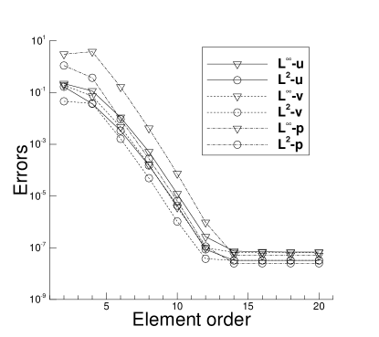
In this subsection we demonstrate the spatial and temporal convergence rates of the algorithm from Section 2 using a manufactured analytical solution to the Navier-Stokes equations. Consider the computational domain $\overline{ABCD}$ depicted in Figure 1(a), $0\leqslant x\leqslant 2$ and $-1\leqslant y\leqslant 1$, which is discretized by two equal-sized quadrilateral elements $\overline{ABFE}$ and $\overline{EFCD}$. Consider the following analytic solution to the equations (1a)–(1b),

$$\left\{\begin{split}&u=2\cos(\pi y)\sin(\pi x)\sin t,\\ &v=-2\sin(\pi y)\cos(\pi x)\sin t,\\ &p=2\sin(\pi y)\sin(\pi x)\cos t,\end{split}\right.$$ (52)

where $(u,v)$ are the $x$ and $y$ components of the velocity $\mathbf{u}$. In equation (1a) the non-dimensional viscosity is set to $\nu=0.01$, and the external force $\mathbf{f}$ is chosen in such a way that this equation is satisfied by the expressions in (52). Dirichlet boundary condition (3) is imposed on the boundaries $\overline{AB}$, $\overline{BC}$ and $\overline{AE}$, where the boundary velocity $\mathbf{w}(\mathbf{x},t)$ is chosen according to the analytic expressions from (52). The open boundary condition (5), with $\mathbf{H}(\mathbf{n},\mathbf{u})$ given by (6), is imposed on the boundaries $\overline{CD}$ and $\overline{DE}$, in which the parameters are set to $D_{0}=1$, $\delta=0.05$ and $U_{0}=1$, and the external boundary pressure force is set to $p_{0}=1$ on $\overline{CD}$ and $p_{0}=10$ on $\overline{DE}$. The source term $\mathbf{f}_{b}$ in (5) is chosen such that the analytic expressions from (52) satisfy the equation (5) on these boundaries. The initial velocity $\mathbf{u}_{in}$ is chosen based on the analytic expressions from (52) by setting $t=0$.

The method from Section 2 is employed to integrate the incompressible Navier-Stokes equations in time from $t=0$ to $t=t_{f}$ ($t_{f}$ to be specified below), in which we have employed a constant value $C_{0}=1$ in equation (10). We then compare the numerical solution at $t=t_{f}$ against the analytic solution of (52), and compute the error in various norms. The element order and the time step size $\Delta t$ are varied systematically to test the spatial and temporal convergence behavior of the method.

Figure 1(b) illustrates the behavior of the method for spatial convergence tests. Here we employ a fixed $t_{f}=0.1$ and $\Delta t=0.001$, and vary the element order between $2$ and $20$ in the tests. This figure shows the errors of the numerical solution at $t=t_{f}$ in $L^{\infty}$ and $L^{2}$ norms as a function of the element order. The result clearly exhibits an exponential convergence rate for element orders below $12$, and an error saturation for element orders above $12$, which is due to the dominance of the temporal truncation error at large element orders.

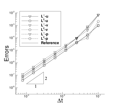
Figure 1(c) illustrates the temporal convergence behavior of the presented method. Here we have employed a fixed element order $16$ and $t_{f}=0.2$, and varied the time step size systematically between $\Delta t=0.1$ and $\Delta t=7.8125e-4$ in the tests. This figure shows the $L^{\infty}$ and $L^{2}$ errors of the numerical solution at $t=t_{f}$ as a function of $\Delta t$ for different flow variables. It is evident that the method exhibits a second-order convergence rate in time.

3.2 Flow in a Bifurcation Channel

Figure 2: Bifurcation channel: flow domain and the mesh of 2288 quadrilateral elements.

In this subsection we test our method using the bifurcation channel problem, which has been considered by a number of previous works (see e.g. PouxGA2011 ; DongKC2014 , among others)

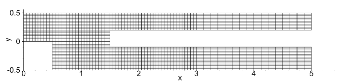
Specifically, we consider an incompressible flow contained in a bifurcation channel depicted in Figure 2. There are three openings in the channel: one on the left side ($x=0$), and two on the right ($x=5$). All the rest of the boundaries are walls. The flow enters the channel through the left opening, with a velocity profile assumed to be parabolic with a unit center-line velocity. External pressure heads are imposed on the two openings on the right sides, with $p_{01}$ on the upper right opening and $p_{02}$ on the lower right one. The values for $p_{01}$ and $p_{02}$ will be specified later.

We discretize the domain using a mesh of $2288$ quadrilateral elements as shown in Figure 2, with the element order varied in a range of values to be specified below. The method from Section 2 is employed to simulate the flow (with no external body force, i.e. $\mathbf{f}=0$ in (1a)). On the left boundary ($x=0$) the Dirichlet condition (3) is imposed, with the boundary velocity given according to the parabolic profile specified above. On the wall boundaries the no-clip condition (i.e. the Dirichlet condition (3) with $\mathbf{w}=0$) is imposed. On the right boundaries ($x=5$), the open boundary condition (5) is imposed, with $\mathbf{f}_{b}=0$ and $\mathbf{H}(\mathbf{n},\mathbf{u})$ given by (6) and with $p_{0}=p_{01}$ for the upper right boundary and $p_{0}=p_{02}$ for the lower right boundary.

Note that we have used the channel centerline velocity on the left boundary as the velocity scale ($U_{0}=1$), and the channel height in the mid-section ($0.5<x<1.5$) as the length scale. All the other parameters and variables are normalized accordingly. We focus on the Reynolds number $Re=800$ for this problem, chosen in accordance with DongKC2014 , and the flow is at a steady state. The other simulation parameters are set to $D_{0}=\frac{1}{U_{0}}=1$ and $\delta=0.05$. The element order, the time step size $\Delta t$, $C_{0}$, $p_{01}$ and $p_{02}$ are varied to study their effects on the flow characteristics.

Figure 3: Bifurcation channel: flow patterns visualized by streamlines.

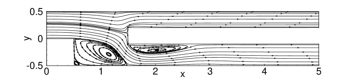
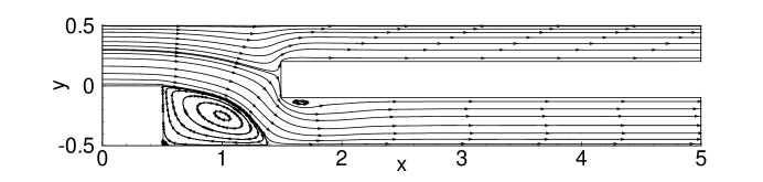
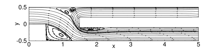
We first concentrate on the cases with zero external pressure heads at the two open boundaries on the right, namely, $p_{01}=p_{02}=0$. Figure 3 shows a visualization of the steady-state velocity patterns using streamlines, which are obtained with an element order $8$, time step size $\Delta t=0.001$ and $C_{0}=1$ in the simulations. In this case, the flow enters the domain through the left boundary and discharges from the domain through the two open boundaries on the right. Several re-circulation zones (bubbles) are visible from the flow pattern. The most prominent are those behind the inlet step and the one on the top wall of the lower bifurcation of the channel.

Element order	$f_{x}$	$f_{y}$	$L_{1}$	$L_{2}$
3	0.203	2.02e-3	0.970	1.24
4	0.196	-8.50e-5	0.975	1.23
5	0.193	-2.30e-4	0.980	1.23
6	0.192	-6.0e-6	0.980	1.22
7	0.191	1.25e-4	0.980	1.22
8	0.191	1.71e-4	0.980	1.22
9	0.191	1.86e-4	0.980	1.22
10	0.191	1.92e-4	0.980	1.22

Table 1: Resolution tests of the bifurcation channel problem. $f_{x}$ and $f_{y}$ are the $x$ and $y$ components of the total force on the channel walls. $L_{1}$ is the length on the bottom wall of the recirculation zone behind the inlet step. $L_{2}$ is the length of the recirculation zone on the top wall of the lower bifurcation.

We have varied the element order systematically in the simulations to make sure that the numerical results have converged with respect to the mesh resolution. Table 1 provides the $x$ and $y$ components of the total force ($f_{x}$ and $f_{y}$) exerting on the channel walls, as well as the sizes of the recirculation zones behind the inlet step ($L_{1}$) and on the top wall of the lower bifurcation ($L_{2}$), corresponding to different element orders. These results are obtained using a time step size $\Delta t=0.001$, and $C_{0}=1$ in equation (10). The mesh independence of the simulation results is evident for element orders beyond $6$.

(a) (b) (c) (d)

Figure 4: Bifurcation channel: Comparison of streamwise velocity profiles at several downstream locations, $x=0.25$ (a), $1.0$ (b), $2.0$ (c) and $4.0$ (d), computed using various element orders.

(a) (b) (c) (d)

Figure 5: Bifurcation channel: Comparison of vertical velocity profiles at several downstream locations, $x=0.25$ (a), $1.0$ (b), $2.0$ (c) and $4.0$ (d), computed using various element orders.

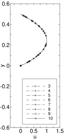
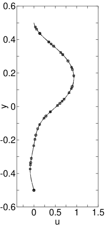
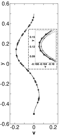
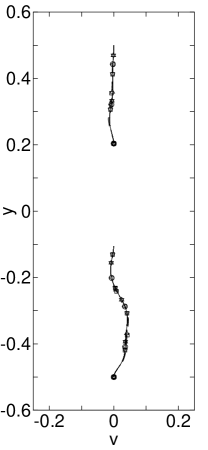
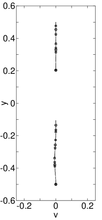
Figure 4 compares profiles of the streamwise velocity ($u$) along the $y$ direction at several downstream locations ($x=0.25$, $1.0$, $2.0$ and $4.0$), obtained with the range of element orders. Figure 5 is a corresponding comparison of the vertical velocity profiles at the same locations obtained with different element orders. Some magnified views of sections of the velocity profiles are provided in the insets of Figures 4(c) and 5(b). These results are computed with $\Delta t=0.001$ and $C_{0}=1$ in the simulations. It can be observed that the velocity profiles corresponding to element orders $6$ and beyond essentially overlap with one another, further attesting to the convergence of simulation results.

$\Delta t$	$\bar{f}_{x}$	$f^{\prime}_{x}$	$\bar{f}_{y}$	$f^{\prime}_{y}$
1e-4	0.192	0	1.16e-4	0
5e-4	0.191	0	1.54e-4	0
0.001	0.191	0	1.71e-4	0
0.005	0.144	1.23e-2	-6.57e-5	3.83e-3
0.01	0.139	9.88e-3	-3.13e-5	2.21e-3
0.05	0.126	3.99e-3	-6.46e-5	4.72e-4
0.1	0.123	1.94e-4	-6.01e-5	7.06e-4
0.5	0.119	1.97e-5	-1.03e-4	1.19e-4

Table 2: Bifurcation channel: forces on the channel walls obtained with a range of time step sizes $\Delta t$.

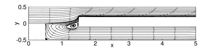
Thanks to the unconditional energy stability property (Theorem 2.1), stable computation results can be obtained using the current method even with large (or fairly large) time step sizes. This point is demonstrated by Table 2, in which we list the $x$ and $y$ forces on the wall ($f_{x}$ and $f_{y}$) obtained from the simulations using time step sizes ranging from $\Delta t=10^{-4}$ to $\Delta t=0.5$. These results correspond to an element order $8$ and $C_{0}=1$ in the simulations. We observe that when $\Delta t$ increases beyond a certain value ($5e-3$), the computed forces are no longer constant, but exhibit a fluctuation in their histories, although these fluctuations are minuscule. For such cases, $f_{x}$ and $f_{y}$ shown in Table 2 are the time-averaged forces, and $f_{x}^{\prime}$ and $f^{\prime}_{y}$ are the root-mean-square (rms) values. The stability of our method with large $\Delta t$ is evident. On the other hand, a deterioration in accuracy of the simulation result is visible when $\Delta t$ becomes large (or fairly large). Figure 6 shows a visualization of the flow pattern obtained with a larger time step size $\Delta t=0.01$. This figure can be compared with Figure 3, which corresponds to $\Delta t=0.001$. While the overall flow pattern in Figure 6 seems reasonable, the recirculation zone on the top wall of the lower bifurcation is markedly different in size compared with that of Figure 3.

Figure 6: Bifurcation channel: flow pattern visualized by streamlines obtained with a larger time step size $\Delta t=0.01$.

The above simulation results are obtained with the parameter values $D_{0}=1$ and $C_{0}=1$ in the computations. The parameters $D_{0}$ and $C_{0}$ have also been varied systematically ($D_{0}$ ranging from $0.1$ to $2.0$; $C_{0}$ ranging from $10^{-3}$ to $10^{6}$), and we observe no apparent effects of the variation of these parameters on the simulation results (e.g. in terms of the forces on the walls).

(a) (b) (c) (d)

Figure 7: Bifurcation channel: flow patterns visualized by streamlines corresponding to several external pressure heads imposed on the upper right boundary: (a) $p_{01}=-1.5$, (b) $p_{01}=-0.75$, (c) $p_{01}=0.75$, and (d) $p_{01}=1.5$. zero pressure head is imposed on the lower right boundary ($p_{02}=0$).

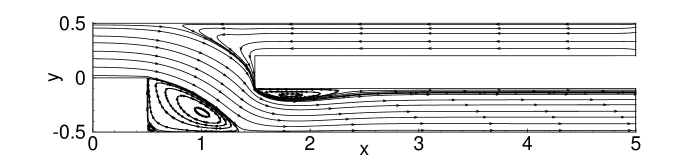
The incorporation of $p_{0}(\mathbf{x},t)$ in the open boundary condition (5) allows one to impose different pressure heads ($p_{01}$ and $p_{02}$) on the open boundaries of the bifurcation channel. Depending on the relative values of $p_{01}$ and $p_{02}$, the flow pattern in the domain can be modified dramatically. Figure 7 shows a comparison of the flow patterns visualized by streamlines corresponding to several $p_{01}$ values (ranging from $-1.5$ to $1.5$) at the upper right opening, while zero pressure head is imposed on the lower right one ($p_{02}=0$). These patterns can be compared with that of Figure 3, which corresponds to $p_{01}=p_{02}=0$. These results are obtained with an element order $8$, $\Delta t=0.001$, $D_{0}=1$ and $C_{0}=1$ in the simulations. When $p_{01}$ is sufficiently low compared with $p_{02}$, e.g. with $p_{01}=-1.5$ and $p_{02}=0$ (Figure 7(a)), the flow direction in the lower bifurcation can be reversed. In this case the lower right boundary effectively becomes an inlet, through which the flow is sucked into the domain. On the other hand, when $p_{01}$ is sufficiently high compared with $p_{02}$, e.g. with $p_{01}=1.5$ and $p_{02}=0$ (Figure 7(d)), a flow reversal occurs in the upper bifurcation. In this case, the upper right boundary becomes an effective inlet, and the flow is pushed into the domain through that boundary due to the high pressure head there.

$p_{01}$	$p_{02}$	$f_{x}$	$f_{y}$
-1.5	0	0.236	-1.65e-4
-0.75	0	0.239	-1.64e-4
0	0	0.191	1.71e-4
0.75	0	0.0230	5.30e-5
1.5	0	-0.163	-3.40e-4

Table 3: Forces on channel walls corresponding to different external pressure values on the upper outlet boundary.

3.3 Flow past a Circular Cylinder

Figure 8: Cylinder flow: flow configuration and a mesh of 1228 quadrilateral elements.

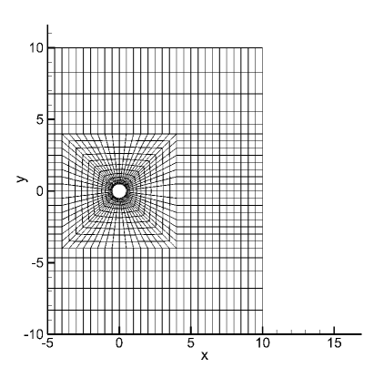
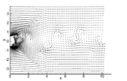
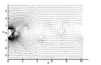
In this subsection we use a canonical problem, the flow past a circular cylinder, to test the performance of the method developed herein. Consider the flow domain depicted in Figure 8. The center of the cylinder coincides with the origin of the coordinate system. Let $d$ denote the cylinder diameter. On the left boundary ($x=-5d$), a uniform inflow with a velocity $U_{0}=1$ enters the domain in the horizontal direction. The flow exits the domain through the right boundary ($x=10d$), which is open. The top and bottom domain boundaries ($y=\pm 10d$) are assumed to be periodic. We choose $U_{0}$ and $d$ as the characteristic velocity and length scales, respectively, and all the parameters and variables are normalized accordingly. We would like to study the long-time behavior of this flow using the method developed here. As the Reynolds number becomes moderately large (around $Re=2000$ and beyond), vortices shed behind the cylinder can persist in the entire wake region and pass through the right open boundary, which can cause a severe issue to numerical simulations due to the backflow instability Dong2015clesobc ; DongS2015 ; NiYD2019 ; DongKC2014 .

We discretize the domain using a mesh of $1228$ quadrilateral spectral elements, as shown in Figure 8, and the element order is varied in the simulations. The method from Section 2 is employed to solve the incompressible Navier-Stokes equations, with $\mathbf{f}=0$ being set in (1a). Dirichlet boundary condition (3) is imposed on the left domain boundary, with the boundary velocity chosen based on the uniform inflow condition. No slip condition is imposed on the cylinder surface. Periodic conditions are imposed on the top/bottom boundaries for all flow variables. The open boundary condition (5), with $\mathbf{f}_{b}=0$, $D_{0}=\frac{1}{U_{0}}=1$, $p_{0}=0$, and $\delta=0.01$ in equation (6), is imposed on the right boundary. We employ a fixed $C_{0}=1$ in equation (10) in the simulations of this problem. The element order and the time step size $\Delta t$ have been varied systematically to investigate their effects on the simulation results. The flow at several Reynolds numbers ranging from $Re=30$ to $Re=10000$ has been simulated.

(a) (b)

Figure 9: Cylinder flow: instantaneous velocity distributions at Reynolds numbers (a) $Re=2000$, and (b) $Re=10000$.

(a) (b)

(c) (d)

Figure 10: Cylinder flow: time histories of the drag (plots (a) and (c)) and lift (plots (b) and (d)). Plots (a) and (b) are for $Re=100$, and plots (c) and (d) are for $Re=2000$.

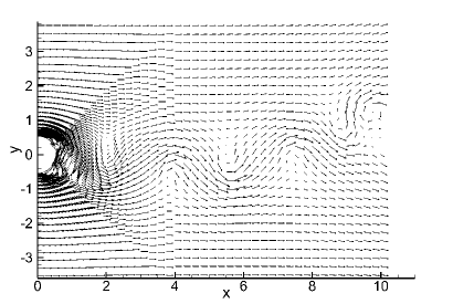
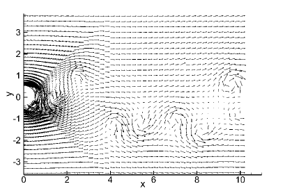
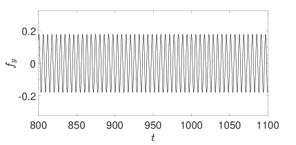
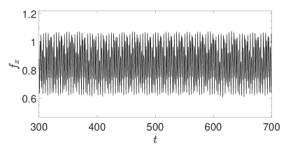
The cylinder flow is at a steady state for low enough Reynolds numbers (for $Re\lesssim 47$), and it becomes unsteady with vortex shedding behind the cylinder as the Reynolds number increases. We refer the reader to the review article Williamson1996 for a discussion of different flow regimes in the cylinder wake. Figure 9 shows instantaneous velocity field distributions at Reynolds numbers $Re=2000$ and $Re=10000$ obtained from current two-dimensional simulations. A train of irregular vortices can be observed behind the cylinder, which persist in the entire wake region at these Reynolds numbers with the current domain. In particular, vortices and backflows can be clearly observed at the outflow/open boundary, and they pose no problem to the current method. This is thanks to the energy-stable open boundary condition (5), which can effectively overcome the backflow instability issue (see Dong2015clesobc for details). Figure 10 shows a window of time histories of the drag and lift on the cylinder from current simulations for Reynolds numbers $Re=100$ and $Re=2000$, respectively. These forces fluctuate about some constant mean level, and their overall characteristics stay the same over time. These results demonstrate the long-term stability of our simulations, and show that the flow has reached a statistically stationary state.

Reynolds number	Method	Element order	mean drag	rms drag	mean lift	rms lift
30	Current	4	0.968	0	0	0
		5	0.968	0	0	0
		6	0.968	0	0	0
		7	0.968	0	0	0
		8	0.968	0	0	0
		9	0.968	0	0	0
		10	0.968	0	0	0
	Dong (2015)	–	0.968	0	0	0
	Dong & Shen (2015)	–	0.968	0	0	0
100	Current	4	0.729	3.79e-3	1.61e-4	0.127
		5	0.730	3.82e-3	9.16e-5	0.127
		6	0.729	3.81e-3	1.40e-4	0.127
		7	0.729	3.81e-3	-2.80e-5	0.127
		8	0.729	3.81e-3	2.15e-4	0.127
		9	0.729	3.81e-3	-6.50e-5	0.127
	Dong (2015)	–	0.729	–	–	0.127
	Dong & Shen (2015)	–	0.729	–	–	0.127
2000	Current	4	0.724	0.0996	1.46e-3	0.537
		5	0.863	0.117	3.53e-4	0.642
		6	0.893	0.125	-2.45e-5	0.699
		7	0.865	0.123	-4.66e-4	0.671
		8	0.853	0.123	-5.79e-4	0.657
		9	0.848	0.122	2.33e-3	0.653
	Dong (2015)	–	0.853	–	–	0.657

Table 4: Spatial resolution test for cylinder flow: mean and rms drag and lift forces on the cylinder computed using various element orders for several Reynolds numbers. The data from Dong (2015) Dong2015clesobc and Dong & Shen (2015) DongS2015 are included for comparison.

Based on the force history data, we can obtain the statistical quantities such as the time-averaged mean and root-mean-square (rms) forces. In current simulations we have varied the element order systematically between $4$ and $10$ to study its effect on the numerical result. In Table 4 we list the mean and rms drag and lift forces for several Reynolds numbers ($Re=30$, $100$ and $2000$) corresponding to different element orders. At $Re=30$ the flow is at a steady state, and so the values in the table are the steady-state forces and no time-averaging is performed for this Reynolds number. In these simulations the time step sizes are $\Delta t=1e-3$ for $Re=30$ and $100$, and $\Delta t=5e-4$ for $Re=2000$. For comparison, the forces obtained from Dong2015clesobc ; DongS2015 for these Reynolds numbers have also been included in this table. For the lower Reynolds numbers ($Re=30$ and $100$) the computed forces are basically the same using all these element orders. For the higher Reynolds number ($Re=2000$) we can observe a larger discrepancy between the obtained forces corresponding to the element orders $4$ and $5$ and those corresponding to higher element orders. On the other hand, when the element order increases to $7$ and higher, the obtained forces are quite close to one another, exhibiting a sense of convergence. The converged values of the forces from current simulations are in good agreement with those of Dong2015clesobc and DongS2015 . In subsequent simulations an element order $8$ is employed for this problem.

Reynolds number	$\Delta t$	mean drag	rms drag	mean lift	rms lift
30	0.001	0.968	0	0	0
	0.005	0.968	0	0	0
	0.01	0.968	0	0	0
	0.05	0.782	0.128	-3.21e-5	6.80e-3
	0.1	0.589	0.0950	-4.94e-5	4.42e-4
100	0.001	0.729	3.81e-3	2.15e-4	0.127
	0.005	0.729	3.81e-3	-1.72e-7	0.127
	0.01	0.550	0.128	2.15e-4	0.0616
	0.05	0.333	0.0823	1.95e-4	9.70e-3
	0.1	0.238	0.0461	1.195e-4	4.53e-3
2000	2.5e-4	0.853	0.123	-5.79e-4	0.657
	5.0e-4	0.855	0.123	6.71e-4	0.658
	0.001	0.504	0.288	2.54e-3	0.440
	0.005	0.167	0.0896	3.90e-4	0.179
	0.01	0.0898	0.0578	-3.2e-4	0.0780
	0.05	0.0251	7.16e-3	-5.83e-3	2.08e-3
	0.1	0.0205	1.05e-3	1.06e-4	9.48e-4

Table 5: Cylinder flow: mean and rms drag and lift forces obtained with a range of time steps sizes $\Delta t$ for several Reynolds numbers.

Thanks to the unconditional energy stability property, stable simulation results can be obtained using our method irrespective of the time step size. We have varied $\Delta t$ systematically and performed simulations using these $\Delta t$ values for several Reynolds numbers. Table 5 lists the mean and rms forces on the cylinder computed using different $\Delta t$ values at three Reynolds numbers $Re=30$, $100$ and $2000$. The element order is fixed at $8$ in these tests. Long-time simulations have been performed with each $\Delta t$, and the statistical quantities shown in the table are computed based on the drag and lift histories from these simulations. These results attest to the stability of simulations using the current method, even with large (or fairly large) $\Delta t$ values. It can also be observed that the accuracy of the simulation results could deteriorate when $\Delta t$ becomes large. For example, at $Re=30$ it should physically be a steady flow. However, with larger time step sizes (e.g. $\Delta t=0.05$ and $0.1$) the obtained velocity fields actually become unsteady, and there is a notable difference between the computed mean and rms drag values when compared with those corresponding to smaller $\Delta t$. At higher Reynolds numbers, the computed values for the mean and rms drags and lifts with large $\Delta t$ appear smaller than those corresponding to small $\Delta t$. These tests suggest that, while the method is unconditionally energy stable and can produce stable results with various time step sizes ranging from small to large values, the result corresponding to a large $\Delta t$ should only serve as a reference solution and should not be blindly trusted. Convergence tests should be performed with respect to the simulation parameters (e.g. $\Delta t$ and spatial resolution) using the current method, as well as with any other numerical method for that matter.

(a) (b)

(c) (d)

(e) (f)

(g) (h)

Figure 11: Cylinder flow ($Re=5000$): temporal sequence of snapshots of velocity distributions: (a) $t=1208.9$, (b) $t=1209.5$, (c) $t=1210.1$, (d) $t=1210.7$, (e) $t=1211.3$, (f) $t=1211.9$, (g) $t=1212.5$, (h) $t=1213.1$. Velocity vectors are plotted on a sparser grid for clarity.

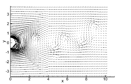
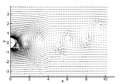
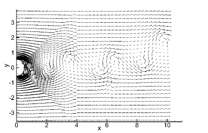
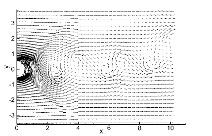
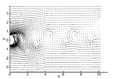
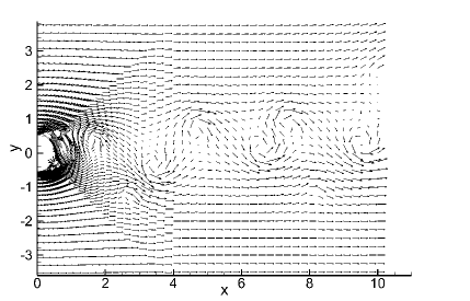
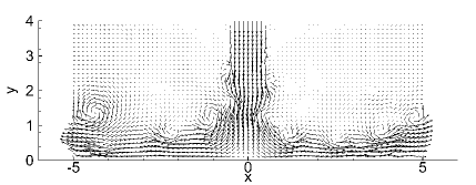
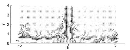
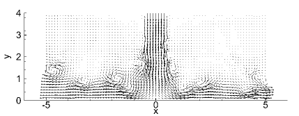
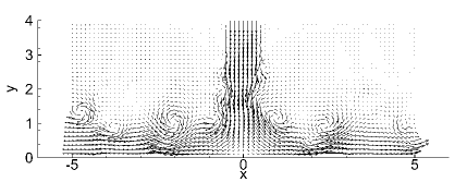
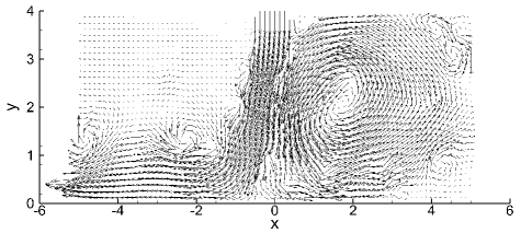
Finally, Figure 11 illustrates the dynamics of the cylinder flow with a temporal sequence of snapshots (with a time interval $0.6$ between consecutive frames) of the velocity distributions at $Re=5000$. Vortex shedding behind the cylinder generates a Karman vortex street in the wake. As the vortices exit the domain, backflows can be observed at the outflow/open boundary; see e.g. Figures 11(b)–(e) and (f)–(h). While some distortions to the vortices are evident, it is observed that the current method can allow the vortices to cross the outflow/open boundary in a fairly smooth and natural fashion.

3.4 Jet Impinging on a Wall

Figure 12: Impinging jet: flow configuration and boundary conditions.

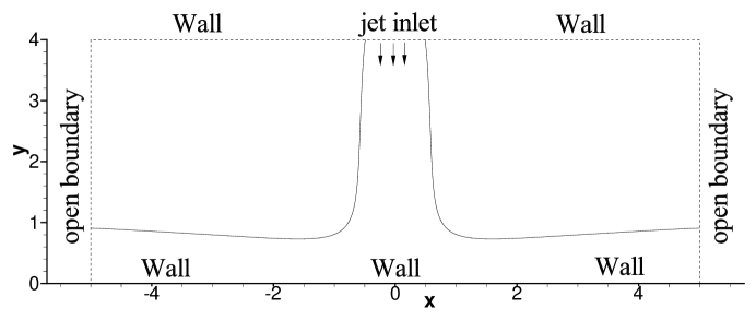
In the last numerical test we simulate a jet impinging on a wall using the current method. A sketch of the problem configuration is shown in Figure 12. We consider a rectangular domain, $-5\leqslant x/d\leqslant 5$ and $0\leqslant y/d\leqslant 4$, where $d=1$ denotes the diameter of the jet at the inlet. The top and bottom of the domain are solid walls. A jet stream is introduced into the domain through an opening in the middle of the top wall, with a diameter $d$. The jet velocity at the inlet is assumed to have the following distribution:

$$\left\{\begin{split}&u=0\\ &v=-U_{0}\left(\left[H(x,0)-H(x,R_{0})\right]\tanh\frac{1-x/R_{0}}{\sqrt{2}\epsilon}+\left[H(x,-R_{0})-H(x,0)\right]\tanh\frac{1+x/R_{0}}{\sqrt{2}\epsilon}\right)\end{split}\right.$$ (53)

where $U_{0}=1$ denotes the velocity scale, $R_{0}=d/2$ is the jet radius, and $\epsilon=d/40$. $H(x,a)$ is the Heaviside step function, taking a unit value if $x\geqslant a$ and vanishing otherwise. The left and right sides of the domain are open, and the fluids can freely leave or enter the domain through these boundaries. A pressure head is imposed on the open boundaries, with $p_{01}$ on the left boundary and $p_{02}$ on the right one. The jet stream enters the domain through the inlet and, depending on the relative levels for $p_{01}$ and $p_{02}$, may exit the domain through both sides or through only one side of the open boundary.

All the parameters and variables are normalized with the velocity scale $U_{0}$ and the length scale $d$. We discretize the domain using a mesh of $640$ equal-sized quadrilateral spectral elements, with $40$ elements along the horizontal direction and $16$ elements along the vertical direction. The method from Section 2 is employed to simulate the incompressible Navier-Stokes equations, with $\mathbf{f}=0$ in equation (1a). The Dirichlet condition (3) is imposed on the wall boundaries, with the boundary velocity set to $\mathbf{w}=0$, and also at the jet inlet, with the boundary velocity $\mathbf{w}$ set according to equation (53). The boundary condition (5) is imposed on the left and right open boundaries, with $\mathbf{f}_{b}=0$, $D_{0}=\frac{1}{U_{0}}=1$ and $\delta=0.01$. The external pressure force in (5) is set to $p_{0}=p_{01}$ on the left boundary and $p_{0}=p_{02}$ on the right boundary. The Reynolds number, the element order, the time step size $\Delta t$, and the external pressure heads $p_{01}$ and $p_{02}$ have been varied to study their effects on the flow characteristics. We employ a constant $C_{0}=1$ in simulations for this problem. Long-time simulations have been performed such that the flow has reached a statistically stationary state. Therefore the initial velocity has no effect on the results reported below.

(a) (b) (c)

Figure 13: Impinging jet: velocity distributions at Reynolds numbers (a) $Re=300$, (b) $Re=2000$, and (c) $Re=5000$. Velocity vectors are plotted on a set of sparser grid points for clarity.

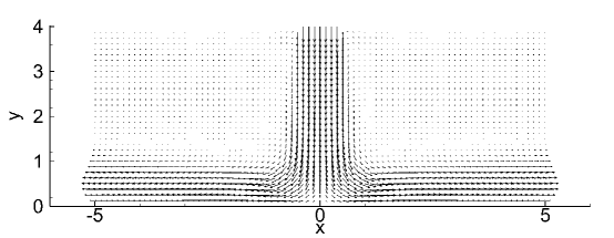
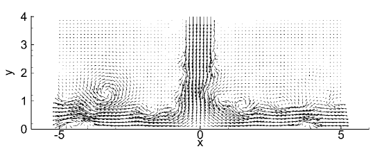
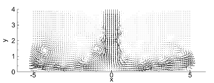
Let us first focus on the cases with zero external pressure heads on the left and right open boundaries ($p_{01}=p_{02}=0$). Figure 13 provides an overview of the flow characteristics of this problem for several Reynolds numbers. At $Re=300$ it is a steady flow (Figure 13(a)). After impinging on the bottom wall, the vertical jet splits into two horizontal streams near the wall, which flow out of the domain through the left and right open boundaries. It is noted that strong flows mostly occupy the regions near the bottom wall or near the domain centerline ($x/d=0$), while in the rest of the domain the flow is quite weak. With the increase of Reynolds number, the flow becomes unsteady. A train of vortices are observed to form along the profile of the vertical jet or the near-wall horizontal streams (Figures 13(b)-(c)), which travel along with the jet and leave the domain through the open boundaries.

(a) (b)

Figure 14: Impinging jet (Re=2000): time histories of the x-component (a) and y-component (b) of the force on the walls.

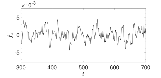
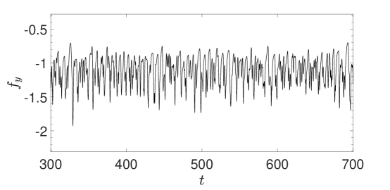
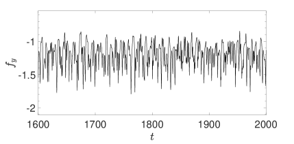
Figure 14 shows a window of the time histories of the total force ($x$ and $y$ components) exerting on the domain walls at $Re=2000$, which corresponds to the case shown in Figure 13(b). These results are obtained with an element order $6$ and a time step size $\Delta t=0.001$. One can note that the forces are highly unsteady and fluctuational. The horizontal force is very weak and essentially negligible compared with the vertical force, because of symmetry and the zero pressure heads imposed on the left and right boundaries. The long time histories indicate that the flow has indeed reached a statistically stationary state and that the simulation is long-time stable.

$Re$	Element order	$\overline{f}_{x}$	$f^{\prime}_{x}$	$\overline{f}_{y}$	$f^{\prime}_{y}$
300	4	0	0	-0.965	0
	5	0	0	-0.975	0
	6	0	0	-0.984	0
	7	0	0	-0.986	0
	8	0	0	-0.987	0
2000	4	3.44e-5	1.63e-3	-1.131	0.201
	5	-8.23e-5	1.69e-3	-1.089	0.191
	6	-1.71e-4	1.76e-3	-1.100	0.198
	7	-1.20e-5	1.66e-3	-1.103	0.201
	8	-9.17e-5	1.61e-3	-1.106	0.205
5000	4	3.60e-5	9.82e-4	-1.117	0.195
	5	4.94e-6	1.04e-3	-1.092	0.210
	6	-1.98e-5	1.09e-3	-1.078	0.223
	7	-2.24e-6	1.09e-3	-1.068	0.230
	8	-4.13e-5	1.03e-3	-1.076	0.235

Table 6: Impinging jet: Effect of element order on the computed forces on the walls.

$Re$	$\Delta t$	$\overline{f}_{x}$	$f^{\prime}_{x}$	$\overline{f}_{y}$	$f^{\prime}_{y}$
300	0.0005	0	0	-0.983	0
	0.001	0	0	-0.984	0
	0.005	0	0	-0.986	0
	0.01	0	0	-0.986	0
	0.05	-2.37e-3	7.61e-7	-0.270	3.82e-3
	0.1	-2.69e-4	8.74e-5	-0.183	1.17e-3
	0.5	7.65e-5	4.27e-6	-0.098	5.09e-4
2000	0.0005	-8.93e-5	1.73e-3	-1.095	0.197
	0.001	-1.71e-4	1.76e-3	-1.100	0.198
	0.005	-2.58e-5	1.77e-3	-1.069	0.244
	0.01	-6.06e-5	3.54e-3	-0.576	0.391
	0.05	5.93e-5	2.02e-3	-0.114	0.0624
	0.1	-9.34e-4	1.20e-6	-0.0609	0.0144
5000	0.0005	1.84e-5	1.14e-3	-1.087	0.223
	0.001	-1.98e-5	1.09e-3	-1.078	0.223
	0.005	-3.38e-5	4.09e-3	-0.742	0.578
	0.01	-2.05e-4	3.97e-3	-0.384	0.459
	0.05	4.05e-5	1.47e-3	-0.0829	0.0924
	0.1	-2.25e-5	9.16e-4	-0.0562	0.0406

Table 7: Impinging jet: Effect of $\Delta t$ on the computed forces on the walls.

We can obtain the statistical quantities such as the mean and rms forces the jet exerts on the domain walls based on the force signals like those shown in Figure 14. To investigate the mesh resolution effect, we have performed simulations using a range of element orders. In Table 6 we list the time-averaged mean and rms forces on the wall computed using different element orders at three Reynolds numbers $Re=300$, $2000$ and $5000$. The flow at $Re=300$ is steady, and so shown in the table are the steady-state forces and no time-averaging is performed. It can be observed that with element orders $6$ and larger there is little difference in the obtained mean and rms force values, demonstrating a convergence with respect to the mesh resolution. The majority of subsequent simulations for this problem are performed with an element order $6$.

The current method produces stable simulation results for the impinging jet problem, with various time step sizes ranging from small to large values. This is demonstrated by Table 7, in which the mean and rms forces obtained with a range of $\Delta t$ values have been shown for the Reynolds numbers $Re=300$, $2000$ and $5000$. The deterioration in accuracy of the obtained results when $\Delta t$ becomes large can also be observed here, similar to the observation from Section 3.3. Differences between the mean/rms forces corresponding to large (or fairly large) $\Delta t$ values and those corresponding to small $\Delta t$ are evident, indicating a deterioration or loss of accuracy when $\Delta t$ becomes too large.

(a) (b)

(c) (d)

(e) (f)

(g) (h)

Figure 15: Impinging jet (Re=5000): temporal sequence of snapshots of the velocity fields at instants (a) $t=1569$, (b) $t=1570.2$, (c) $t=1571.4$, (d) $t=1572.6$, (e) $t=1573.8$, (f) $t=1575$, (g) $t=1576.2$, (h) $t=1577.4$. Velocity vectors are shown on a set of sparser grid points for clarity.

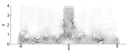
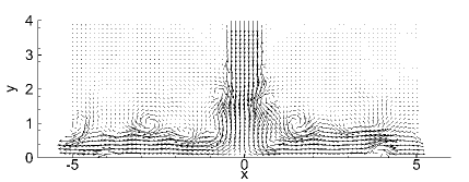
Figure 15 illustrates the dynamical features of the impinging jet problem with a temporal sequence of snapshots of the velocity fields at $Re=5000$. These results correspond to zero external pressure heads ($p_{01}=p_{02}=0$) on the open boundaries. They are computed with an element order $7$, a time step size $\Delta t=0.001$, and the open boundary condition (5) with $\mathbf{H}(\mathbf{n},\mathbf{u})$ given by (8) having parameter values $(\theta,\alpha_{1},\alpha_{2})=(0,1,1)$. A stable region immediately downstream of the jet inlet can be observed. This region shrinks with increasing Reynolds number. At $Re=5000$ this stable region appears to be shorter than a jet diameter (Figure 15). Downstream of this stable region, the vertical jet experiences the Kelvin-Helmholtz instability and the shear layers roll up to form vortices along the profile of the jet stream (Figures 15(b)-(d)). These vortices persist along the outgoing horizontal streams, forming a train of vortices in the domain (Figures 15(c)-(h)). These vortices are ultimately discharged from the domain through the left and the right open boundaries (see Figures 15(d)-(h)). The presence of backflows and the passage of strong vortices on the open boundaries make the impinging jet problem very challenging to simulate. The energy-stable open boundary condition (5), and those developed in e.g. DongS2015 ; Dong2015clesobc ; DongKC2014 ; NiYD2019 , are critical to dealing with such open boundaries and the successful simulation of this problem.

(a) (b)

Figure 16: Impinging jet (Re=300): effect of external pressure heads on the flow field. External pressure force on the right boundary is fixed at $p_{02}=0$, and on the left boundary it corresponds to (a) $p_{01}=0.2$ and (b) $p_{01}=0.4$.

(a) (b) (c)

Figure 17: Impinging jet (Re=5000): effect of external pressure heads on the flow field. External pressure force on the left boundary is fixed at $p_{01}=0$, and on the right boundary it corresponds to (a) $p_{02}=0.2$, (b) $p_{02}=0.3$, and (c) $p_{02}=0.4$.

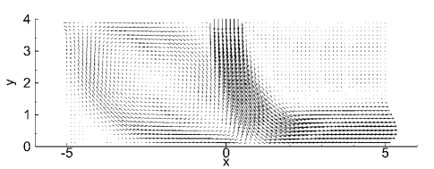
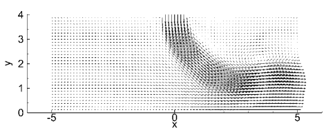
Let us next look into the effect of non-zero external pressure heads ($p_{01}$ and $p_{02}$) on the impinging jet problem. Depending on the relative values of $p_{01}$ and $p_{02}$, the flow loses symmetry and the pressure difference can induce a horizontal flow, which if sufficiently strong will bend the jet toward one side. Figures 16 and 17 demonstrates these scenarios with Reynolds numbers $Re=300$ and $Re=5000$, respectively. In Figure 16, on the right open boundary a zero pressure head ($p_{02}=0$) is imposed, and the external pressure on the left open boundary ($p_{01}$) is varied. The two plots in Figure 16 correspond to $p_{01}=0.2$ and $p_{01}=0.4$, respectively. In Figure 17, on the left open boundary a zero pressure head ($p_{01}=0$) is imposed, while the external pressure head on the right open boundary ($p_{02}$) is varied. The plots in Figure 17 correspond to $p_{02}=0.2$, $0.3$ and $0.4$ in the simulations, respectively. We indeed observe that the jet can be bent toward the right (Figure 16) or the left (Figure 17) because of the external pressure difference in the horizontal direction. When this pressure difference is not strong enough to overcome the upcoming horizontal jet stream, the horizontal stream may be deflected to form a large vortex on one side of the domain (see Figures 16(a) and 17(a)). With a strong enough pressure difference, a horizontal flow can be established in the domain and the jet is pushed toward one side (see Figure 16(b) and Figures 17(b)-(c)).

(a) (b)

(c) (d)

Figure 18: Impinging jet (Re=5000): time histories of the x-component (plots (a) and (c)) and y-component (plots (b) and (d)) of the force on the wall. Plots of (a) and (b) correspond to zero external pressure force $p_{01}=p_{02}=0$, and those in (c) and (d) correspond to external pressure forces $p_{01}=0$ and $p_{02}=0.3$.

Non-zero external pressure heads can also cause the force exerting on the wall to differ markedly when compared with the case of zero external pressure heads. Figure 18 shows time histories of the two components of the total force on the walls at $Re=5000$ corresponding to a zero pressure head ($p_{01}=p_{02}=0$, plots (a) and (b)) and a non-zero pressure head ($p_{01}=0$ and $p_{02}=0.3$, (c) and (d)). We observe that the external pressure difference induces a mean horizontal force on the walls, while with zero external pressure heads the mean horizontal force is essentially zero.

4 Concluding Remarks

In the current work we have developed an unconditionally energy-stable scheme for simulating incompressible flows on domains with outflow/open boundaries. This scheme combines the generalized Positive Auxiliary Variable (gPAV) approach and a rotational velocity-correction type strategy. The incompressible Navier-Stokes equations, the dynamic equation for the auxiliary variable, and the energy-stable open boundary conditions have been reformulated based on the gPAV idea. The discrete unconditional energy stability of the proposed scheme has been proven. Within each time step, the scheme requires the computation of two velocity fields and two pressure fields in a fully de-coupled fashion, by solving several individual linear equations involving constant and time-independent coefficient matrices. The auxiliary variable, being a scalar number rather than a field function, is given by a well-defined explicit formula, and its computed values are guaranteed to be positive. It should be noted that no nonlinear solver is involved in the current method for either the field functions or the auxiliary variable, and the linear algebraic systems to be solved involve only constant coefficient matrices that can be pre-computed. Therefore, the current scheme is computationally very attractive and competitive.

Extensive numerical experiments have been provided with a number of flow problems involving outflow/open boundaries. In particular the flow regimes with backflow instability have been simulated, in which strong vortices or backflows can occur at the outflow/open boundaries. These numerical tests demonstrate the stability of the proposed scheme with various time step sizes ranging from small to large values. At the same time these tests also show a deterioration in accuracy of the simulation results when the time step size becomes too large. These observations suggest that the simulation result using a large time step size should only serve as a reference solution, which cannot be fully trusted unless appropriate convergence tests with respect to the simulation parameters (such as the time step size) are performed. The use of an unconditionally energy-stable scheme such as the one presented herein (and any other numerical scheme for that matter) is no substitute for the convergence tests in actual production simulations.

It is worth comparing the scheme developed here with that from the recent work LinYD2019 , as both schemes employ an auxiliary variable in the algorithmic construction. In Remark 2.3 we have commented on this matter in some detail. Here we would like to emphasize two points:

• While an auxiliary variable is used in both schemes, the reformulated system and its numerical treatment are completely different in the current scheme compared with that of LinYD2019 . In the current method it is guaranteed that the solution for the auxiliary variable exists, that it is given by an explicit formula, and that its computed value is positive. In contrast, in LinYD2019 the auxiliary variable is obtained by solving a nonlinear algebraic equation. Consequently, the solution for the auxiliary variable cannot be guaranteed to exist in LinYD2019 . Even when it exists, the computed value is not guaranteed to be positive, even though this variable should physically be. Some nonlinear algebraic solver such as the Newton’s method is required in LinYD2019 . In the current method, on the other hand, no nonlinear solver is involved, for either the field functions or the auxiliary variable.

• In the algorithmic formulation of the current scheme, the pressure and the velocity are de-coupled (barring the auxiliary variable) in a way that mirrors a rotational velocity-correction strategy. The discrete unconditional energy stability has been proven with this de-coupled formulation. In contrast, in the algorithmic formulation of LinYD2019 the pressure and the velocity are fully coupled, and the discrete energy stability can only be proven in this fully coupled setting therein.

Another salient feature of the current scheme lies in the use of the function $g(\frac{R^{2}}{E})$ (defined in (13)), rather than $\frac{R^{2}}{E}$, when reformulating the incompressible Navier-Stokes equation (see equation (14)). This construction can improve the accuracy when small time step sizes are used in simulations. While $\frac{R^{2}}{E}$ should physically equal the unit value on the continuum level, its numerically-computed value is rarely exactly the unit value. Numerical experiments indicate that, with small time step sizes, the computed values for $\frac{R^{2}}{E}$ are very close to $1.0$, but typically slightly larger than $1.0$ by a minuscule amount (e.g. $10^{-6}$). This can introduce an error, while small, if $\frac{R^{2}}{E}$ itself is used when reformulating the Navier-Stokes equation in (14). The use of the function $g(\frac{R^{2}}{E})$ can get rid of this error and improve the accuracy of simulations with small time step sizes.

Regarding the computational cost, because the current method requires the solution of two copies of the flow field variables (velocity and pressure), the amount of operations per time step in the current method is approximately twice that with a typical semi-implicit scheme (see e.g. Dong2015clesobc ), which is only conditionally stable.

References

- [1] M.O. Abu-Al-Saud, A. Riaz, and H.A. Tchelepi. Multiscale level-set method for accurate modeling of immiscible two-phase flow with deposited thin films on solid surfaces. Journal of Computational Physics, 333:297–320, 2017.
- [2] Y. Bazilevs, J.R. Hohean, T.J.R. Hughes, R.D. Moser, and Y. Zhang. Patient-specific isogeometric fluid-structure interaction analysis of theracic aortic blood flow due to impantation of the jarvik 2000 left ventricular assist device. Comput. Methods Appl. Mech. Engrg., 198:3534–3550, 2009.
- [3] C. Bertoglio and A. Caiazzo. A tangential regularization method for backflow stabilization in hemodynamics. Journal of Computational Physics, 261:162–171, 2014.
- [4] C. Bertoglio and A. Caiazzo. A stokes-residual backflow stabilization method applied to physiological flows. Journal of Computational Physics, 313:260–278, 2016.
- [5] D.L. Brown, R. Cortez, and M.L. Minion. Accurate projection methods for the incompressible Navier-Stokes equations. J. Comput. Phys., 168:464–499, 2001.
- [6] C.-H. Bruneau and P. Fabrie. Effective downstream boundary conditions for incompressible Navier-Stokes equations. International Journal for Numerical Methods in Fluids, 19:693–705, 1994.
- [7] C.-H. Bruneau and P. Fabrie. New efficient boundary conditions for incompressible navier-stokes equations: a well-posedness result. Mathematical Modeling and Numerical Analysis, 30:815–840, 1996.
- [8] H. Chen, S. Sun, and T. Zhang. Energy stability analysis of some fully discrete numerical schemes for incompressible navier-stokes equations on staggered grids. Journal of Scientific Computing, 75:427–456, 2018.
- [9] L. Chen, J. Shen, and C.J. Xu. A unstructured nodal spectral-element method for the navier-stokes equations. Communications in Computational Physics, 12:315–336, 2012.
- [10] A.J. Chorin. Numerical solution of the Navier-Stokes equations. Math. Comput., 22:745–762, 1968.
- [11] S. Dong. Evidence for internal structures of spiral turbulence. Physical Review E, 80:067301, 2009.
- [12] S. Dong. An efficient algorithm for incompressible N-phase flows. Journal of Computational Physics, 276:691–728, 2014.
- [13] S. Dong. An outflow boundary condition and algorithm for incompressible two-phase flows with phase field approach. Journal of Computational Physics, 266:47–73, 2014.
- [14] S. Dong. A convective-like energy-stable open boundary condition for simulations of incompressible flows. Journal of Computational Physics, 302:300–328, 2015.
- [15] S. Dong. Wall-bounded multiphase flows of N immiscible incompressible fluids: consistency and contact-angle boundary condition. Journal of Computational Physics, 338:21–67, 2017.
- [16] S. Dong, G.E. Karniadakis, and C. Chryssostomidis. A robust and accurate outflow boundary condition for incompressible flow simulations on severely-truncated unbounded domains. Journal of Computational Physics, 261:83–105, 2014.
- [17] S. Dong, G.E. Karniadakis, A. Ekmekci, and D. Rockwell. A combined direct numerical simulation-particle image velocimetry study of the turbulent near wake. J. Fluid Mech., 569:185–207, 2006.
- [18] S. Dong and J. Shen. An unconditionally stable rotational velocity-correction scheme for incompressible flows. Journal of Computational Physics, 229:7013–7029, 2010.
- [19] S. Dong and J. Shen. A time-stepping scheme involving constant coefficient matrices for phase field simulations of two-phase incompressible flows with large density ratios. Journal of Computational Physics, 231:5788–5804, 2012.
- [20] S. Dong and J. Shen. A pressure correction scheme for generalized form of energy-stable open boundary conditions for incompressible flows. Journal of Computational Physics, 291:254–278, 2015.
- [21] S. Dong and X. Wang. A rotational pressure-correction scheme for incompressible two-phase flows with open boundaries. PLOS One, 11(5):e0154565, 2016.
- [22] N.S. Ghaisas, D.A. Shetty, and S.H. Frankel. Large eddy simulation of turbulent horizontal buoyant jets. Journal of Turbulence, 16:772–808, 2015.
- [23] V. Gravemeier, A. Comerford, L. Yoshihara, M. Ismail, and W.A. Wall. A novel formulation for Neumann inflow boundary conditions in biomechanics. International Journal for Numeical Methods in Biomedical Engineering, 28:560–573, 2012.
- [24] P.M. Gresho. Incompressible fluid dynamics: some fundamental formulation issues. Annual Review of Fluid Mechanics, 23:413–453, 1991.
- [25] J.L. Guermond, P. Minev, and J. Shen. Error analysis of pressure-correction schemes for the time-dependent stokes equations with open boundary conditions. SIAM J. Numer. Anal., 43:239–258, 2005.
- [26] J.L. Guermond, P. Minev, and J. Shen. An overview of projection methods for incompressible flows. Comput. Methods Appl. Mech. Engrg., 195:6011–6045, 2006.
- [27] J.L. Guermond and J. Shen. A new class of truly consistent splitting schemes for incompressible flows. J. Comput. Phys., 192:262–276, 2003.
- [28] B. Hyoungsu and G.E. Karniadakis. Subiteration leads to accuracy and stability enhancements of semi-implicit schemes for the navier-stokes equations. Journal of Computational Physics, 230:4384–4402, 2011.
- [29] M. Ismail, V. Gravemeier, A. Comerford, and W.A. Wall. A stable approach for coupling multidimensional cardiovascular and pulmonary networks based on a novel pressure-flow rate or pressure-only neumann boundary condition formulation. International Journal for Numerical Methods in Biomedical Engineering, 30:447–469, 2014.
- [30] N. Jiang, M. Mohebujjaman, L.G. Rebholz, and C. Trenchea. An optimally accurate discrete regularization for second order timestepping methods for navier-stokes equations. Comput. Methods Appl. Mech. Engrg., 310:388–405, 2016.
- [31] G.E. Karniadakis, M. Israeli, and S.A. Orszag. High-order splitting methods for the incompressible Navier-Stokes equations. J. Comput. Phys., 97:414–443, 1991.
- [32] G.E. Karniadakis and S.J. Sherwin. Spectral/hp element methods for computational fluid dynamics, 2nd edn. Oxford University Press, 2005.
- [33] J. Kim and P. Moin. Application of a fractional-step method to incompressible Navier-Stokes equations. J. Comput. Phys., 59:308–323, 1985.
- [34] A.G. Kravchenko and P. Moin. Numerical studies of flow over a circular cylinder at Re. Physics of Fluids, 12:403–417, 2000.
- [35] A. Labovsky, W.J. Layton, C.C. Manica, M. Neda, and L.G. Rebholz. The stabilized extrapolated trapezoidal finite-element method for the Navier-Stokes equations. Comput. Methods Appl. Mech. Engrg., 198:958–974, 2009.
- [36] M.S. Lee, A. Riaz, and V. Aute. Direct numerical simulation of incompressible multiphase flow with phase change. Journal of Computational Physics, 344:381–418, 2017.
- [37] L. Lin, Z. Yang, and S. Dong. Numerical approximation of incompressible Navier-Stokes equations based on an auxiliary energy variable. Journal of Computational Physics, 388:1–22, 2019.
- [38] J.-G. Liu, J. Liu, and R.L. Pego. Stability and convergence of efficient Navier-Stokes solvers via a commutator estimate. Comm. Pure Appl. Math., LX:1443–1487, 2007.
- [39] M.E. Moghadam, Y. Bazilevs, T.-Y. Hsia, I.E. Vignon-Clementel, and A.L. Marsden. A comparison of outlet boundary treatments for prevention of backflow divergence with relevance to blood flow simulations. Comput. Mech., 48:277–291, 2011.
- [40] N. Ni, Z. Yang, and S. Dong. Energy-stable boundary conditions based on a quadratic form: Applications to outflow/open-boundary problems in incompressible flows. Journal of Computational Physics, 391:179–215, 2019.
- [41] A. Porpora, P. Zunino, C. Vergara, and M. Piccinelli. Numerical treatment of boundary conditions to replace branches in hemodynamics. International Journal of Numerical Methods in Biomedical Engineering, 28:1165–1183, 2012.
- [42] A. Poux, S. Glockner, and M. Azaiez. Improvements on open and traction boundary conditions for navier-stokes time-splitting methods. Journal of Computational Physics, 230:4011–4027, 2011.
- [43] B. Sanderse. Energy-conserving runge-kutta methods for the incompressible navier-stokes equations. J. Comput. Phys., 233:100–131, 2013.
- [44] D. Serson, J.R. Meneghini, and S.J. Sherwin. Velocity-correction schemes for the incompressible navier-stokes equations in general coordinate systems. Journal of Computational Physics, 316:243–254, 2016.
- [45] J. Shen. On error estimate of projection methods for Navier-Stokes equations: first-order schemes. SIAM J. Numer. Anal., 29:57–77, 1992.
- [46] J. Shen, J. Xu, and J. Yang. The scalar auxiliary variable (sav) approach for gradient flows. Journal of Computational Physics, 353:407–416, 2018.
- [47] S.J. Sherwin and G.E. Karniadakis. A triangular spectral element method: applications to the incompressible navier-stokes equations. Comput. Meth. Appl. Mech. Engrg., 123:189–229, 1995.
- [48] J.C. Simo and F. Armero. Unconditional stability and long-term behavior of transient algorithms for the incompressible Navier-Stokes and Euler equations. Comput. Methods Appl. Mech. Engrg., 111:111–154, 1994.
- [49] R. Temam. Sur l’approximation de la solution des equations de Navier-Stokes par la methods des pas fractionnaires ii. Arch. Ration. Mech. Anal., 33:377–385, 1969.
- [50] S.S. Varghese, S.H. Frankel, and P.F. Fischer. Direct numerical simulation of stenotic flows. Part 1. steday flow. Journal of Fluid Mechanics, 582:253–280, 2007.
- [51] R.W.C.P. Verstappen and A.E.P. Veldman. Symmetry-preserving discretization of turbulent flow. Journal of Computational Physics, 187:343–368, 2003.
- [52] C.H.K. Williamson. Vortex dynamics in a cylinder wake. Annual Review of Fluid Dynamics, 28:477–539, 1996.
- [53] C.J. Xu and R. Pasquetti. On the efficiency of semi-implicit and semi-lagrangeian spectral methods for the calculation of incompressible flows. International Jurnal for Numerical Methods in Fluids, 35:319–340, 2001.
- [54] Z. Yang and S. Dong. A roadmap for discretely energy-stable schemes for dissipative systems based on a generalized auxiliary variable with guaranteed positivity. arXiv:1904.00141.
- [55] Z. Yang and S. Dong. An unconditionally energy-stable scheme based on an implicit auxiliary energy variable for incompressible two-phase flows with different densities involving only precomputable coefficient matrices. Journal of Computational Physics, 393:229–257, 2019.
- [56] Z. Yang, L. Lin, and S. Dong. A family of second-order energy-stable schemes for Cahn-Hilliard type equations. Journal of Computational Physics, 383:24–54, 2019.
- [57] X. Zheng and S. Dong. An eigen-based high-order expansion basis for structured spectral elements. Journal of Computational Physics, 230:8573–8602, 2011.