Nonequilibrium path-ensemble averages for symmetric protocols

Abstract

According to the nonequilibrium work relations, path-ensembles generated by irreversible processes in which a system is driven out of equilibrium according to a predetermined protocol may be used to compute equilibrium free energy differences and expectation values. Estimation has previously been improved by considering data collected from the reverse process, which starts in equilibrium in the final thermodynamic state of the forward process and is driven according to the time-reversed protocol. Here, we develop a theoretically rigorous statistical estimator for nonequilibrium path-ensemble averages specialized for symmetric protocols, in which forward and reverse processes are identical. The estimator is tested with a number of model systems: a symmetric 1D potential, an asymmetric 1D potential, the unfolding of deca-alanine, separating a host-guest system, and translocating a potassium ion through a gramicidin A ion channel. When reconstructing free energies using data from symmetric protocols, the new estimator outperforms existing rigorous unidirectional and bidirectional estimators, converging more quickly and resulting in smaller error. However, in most cases, using the bidirectional estimator with data from a forward and reverse pair of asymmetric protocols outperforms the corresponding symmetric protocol and estimator with the same amount of simulation time. Hence, the new estimator is only recommended when the bidirectional estimator is not feasible or is expected to perform poorly. The symmetric estimator has similar performance to a unidirectional protocol of half the length and twice the number of trajectories.

I Introduction

Remarkably, the nonequilibrium work theorems show that averages over path-ensembles generated by a special class of irreversible processes — when a system is driven out of equilibrium with a time-dependent external potential that varies according to a predetermined protocol — are exactly related to equilibrium free energy differences Jarzynski (1997a, b) and expectation values Crooks (2000). These theorems have been adapted to the interpretation of single-molecule pulling experiments Hummer and Szabo (2001, 2005); Minh (2006, 2007); Minh and McCammon (2008); Minh and Adib (2008); Minh and Chodera (2009); Hummer and Szabo (2010) and analogous steered molecular dynamics simulations Park et al. (2003). Moreover, they have been applied to calculating expectation values Minh and Chodera (2011) and free energy differences Hummer (2001); Ytreberg and Zuckerman (2004); Dellago and Hummer (2014) in other contexts, including noncovalent binding free energies Sandberg et al. (2015); Giovannelli et al. (2017).

Even if statistical estimators of equilibrium properties based on the nonequilibrium work relations are formally correct and asymptotically unbiased, they may be impractical to use due to convergence issues. Convergence may be slow because each realization is exponentially weighted by the work done on the system during the nonequilibrium process, $W$. If there is small variance in work, then this requirement has little influence on convergence Gore, Ritort, and Bustamante (2003). On the other hand, if the variance in work is large, the number of trajectories necessary to obtain accurate estimates can become prohibitively large Gore, Ritort, and Bustamante (2003); exponential averages are dominated by rare events in which the work done on the system is particularly small compared to its average Jarzynski (2006). Indeed, the work must be less than the free energy difference between end states, $W\leq\Delta F$, such that the entropy decreases.

Although entropy-reducing events are rare for unbiased sampling from a nonequilibrium path-ensemble, they can be more readily obtained via the conjugate twin, or time reversal, of a realization of the reverse process. A process is defined by a protocol $\Lambda=\lambda(t)$ that specifies how parameters that control the Hamiltonian, $H(x,\lambda)$, vary with time, $0\leq t\leq\tau$. Every process has a unique counterpart known as the reverse process, $\tilde{\Lambda}=\lambda(\tau-t)$. Each realization of a nonequilibrium driving process leads to a phase space trajectory $\Gamma=\left\{q(t),p(t)\right\}$. For every trajectory, there is a time-reversed counterpart $\tilde{\Gamma}=\left\{q(\tau-t),-p(\tau-t)\right\}$ known as its conjugate twin. Jarzynski observed that the conjugate twin of a typical trajectory in the reverse process is a dominant trajectory in work-weighted exponential averages over forward path-ensembles Jarzynski (2006).

Inspired by Jarzynski’s insight Jarzynski (2006), Minh and Adib (MA) developed a bidirectional estimator for nonequilibrium path-ensemble averages Minh and Adib (2008). It is bidirectional because it employs data from both forward and reverse processes; conjugate twin trajectories from the reverse process are reweighted and combined with trajectories from the forward process. The MA estimator has advantages over other bidirectional estimators Kosztin, Barz, and Janosi (2006); Chelli and Procacci (2009); Frey et al. (2015); Ngo et al. (2016) because it is asymptotically unbiased, makes no assumptions about the work distribution, and may be used to estimate arbitrary nonequilibrium path-ensemble averages. The first article on the estimator Minh and Adib (2008) built on Hummer and Szabo’s method for analyzing single-molecule pulling experiments Hummer and Szabo (2001, 2005) to create a bidirectional estimator for two quantities: the free energy as a function of the harmonic trap position; and the potential of mean force as a function of a measured collective variable. The bidirectional estimator was observed to have significantly less statistical bias than its unidirectional counterpart. Subsequently, Minh and Chodera demonstrated the optimality of the MA estimator and showed how to compute its asymptotic variance Minh and Chodera (2009). In another article, they generalized the method to the calculation of arbitrary thermodynamic expectations Minh and Chodera (2011). Other authors have built upon the MA estimator Calderon, Janosi, and Kosztin (2009); Hummer and Szabo (2010); Ngo et al. (2016) and applied it to diverse problems including permeation of a potassium ion through the pore of the ion channel gramicidin A Calderon, Janosi, and Kosztin (2009); Giorgino and De Fabritiis (2011); Ngo et al. (2016), translation of a drug along the active site gorge of the enzyme acetylcholinesterase Sinha, Ganguly, and Bandyopadhyay (2012), and a Diels-Alder reaction in water and methanol Soto-Delgado, Tapia, and Torras (2016).

Also inspired by Jarzynski’s insight Jarzynski (2006), our present contribution considers a special class of nonequilibrium driven processes with a symmetric protocol. A symmetric protocol has the property that $\lambda(t)=\lambda(\tau-t)$. Such a protocol may arise from natural symmetry in a system or by appending the time reversal of a protocol onto the end of an asymmetric protocol. An example of the former scenario is translocation of an ion through the symmetric gramicidin A pore; if the center of the membrane bilayer is at $z=0$, thermodynamic states with harmonic biases at $z=3$ Å and $z=-3$ Å are equivalent. A similar situation arises in simulating the translocation of a potential drug across a symmetric lipid bilayer. The latter scenario in which a protocol is made symmetric may arise, for example, in single-molecule pulling experiments with atomic force microscopy in which motion of a cantilever that mechanically unfolds an RNA hairpin is immediately followed by reversing the motion of the cantilever and allowing the molecule to refold.

A unique and potentially advantageous property of symmetric protocols is that the forward and reverse processes are equivalent. Therefore, both a trajectory and its conjugate twin may be used to estimate the same nonequilibrium path-ensemble average. Another advantage of symmetric protocols is that because the initial and final thermodynamic state are the same, the free energy difference between end states is zero, $\Delta F=0$. This implies that, unlike in the MA estimator, an estimate of the free energy difference between the initial and final states is not required to compute the dissipated work, $W-\Delta F$, the reweighting factor for conjugate twin trajectories (c.f. Equation 6).

An outline of this paper is as follows: first, we will describe a new estimator that exploits the aforementioned advantages of symmetric protocols; computational methods for our demonstrative applications will be described; we will present data comparing the symmetric estimator, MA estimator, and unidirectional estimators in a number of model systems; results will be discussed; and key conclusions will be summarized.

II Theory

II.1 Estimators of Path-Ensemble Averages

The path-ensemble average of a functional $\mathcal{F}[\Gamma]$ that depends on a path $\Gamma$ is defined as,

$$\left<\mathcal{F}\right>=\frac{\int\mathcal{F}[\Gamma]\rho_{F}[\Gamma]d\Gamma}{\int\rho_{F}[\Gamma]d\Gamma},$$ (1)

where $\rho_{F}[\Gamma]$ is the probability density of the path in the forward process. For simplicity $\rho_{F}[\Gamma]$ incorporates both the probability of the phase space point in the initial state and of the propagation through time for the duration of the process. Integrals are over all possible paths. Each integral in Equation 1 can be doubled and expressed as a sum,

$$\left<\mathcal{F}\right>=\frac{\int\mathcal{F}[\Gamma]\rho_{F}[\Gamma]d\Gamma+\int\mathcal{F}[\Gamma]\rho_{F}[\Gamma]d\Gamma}{\int\rho_{F}[\Gamma]d\Gamma+\int\rho_{F}[\Gamma]d\Gamma},$$ (2)

For one of the integrals in each of sums, the integral over the path $\Gamma$ can be substituted for by an integral over the path $\tilde{\Gamma}$. Assuming that the integrator is symplectic and because the initial and final states are the same, the Jacobian for the transformation is unity. The substitution leads to,

$$\left<\mathcal{F}\right>=\frac{\int\mathcal{F}[\Gamma]\rho_{F}[\Gamma]d\Gamma+\int\mathcal{F}[\tilde{\Gamma}]\rho_{F}[\tilde{\Gamma}]d\tilde{\Gamma}}{\int\rho_{F}[\Gamma]d\Gamma+\int\rho_{F}[\tilde{\Gamma}]d\tilde{\Gamma}}.$$ (3)

As a key step towards deriving his eponymous fluctuation theorem, Crooks Crooks (1998, 2000) showed that probability densities in forward and reverse path-ensembles are related by,

$$\frac{\rho_{F}[\Gamma]}{\rho_{R}[\tilde{\Gamma}]}=e^{\beta\left(W-\Delta F\right)},$$ (4)

where $\beta=(k_{B}T)^{-1}$ is the inverse product of Boltzmann’s constant $k_{B}$ and the temperature $T$, $W$ is the total work done on the system during the forward process, and $\Delta F$ is the change in free energy between the initial and final thermodynamic state of the forward process. For the symmetric protocols considered in this work, the free energy difference is zero, $\Delta F=0$. Also, because forward and reverse processes are equivalent, $\rho_{F}[\Gamma]=\rho_{R}[\Gamma]$. Therefore, in the special case of symmetric protocols, Equation 4 may be simplified into,

$$\frac{\rho_{F}[\Gamma]}{\rho_{F}[\tilde{\Gamma}]}=e^{\beta W},$$ (5)

Substituting Equation 5 into Equation 3 leads to,

$$\left<\mathcal{F}\right>=\frac{\int\left[\mathcal{F}[\Gamma]+\mathcal{F}[\tilde{\Gamma}]e^{-\beta W}\right]\rho_{F}[\Gamma]d\Gamma}{\int\left[1+e^{-\beta W}\right]\rho_{F}[\Gamma]d\Gamma},$$ (6)

An estimator for the path-ensemble average, $\overline{\mathcal{F}}$, may be obtained by multiplying and dividing by $\int\rho_{F}[\Gamma]d\Gamma$ and using the sample mean for expectation values in both the numerator and denominator,

$$\overline{\mathcal{F}}=\frac{\sum\limits_{n=1}^{N}\left[\mathcal{F}[\Gamma_{n}]+\mathcal{F}[\tilde{\Gamma}_{n}]e^{-\beta W[\Gamma_{n}]}\right]}{\sum\limits_{n=1}^{N}\left[1+e^{-\beta W[\Gamma_{n}]}\right]},$$ (7)

where $\Gamma_{n}$ is the $n^{th}$ of $N$ sampled trajectories.

We will compare Equation 7 with two other statistical estimators for path-ensemble averages: the unidirectional estimator,

$$\overline{\mathcal{F}}=\frac{1}{N}\sum\limits_{n=1}^{N}\mathcal{F}[\Gamma_{n}],$$ (8)

and the bidirectional (MA) estimator Minh and Adib (2008); Minh and Chodera (2009),

$$\overline{\mathcal{F}}=\sum\limits_{n=1}^{N_{f}}\frac{\mathcal{F}[\Gamma_{n}]}{N_{f}+N_{r}e^{-\beta\left(W[\Gamma_{n}]+\Delta F\right)}}+\sum\limits_{m=1}^{N_{r}}\frac{\mathcal{F}[\tilde{\Gamma}_{m}]}{N_{f}+N_{r}e^{-\beta\left(W[\tilde{\Gamma}_{m}]+\Delta F\right)}}.$$ (9)

$N_{f}$ and $N_{r}$ are the number of trajectories sampled by the forward and the reverse process, respectively.

II.2 Functionals for Equilibrium Properties

While Equations 7, 8, and 9 may be used to estimate the path-ensemble average of any functional, specific choices of $\mathcal{F}[\Gamma]$ enable the calculation of equilibrium properties. We will consider two: $\Delta F_{t}$, the free energy difference between the system in the thermodynamic state at the beginning of the protocol and the thermodynamic state at time $t$; and $\Phi(z)$, the potential of mean force — the free energy of a system as a function of a collective variable $z$. The quantities $\Delta F_{t}$ and $\Phi(z)$ differ in that the former includes the effect of an external biasing potential.

According to Jarzynski’s equality Jarzynski (1997a, b),

$$e^{-\beta\Delta F_{t}}=\left<e^{-\beta W[\Gamma(t)]}\right>,$$ (10)

where $W[\Gamma(t)]$ is the work done up to time $t$. Therefore, $\Delta F_{t}$ may be estimated by using the functional $\mathcal{F}[\Gamma]=e^{-\beta W[\Gamma_{n}(t)]}$ in Equations 7, 8, and 9.

To estimate $\Phi(z)$, we will use the probability density of $z$ in the thermodynamic state at time $t$, $p_{t}(z)$. This probability density may be obtained by Hummer and Szabo (2001, 2005),

$$p_{t}(z)=\left<\delta\left[z-z[\Gamma(t)]\right]e^{-\beta W[\Gamma(t)]}\right>,$$ (11)

where $\delta$ is the delta function. Based on this equation, $p_{t}(z)$ may be estimated by using the functional $\mathcal{F}[\Gamma]=\delta\left[z-z[\Gamma_{n}(t)]\right]e^{-\beta W[\Gamma_{n}(t)]}$ in Equations 7, 8, and 9. We will focus on the situation where the total potential energy consists of a time-independent unbiased potential and a time-dependent harmonic bias on $z$. The harmonic bias may be described as, $V(z,t)=\frac{k}{2}[z-\lambda(t)]^{2}$, where $k$ is the spring constant, $z$ is the collective variable, and $\lambda(t)$ is the center of the harmonic potential at time $t$. In this situation, which describes a single-molecule pulling experiment, the probability density of $z$ at time $t$ can be readily reweighted into an unbiased counterpart. Then, $\hat{\Phi}(z)$ may be computed by combining $\hat{p}_{t}(z)$ for different $t$ Hummer and Szabo (2001, 2005),

$$e^{-\beta\widehat{\Phi}(z)}=\frac{\sum\limits_{t}\hat{p}_{t}(z)e^{\beta\Delta\hat{F}_{t}}}{\sum\limits_{t}e^{-\beta\left[V(z,t)-\Delta\hat{F}_{t}\right]}}.$$ (12)

III Computational Methods

III.1 System Setup

Convergence properties of the statistical estimators were compared in five model systems: a symmetric (Figure 1a) and an asymmetric (Figure 1b) 1D potential, deca-alanine (Figure 1c), a host-guest complex of a cucurbit[7]uril (CB7) host and a hexafluorobenzene guest (Figure 1d), and a gramicidin A (gA) channel conducting the potassium ion (Figure 1e). The symmetric 1D potential was $U^{\textrm{sym}}(z)=5(z^{2}-1)^{2}$ (Figure 1a) and the asymmetric 1D potential was $U^{\textrm{asym}}(z)=(5z^{3}-10z+3)z$ (Figure 1b). For deca-alanine, the structure (Figure 1c) and CHARMM22 force field Mackerell Jr., Feig, and Brooks III (2004); MacKerell et al. (1998) parameters with the CMAP correction MacKerell, Feig, and Brooks (2004) for torsional angles in proteins were obtained from the NAMD Phillips et al. (2005) tutorial site Park et al. (2003); Park, Khalili, and Strumpfer (2012). The structure of the host molecule CB7 (Figure 1d) and AMBER force field parameters were generously provided by the Gilson group Velez-Vega and Gilson (2013). (We also used this setup in a previous paper Nguyen and Minh (2016)). In the provided parameters, partial atomic charges of CB7 were obtained from the VC/2004 parameter set Gilson, Gilson, and Potter (2003) and Lennard-Jones and bonded parameters were based on AMBER99SB Hornak et al. (2006) and GAFF Wang et al. (2004) force fields. The 3D structure of the guest molecule hexafluorobenzene was generated by BALLOON 1.5.0.1143 Vainio and Johnson (2007). General AMBER force field (GAFF) parameters Wang et al. (2004) from AMBER tools 16 and the AM1BCC partial charges from antechamber Wang et al. (2006) were used to parameterize the guest molecule. The host CB7 was oriented such that its symmetry axis was aligned along the $z$ axis and its center of mass was placed at the origin. The host’s heavy atoms were fixed in all the simulations. The gA channel was set up in a previous study Ngo et al. (2016). For completeness, some details are also described here. The gA channel pore was aligned along the $z$ coordinate and embedded in a lipid bilayer. The system was solvated in a water box with size 66.7 $\times$ 51.5 $\times$ 60.6 ų which also contained potassium and chloride ions (Figure 1e). The system was parameterized with the CHARMM 27 force field Mackerell Jr., Feig, and Brooks III (2004); MacKerell et al. (1998). CMAP (L-CMAP and inverted CMAP D-CMAP) corrections were used to model the phi-psi torsional angles present in the sequence of L- and D- amino-acid residues comprising each of the gA monomers.

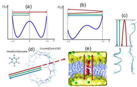
Figure 1: Five systems considered in this paper. The systems are (a) a symmetric 1D potential, (b) symmetric 1D system, (c) deca-alanine, and (d) host-guest complex of CB7 and hexafluorobenzene, and (e) gramicidin A (red ribbon) inserted in a lipid bilayer (blue lines). In (e), water is represented by the yellow surface and potassium ions by green balls. Forward (green), reverse (blue), and symmetric (red) processes are shown with colored arrows.

III.2 Nonequilibrium Pulling Simulations

For the first four systems, we performed simulations with a forward, reverse, and symmetric process. For gA, we analyzed the symmetric simulations from Ngo et al. (2016).

For the 1D potential energy surfaces, Brownian dynamics simulations were performed using an in-house python script. For the symmetric potential, the symmetric process consisted of pulling the Brownian particle at a constant speed from the equilibrated state at $\lambda=-1.5$ to $\lambda=1.5$ in 750 steps. In the forward asymmetric process, it was pulled from the equilibrated state at $\lambda=-1.5$ to $\lambda=0$. In the reverse process, it was pulled from the equilibrated state at $\lambda=0$ to $\lambda=-1.5$ in 375 steps (Figure 1a). For the asymmetric potential, the symmetric process consisted of pulling the particle from the equilibrated state at $\lambda=-1.5$ to $\lambda=1.5$ and (without equilibrating) back to $\lambda=-1.5$ in 1500 steps. In the forward asymmetric process, it was pulled from the equilibrated state at $\lambda=-1.5$ to $\lambda=1.5$. In the reverse, it was pulled from the equilibrated state at $\lambda=1.5$ to $\lambda=-1.5$ in 750 steps (Figure 1b). The force constant $k$ of the pulling harmonic potential was chosen to be $k=15$ units of energy per one unit of length squared (for the 1D systems, distance, time, and energy have no specified unit). For each system, we collected 20,000 pulling trajectories for the symmetric process and 40,000 for the asymmetric process. Each set of trajectories was partitioned into 100 blocks.

For deca-alanine and the host-guest complex, Langevin dynamics simulations were performed using NAMD 2.9 Phillips et al. (2005). The systems were in vacuum. Bond distances involving hydrogen atoms were constrained using the SHAKE algorithm Smith and Dang (1994) which enabled the use of a time step of 2 fs. Nonbonded cutoffs were set to 999 Å. At each end state the structures were minimized for 1000 steps and the temperature was increased by 10 K every 100 steps from 0 to 300 K. After discarding the first 100 ps, equilibrated structures were collected every 1 ps over a total production time of 1 ns at at 300 K.

With deca-alanine, one end of the peptide was fixed and the other end was attached to the harmonic potential $V(d,t)$, where $d$ is the distance between the two ends. The force constant was set to $k=7.2$ kcal/mol/Ų, which is the same as in a previous paper Park et al. (2003). The peptide was equilibrated at both $\lambda=1.3$ nm and $\lambda=3.3$ nm for 1 ns. In the symmetric process, the spring was pulled from the equilibrated state at $\lambda=1.3$ nm to 3.3 nm and, without equilibrating, compressed it back to 1.3 nm. In the forward asymmetric process, it was pulled from the equilibrated state at $\lambda=1.3$ nm to 3.3 nm, while in the reverse counterpart it was pulled from the equilibrated state at $\lambda=3.3$ nm to 1.3 nm. The pulling speed for all the processes was set to 2 nm per 1 ns. We collected 200, 400, and 400 trajectories for the symmetric, forward, and reverse asymmetric processes, respectively. Each set of trajectories was partitioned into 10 blocks.

With the host-guest complex, the harmonic pulling potential $V(z,t)$ was attached to the center of mass of the guest molecule and $\lambda$ was set to the $z$ coordinate of harmonic trap position. The spring constant was chosen as $k=7.2$ kcal/mol/Ų, which is the same as for deca-alanine. The complex was equilibrated at both $\lambda=-2$ nm and $\lambda=0$ nm for 1 ns. In the symmetric process, the spring pulled the guest molecule from the equilibrated state at $\lambda=-2$ nm through the pore of the host to $\lambda=2$ nm. In the forward asymmetric process, it was pulled from the equilibrated state at $\lambda=-2$ nm to the center of the host at $\lambda=0$ nm. In its reverse counterpart, the spring was pulled from the equilibrated state at $\lambda=0$ nm to $\lambda=-2$ nm (Figure 1d). The pulling speed was the same for all processes and set to 2.5 nm per ns. We collected 400, 800 and 800 trajectories for the symmetric, forward and reverse processes, respectively. Each set of trajectories was partitioned into 10 blocks.

In the pulling simulations described in Ngo et al. (2016), the potassium ion was pulled from $z=-1.3$ nm to $z=1.3$ nm using a harmonic force constant of $k=100$ kcal/mol/Ų. Two pulling speeds were used, $v=100$ Å/ns and $v=10$ Å/ns. For the fast pulling simulations, 145 forward (pulling from $z=-1.3$ nm to $z=1.3$ nm) and 145 reverse (from $z=1.3$ nm to $z=-1.3$ nm) trajectories were collected. For the slow pulling simulations, the number of trajectories collected were 16 for forward and 16 for reverse pulling.

III.3 Reference free energies and PMFs

For the 1D potentials, reference values were based on numerical integration and from the exact PMF. The exact PMF is simply the potential itself. The reference free energy was computed by numerically integrating $F_{t}=\int e^{-\beta\left[U(z)+V(z,t)\right]}dz$ between $\lambda(t)-5<z<\lambda(t)+5$, where $U(z)$ is $U^{\textrm{sym}}(z)$ or $U^{\textrm{asym}}(z)$, using the adaptive quadrature method implemented in SciPy 0.17.0.

For the other systems, reference free energies and PMFs were based on umbrella sampling and WHAM. For deca-alanine, umbrella sampling was based on 100 windows which were equally spaced between $\lambda=1.3$ nm and $\lambda=3.3$ nm. For the host-guest complex, we used 200 windows equally spaced between $\lambda=-2$ nm and $\lambda=2$ nm. In each window, we equilibrated for 1 ns and ran production simulation for 20 ns. The spring constant was set to $k=7.2$ kcal/mol/Ų, which is the same as in the nonequilibrium pulling simulations. As in the pulling processes, Langevin dynamics simulations at 300 K of each system in vacuum were performed using NAMD 2.9 Phillips et al. (2005) with a time step of 2 fs. In the gA system, umbrella sampling was carried out in Ngo et al. (2016) using 49 windows equally spaced between $z=-1.2$ nm and $z=1.2$ nm.

We used the multistate Bennett acceptance ratio Shirts and Chodera (2008) (MBAR) to estimate the free energy differences and the weighted histogram analysis method Ferrenberg and Swendsen (1989); Kumar et al. (1992) (WHAM) to estimate PMFs.

III.4 Analysis

In the first four systems, the nonequilibrium work data generated by three processes — forward (f), reverse (r), and symmetric (s) — was combined with three estimators — unidirectional (u), bidirectional (b) and symmetric (s) — to produce six different estimates of the free energy and PMF. For symmetric processes, the generated data were used with all three estimators to give three estimates: s_u, s_b and s_s. When using the bidirectional estimator, we split the total set of data into two halves, considering the first half as forward and the second as reverse because the symmetric process is both forward and reverse. For asymmetric (forward and reverse) processes, we applied the unidirectional estimator to each direction to produce f_u and r_u estimates and combined both directions using the bidirectional estimator to obtain the fr_b estimate. When asymmetric processes were used in symmetric systems, we exploited the symmetry of the system by replicating free energies and PMFs from one half of the process or system to the other half. To make the comparison of symmetric and asymmetric processes as fair as possible, the fact that asymmetric processes were half the length was compensated for by analyzing twice as many trajectories. For every system, free energy and PMF estimates were generated for each of the 10 or 100 blocks. The estimates were used to calculate the RMSE with respect to reference values.

In gA, nonequilibrium work data were processed with the unidirectional (u), bidirectional (b), symmetric (s) estimators as well as b+WHAM estimator Ngo et al. (2016), which uses bidirectional data to initiate the weighted histogram analysis method.

IV Results

IV.1 1D systems

For the symmetric potential, if work data is generated by a symmetric process, then applying the our new symmetric estimator, Equation 7, gives more accurate free energy and PMF estimates than the previous unidirectional (Equation 8) and bidirectional (Equation 9) estimators. Free energy and PMF estimates from the unidirectional and bidirectional estimators, s_u and s_b, respectively, show large biases in the right half of the potential (Figure 2). The bias in the unidirectional estimator is substantially larger. When using the symmetric estimator (s_s), RMSEs of the free energies and PMFs are significantly reduced.

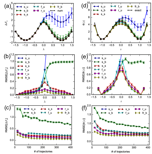
Figure 2: Free energies and PMFs for the symmetric 1D system. Lines are labeled by combining the name of the nonequilibrium process: “s” for symmetric process, “f” for forward, and “r” for reverse asymmetric process, with name of the estimator: “u” for unidirectional, “b” for bidirectional (MA) and “s” for symmetric. [(a) and (d)]: Comparison of free energies and PMFs estimated by nonequilibrium path ensemble average estimators with numerical free energy (num) and exact PMF (exact). [(b) and (e)]: RMSE of free energies and PMFs estimated by non-equilibrium path ensemble average estimators with respect to the numerical free energies and exact PMF, respectively. [(c) and (f)]: Convergence of RMSE of free energies and PMFs with the number of non-equilibrium trajectories. RMSEs are averaged over $\lambda$ for free energies or bins for PMFs. For f_u, r_u and fr_u, the actual number of trajectories is double the number shown in panels (c) and (f). In panels (b) and (e), RMSEs greater than 1.2 are not shown. In panels (c) and (f), s_u lines are larger than 1.5 and 2, respectively, and are not shown.

Although the symmetric estimator leads to the best performance when analyzing data from symmetric processes, better performance is achieved with data from asymmetric processes. The lowest RMSEs for both free energies and PMFs are obtained when applying the bidirectional estimator to asymmetric processes. When using the unidirectional estimator, the RMSEs depend quite significantly on the direction of pulling, e.g. forward from $\lambda=-1.5$ to 0 or reverse from $\lambda=0$ to -1.5. For this system, r_u gives much lower RMSEs than f_u, especially around the barrier region of the 1D potential (Figure 2). Free energy and PMF estimates from our new symmetric estimator s_s have lower RMSEs than r_u but larger RMSEs than r_u and fr_b, although the difference is less significant for the PMFs.

The fr_b estimates show the fastest convergence with respect to the number of trajectories (Figures 2c and f). The convergence of our new estimator s_s is slightly slower than r_u and faster than f_u. Both s_u and s_b show extremely slow convergence (s_u is not shown because it is out of range).

Similar trends hold for the asymmetric 1D potential. s_s is the best of estimators for symmetric processes, but fr_b has the best performance overall. For all estimators except fr_b, there is significant bias in the region to the right of $z=0$. s_u estimates of free energies and PMFs have the largest RMSEs (Figure 3). Unlike the symmetric system above, the bidirectional estimator combined with symmetric process (s_b) gives almost identical performance to our new symmetric estimator (s_s). The forward asymmetric process from $\lambda=-1.5$ to $\lambda=1.5$ (f_u) is better than the reverse counterpart (r_u) and is nearly identical to s_s. fr_b estimates show the fastest convergence with respect to the number of trajectories. All other estimators except for s_u, which is particularly slow, converge at a similar rate.

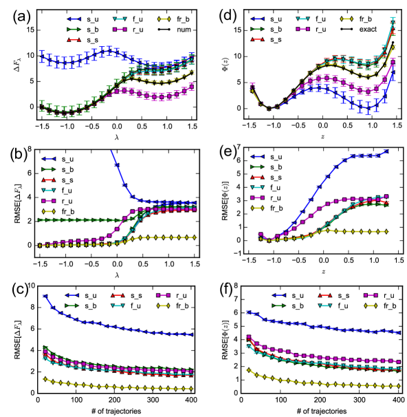
Figure 3: Free energies and PMFs for the asymmetric 1D system. Lines are labeled by combining the name of the nonequilibrium process: “s” for symmetric process, “f” for forward, and “r” for reverse asymmetric process, with name of the estimator: “u” for unidirectional, “b” for bidirectional (MA) and “s” for symmetric. [(a) and (d)]: Comparison of free energies and PMFs estimated by nonequilibrium path ensemble average estimators with numerical free energy (num) and exact PMF (exact). [(b) and (e)]: RMSE of free energies and PMFs estimated by non-equilibrium path ensemble average estimators with respect to the numerical free energies and exact PMF, respectively. [(c) and (f)]: Convergence of RMSE of free energies and PMFs with the number of non-equilibrium trajectories. RMSEs are averaged over $\lambda$ for free energies or bins for PMFs. For f_u, r_u and fr_u, the actual number of trajectories is double the number shown in panels (c) and (f). In (b), free energy RMSEs larger than 8 are not shown.

IV.2 Deca-alanine

The performance of estimators for deca-alanine is distinct from the 1D potentials (Figure 4). In particular, fr_b has especially weak performance, especially when $\lambda$ or $d$ are near 2 nm. In its place, s_s and f_u are the best estimators, with comparably low RMSEs and convergence properties for both free energies and PMFs. Remarkably, s_u, which shows the worst performance for the 1D systems, gives rather low RMSE for the PMFs (Figure 4) and the RMSE decreases dramatically with the number of trajectories (Figures 4c and f). Among the estimates arising from the asymmetric processes, f_u gives the lowest RMSEs for both free energies and PMFs whereas r_u and fr_b give significantly larger RMSEs. In this case, the reverse pulling is extremely unhelpful and combining it with the forward counterpart using the bidirectional estimator does not improve free energy estimates.

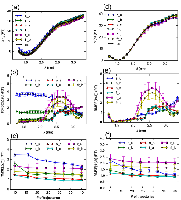
Figure 4: Free energies and PMFs for deca-alanine. Lines are labeled by combining the name of the nonequilibrium process: “s” for symmetric process, “f” for forward, and “r” for reverse asymmetric process, with name of the estimator: “u” for unidirectional, “b” for bidirectional (MA) and “s” for symmetric. [(a) and (d)]: Comparison of free energies and PMFs estimated by nonequilibrium path ensemble average estimators with numerical free energy (num) and exact PMF (exact). [(b) and (e)]: RMSE of free energies and PMFs estimated by non-equilibrium path ensemble average estimators with respect to the numerical free energies and exact PMF, respectively. [(c) and (f)]: Convergence of RMSE of free energies and PMFs with the number of non-equilibrium trajectories. RMSEs are averaged over $\lambda$ for free energies or bins for PMFs. For f_u, r_u and fr_u, the actual number of trajectories is double the number shown in panels (c) and (f).

IV.3 Host-guest complex

Free energy estimates in the host-guest complex are notable because of much larger error inside versus outside of the host (Figure 5). As in most systems, s_s is the best of estimates based on symmetric protocols and fr_b has the lowest RMSE overall. f_u has a similar performance to s_s. The s_u estimates of free energies and PMFs again have the largest RMSEs, especially on the right half of the free energy and PMF. In all estimators except for r_u and fr_b, free energies and PMFs are overestimated inside of the host. In fr_b, the quantities are slightly underestimated. In r_u, the underestimation is much more significant.

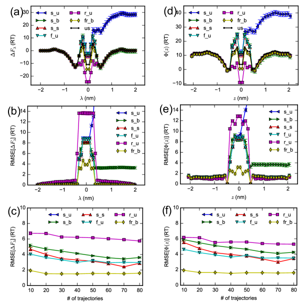
Figure 5: Free energies and PMFs for host-guest complex. Lines are labeled by combining the name of the nonequilibrium process: “s” for symmetric process, “f” for forward, and “r” for reverse asymmetric process, with name of the estimator: “u” for unidirectional, “b” for bidirectional (MA) and “s” for symmetric. [(a) and (d)]: Comparison of free energies and PMFs estimated by nonequilibrium path ensemble average estimators with numerical free energy (num) and exact PMF (exact). [(b) and (e)]: RMSE of free energies and PMFs estimated by non-equilibrium path ensemble average estimators with respect to the numerical free energies and exact PMF, respectively. [(c) and (f)]: Convergence of RMSE of free energies and PMFs with the number of non-equilibrium trajectories. RMSEs are averaged over $\lambda$ for free energies or bins for PMFs. For f_u, r_u and fr_u, the actual number of trajectories is double the number shown in panels (c) and (f). In panels (b) and (e), RMSEs larger than 15 RT are not shown.

IV.4 Gramicidin A

Depending on the pulling speed, Equation 7 (s) leads to either the most accurate or second most accurate PMF estimates. For the fast pulling speed, the b+WHAM estimate is the least biased (Figure 6a). Equation 7 (s) is less accurate than b+WHAM, with the largest bias occurring near the energy barrier. On the other hand, Equation 8 (u) and Equation 9 (b) show significant bias, especially on the right side of the energy barrier. When the pulling is slow (Figure 6b), Equation 7 (s) leads to the most accurate PMF estimates, most accurately reproducing the shape of the barrier. On the other hand, b+WHAM is slightly biased. As with the fast pulling, Equation 8 (u) and Equation 9 (b) are highly biased on the right side, when $z>0$.

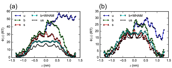
Figure 6: PMFs for gA. The pulling speed is (a) $v=100$ Å/ns and (b) $v=10$ Å/ns. Comparison of PMFs from unidirectional (u), bidirectional (b), symmetric (s), combined bidirectional and WHAM (b+WHAM), and umbrella sampling (us).

V Discussion

Demonstrative calculations on 1D potentials and molecular systems show that if work data are generated by a symmetric process, it is always best to use our newly derived symmetric estimator (s_s). The symmetric estimator gives lower RMSEs compared to unidirectional (s_u) and bidirectional (s_b) estimators. On the other hand, if they are generated from a pair of asymmetric processes, the bidirectional estimator (fr_b) usually gives the lowest overall RMSEs.

The host-guest complex illustrates the benefits of using a bidirectional estimator. The trajectories of nonequilibrium driven processes that are most useful for reconstructing equilibrium properties are close to equilibrium. When using only the forward process of inserting the guest into the host (f_u), the barrier to insertion is accurately determined but the depth of the well in the bound complex, which is farthest from the initial state, is not low enough. On the other hand, when only using the reverse process of extracting the guest (r_u), the bound state is close to equilibrium and the well depth appears to be accurate. When the complex starts to dissociate, however, the system fails to form interactions that would reduce the work and lead to a smaller barrier to extraction, so the overall well depth is too low.

Although bidirectional estimation generally has better performance, there appears to be an exception if one process is much further from equilibrium than its counterpart, as in deca-alanine. In this system, the forward process involves unfolding of the peptide and the reverse process corresponds to refolding a helix from an extended state. Due to a large number of structural rearrangements required for refolding, the system is unlikely to find the native conformation during reverse process. Hence, estimates from the reverse process are biased and r_u has a large RMSE. Due to the relatively far-from-equilibrium nature of reverse trajectories, the bidirectional estimator has worse performance than f_u.

In addition to cases where one direction is further from equilibrium than its counterpart, the bidirectional estimator has the disadvantage that the system needs to be equilibrated at both ends. This may not always be feasible. In a simulation, equilibration consumes more computer time. In a single-molecule pulling experiment, waiting for equilibration can accumulate more drift.

In situations where a bidirectional process is not feasible or beneficial, a symmetric protocol and Equation 7 is an attractive alternative to a unidirectional process and analysis; it can significantly reduce the experimental measurement or computer simulation time required to attain the same accuracy. For example, in a single-molecule pulling experiment, a forward protocol that unfolds a molecule can be immediately followed by its time reversal to create a symmetric protocol. As the performance of s_s and f_u for the same amount of simulation time are remarkably similar, our results suggest that using a symmetric protocol to return to the initial position of the apparatus before equilibration is as valuable as collecting data from twice as many forward processes alone. In contrast to using only forward processes, however, the symmetric protocol reduces the time in equilibration and makes use of data from the return to the initial apparatus position. As another example, simulating the pulling of a small organic molecule completely across a symmetric lipid membrane and using Equation 7 could be useful for membrane permeability studies. In this case, it can be significantly more difficult to equilibrate the molecule in the middle of the membrane than in the solvent. If the small molecule is pulled completely through the membrane using a symmetric protocol, our data suggest that Equation 7 will yield more accurate results than the unidirectional estimator, Equation 8.

There are several tradeoffs in the choice between b+WHAM and the symmetric estimator, Equation 7. On one hand, gA simulations suggest that b+WHAM is more capable of reducing bias when estimating equilibrium properties using far-from-equilibrium trajectories. On the other hand, the symmetric estimator is more theoretically rigorous because it does not assume that configurations are drawn from equilibrium distributions (an assumption in WHAM). Consequently, it appears to reconstruct the shape of PMFs more accurately. Figure 6 also highlights the importance of selecting an appropriate pulling speed. Regardless of the estimator, PMFs reconstructed from the processes that are closer to equilibrium are more accurate than those from the faster pullings.

VI Conclusions

We have developed a new and theoretically rigorous statistical estimator for estimating nonequilbrium path-ensemble averages for driven processes with symmetric protocols. In demonstrative calculations, the symmetric estimator outperforms existing rigorous estimators when using such trajectories to estimate free energies and PMFs. If bidirectional trajectories initiated from two equilibrated states are available, however, they usually outperform the symmetric estimator. Hence, we only recommend using symmetric protocols and the new estimator in situations where the bidirectional approach is not practical or expected to be beneficial. Results from the symmetric estimator are remarkably similar to those from twice as many forward process that constitute the first half of the symmetric protocol.