Semilocal exchange-correlation potentials for solid-state calculations: Current status and future directions

Abstract

Kohn-Sham (KS) density functional theory (DFT) is a very efficient method for calculating various properties of solids as, for instance, the total energy, the electron density, or the electronic band structure. The KS-DFT method leads to rather fast calculations, however the accuracy depends crucially on the chosen approximation for the exchange and correlation (xc) functional $E_{\text{xc}}$ and/or potential $v_{\text{xc}}$. Here, an overview of xc methods to calculate the electronic band structure is given, with the focus on the so-called semilocal methods that are the fastest in KS-DFT and allow to treat systems containing up to thousands of atoms. Among them, there is the modified Becke-Johnson potential that is widely used to calculate the fundamental band gap of semiconductors and insulators. The accuracy for other properties like the magnetic moment or the electron density, that are also determined directly by $v_{\text{xc}}$, is also discussed.

I Introduction

The calculation of the properties of solids can be done very efficiently with the Kohn-ShamKohn and Sham (1965) (KS) method of density functional theoryHohenberg and Kohn (1964) (DFT). KS-DFT is clearly much faster than other methods, like for instance $GW$,Hedin (1965); Aryasetiawan and Gunnarsson (1998) that are commonly used for calculating the quasiparticle band structure, or the random-phase approximation (RPA) and beyondRen et al. (2013); Chen et al. (2017) for the total energy. Therefore, KS-DFT calculations on solids with a unit cell containing up to several thousands of atoms can be afforded. However, in KS-DFT a component in the total energy expression and in the effective potential in the corresponding KS equations, the one accounting for the exchange (x) and correlation (c) effects, has to be approximated. Exchange is due to the Pauli exclusion principle, while correlation arises due to a lowering of the energy by considering wavefunctions that are beyond the single determinant approximation in the Hartree-Fock theory. Since the reliability of the results obtained with KS-DFT depends mainly on the chosen xc functional, the search for more accurate approximate functionals is a very active field of researchKümmel and Kronik (2008); Cohen, Mori-Sánchez, and Yang (2012); Mardirossian and Head-Gordon (2017) and several hundreds have been proposed so far.Lehtola et al. (2018); Mardirossian and Head-Gordon (2017) Most xc-functionals can be classified on the Jacob’s ladder of John Perdew,Perdew and Schmidt (2001); Perdew et al. (2005) where the first rung represents the most simple type of approximations and the highest rung the most sophisticated functionals. The rather general rule is that the functionals should, in principle, be more accurate, but also (this is the downside) computationally more expensive to evaluate when climbing up Jacob’s ladder.

The properties of solids which are calculated directly from total energy are for instance the equilibrium geometry, the cohesive energy, or the formation enthalpy. For such calculations, a couple of xc functionals Perdew et al. (1992); Perdew, Burke, and Ernzerhof (1996); Heyd, Scuseria, and Ernzerhof (2003); Wu and Cohen (2006); Perdew et al. (2008); Sun, Ruzsinszky, and Perdew (2015) were or are considered as standard. Other properties depend more directly on the accuracy of the xc potential in the KS equations, such as the electronic band structure, the electron density, and magnetism, for which it may sometimes be necessary to use other types of xc approximations Anisimov, Zaanen, and Andersen (1991); Heyd, Scuseria, and Ernzerhof (2003); Tran and Blaha (2009); Kuisma et al. (2010) to get reliable results.

Here, the focus will be on the calculation of the electronic band structure of semiconductors and insulators with xc methods that are computationally the fastest, namely the so-called semilocal methods. Needless to say that quantities derived from the electronic band structure such as the band gap or the optical constants can serve as a guide for the design of more efficient materials for technological applications like photovoltaics,Yu and Zunger (2012); Ong et al. (2019) light emitting diodes,Xiao et al. (2017); Mitchell et al. (2018) dynamic random access memory,Traversa et al. (2014) or thermoelectricity.Urban et al. (2019) Among the semilocal methods, the modified Becke-Johnson potential proposed by two of usTran and Blaha (2009) has been shown to be very accurate for the calculation of the fundamental band gap. Comparison studies for the band gap (see Refs. Lee et al., 2016; Tran and Blaha, 2017; Pandey, Kuhar, and Jacobsen, 2017; Nakano and Sakai, 2018; Tran, Ehsan, and Blaha, 2018; Borlido et al., 2019 for the most exhaustive comparisons) have shown that the modified Becke-Johnson potential is on average more accurate than basically all other DFT methods, including the traditional hybrid functionals using a fixed fraction of Hartree-Fock exchange. Presently, only dielectric-function-dependent hybrid functionalsMarques et al. (2011); Koller, Blaha, and Tran (2013); Skone, Govoni, and Galli (2014); Chen et al. (2018) and $GW$ methods, in particular if applied self-consistently including vertex corrections,Shishkin, Marsman, and Kresse (2007); Chen and Pasquarello (2015) can lead to higher accuracy. However, since the modified Becke-Johnson potential is a DFT method, and furthermore was constructed empirically, the results are of course not systematically accurate. In addition, making a xc method accurate for a specific property (e.g., band gap), may deteriorate the description of other properties compared to more traditional methods.

The remainder of this paper is organized as follows. In Sec. II, a brief introduction to the KS-DFT method is given and the existing approximations for the xc potential $v_{\text{xc}}$ are reviewed. Then, Sec. III provides a summary of the performance of various potentials for the electronic structure with a particular emphasis on the fundamental band gap. Results for other properties, e.g., the bandwidth, the magnetic moment, or the electron density, will also be mentioned. Finally, a summary is given in Sec. IV and ideas for further improvements are given in Sec. V.

II Theoretical background

II.1 (Generalized) Kohn-Sham equations

In the KS-DFT method,Kohn and Sham (1965) the total energy per unit cell of a periodic solid is given by

$$E_{\text{tot}}=T_{\text{s}}+\frac{1}{2}\int\limits_{\text{cell}}v_{\text{Coul}}(\mathbf{r})\rho(\mathbf{r})d^{3}r-\frac{1}{2}\sum_{\alpha}^{\text{cell}}Z_{\alpha}v_{\text{M}}^{\alpha}(\mathbf{R}_{\alpha})+E_{\text{xc}},$$ (1)

where

$$T_{\text{s}}=-\frac{1}{2}\sum_{\sigma}\sum_{n,\mathbf{k}}w_{n\mathbf{k}\sigma}\int\limits_{\text{cell}}\psi_{n\mathbf{k}\sigma}^{*}(\mathbf{r})\nabla^{2}\psi_{n\mathbf{k}\sigma}(\mathbf{r})d^{3}r$$ (2)

is the noninteracting kinetic energy, the second and third terms represent the electrostatic interactions (electron-electron, electron-nucleus, and nucleus-nucleus) with

$$v_{\text{Coul}}(\mathbf{r})=\int\limits_{\text{crystal}}\frac{\rho(\mathbf{r}^{\prime})}{\left|\mathbf{r}-\mathbf{r}^{\prime}\right|}d^{3}r^{\prime}-\sum_{\beta}^{\text{crystal}}\frac{Z_{\beta}}{\left|\mathbf{r}-\mathbf{R}_{\beta}\right|}$$ (3)

and

$$v_{\text{M}}^{\alpha}(\mathbf{R}_{\alpha})=\int\limits_{\text{crystal}}\frac{\rho(\mathbf{r}^{\prime})}{\left|\mathbf{R}_{\alpha}-\mathbf{r}^{\prime}\right|}d^{3}r^{\prime}-\sum_{\beta\atop\beta\neq\alpha}^{\text{crystal}}\frac{Z_{\beta}}{\left|\mathbf{R}_{\alpha}-\mathbf{R}_{\beta}\right|}$$ (4)

being the Coulomb and Madelung potentials, respectively, and $E_{\text{xc}}$ is the exchange-correlation energy. In Eqs. (1), (3), and (4), $\rho=\rho_{\uparrow}+\rho_{\downarrow}$ is the electron density, while $Z_{\alpha}$ and $\mathbf{R}_{\alpha}$ are the charge and position of the nuclei. In Eq. (2), $n$, $\mathbf{k}$, and $\sigma$ are the band index, $\mathbf{k}$-point, and spin index, respectively, and $w_{n\mathbf{k}\sigma}$ is the product of the $\mathbf{k}$-point weight and the occupation number.

Searching for the Slater determinant which minimizes Eq. (1) yields the one-electron Schrödinger equations

$$\left(-\frac{1}{2}\nabla^{2}+v_{\text{Coul}}(\mathbf{r})+\hat{v}_{\text{xc},\sigma}(\mathbf{r})\right)\psi_{n\mathbf{k}\sigma}(\mathbf{r})=\varepsilon_{n\mathbf{k}\sigma}\psi_{n\mathbf{k}\sigma}(\mathbf{r})$$ (5)

that need to be solved self-consistently together with $\rho_{\sigma}=\sum_{n,\mathbf{k}}w_{n\mathbf{k}\sigma}\left|\psi_{n\mathbf{k}\sigma}\right|^{2}$. Within the strict KS framework, $\hat{v}_{\text{xc},\sigma}$ is calculated as the functional derivative of $E_{\text{xc}}$ with respect to the electron density $\rho_{\sigma}$ ($\hat{v}_{\text{xc},\sigma}=\delta E_{\text{xc}}/\delta\rho_{\sigma}$), which means that $\hat{v}_{\text{xc},\sigma}$ is a multiplicative potential ($\hat{v}_{\text{xc}}\psi_{n\mathbf{k}\sigma}=v_{\text{xc}}\psi_{n\mathbf{k}\sigma}$), i.e., it is the same for all orbitals. Instead, in the generalized KS (gKS) framework,Seidl et al. (1996) the derivative of $E_{\text{xc}}$ is taken with respect to $\psi_{n\mathbf{k}\sigma}^{*}$ ($\hat{v}_{\text{xc}}\psi_{n\mathbf{k}\sigma}=\delta E_{\text{xc}}/\delta\psi_{n\mathbf{k}\sigma}^{*}$), which leads to a non-multiplicative xc operator (i.e., a potential that is different for each orbital $\psi_{n\mathbf{k}\sigma}$) in the case of functionals $E_{\text{xc}}$ that do not depend only explicitly on $\rho_{\sigma}$.

Functionals whose $\rho_{\sigma}$-dependency is fully explicit are, for instance, the local density approximation (LDA)Kohn and Sham (1965) and generalized gradient approximations (GGA). The most known examples of functionals that depend implicitly on $\rho_{\sigma}$ are Hartree-Fock (HF) and the meta-GGAs (MGGA).Della Sala, Fabiano, and Constantin (2016)

As mentioned above, there are two types of xc potentials: multiplicative and non-multiplicative. In addition, among the multiplicative potentials $v_{\text{xc},\sigma}$ there are two distinctive subgroups, namely, those which are functional derivatives $v_{\text{xc},\sigma}=\delta E_{\text{xc}}/\delta\rho_{\sigma}$ of an energy functional $E_{\text{xc}}$ and those which are not, but were modelled directly. Among the non-multiplicative potentials, the only ones we are aware of that are not obtained as functional derivative $\hat{v}_{\text{xc}}\psi_{n\mathbf{k}\sigma}=\delta E_{\text{xc}}/\delta\psi_{n\mathbf{k}\sigma}^{*}$ are the hybrids with a fraction of HF exchange that depends on a property of the system like the dielectric function (see, e.g. Refs. Marques et al., 2011; Koller, Blaha, and Tran, 2013; Skone, Govoni, and Galli, 2014). The two next sections list some of the potentials which are the most relevant for the present work, i.e., for band gaps in particular. Then, in the third section a summary of what is known about the xc derivative discontinuity, which is strongly related to the band gap, is provided. Actually, we mention that we are here concerned with calculated band gaps that are obtained with the orbital energies, see Sec. II.4 for more discussion.

II.2 Multiplicative potentials

II.2.1 Potentials that are functional derivatives

We start by defining the xc-energy density per volume $\varepsilon_{\text{xc}}$,

$$E_{\text{xc}}=\int\limits_{\text{cell}}\varepsilon_{\text{xc}}(\mathbf{r})d^{3}r,$$ (6)

which in LDA is a function of $\rho_{\sigma}$:

$$\varepsilon_{\text{xc}}^{\text{LDA}}(\mathbf{r})=\varepsilon_{\text{xc}}^{\text{LDA}}\left(\rho_{\uparrow}(\mathbf{r}),\rho_{\downarrow}(\mathbf{r})\right),$$ (7)

while in GGABecke (1988); Perdew, Burke, and Ernzerhof (1996) the first derivative of $\rho_{\sigma}$ is also used:

$$\varepsilon_{\text{xc}}^{\text{GGA}}(\mathbf{r})=\varepsilon_{\text{xc}}^{\text{GGA}}\left(\rho_{\uparrow}(\mathbf{r}),\rho_{\downarrow}(\mathbf{r}),\nabla\rho_{\uparrow}(\mathbf{r}),\nabla\rho_{\downarrow}(\mathbf{r})\right).$$ (8)

The functional derivative of LDA and GGA functionals is straightforwardly calculated with Parr and Yang (1989)

$$v_{\text{xc},\sigma}^{\text{LDA}}=\frac{\delta E_{\text{xc}}^{\text{LDA}}}{\delta\rho_{\sigma}}=\frac{\partial\varepsilon_{\text{xc}}^{\text{LDA}}}{\partial\rho_{\sigma}}$$ (9)

and

$$v_{\text{xc},\sigma}^{\text{GGA}}=\frac{\delta E_{\text{xc}}^{\text{GGA}}}{\delta\rho_{\sigma}}=\frac{\partial\varepsilon_{\text{xc}}^{\text{GGA}}}{\partial\rho_{\sigma}}-\nabla\cdot\left(\frac{\partial\varepsilon_{\text{xc}}^{\text{GGA}}}{\partial\nabla\rho_{\sigma}}\right),$$ (10)

respectively. From Eqs. (9) and (10), we can see that a GGA potential depends on $\rho_{\sigma}$ and the first and second derivatives of $\rho_{\sigma}$, while $v_{\text{xc},\sigma}^{\text{LDA}}$ depends only on $\rho_{\sigma}$.

Among the functionals $E_{\text{xc}}$ of the LDA type that will be considered for the discussion in Sec. III, there is the functional of the homogeneous electron gasKohn and Sham (1965); Vosko, Wilk, and Nusair (1980); Perdew and Wang (1992) (called LDA) and SlocFinzel and Baranov (2017) (local Slater potential), which is an enhanced exchange LDA with no correlation and was proposed specifically for band gap calculations.

With something like 200 functionals, the GGAs represent the largest group of functionals,Lehtola et al. (2018) however only a couple of them were shown to be interesting for the band gap. Among them, the three following are here considered. EV93PW91, which consists of the exchange EV93 of Engel and VoskoEngel and Vosko (1993) that we combined with PW91 correlationPerdew et al. (1992) in our previous works.Tran, Blaha, and Schwarz (2007); Tran and Blaha (2017) The EV93 exchange was constructed to reproduce the exact exchange (EXX) potential in atoms. AK13 from Armiento and Kümmel,Armiento and Kümmel (2013) a parameter-free exchange functional that was constructed to have a potential that changes discontinuously at integer particle numbers. In our previous works,Tran and Blaha (2017) as well as in others,Vlček et al. (2015) AK13 was used with no correlation added. In the recently proposed GGA HLE16,Verma and Truhlar (2017a) the parameters were tuned in order to give accurate band gaps. Of course, the standard GGA for solids of Perdew et al.Perdew, Burke, and Ernzerhof (1996) (PBE), which is known to be very inaccurate for band gaps,Heyd et al. (2005) will also be considered [note that a simple relationship between PBE and one-shot $GW$ ($G_{0}W_{0}$) band gaps was proposed in Ref. Morales-García, Valero, and Illas, 2017]. Other standard GGAs like BLYPBecke (1988); Lee, Yang, and Parr (1988) or PBEsolPerdew et al. (2008) lead to results for the electronic structure that are very similar to PBETran et al. (2015) and, therefore, do not need to be considered.

The other families of pure DFT approximations for $E_{\text{xc}}$ like the $\nabla^{2}\rho$-MGGA functionalsDella Sala, Fabiano, and Constantin (2016) which depend on the second derivative of $\rho$, the nonlocal van der Waals functionals,Dion et al. (2004) or the weighted-density approximation Gunnarsson, Jonson, and Lundqvist (1977); Alonso and Girifalco (1978) are not considered in the present work. We just mention that the latter two approximations are more complicated since $\varepsilon_{\text{xc}}$ is itself an integral:

$$\varepsilon_{\text{xc}}(\mathbf{r})=\int\limits_{\text{crystal}}f\left(\rho(\mathbf{r}),\rho(\mathbf{r}^{\prime}),\nabla\rho(\mathbf{r}),\nabla\rho(\mathbf{r}^{\prime}),\left|\mathbf{r}-\mathbf{r}^{\prime}\right|\right)d^{3}r^{\prime},$$ (11)

which brings full nonlocality (they are beyond the semilocal approximations), but also leads to more complicated implementations and expensive calculations.

II.2.2 Potentials that are not functional derivatives

A couple of potentials $v_{\text{xc}}$ were directly modelled in order to produce accurate results for a given property, typically related to the electronic structure, like the band gap. Such potentials having no associated energy functional $E_{\text{xc}}$ were named stray by Gaiduk et al.Gaiduk, Chulkov, and Staroverov (2009)

Presenting such potentials chronologically, we start with LB94,van Leeuwen and Baerends (1994) which reads

$$v_{\text{xc},\sigma}^{\text{LB94}}(\mathbf{r})=v_{\text{xc},\sigma}^{\text{LDA}}(\mathbf{r})-\beta\rho_{\sigma}^{1/3}(\mathbf{r})\frac{y_{\sigma}^{2}(\mathbf{r})}{1+3\beta y_{\sigma}(\mathbf{r})\text{arcsinh}(y_{\sigma}(\mathbf{r}))},$$ (12)

where $y_{\sigma}=\left|\nabla\rho_{\sigma}\right|/\rho_{\sigma}^{4/3}$ and $\beta=0.05$. LB94 was constructed such that the asymptotic behavior at $\left|\mathbf{r}\right|\rightarrow\infty$ in finite systems is $-1/\left|\mathbf{r}\right|$ as it should be. Note that in Ref. Schipper et al., 2000, a slight modification of LB94 (LB94$\alpha$) was proposed, where $\beta=0.01$ and the exchange $v_{\text{x},\sigma}^{\text{LDA}}$ is multiplied by $\alpha=1.19$. From Eq. (12), we can see that the LB94 potential depends on the first derivative of $\rho_{\sigma}$, but not on the second derivative like the GGA potentials do.

Becke and JohnsonBecke and Johnson (2006) (BJ) proposed an approximation to the EXX potential in atoms that is given by

$$v_{\text{x},\sigma}^{\text{BJ}}(\mathbf{r})=v_{\text{x},\sigma}^{\text{BR}}(\mathbf{r})+\frac{1}{\pi}\sqrt{\frac{5}{6}}\sqrt{\frac{t_{\sigma}(\mathbf{r})}{\rho_{\sigma}(\mathbf{r})}},$$ (13)

where

$$v_{\text{x},\sigma}^{\text{BR}}(\mathbf{r})=-\frac{1}{b_{\sigma}(\mathbf{r})}\left(1-e^{-x_{\sigma}(\mathbf{r})}-\frac{1}{2}x_{\sigma}(\mathbf{r})e^{-x_{\sigma}(\mathbf{r})}\right)$$ (14)

is the Becke-Roussel (BR) potentialBecke and Roussel (1989) with $x_{\sigma}$ that is obtained by solving a nonlinear equation involving $\rho_{\sigma}$, $\nabla\rho_{\sigma}$, $\nabla^{2}\rho_{\sigma}$, and the kinetic-energy density $t_{\sigma}=\left(1/2\right)\sum_{n,\mathbf{k}}w_{n\mathbf{k}\sigma}\nabla\psi_{n\mathbf{k}\sigma}^{*}\cdot\nabla\psi_{n\mathbf{k}\sigma}$. Then, in Eq. (14) $b_{\sigma}=\left[x_{\sigma}^{3}e^{-x_{\sigma}}/\left(8\pi\rho_{\sigma}\right)\right]^{1/3}$. Note that in Refs. Becke and Roussel, 1989; Becke and Johnson, 2006; Tran, Blaha, and Schwarz, 2015 the BR potential was shown to reproduce very accurately the Slater potential,Slater (1951) which is the hole component of the EXX potential. Since the BJ potential depends on $t_{\sigma}$ it can be considered as a MGGA, although it is somehow abusive since the mathematical structure of $v_{\text{x},\sigma}^{\text{BJ}}$ differs significantly from the true MGGA potentials discussed in Sec. II.3. The BJ potential has attracted a lot of interest and has been studiedTran, Blaha, and Schwarz (2007); Gaiduk and Staroverov (2008); Staroverov (2008); Gaiduk and Staroverov (2009) or modified Armiento, Kümmel, and Körzdörfer (2008); Karolewski, Armiento, and Kümmel (2009); Tran and Blaha (2009); Räsänen, Pittalis, and Proetto (2010); Pittalis, Räsänen, and Proetto (2010); Tran et al. (2015) by a certain number of groups.

In particular, among these variants of the BJ potential there is the aforementioned mBJLDA xc potential that was introduced in Ref. Tran and Blaha, 2009 as an alternative to the expensive $GW$ and hybrid methods for calculating band gaps. mBJLDA consists of a modification of the BJ potential (mBJ) for exchange and LDAVosko, Wilk, and Nusair (1980); Perdew and Wang (1992) for the correlation potential. The mBJ exchange is given by

$$v_{\text{x},\sigma}^{\text{mBJ}}(\mathbf{r})=cv_{\text{x},\sigma}^{\text{BR}}(\mathbf{r})+\left(3c-2\right)\frac{1}{\pi}\sqrt{\frac{5}{6}}\sqrt{\frac{t_{\sigma}(\mathbf{r})}{\rho_{\sigma}(\mathbf{r})}},$$ (15)

where $c$ is a functional of the density and is given by

$$c=\alpha+\beta\sqrt{g},$$ (16)

where

$$g=\frac{1}{V_{\text{cell}}}\int\limits_{\text{cell}}\frac{1}{2}\left(\frac{\left|\nabla\rho^{\uparrow}(\mathbf{r}^{\prime})\right|}{\rho^{\uparrow}(\mathbf{r}^{\prime})}+\frac{\left|\nabla\rho^{\downarrow}(\mathbf{r}^{\prime})\right|}{\rho^{\downarrow}(\mathbf{r}^{\prime})}\right)d^{3}r^{\prime}$$ (17)

is the average of $\left|\nabla\rho_{\sigma}\right|/\rho_{\sigma}$ in the unit cell. It is important to underline that using $g$ brings some kind of nonlocality since the value of $v_{\text{x},\sigma}^{\text{mBJ}}$ at $\mathbf{r}$ depends on $\left|\nabla\rho_{\sigma}\right|/\rho_{\sigma}$ at every point in space (thus, mBJLDA is not strictly speaking a semilocal method). However, this nonlocality is different from the true nonlocality as in Eq. (11) or in the HF method (see Sec. II.3.1), where there is a dependency on the interelectronic distance $\left|\mathbf{r}-\mathbf{r}^{\prime}\right|$. The values of $\alpha$ and $\beta$ in Eq. (16) were determined to be $\alpha=-0.012$ (dimensionless) and $\beta=1.023$ bohr^1/2 by minimizing the mean absolute error of the band gap for a group of solids.Tran and Blaha (2009) Subsequently, other parametrizations for $\alpha$ and $\beta$ have been proposed in Ref. Koller, Tran, and Blaha, 2012 for semiconductors with band gaps smaller than 7 eV or in Refs. Jishi, Ta, and Sharif, 2014; Traoré et al., 2019 for halide perovskites. Note that in the literature, the mBJLDA potential is sometimes called TB-mBJ,Singh (2010a) TB,Bartók and Yates (2019) or TB09,Marques et al. (2011); Marques, Oliveira, and Burnus (2012); Lehtola et al. (2018) which refers to the authors of the method.

A very interesting potential for band gap calculations was proposed by Kuisma et al.Kuisma et al. (2010) Their potential, which is based on the potential proposed by Gritsenko et al.Gritsenko et al. (1995) (GLLB), is given by (SC stands for solid and correlation)

$$v_{\text{xc},\sigma}^{\text{GLLB-SC}}(\mathbf{r}) = 2e_{\text{x},\sigma}^{\text{PBEsol}}(\mathbf{r})+K_{\text{x}}^{\text{LDA}}$$

$$\times\sum_{n,\mathbf{k}}w_{n\mathbf{k}\sigma}\sqrt{\epsilon_{\text{H}}-\epsilon_{n\mathbf{k}\sigma}}\frac{\left|\psi_{n\mathbf{k}\sigma}(\mathbf{r})\right|^{2}}{\rho_{\sigma}(\mathbf{r})}+v_{\text{c},\sigma}^{\text{PBEsol}}(\mathbf{r}),$$

where $e_{\text{x},\sigma}^{\text{PBEsol}}$ is the PBEsol exchange-energy density per spin-$\sigma$ electron [defined by $E_{\text{x}}=\sum_{\sigma}\int_{\text{cell}}e_{\text{x},\sigma}(\mathbf{r})\rho_{\sigma}(\mathbf{r})d^{3}r$], $v_{\text{c},\sigma}^{\text{PBEsol}}=\delta E_{\text{c}}^{\text{PBEsol}}/\delta\rho_{\sigma}$ is the PBEsol correlation potential, and $K_{\text{x}}^{\text{LDA}}=8\sqrt{2}/\left(3\pi^{2}\right)$. The particularity of the GLLB-SC potential is to depend on the orbital energies [$\epsilon_{\text{H}}$ is for the highest occupied one, i.e., at the valence band maximum (VBM)]. It is easy to showBaerends (2017) that the dependency on $\epsilon_{\text{H}}$ in Eq. (LABEL:eq:vxcGLLBSC) leads to the possibility to calculate the exchange part of the derivative discontinuity, that is given by

$$\Delta_{\text{x}}^{\text{GLLB-SC}} = \int\limits_{\text{cell}}\psi_{\text{L}}^{*}(\mathbf{r})\left[\sum_{n,\mathbf{k}}K_{\text{x}}^{\text{LDA}}w_{n\mathbf{k}\sigma_{\text{L}}}\left(\sqrt{\epsilon_{\text{L}}-\epsilon_{n\mathbf{k}\sigma_{\text{L}}}}\right.\right.$$ (19)

$$-\left.\left.\sqrt{\epsilon_{\text{H}}-\epsilon_{n\mathbf{k}\sigma_{\text{L}}}}\right)\frac{\left|\psi_{n\mathbf{k}\sigma_{\text{L}}}(\mathbf{r})\right|^{2}}{\rho_{\sigma_{\text{L}}}(\mathbf{r})}\right]\psi_{\text{L}}(\mathbf{r})d^{3}r,$$

where $\psi_{\text{L}}$ is the lowest unoccupied orbital [conduction band minimum (CBM)] and $\sigma_{\text{L}}$ its spin value.

Among the other computationally fast model potentials proposed in the literature that are not considered in the present work, we mention the exchange potentials of Lembarki et al.Lembarki, Rogemond, and Chermette (1995) and Harbola and Sen,Harbola and Sen (2002, 2002) which, as LB94, depend on $\rho_{\sigma}$ and $\nabla\rho_{\sigma}$. The exchange potential of UmezawaUmezawa (2006) depends on $\rho_{\sigma}$ and $\nabla\rho_{\sigma}$, but also on the Fermi-Amaldi potentialFermi and Amaldi (1934) which depends on the number of electrons $N$ such that its application to solids is unclear. In Ref. Ferreira, Marques, and Teles, 2008, Ferreira et al. proposed the LDA-1/2 method, which improves upon LDA for band gaps. However, the method is not always straightforward to apply and ambiguities may arise depending on the case (see Refs. Xue et al., 2018; Doumont, Tran, and Blaha, 2019). A few other model potentials can be found in the work of Staroverov.Staroverov (2008)

We also mention that stray potentials have undesirable features both at the fundamental and practical level as shown in Refs. Gaiduk and Staroverov, 2009; Gaiduk, Chulkov, and Staroverov, 2009; Karolewski, Armiento, and Kümmel, 2013.

Last but not least, we mention that some of the potentials presented in this section (LB94, BJ, and mBJ) and in the previous one (e.g., AK13) were shown to lead to numerical problems in the asymptotic region far from nuclei in finite systems.Aschebrock, Armiento, and Kümmel (2017a, b)

II.3 Non-multiplicative potentials

II.3.1 Potentials that are functional derivatives

We begin with the MGGA functionals that use the kinetic-energy density $t_{\sigma}$ as additional ingredient compared to the GGAs (here, we do not consider MGGAs which depend on $\nabla^{2}\rho$):

$$\varepsilon_{\text{xc}}^{\text{MGGA}}=\varepsilon_{\text{xc}}^{\text{MGGA}}\left(\rho_{\uparrow},\rho_{\downarrow},\nabla\rho_{\uparrow},\nabla\rho_{\downarrow},t_{\uparrow},t_{\downarrow}\right).$$ (20)

Since there is, via $t_{\sigma}$, an implicit dependency on $\rho_{\sigma}$, the functional derivative of $E_{\text{xc}}^{\text{MGGA}}$ with respect to $\rho_{\sigma}$ can not be calculated (at least not in a straightforward way). Instead, the functional derivative with respect to $\psi_{n\mathbf{k}\sigma}^{*}$ is taken,Neumann, Nobes, and Handy (1996); Arbuznikov and Kaupp (2003) which gives

$$\hat{v}_{\text{xc},\sigma}^{\text{MGGA}}\psi_{n\mathbf{k}\sigma} = \frac{\partial\varepsilon_{\text{xc}}^{\text{MGGA}}}{\partial\rho_{\sigma}}\psi_{n\mathbf{k}\sigma}-\left(\nabla\cdot\frac{\partial\varepsilon_{\text{xc}}^{\text{MGGA}}}{\partial\nabla\rho_{\sigma}}\right)\psi_{n\mathbf{k}\sigma}$$

$$-\frac{1}{2}\nabla\cdot\left(\frac{\partial\varepsilon_{\text{xc}}^{\text{MGGA}}}{\partial t_{\sigma}}\nabla\psi_{n\mathbf{k}\sigma}\right)$$

$$= v_{\text{xc},\sigma}^{\text{GGA-part}}\psi_{n\mathbf{k}\sigma}-\frac{1}{2}\nabla\cdot\left(\frac{\partial\varepsilon_{\text{xc}}^{\text{MGGA}}}{\partial t_{\sigma}}\nabla\psi_{n\mathbf{k}\sigma}\right),$$

where the last term, which is non-multiplicative, arises due to the dependency on $t_{\sigma}$. Among the numerous MGGA functionals that have been proposed,Della Sala, Fabiano, and Constantin (2016) some of them have been shown to improve clearly over the standard PBE for the geometry and energetics of electronic systems. This includes SCANSun, Ruzsinszky, and Perdew (2015) and MVSSun, Perdew, and Ruzsinszky (2015) (tested in Refs. Yang et al., 2016; Jana, Patra, and Samal, 2018 for the band gap), as well as HLE17Verma and Truhlar (2017b) and revM06-L.Wang et al. (2017)

Another class of functionals that lead to a non-multiplicative potential, but not of the semilocal type, is HF and the (screened) hybrid functionals, where a fraction $\alpha_{\text{x}}$ of semilocal exchange is replaced by HF exchange:

$$\varepsilon_{\text{xc}}^{\text{hybrid}}(\mathbf{r})=\varepsilon_{\text{xc}}^{\text{SL}}(\mathbf{r})+\alpha_{\text{x}}\left[\varepsilon_{\text{x}}^{\text{(scr)HF}}(\mathbf{r})-\varepsilon_{\text{x}}^{\text{(scr)SL}}(\mathbf{r})\right],$$ (22)

where

$$\varepsilon_{\text{x}}^{\text{(scr)HF}}(\mathbf{r}) = -\frac{1}{2}\sum_{\sigma}\sum_{n,\mathbf{k}}\sum_{n^{\prime},\mathbf{k}^{\prime}}w_{n\mathbf{k}\sigma}w_{n^{\prime}\mathbf{k}^{\prime}\sigma}\psi_{n\mathbf{k}\sigma}^{*}(\mathbf{r})\psi_{n^{\prime}\mathbf{k}^{\prime}\sigma}(\mathbf{r})$$

$$\times\int\limits_{\text{crystal}}v\left(\left|\mathbf{r}-\mathbf{r}^{\prime}\right|\right)\psi_{n^{\prime}\mathbf{k}^{\prime}\sigma}^{*}(\mathbf{r}^{\prime})\psi_{n\mathbf{k}\sigma}(\mathbf{r}^{\prime})d^{3}r^{\prime},$$

which is a fully nonlocal exchange-energy density. The functional derivative of $E_{\text{x}}^{\text{(scr)HF}}$ with respect to $\psi_{n\mathbf{k}\sigma}^{*}$ is given by

$$\hat{v}_{\text{x},\sigma}^{\text{(scr)HF}}\psi_{n\mathbf{k}\sigma}(\mathbf{r}) = -\sum_{n^{\prime},\mathbf{k}^{\prime}}w_{n^{\prime}\mathbf{k}^{\prime}\sigma}\psi_{n^{\prime}\mathbf{k}^{\prime}\sigma}(\mathbf{r})$$

$$\times\int\limits_{\text{crystal}}v\left(\left|\mathbf{r}-\mathbf{r}^{\prime}\right|\right)\psi_{n^{\prime}\mathbf{k}^{\prime}\sigma}^{*}(\mathbf{r^{\prime}})\psi_{n\mathbf{k}\sigma}(\mathbf{r^{\prime}})d^{3}r^{\prime}.$$

In Eqs. (LABEL:eq:ExHF) and (LABEL:eq:vxHF), $v$ can be either the bare Coulomb potential $v=1/\left|\mathbf{r}-\mathbf{r}^{\prime}\right|$ or a potential that is screened at short or long range. In the case of solids, it is computationally advantageous to use a potential that is short range, i.e., the long-range part is screened. Such short-range potentials are the Yukawa potential $v=e^{-\lambda\left|\mathbf{r}-\mathbf{r}^{\prime}\right|}/\left|\mathbf{r}-\mathbf{r}^{\prime}\right|$ (Ref. Bylander and Kleinman, 1990) or $v=\text{erfc}(\mu\left|\mathbf{r}-\mathbf{r}^{\prime}\right|)/\left|\mathbf{r}-\mathbf{r}^{\prime}\right|$ where erfc is the complementary error function (Ref. Heyd, Scuseria, and Ernzerhof, 2003). Due to the nonlocal character of Eqs. (LABEL:eq:ExHF) and (LABEL:eq:vxHF) as well as the summations over the occupied orbitals, the HF/hybrid methods lead to calculations that are one or several orders of magnitude more expensive that with semilocal approximations. However, similarly as $G_{0}W_{0}$, hybrids can be applied non-self-consistently, which can be a very good approximation for the band gap.Alkauskas and Pasquarello (2007); Tran (2012) The most popular hybrid functional in solid-state physics is HSE06 from Heyd et al.,Heyd, Scuseria, and Ernzerhof (2003); Krukau et al. (2006) which uses the Coulomb operator screened with the erfc function and the PBE functional for the semilocal part in Eq. (22). Another well-known hybrid functional is B3PW91,Becke (1993) which has been shown to perform very well for band gaps similarly as HSE06.Crowley, Tahir-Kheli, and Goddard (2016); Tran and Blaha (2017)

Another type of non-multiplicative potentials that are not considered here are those of the self-interaction corrected functionals.Perdew and Zunger (1981) We also note that the DFT+$U$Anisimov, Zaanen, and Andersen (1991) and onsite-hybridNovák et al. (2006); Tran et al. (2006) methods also lead to non-multiplicative potentials, however they are somehow crude approximations to the HF/hybrid methods.

We mention that in principle the functional derivative with respect to $\rho$ can also be calculated for implicit functionals of $\rho$. However, the equations of the optimized effective potentialSharp and Horton (1953); Talman and Shadwick (1976); Kümmel and Kronik (2008); Engel and Dreizler (2011) (OEP) need to be solved, which, depending on the type of basis set, can be quite cumbersome (see, e.g., Ref. Betzinger et al., 2012) in particular since the response function, that involves the unoccupied orbitals, is required.

To finish, we also mention that MGGA functionals can be deorbitalized by replacing $t_{\sigma}$ in Eq. (20) by an approximate expression that depends on $\rho_{\sigma}$ and its two first derivatives.Mejia-Rodriguez and Trickey (2017, 2018); Bienvenu and Knizia (2018); Tran et al. (2018) This leads to $\nabla^{2}\rho$-MGGAs that are pure DFT functionals with a potential $v_{\text{xc}}$ that can be readily calculated, but that involves up to the fourth derivative of $\rho_{\sigma}$.

II.3.2 Potentials that are not functional derivatives

Non-multiplicative potentials that are not obtained as a functional derivative, but were directly modelled are the hybrids with a fraction $\alpha_{\text{x}}$ of HF exchange that depends on a property of the system like the dielectric function Alkauskas et al. (2008); Shimazaki and Asai (2008); Marques et al. (2011); Koller, Blaha, and Tran (2013); Skone, Govoni, and Galli (2014); Gerosa et al. (2015); Cui et al. (2018); Chen et al. (2018) or the electron density like in Eq. (17). Marques et al. (2011); Koller, Blaha, and Tran (2013) To our knowledge, no non-multiplicative potential of the semilocal type has been proposed.

II.4 Derivative discontinuity

In KS-DFT,

$$E_{\text{g}}^{\text{KS}}=\varepsilon_{\text{L}}-\varepsilon_{\text{H}}$$ (25)

is called the KS band gap, which, in exact KS-DFT, is not equal to the fundamental band gap defined as ($N$ is the number of electrons in the system)

$$E_{\text{g}} = I(N)-A(N)$$

$$= [E_{\text{tot}}(N-1)-E_{\text{tot}}(N)]-[E_{\text{tot}}(N)-E_{\text{tot}}(N+1)],$$

(26)

where $I$ and $A$ are the ionization potential and electron affinity, respectively. The two gaps differ by the so-called xc derivative discontinuity $\Delta_{\text{xc}}$:Perdew et al. (1982); Sham and Schlüter (1983)

$$E_{\text{g}} = I(N)-A(N)=-\epsilon_{\text{H}}(N)-[-\epsilon_{\text{H}}(N+1)]$$

$$= \underbrace{\epsilon_{\text{L}}(N)-\epsilon_{\text{H}}(N)}_{E_{\text{g}}^{\text{KS}}}+\underbrace{\epsilon_{\text{H}}(N+1)-\epsilon_{\text{L}}(N)}_{\Delta_{\text{xc}}}=E_{\text{g}}^{\text{KS}}+\Delta_{\text{xc}},$$

where we have used the fact that $I(N)=-\epsilon_{\text{H}}(N)$Levy, Perdew, and Sahni (1984) in exact KS-DFT. $\Delta_{\text{xc}}$ is positive and numerical examples (see Refs. Grüning, Marini, and Rubio, 2006, 2006; Klimeš and Kresse, 2014 for results on solids) strongly indicate that $\Delta_{\text{xc}}$ can be of the same order of magnitude as $E_{\text{g}}^{\text{KS}}$, i.e., the exact $E_{\text{g}}^{\text{KS}}$ is much smaller than the experimental band gap $E_{\text{g}}=E_{\text{g}}^{\text{expt}}$.

Concerning approximate xc methods, a brief summary of some of the most important points from Refs. Kümmel and Kronik, 2008; Yang, Cohen, and Mori-Sánchez, 2012; Perdew et al., 2017; Baerends, 2018 is the following:

• LDA, GGA: Like with exact KS-DFT, using the orbital energies [Eq. (25)] (i.e., ignoring $\Delta_{\text{xc}}$) leads to band gaps that are much smaller than experiment with most LDA/GGA functionals for both finite systems and solids. For finite systems, using the total energies [Eq. (26)] or methodsAndrade and Aspuru-Guzik (2011); Chai and Chen (2013); Kraisler and Kronik (2014); Görling (2015) to calculate $\Delta_{\text{xc}}$ with the LDA/GGA quantities (and add it to $E_{\text{g}}^{\text{KS}}$) gives much better agreement with experiment. According to our knowledge, for solids there is no method providing a non-zero $\Delta_{\text{xc}}$ within a LDA/GGA framework. Actually, in Ref. Görling, 2015 it is shown that $\Delta_{\text{xc}}=E_{\text{g}}-E_{\text{g}}^{\text{KS}}=0$ in solids (see also Ref. Kraisler and Kronik, 2014), which also means that using Eq. (26) does not help. Specialized GGA functionalsArmiento and Kümmel (2013); Verma and Truhlar (2017a) can lead to band gaps calculated with Eq. (25) that agree quite well with experiment.

• Non-multiplicative potentials: Potentials of the MGGA and HF/hybrid functionals implemented within the gKS method lead to a gKS gap $E_{\text{g}}^{\text{gKS}}=\varepsilon_{\text{L}}-\varepsilon_{\text{H}}$ that contains a portion of $\Delta_{\text{xc}}$. For instance, with hybrid functionals [Eq. (22)], a fraction $\alpha_{\text{x}}$ of $\Delta_{\text{x}}$ is included in $E_{\text{g}}^{\text{gKS}}$. Thus, this is one of the reasons why $E_{\text{g}}^{\text{gKS}}$ can be larger (and in better agreement with experiment) than $E_{\text{g}}^{\text{KS}}$ calculated from standard LDA/GGA multiplicative potentials.

• Multiplicative potentials obtained from the OEP method: For a given non-pure-DFT functional (MGGA, HF/hybrid, or RPA), the multiplicative potential leads to a KS gap $E_{\text{g}}^{\text{KS}}$ that is usually smaller than its counterpart $E_{\text{g}}^{\text{gKS}}$, since $E_{\text{g}}^{\text{gKS}}-E_{\text{g}}^{\text{KS}}\approx\Delta_{\text{xc}}$ that should be positive in principle. However, with MGGA functionals a negative $\Delta_{\text{xc}}$ can sometimes be obtained.Eich and Hellgren (2014); Yang et al. (2016)

From above, an important point is that it is in principle not correct to compare $E_{\text{g}}^{\text{KS}}$ with the experimental $E_{\text{g}}^{\text{expt}}$ when the orbital energies were obtained with a multiplicative potential. With such potentials, a $\Delta_{\text{xc}}$ should be added to $E_{\text{g}}^{\text{KS}}$ before comparing with $E_{\text{g}}^{\text{expt}}$ (however with LDA/GGA for solids one may argue that it is not necessary since $\Delta_{\text{xc}}=0$). Theoretically, it is also not very sound to devise multiplicative potentials that give $E_{\text{g}}^{\text{KS}}$ in agreement with $E_{\text{g}}^{\text{expt}}$ (mBJLDA and HLE16 are such examples), since it means that these potentials will most likely be very different from the exact multiplicative potential. Forcing an agreement between $E_{\text{g}}^{\text{KS}}$ and $E_{\text{g}}^{\text{expt}}$ may result in a potential with unphysical features leading to quite inaccurate results for properties other than the band gap, as shown in Refs. Waroquiers et al., 2013; Tran, Ehsan, and Blaha, 2018; Traoré et al., 2019.

Thus, among the fast semilocal methods, the GLLB-SC potential ($\Delta_{\text{xc}}$ can be calculated) and the non-multiplicative MGGA potentials ($\Delta_{\text{xc}}$ included in $\varepsilon_{\text{L}}-\varepsilon_{\text{H}}$) are from a formal point of view much more appealing than potentials like mBJLDA or HLE16.

III Overview of results

III.1 Fundamental band gap

The fundamental band gap is very often the quantity one is interested in when calculating the electronic band structure of a semiconducting or insulating solid, and $GW$Hedin (1965); Aryasetiawan and Gunnarsson (1998) is often considered as the current state-of-the-art method. However, despite recent advances in the speedup of $GW$ methods,Govoni and Galli (2015); Gao et al. (2016a); Liu et al. (2016) the calculations are not yet routinely applied to large systems. Furthermore, with one-shot $G_{0}W_{0}$, the results may depend on the used orbitals, which is particularly the case for antiferromagnetic (AFM) oxides.Jiang et al. (2010) Also, the convergence with respect to the number of unoccupied orbitals may be difficult to achieve.Shih et al. (2010); Friedrich, Müller, and Blügel (2011); Jiang and Blaha (2016) Alternatively, hybrid functionals can be used, but they are also very expensive, albeit less than the $GW$ methods. As already mentioned above, there exist semilocal methods that are able to provide band gaps with an accuracy that can be comparable to $GW$ or hybrids depending on the test set. A certain number of benchmark calculations for large test sets of solids were done, and below we summarize the results for some of them.

III.1.1 Test set of 76 solids

Table 1: Mean errors with respect to experiment for the band gap of 76 solids obtained with various DFT methods. The M(A)E is in eV and the M(A)RE is in %. The results, obtained with the WIEN2k code, are from Ref. Tran, Ehsan, and Blaha, 2018 for BJLDA, LB94, and GLLB-SC, and Ref. Tran and Blaha, 2017 for all other methods.

	LDA	PBE	EV93PW91	AK13	Sloc	HLE16	BJLDA	mBJLDA	LB94	GLLB-SC	HSE06	B3PW91
ME	-2.17	-1.99	-1.55	-0.28	-0.76	-0.82	-1.53	-0.30	-1.87	0.20	-0.68	-0.36
MAE	2.17	1.99	1.55	0.75	0.90	0.90	1.53	0.47	1.88	0.64	0.82	0.73
MRE	-58	-53	-35	-6	-21	-20	-41	-5	-54	-4	-7	6
MARE	58	53	36	24	30	25	41	15	55	24	17	23

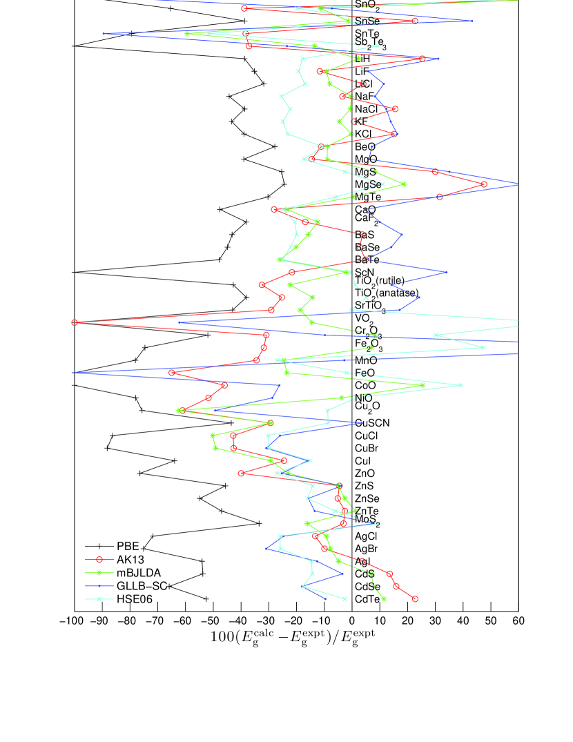
Figure 1: Relative error (in %) with respect to experiment in the fundamental band gap for the set of 76 solids. The values can be found in Refs. Tran and Blaha, 2017; Tran, Ehsan, and Blaha, 2018.

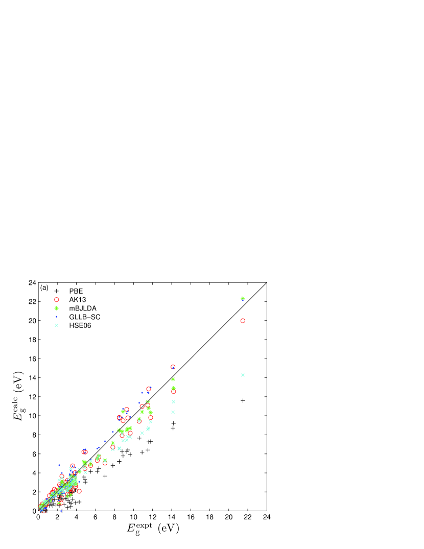
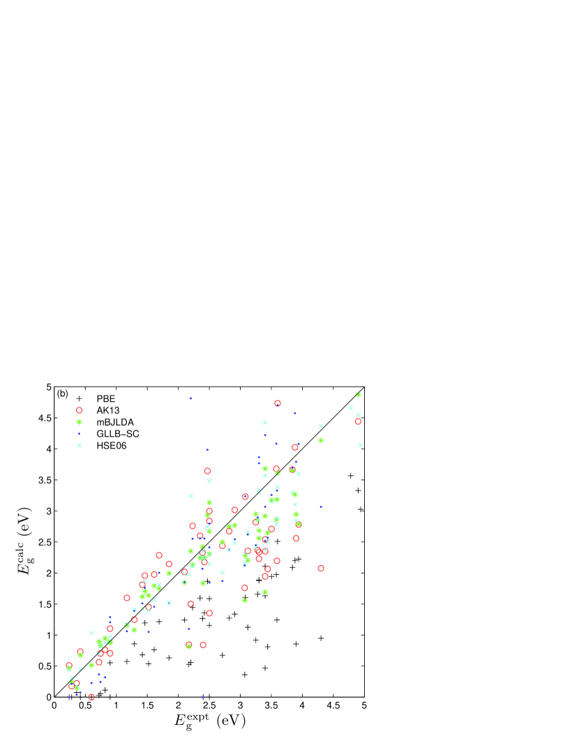
Figure 2: Calculated versus experimental fundamental band gaps for the set of 76 solids. The values can be found in Refs. Tran and Blaha, 2017; Tran, Ehsan, and Blaha, 2018. The lower panel is a zoom of the upper panel focusing on band gaps smaller than 5 eV.

In two of our previous works,Tran and Blaha (2017); Tran, Ehsan, and Blaha (2018) a set of 76 solids was build and used for benchmarking and comparing twelve different DFT methods in total. The tested methods are two LDA-type functionals (LDA and Sloc), four GGAs (PBE, EV93PW91, AK13, and HLE16), two MGGAs (BJLDA and mBJLDA), LB94, GLLB-SC, and two hybrids (HSE06 and B3PW91). The test set (see Fig. 1) consists of a large variety of semiconductors and insulators, most of them being IVA solids, IIIA-VA compounds, transition-metal (TM) chalcogenides/halides, rare gases, or ionic IA-VIIA or IIA-VIA compounds. Among the TM oxides, six of them (Cr₂O₃, Fe₂O₃, MnO, FeO, CoO, and NiO) are AFM with strongly correlated $3d$ electrons. Also included in the set is VO₂ that has been extensively studied (see, e.g, Ref. Zhu and Schwingenschlögl, 2012). Here, the non-magnetic phase of VO₂ is considered. The calculations were done with the WIEN2k all-electron code,Blaha et al. (2018) which is based on the linearized-augmented plane-wave basis set.Singh and Nordström (2006) We mention that the HSE06 results were actually obtained with YS-PBE0,Tran and Blaha (2011) which is also a screened hybrid functional and was shown to lead to basically the same results as HSE06 for the electronic structure.Tran and Blaha (2011) As in Refs. Tran and Blaha, 2017; Tran, Ehsan, and Blaha, 2018, we have decided to use the acronym HSE06.

The mean errors with respect to experiment Crowley, Tahir-Kheli, and Goddard (2016); Lucero, Henderson, and Scuseria (2012); Bernstorff and Saile (1986); Gillen and Robertson (2013); Schimka, Harl, and Kresse (2011); Koller, Blaha, and Tran (2013); Skone, Govoni, and Galli (2014); Shi, Eglitis, and Borstel (2005); Lee et al. (2016); Ganose and Scanlon (2016); Groh et al. (2009) are reported in Table 1, where M(R)E and MA(R)E denote the mean (relative) and mean absolute (relative) error, respectively. Here, we summarize only the most important observations from Refs. Tran and Blaha, 2017; Tran, Ehsan, and Blaha, 2018. With a MAE around 2 eV, the most inaccurate xc methods are LDA, PBE, and LB94. EV93PW91 and BJLDA are only slightly better with $\text{MAE}\sim 1.5$ eV. For the more accurate methods, the ranking depends on whether the MAE or the MARE is considered, however for both quantities mBJLDA is the most accurate method with $\text{MAE}=0.47$ eV and $\text{MARE}=15$%. The hybrid HSE06 has also a very low MARE (17%), while GLLB-SC is the second most accurate method in terms of MAE (0.64 eV).

The detailed results for the 76 solids are shown graphically on Figs. 1 and 2 for selected methods. As LDA, PBE systematically underestimates the band gap and this is particularly severe for small band gaps. mBJLDA does not show a pronounced trend towards underestimation or overestimation, such that the ME and MRE are among the smallest. However, mBJLDA does not perform well for the Cu¹⁺ compounds (e.g., Cu₂O) and ZnO, but these are basically the only systems for which mBJLDA clearly fails. While GLLB-SC works much better than mBJLDA for the Cu¹⁺ compounds, it strongly underestimates the band gaps in the heavy IIIA-VA semiconductors like InSb by nearly 100%, but also strongly overestimates in a few cases like MgSe and Fe₂O₃. The expensive hybrid HSE06 is very accurate for band gaps smaller than $\sim 7$ eV, but clearly underestimates larger band gaps [see Fig. 2(a)]. Note that mBJLDA, GLLB-SC, and HSE06 underestimate the band gap of ZnO by a similar amount ($\sim 1$ eV).

For the particular case of strongly correlated AFM solids, the mBJLDA results should be considered as excellent and clearly more accurate than all other semilocal methods. Only HSE06 is of similar accuracy. Concerning non-magnetic VO₂, we mention that in Refs. Eyert, 2011; Zhu and Schwingenschlögl, 2012 it is shown that mBJLDA and HSE06 lead to a correct description of the electronic structure of the (insulating) rutile and (metallic) monoclinic phases, while LDA and PBE do not.

III.1.2 Test set of 472 solids

Table 2: Mean errors with respect to experiment for the band gap of 472 solids obtained with various DFT methods. The M(A)E is in eV and the M(A)RE is in %. The results are from Ref. Borlido et al., 2019 and were obtained with the VASP code for all methods, except those for EV93PW91, AK13, and GLLB-SC that were obtained with the WIEN2k code for the present work.

	LDA	PBE	EV93PW91	AK13	HLE16	BJLDA	mBJLDA	SCAN	GLLB-SC	HSE06	PBE0
ME	-1.1	-1.0	-0.7	-0.1	-0.4	-0.7	-0.2	-0.7	0.4	-0.1	0.5
MAE	1.2	1.1	0.8	0.5	0.6	0.8	0.5	0.8	0.7	0.5	0.8
MRE	-47	-41	-22	9	-7	-27	-2	-27	16	10	53
MARE	51	46	36	35	32	36	30	38	39	31	61

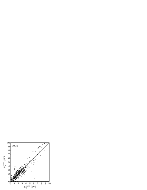
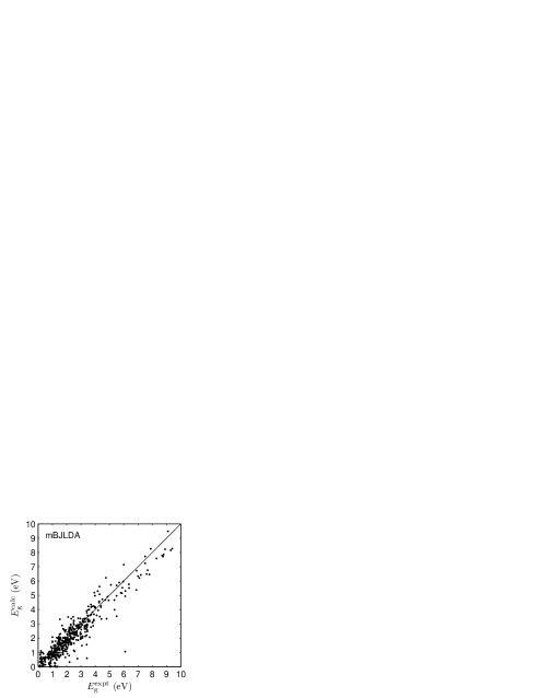
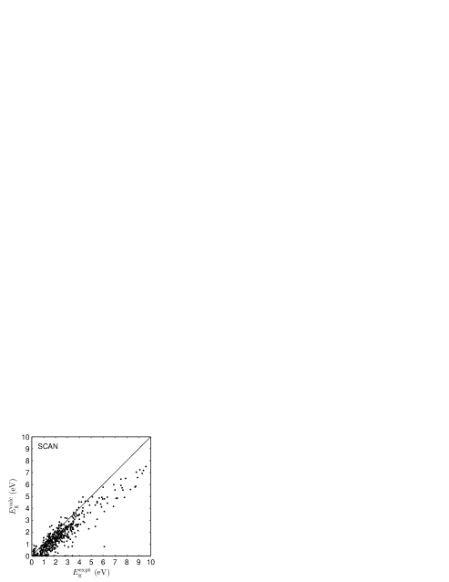
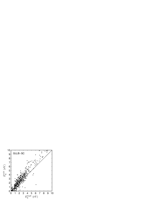
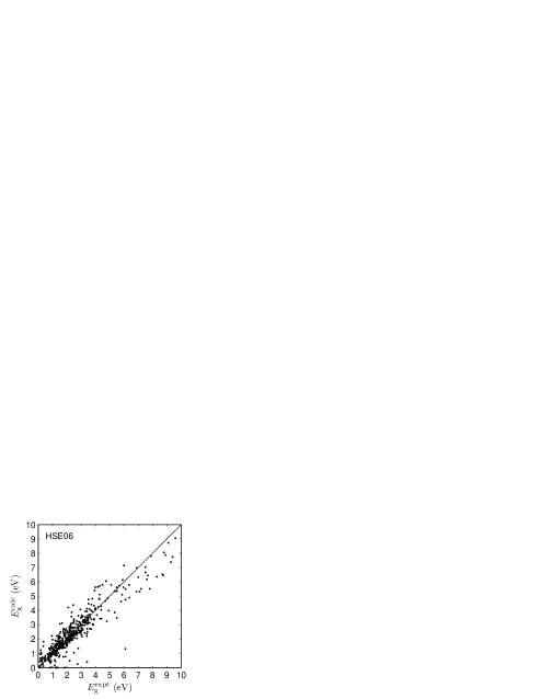
Figure 3: Calculated versus experimental fundamental band gaps smaller than 10 eV for the set of 472 solids.Borlido et al. (2019)

Very recently, a large-scale benchmark study for the band gap was done by some of us.Borlido et al. (2019) The data set consists of 472 solids and, as for the one discussed in the previous section, it consists of a large variety of solids. Nevertheless, this test set contains no strongly correlated AFM TM oxides. The calculations from Ref. Borlido et al., 2019 were done with the VASP code, which uses the projector augmented wave formalism.Blöchl (1994); Kresse and Furthmüller (1996) Additional calculations with the EV93PW91, AK13, and GLLB-SC (and again PBE) methods were performed for the present work using the WIEN2k code. The detailed WIEN2k results are in Table SI of the supplementary material. Here, we mention that the agreement between VASP and WIEN2k band gaps is in general excellent for standard functionals like LDA or PBE. However, for a couple of solids, those with very large band gaps like the rare gases, noticeably larger disagreement can be obtained with other xc methods like mBJLDA or HLE16. In such cases, the discrepancy can be of the order of the eV, which however, has no real impact on the conclusion.

A summary of the statistics for the error is shown in Table 2, and the data for the band gaps smaller than 10 eV are shown in Fig. 3 for selected methods (see Figs. S1-S11 of the supplementary material for all methods and the full range of band gap values). The mBJLDA, AK13, HLE16, and HSE06 methods lead to the lowest MAE and MARE, which are $\sim 0.5$ eV and $30$-$35\%$, respectively. These four methods can be considered as performing equally well. For the test set discussed in Sec. III.1.1, the mBJLDA potential was shown to be clearly more accurate, in particular in terms of MAE. Two reasons may explain why this is not the case for the large test set. First, the errors (in eV, but no in %) with HSE06 are clearly smaller for small band gaps, and since the test set of 472 solids contains (many) more such small band gaps (mainly around 2 eV), it favors HSE06. Regarding AK13 and HLE16, the second reason may be due to the fact that TM oxides, considered in Sec. III.1.1, but not here, are very well described by mBJLDA, but not with AK13 and HLE16.

The other functionals are less accurate. We remark that BJLDA and SCAN lead to quasi-identical mean errors ($\text{MAE}=0.8$ eV and $\text{MARE}=36$-$38$%), and that the screened hybrid HSE06 is much more accurate than the unscreened PBE0. A much more detailed discussion of the results can be found in Ref. Borlido et al., 2019.

III.1.3 Other benchmark studies

Among the xc methods tested for the band gap with the sets of 76 and 472 solids (discussed above), SCAN is the only one consisting of a MGGA energy functional with a potential implemented in the gKS framework. Such MGGA methods are extremely promising for band gap calculation since they are of the semilocal type (and therefore computationally fast) and lead to a non-zero xc derivative discontinuity, allowing for a theoretically justified comparison of the gKS band gap $E_{\text{g}}^{\text{gKS}}$ with the experimental $E_{\text{g}}$.

As discussed above, SCAN is inferior to the semilocal methods that were designed specifically for band gaps (mBJLDA and HLE16) for the set of 472 solids. However, many other MGGA functionals have been proposed, and several of them have been tested for band gaps in Refs. Heyd et al., 2005; Zhao and Truhlar, 2009; Lucero, Henderson, and Scuseria, 2012; Peverati and Truhlar, 2012a, b, c; Xiao et al., 2013; Yang et al., 2016; Verma and Truhlar, 2017b; Wang et al., 2017; Mo, Tian, and Tao, 2017; Jana, Patra, and Samal, 2018; Mejia-Rodriguez and Trickey, 2018; Patra et al., 2019. In most of these studies, the test sets are of smaller size (up to 40 solids) and contain no AFM solids, such that a direct comparison of the mean errors with our two previous benchmarks is not possible. However, it should be possible to get a rough idea of the performance of these MGGAs with respect to mBJLDA or GLLB-SC, which were not considered in these studies.

Truhlar and co-workers have proposed several MGGA functionals that have been tested on band gaps. Among them, an interesting one is HLE17,Verma and Truhlar (2017b) which shows a performance that is similar to the GGA HLE16 and hybrid HSE06.Verma and Truhlar (2017b) For the three functionals, the MAE is 0.30-0.32 eV for a set of 31 semiconductors. For this test set, mBJLDA leads to a MAE of 0.27 eV. However, for the AFM TM monoxides MnO, FeO, CoO, and NiO, HLE17 is clearly worse than HSE06 and mBJLDA by providing band gaps that are too small by 1-2 eV with respect to experiment. Nevertheless, HLE17 is better than SCAN according to the results in Ref. Peng and Perdew, 2017. In Ref. Wang et al., 2017, the MGGA revM06-L was shown to perform better than a certain number of other functionals for the same set of 31 semiconductors. However, the MAE is 0.45 eV, which is larger than HLE17.

To date, HLE17 seems to be the most accurate MGGA (implemented within a gKS framework) according to our knowledge. However, HLE17 is slightly inferior to mBJLDA for the test set of 31 semiconductors and does not perform well for the AFM oxides. Other standard MGGA functionals like TPSSTao et al. (2003) or revTPSS,Perdew et al. (2009) or the recent one from Tao and MoTao and Mo (2016) barely improve over PBE (see, e.g., Ref. Jana, Patra, and Samal, 2018). Also noteworthy is a very recent MGGA functional proposed by Patra et al.Patra et al. (2019) leading to a MAE of 0.69 eV for a set of 67 solids (comprising no AFM TM oxides), which is, however, larger than 0.44 eV obtained with mBJLDA for the same test set.

A short summary of other benchmark studies involving the mBJLDA potential is now given. JiangJiang (2013) compared PBE and mBJLDA on a set of 50 solids, which includes TM dichalcogenides and Ti-containing oxides. As expected mBJLDA is much more accurate than PBE. Another goal of this work was to evaluate the accuracy of the non-self-consistent calculation of the mBJLDA band gap, which consists of one iteration on top of a PBE calculation (mBJLDA@PBE). In most cases, the difference between the mBJLDA and mBJLDA@PBE band gaps is below 0.1 eV. The difference is much larger in rare-gas solids, e.g., Ne where the band gap with mBJLDA@PBE is smaller than the self-consistent one by 4.5 eV. Another case is ZnO where this time the mBJLDA@PBE band gap is larger by $\sim 0.5$ eV. It is also found that mBJLDA@PBE is only slightly less accurate than one-shot $G_{0}W_{0}$ for the TM dichalcogenides.

Lee et al.Lee et al. (2016) calculated the band gap of 270 compounds using PBE, mBJLDA, and $G_{0}W_{0}$. They found experimental values for 32 of these compounds, and for this subset the root mean squared error is 1.77, 0.91, and 0.50 eV for PBE, mBJLDA, and $G_{0}W_{0}$, respectively.

In Ref. Pandey, Kuhar, and Jacobsen, 2017, the performance of the GLLB-SC and mBJLDA potentials were compared on a set consisting of 33 chalcopyrite, kesterite, and wurtzite polymorphs of II-IV-V₂ and III-III-V₂ semiconductors. The GLLB-SC and mBJLDA band gaps are relatively close in the majority of cases. Since the experimental values are known for only half of the systems, a conclusion about the relative accuracy of GLLB-SC and mBJLDA was not really possible.

In a very recent study, Nakano and SakaiNakano and Sakai (2018) calculated the band gap, refractive index, and extinction coefficient of 70 solids with the PBE and mBJLDA methods. In this work, one of the parametrization of mBJLDA from Ref. Koller, Tran, and Blaha, 2012 was used. Similarly as in the test set of 472 solids discussed in Sec. III.1.2, the solids are of various types ranging from simple systems like diamond or BN to more complicated cases like LiTaO₃ or Y₃Al₅O₁₂. For the band gap, the root mean squared error with respect to experiment is 0.44 and 1.69 eV, for mBJLDA and PBE, respectively.

In Ref. Meinert, 2013, Meinert reported PBE and mBJLDA calculations on a set of 26 half-metallic Heusler compounds $X_{2}YZ$, where $X$ and $Y$ are $3d$ TM, and $Z$ is a main group element. One of his conclusions is that mBJLDA gives too large band gaps, while PBE only slightly underestimates. However, as mentioned by Meinert, the experimental measurement of the half-metallic band gap is difficult and can only be made indirectly. In addition, such experimental results were available only for a few of the systems.

On the side of the GLLB-SC potential, we mention Ref. Castelli et al., 2012a, where a MAE of 0.5 eV was obtained for a set of about 30 oxides. GLLB-SC was then further used for the search of new efficient photoelectrochemical cells among several thousands of oxides.Castelli et al. (2012a, b, 2014)

III.1.4 Further discussion

In conclusion, the results published so far have shown that among the computationally fast (i.e., semilocal) methods, the mBJLDA potential is overall the most accurate for band gap prediction. Other methods like the GLLB-SC potential or the MGGA HLE17 may reach similar accuracy for a particular class of systems. Actually, GLLB-SC performs better than mBJLDA for Cu¹⁺ compounds. However, for the AFM TM solids, mBJLDA is clearly superior and reaches the accuracy of the much more expensive hybrid functionals. We mention that the more sophisticated hybrid methods with a fraction $\alpha_{\text{x}}$ of HF exchange that depends on the dielectric function seem to be more accurate than traditional hybrids and mBJLDA.Chen et al. (2018)

We should also mention that Jishi et al.Jishi, Ta, and Sharif (2014) pointed out that, although improving over PBE, mBJLDA still underestimates the band gap in lead halide perovskites by roughly 1 eV when spin-orbit coupling is included in the calculation. They proposed a reparametrization [$\alpha=0.4$ and $\beta=1.0$ bohr^1/2 in Eq. (16)] which leads to excellent agreement with experiment, but would lead to overestimations for other systems (see Sec. V). Similar observations were made in Ref. Traoré et al., 2019 about the more complicated layered hybrid organic-inorganic lead halide perovskites.

Table 3: Fundamental band gap (in eV) in rare-earth oxides (CeO₂ and Ce₂O₃) and one actinide oxide (UO₂). The results were obtained with the WIEN2K code.

	CeO2	Ce2O3	UO2
PBE	2.0	0.0	0.0
HLE16	1.4	0.2	0.0
mBJLDA	2.2	1.3	0.5
GLLB-SC	3.5	1.5	0.9
PBE+$U$	2.5	2.3	2.9
Expt.	3	2.4	2.0

In the literature, not much has been said about the accuracy of specialized potentials like mBJLDA or GLLB-SC for systems with a $4f$ or $5f$ (open) shell at the VBM or CBM. In order to give a vague idea, we considered CeO₂ (non-magnetic), Ce₂O₃ (AFM), and UO₂ (AFM). The results obtained with the WIEN2k code for a few selected methods are shown in Table 3, where in addition to the experimental values, PBE+$U$ results are also given. For all three systems, the PBE+$U$ calculations were done using the fully localized limit versionCzyżyk and Sawatzky (1994) with $U=5$ and $J=0.5$ eV, which are similar to suggested values.Da Silva et al. (2007); He et al. (2013) For CeO₂, mBJLDA (but not HLE16) slightly improves over PBE, while GLLB-SC widens further the band gap. For Ce₂O₃ and UO₂, none of the methods except PBE+$U$ leads to reasonable band gaps. Furthermore, taking into account spin-orbit coupling for UO₂ (not done for the present work) should reduce further the calculated band gap. Overall, GLLB-SC is more accurate than PBE, HLE16, and mBJLDA, but less than PBE+$U$, which should be the preferred fast method for $4f$ and $5f$ systems. Note that the hybrid functional HSE leads to good agreement with experiment for the three systems.Hay et al. (2006); He et al. (2013)

At that point we want to mention other fast DFT schemes for band gap calculations that we did not consider for the present work. A few of them do not consist of a particular xc potential, but of a post-KS-DFT procedure with standard LDA or PBE. The methods of Chan and CederChan and Ceder (2010) and Zheng et al.Zheng et al. (2011) lead to results similar to mBJLDA for typical $sp$-semiconductors, and actually more accurate for ZnO, which is a difficult case for mBJLDA. By making simplifications in the $GW$ equations, Johnson and AshcroftJohnson and Ashcroft (1998) proposed a shift for the conduction band. This is somehow in the same spirit as the GLLB-SC method, but with the disadvantage that the dielectric constant is needed.

III.2 Other properties

In Sec. II.4, it was mentioned that multiplicative potentials like mBJLDA, AK13, or HLE16 leading to band gaps $E_{\text{g}}^{\text{KS}}$ close to $E_{\text{g}}$ may possibly lead to inaccurate results for other properties. Below, a short summary of the performance of xc potentials on properties other than the fundamental band gap is given.

III.2.1 Effective mass and bandwidth

In Refs. Kim et al., 2010; Tran, Ehsan, and Blaha, 2018 (see also Ref. Araujo, de Almeida, and Ferreira da Silva, 2013), the effective hole and electron masses were calculated for five III-V semiconductors (InP, InAs, InSb, GaAs, and GaSb). The results showed that HLE16 and mBJLDA increase very often, but not systematically, the effective masses compared to PBE. With both methods, the tendency is to yield values that are larger than experiment. Overall, the resultsKim et al. (2010); Tran, Ehsan, and Blaha (2018) with HLE16 and mBJLDA are more accurate than with the standard PBE, but less accurate than with the hybrid HSE (as shown recently in Ref. Rödl et al., 2019 for Ge) or EV93PW91. GLLB-SC was shown to be not particularly accurate for the III-V semiconductors.Tran, Ehsan, and Blaha (2018) The overestimation of the effective mass by mBJLDA in various perovskites has been been reported in recent works.Ohkubo and Mori (2017); Traoré et al. (2019) In particular, in Ref. Traoré et al., 2019 a reoptimization of the $\alpha$ and $\beta$ parameters in mBJLDA [Eq. (16)] specific for lead halide perovskites and within a pseudopotential implementation has been proposed (see also Refs. Jishi, Ta, and Sharif, 2014; Jishi, 2016). It is shown that the overestimation of the reduced effective mass with the reoptimized mBJLDA is of similar magnitude as the underestimation with LDA.

As underlined, e.g., in Refs. Singh, 2010a; Smith et al., 2012; Kresse et al., 2012; Waroquiers et al., 2013; Araujo, de Almeida, and Ferreira da Silva, 2013; Traoré et al., 2019; Wang et al., 2019, a narrowing of electronic bands is observed with mBJLDA compared to LDA/PBE, which is related to the increase in the effective mass observed above. On a set of ten cubic semiconductors and insulators, Waroquiers et al.Waroquiers et al. (2013) showed that mBJLDA clearly underestimates the bandwidth with respect to experiment and is less accurate than LDA. For this test set LDA is, on average, as accurate as $G_{0}W_{0}$. Actually, the too narrow bands obtained with mBJLDA have recently been shown to be a source of problem for optical spectra in ZnSe.Wang et al. (2019) A similar reduction in the bandwidth has been observed with the AK13 potentialVlček et al. (2015) and most likely the same problem occurs with HLE16.

In summary, while mBJLDA is much more accurate than the standard LDA and PBE for the fundamental band gap, it seems to be of similar accuracy as (or possibly slightly more accurate than) PBE for the effective mass, but quite inaccurate for the bandwidth.

III.2.2 Optics

The mBJLDA potential has also been used quite frequently for the calculation of the optical properties of solids. A few representative works reporting calculations of (non-)linear optics using the RPA for the dielectric function is given by Refs. Singh, 2010b; Kresse et al., 2012; Karsai et al., 2014; Reshak, 2016; Kopaczek et al., 2016; Ondračka et al., 2017; Ibarra-Hernández et al., 2017; Nakano and Sakai, 2018; Rödl et al., 2019. Without entering into details, a rather general conclusion from all these studies is that mBJLDA improves over LDA and PBE for the optical properties. This is not that surprising since an improvement in the band gap should in principle be followed by a more realistic onset in the absorption spectrum.

We also mention a series of studies from Yabana and co-workers (see, e.g., Refs. Wachter et al., 2014; Sato et al., 2015a, b; Wachter et al., 2015; Uemoto et al., 2019; Yamada and Yabana, 2019) who used mBJLDA within time-dependent DFT (TDDFT) to study nonlinear effects induced by strong short laser pulses. For instance, in Ref. Sato et al., 2015b they showed that in Si and Ge, mBJLDA and HSE lead to very similar results (for the dielectric function and excitation energies) and improve over LDA. However, it was also noticed that special care is needed in order to get a stable time evolution in TDDFT when using the mBJLDA potential.Sato et al. (2015b) Similar problems with the original BJ potential were reported in Ref. Karolewski, Armiento, and Kümmel, 2013.

Regarding other xc methods, Vlček et al.Vlček et al. (2015) reported an improvement (with respect to PBE) in the dielectric constant when using AK13. Calculations of the dielectric constant with TDDFTYan, Jacobsen, and Thygesen (2012) showed that GLLB-SC degrades the results with respect to LDA, in particular if the derivative discontinuity is taken into account. However, these errors obtained with GLLB-SC were attributed to the missing electron-hole interaction in the calculation of the RPA (or adiabatic LDA) response function.

III.2.3 Magnetism

Table 4: Atomic spin magnetic moment $\mu_{S}$ (in $\mu_{\text{B}}$) of AFM TM oxides compared to the experimental total moment $\mu_{S}+\mu_{L}$. The orbital moment $\mu_{L}$ should be in the range 0.6-1 $\mu_{\text{B}}$ for FeO, Svane and Gunnarsson (1990); Tran et al. (2006); Radwanski and Ropka (2008); Schrön and Bechstedt (2013) 1-1.6 $\mu_{\text{B}}$ for CoO, Svane and Gunnarsson (1990); Solovyev, Liechtenstein, and Terakura (1998); Shishidou and Jo (1998); Neubeck et al. (2001); Jauch and Reehuis (2002); Ghiringhelli et al. (2002); Radwanski and Ropka (2004); Tran et al. (2006); Radwanski and Ropka (2008); Boussendel et al. (2010); Schrön and Bechstedt (2013) 0.3-0.45 $\mu_{\text{B}}$ for NiO, Svane and Gunnarsson (1990); Fernandez et al. (1998); Neubeck et al. (2001); Radwanski and Ropka (2004, 2008) and smaller for the other cases. The theoretical results, obtained with the WIEN2k code, are from Ref. Tran, Ehsan, and Blaha, 2018.

Method	MnO	FeO	CoO	NiO	CuO	Cr2O3	Fe2O3
PBE	4.17	3.39	2.43	1.38	0.38	2.44	3.53
HLE16	4.51	3.62	2.59	1.48	0.40	2.96	4.02
mBJLDA	4.41	3.58	2.71	1.75	0.74	2.60	4.09
GLLB-SC	4.56	3.74	2.73	1.65	0.55	2.99	4.43
HSE06	4.36	3.55	2.65	1.68	0.67	2.61	4.08
Expt.	4.58	3.32,4.2,4.6	3.35,3.8,3.98	1.9,2.2	0.65	2.44,2.48,2.76	4.17,4.22

Concerning magnetism, it has been shown that the mBJLDA potential provides very accurate values of the atomic magnetic moment in AFM systems with localized electrons. In Refs. Tran and Blaha, 2009; Koller, Tran, and Blaha, 2011; Botana et al., 2012; Tran, Ehsan, and Blaha, 2018, we showed that mBJLDA increases by 0.2-0.4 $\mu_{\text{B}}$ the atomic spin moment $\mu_{S}$ with respect to PBE. Since PBE quasi-systematically underestimates $\mu_{S}$ in AFM systems, such an increase leads to better agreement with experiment. In Table 4, results from Ref. Tran, Ehsan, and Blaha, 2018 for AFM TM oxides are reproduced for selected xc methods. Compared to PBE, all other methods lead to larger $\mu_{S}$ values. Since there is sometimes a rather large uncertainty in the experimental value and, furthermore, the orbital component $\mu_{L}$ is not known precisely, it is difficult to say which method is the best. Anyway, in most cases the agreement with experiment is much improved compared to PBE and satisfactory. We just note that HLE16 seems to underestimate (overestimate) the value in CuO (Cr₂O₃) and that GLLB-SC overestimates for Cr₂O₃ and Fe₂O₃. The advantage of these methods over DFT+$U$,Anisimov, Zaanen, and Andersen (1991) which is widely used for AFM oxides, is that they do not contain a system-dependent parameter like $U$.

Table 5: Unit cell spin magnetic moment $\mu_{S}$ (in $\mu_{\text{B}}$/atom) of $3d$ TM. The experimental values are also spin magnetic moments. The theoretical results, obtained with the WIEN2k code, are from Ref. Tran, Ehsan, and Blaha, 2018.

Method	Fe	Co	Ni
PBE	2.22	1.62	0.64
HLE16	2.72	1.72	0.63
mBJLDA	2.51	1.69	0.73
GLLB-SC	3.08	1.98	0.81
HSE06	2.79	1.90	0.88
Expt.	1.98,2.05,2.08	1.52,1.58,1.55-1.62	0.52,0.55

Table 5 shows the results for $\mu_{S}$ in the ferromagnetic metals Fe, Co, and Ni (results from Ref. Tran, Ehsan, and Blaha, 2018). Unlike in AFM systems with localized electrons, the LDA and standard GGAs lead usually to reasonable values of the moment in itinerant metals. Indeed, PBE only slightly overestimates with respect to experiment, while the other methods clearly overestimate the values. For the three metals, GLLB-SC and HSE06 overestimate more than mBJLDA and HLE16. We mention that the reverse has been observed by SinghSingh (2010a) in the ferromagnetic metal Gd, a $4f$-system, in which the mBJLDA moment is smaller than the PBE one and than the experimental value by $\sim 1$ $\mu_{\text{B}}$. Thus, contrary to what has been observed in $3d$ magnetic systems, the mBJLDA potential reduces the exchange splitting in Gd (due to an increase of occupancy of the minority $4f$ states) and shifts the $spd$-bands up with respect to the $4f$ bands.

In the work of MeinertMeinert (2013) on half-metallic Heusler compounds already mentioned in Sec. III.1.3, it is shown that the PBE and mBJLDA magnetic moments are the same in most cases, which is simply due to the half-metallic state. Only for Co₂FeSi and Co₂FeGe the moment is clearly different with mBJLDA (larger by $\sim 0.35$ $\mu_{\text{B}}$) and actually in better agreement with experiment.

Regarding the performance of MGGA functionals implemented with a non-multiplicative potential, a certain number of results are available for ferromagnetic metals. Sun et al. (2011); Isaacs and Wolverton (2018); Jana, Patra, and Samal (2018); Romero and Verstraete (2018); Ekholm et al. (2018); Fu and Singh (2018a, 2019); Mejía-Rodríguez and Trickey (2019) From these studies the most interesting results concern the SCAN functional, which has been shown to overestimate the magnetic moment, and sometimes by a rather large amount (e.g., $\sim 0.5$ $\mu_{\text{B}}$ for Fe). However, such overestimation is not systematically observed with functionals of this class, since other MGGA functionals like TPSSTao et al. (2003) or revTPSSPerdew et al. (2009) lead to values similar to PBE.Sun et al. (2011); Jana, Patra, and Samal (2018); Fu and Singh (2019)

In summary, the standard LDA and GGA lead to magnetic moments which are qualitatively correct for itinerant metals, but not for AFM solids with strongly correlated electrons (strong underestimation). On the other hand, methods giving much more reasonable magnetic moments in AFM solids, e.g., mBJLDA, GLLB-SC, or HSE06, lead to strong overestimation in itinerant metals. However, it is important to note that the overestimation of the moment in Fe, Co, and Ni with mBJLDA is much less severe than with GLLB-SC and HSE06 (an explanation is provided in Sec. V). Note that the inadequacy of hybrid functionals for metals has been documented.Paier et al. (2006); Tran, Koller, and Blaha (2012); Jang and Yu (2012); Gao et al. (2016b) Currently, there is no DFT method that is able to provide qualitatively correct values of the moment in itinerant metals and AFM solids simultaneously.

III.2.4 Electron density

The quality of the electron density $\rho$ can be measured by considering the electric field gradient (EFG) or the X-ray structure factors. The EFG is defined as the second derivative of the Coulomb potential at a nucleus and, therefore, depends on the charge distribution in the solid. In Ref. Tran, Ehsan, and Blaha, 2018, the calculated EFG of seven metals (Ti, Zn, Zr, Tc, Ru, Cd, and Cu₂Mg) and two non-metals (CuO and Cu₂O) has been calculated and compared to experiment. For some of the systems, the error bar on the experimental value is quite large, nevertheless it was possible to draw some conclusions on the accuracy of the methods. The method that is the most accurate overall is the GLLB-SC potential that leads to reasonable errors for all systems. The methods that were shown to be quite inaccurate are LDA, Sloc, HLE16, mBJLDA, and LB94.

In the same work,Tran, Ehsan, and Blaha (2018) the calculated and experimental X-ray structure factors of Si were compared. The best method is the screened hybrid HSE06, followed by PBE, EV93PW91, and BJLDA. The mBJLDA potential is less accurate than these methods, but slightly more accurate than LDA. The Sloc and HLE16 were shown to be much more inaccurate than all other methods, while LB94 and GLLB-SC are also very inaccurate, but to a lesser extent. Actually, in the case of GLLB-SC it is the core density that is particularly badly described, while the valence density seems to be rather accurate (see Ref. Tran, Ehsan, and Blaha, 2018 for details), which is consistent with the very good description of the EFG mentioned above.

In an interesting recent study,Medvedev et al. (2017) it was shown that functionals like SCAN or HSE06 which were constructed more from first-principles by using mathematical constraints rather than empirically by fitting a large number of coefficients produce more accurate electron density, however the test set consists only of atoms/cations with 2, 4, or 10 electrons. Highly parametrized functionals like those of the Minnesota familyZhao and Truhlar (2008) are much less accurate.

To finish this section, we mention a study on VO₂, where various functionals are compared for the electron density. Accurate electron densities from Monte-Carlo calculations were used as reference. It is shown that hybrid functionals like HSE are more accurate than LDA and PBE.

IV Summary

From the overview of the literature results presented in Sec. III, the main conclusions are the following:

• Among the semilocal methods, the mBJLDA potential is on average the most accurate for the fundamental band gap. Furthermore, mBJLDA is at least as accurate as hybrid functionals like HSE06. Only the most advanced methods, namely the dielectric-function-dependent hybrid functionals and $GW$, can be consistently more accurate than mBJLDA.

• A particularly strong advantage of mBJLDA over the other methods is its reliability for all kinds of systems. mBJLDA is more or less equally accurate for large band gap insulators (ionic solids, rare gases), $sp$-semiconductors, and systems with TM atoms including AFM systems with localized $3d$-electrons.

• All other semilocal potentials are very unreliable for the band gap in AFM systems.

• The cases where mBJLDA is clearly not accurate enough are the Cu¹⁺ compounds (for which GLLB-SC works much better), but also ZnO, where the band gap is still underestimated by at least 1 eV. Note that a modification of mBJLDA, called the universal correction,Räsänen, Pittalis, and Proetto (2010) may help for Cu¹⁺ compounds (see Ref. Tran et al., 2015 for details). Lead halide perovskites require another set of parameters $\alpha$ and $\beta$ in mBJLDA, while none of the multiplicative potentials leads to meaningful band gaps for the $4f$ and $5f$ systems.

• The bandwidth is not reproduced accurately by mBJLDA which makes the bands too narrow. LDA and PBE are more accurate than mBJLDA.

• The magnetism in AFM systems is very well described with mBJLDA and as accurately as with hybrid functionals. In ferromagnetic metals the magnetic moment is too large, however the overestimation is not as large as with GLLB-SC and hybrid functionals.

• The electron density does not seem to be particularly well described by mBJLDA. The standard PBE is more accurate, while HLE16 and GLLB-SC are extremely inaccurate. HSE06 is particularly good for the electron density of Si.

• Beside mBJLDA, DFT+$U$ is the only other computationally cheap method that is able to provide qualitatively correct results in AFM systems for the band gap and magnetic moment.

Thus, this summary shows that the mBJLDA potential is currently the best alternative to the much more expensive hybrid or $GW$ methods. This explains why it has been implemented in various codes Kim et al. (2010); César et al. (2011); Marques, Oliveira, and Burnus (2012); Germaneau, Su, and Zheng (2013); Meinert (2013); Ye (2015); Traoré et al. (2019); Bartók and Yates (2019); Smidstrup et al. (2019) and used for numerous applications. Examples are the search for efficient thermoelectric materials, Parker and Singh (2012); Parker, Chen, and Singh (2013); Pardo, Botana, and Baldomir (2013); Shi et al. (2015); Zhang et al. (2016); Xing et al. (2017); Kang and Kotliar (2018); Liu et al. (2018); He et al. (2018); Fu and Singh (2018b); Zhu et al. (2018, 2019); Matsumoto et al. (2019); Terashima et al. (2019) topological insulators, Feng et al. (2010, 2011, 2012); Zhu, Cheng, and Schwingenschlögl (2012); Agapito et al. (2013); Sheng et al. (2014); Küfner and Bechstedt (2015); Shi et al. (2015); Li et al. (2015); Arnold et al. (2016a); Kang et al. (2016); Brydon et al. (2016); Ruan et al. (2016); Cao et al. (2017); Rong et al. (2017); Arnold et al. (2016b); Quan, Yin, and Pickett (2017); Oinuma et al. (2017); Zhang et al. (2017); Kim et al. (2018); Parveen et al. (2018); Tang et al. (2019) or materials for photovoltaics. Li and Singh (2017); Zhang et al. (2018); Li and Singh (2019); Ong et al. (2019) The mBJLDA potential has also been used for the screening of materials or in relation to machine learning techniques Lee et al. (2016); Choudhary et al. (2018, 2019) (see Refs. Castelli et al., 2012a, b, 2014; Miró, Audiffred, and Heine, 2014; Rasmussen and Thygesen, 2015; Park et al., 2019 for such works using the GLLB-SC potential). Furthermore, it has been shown to be accurate for the calculation of the ELNES (energy loss near-edge structure) spectrum of NiO,Hetaba et al. (2012) and used recently for the band gap calculation of configurationally disordered semiconductors.Xu and Jiang (2019) Nevertheless, as a technical detail we should mention that the number of iterations to achieve self-consistent field convergence is usually (much) larger with the mBJLDA potential than with other potentials.

V Outlook

The question is why mBJLDA is more accurate than all other semilocal methods. The main reason is the use of two ingredients: the kinetic-energy density $t_{\sigma}$ and the average of $\nabla\rho/\rho$ in the unit cell $g$ [Eq. (17)], that are now discussed.

As illustrated and discussed in previous works,Tran, Blaha, and Schwarz (2007); Tran and Blaha (2017); Tran, Ehsan, and Blaha (2018) the mBJLDA potential is, compared to the PBE potential, more negative around the nuclei (where the orbital of the VBM is usually located) and less negative in the interstitial region (where the orbital of the CBM is located). This enlarges the band gap. This mechanism, which works in most ionic solids and typical $sp$-semiconductors, is also used by the GGAs AK13, HLE16, and Sloc. However, these GGAs are not accurate for AFM systems, where the band gap may have a strong onsite $d$-$d$ character. In Ref. Koller, Tran, and Blaha, 2011 it is shown that the second term in Eq. (15), which is proportional to $\sqrt{t_{\sigma}/\rho_{\sigma}}$, allows the potential to act differently on orbitals with different angular distributions (e.g., $t_{2g}$ versus $e_{g}$ of the $3d$ states) and increase a $d$-$d$ band gap. In order to do this, such a term in the mBJLDA potential is much more efficient than what GGA potentials can do. Actually, the $t_{\sigma}$-dependency in mBJLDA is strong, and most likely much stronger than in any other MGGA like SCAN or HLE17, which are not as good as mBJLDA for AFM solids.

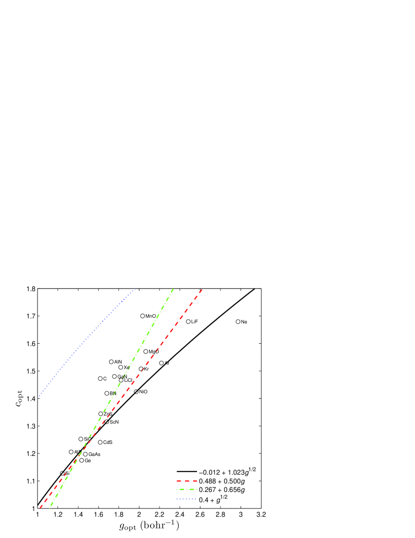
Figure 4: Plot of $c_{\text{opt}}$ versus $g_{\text{opt}}$ (see text for explanations). The fit of these data pointsTran and Blaha (2009) given by Eq. (16) is represented by the solid curve. The two fits (of different sets of solids) proposed in Ref. Koller, Tran, and Blaha, 2012 are represented by the dashed and dashed-dotted curves, and the fit from Ref. Jishi, Ta, and Sharif, 2014 specific for lead halide perovskites is represented by the dotted curve.

Table 6: Results obtained from mBJLDA calculations. Value of $g=g_{\text{SC}}$ [Eq. (17)] (in bohr^-1) obtained at the end of a usual self-consistent (SC) calculation. Fundamental band gap (in eV) and spin magnetic moment $\mu_{S}$ (in $\mu_{\text{B}}$) obtained from a usual calculation ($g=g_{\text{SC}}$) or with $g$ fixed ($g=g_{\text{fixed}}$) to the value obtained for the corresponding AFM oxide (for a metal) or metal (for a AFM oxide). The spin magnetic moment is the value in the unit cell and per atom for metals and inside the TM atomic sphere for the AFM oxides.

	Fe	Co	Ni	Cu	FeO	CoO	NiO	CuO
$g_{\text{SC}}$
	1.40	1.48	1.54	1.52	1.92	1.95	1.97	1.93
Fundamental band gap
With $g=g_{\text{SC}}$	0	0	0	0	1.84	3.14	4.14	2.27
With $g=g_{\text{fixed}}$	0	0	0	0	1.06	1.99	3.09	1.54
$\mu_{S}$
With $g=g_{\text{SC}}$	2.51	3.38	0.73	0	3.58	2.71	1.75	0.74
With $g=g_{\text{fixed}}$	2.53	3.43	0.80	0	3.49	2.63	1.67	0.67

The integral given by Eq. (17), $g$, is even more crucial in explaining the success of the mBJLDA potential. Figure 4 shows a plot of $c_{\text{opt}}$ versus $g_{\text{opt}}$, where $c_{\text{opt}}$ is the value of $c$ in Eq. (16) that would exactly lead to the experimental band gap and $g_{\text{opt}}$ is the value of $g$ obtained at the end of the self-consistent mBJLDA calculation done with $c_{\text{opt}}$. This is shown for all the solids, except two (FeO and ZnO), that were considered in our original work.Tran and Blaha (2009) A correlation between $c_{\text{opt}}$ and $g_{\text{opt}}$ is clearly visible and the fit of these data that we chose in Ref. Tran and Blaha, 2009 is given by Eq. (16) with $\alpha=-0.012$ and $\beta=1.023$ bohr^1/2. Alternative fitsKoller, Tran, and Blaha (2012) that were determined by using different sets of solids, e.g., focusing on small band gaps are also shown. This rather clear correlation between $c_{\text{opt}}$ and $g_{\text{opt}}$ allows for a meaningful fit $c(g)$, which, when used in the mBJLDA potential, produces accurate band gaps. However, as mentioned in Sec. III, the standard parametrization of $c$ is not good enough for lead halide perovskites, which require other values of $\alpha$ and $\beta$, and as shown in Fig. 4 this parametrization would lead to an overestimation of the band gap for other solids (in general, the band gap increases in a monotonous way with respect to $c$). Another illustration of the importance of $g$ is given in Table 6, where the value of $g$ for itinerant $3d$ TM and their oxides is shown. There is a clear difference between the metals and the oxides. While the value of $g$ is in the range 1.40$-$1.54 bohr^-1 for the metals, it is much larger, 1.92$-$1.97 bohr^-1, for the monoxides. From a more detailed analysis, we could see that this difference comes more particularly from the interstitial region, which is on average more inhomogeneous (larger $\left|\nabla\rho\right|/\rho$) for the oxides. However, also around the TM atom $\left|\nabla\rho\right|/\rho$ is larger for the oxides, which therefore also contributes in making $g$ larger compared to the metal. If the calculation for the TM oxides is done by fixing the value of $g$ in Eq. (16) to the value of the corresponding metal, then a large decrease of 0.7$-$1.1 eV in the band gap (and a large discrepancy with experiment) is obtained (Table 6). The same is observed for the magnetic moment, which is reduced in the oxides when the $g$ of the metal is used. Conversely, using the value of $g$ from the oxide for the calculation on the metals leads to an increase of the magnetic moment. The important point to note is that, in any case, using the incorrect $g$ (i.e., the one from the other system) leads to much larger errors. We mention that other works using an average in the unit cell involving the density can be found in Refs. Clark and Robertson, 2010; Marques et al., 2011; Borlido, Marques, and Botti, 2018; Terentjev, Constantin, and Pitarke, 2018; Wang and Jiang, 2019.

However, since the mBJLDA potential is certainly not providing an optimal band gap in every case, and the results for other properties like the bandwidth or the electron density are even worse than with the standard PBE, there is room for improvement. As already mentioned in this work, forcing a multiplicative potential to give KS band gaps $E_{\text{g}}^{\text{KS}}$ close to the experimental $E_{\text{g}}$ is not really correct from the formal point of view and may result in a potential that is inappropriate for other properties. A derivative discontinuity $\Delta_{\text{xc}}$ should be present somewhere in the theory. $\Delta_{\text{xc}}$ is included in the gKS band gap $E_{\text{g}}^{\text{gKS}}$ with non-multiplicative potentials (MGGA and hybrid) or obtained from a post-KS calculation with the GLLB-SC potential.

Thus, from the discussion above, the strategy to follow for the construction of a computationally fast and generally accurate xc potential that alleviates the problems encountered with mBJLDA is quite obvious:

• The potential should be based on one of these two types: non-multiplicative MGGA or multiplicative of the GLLB-SC type. Then, a derivative discontinuity is available as it should be.

• Since both $t_{\sigma}$ and $g$ were shown to be crucial for the mBJLDA potential, most likely they can be useful for other types of potentials (by definition $t_{\sigma}$ is used in a MGGA). Note that instead of $g$, a variant may be used, i.e., the average in the unit cell of a quantity different from $\nabla\rho/\rho$ may be more useful.

However, we mention that attempts (presented in Ref. Tran, Ehsan, and Blaha, 2018 or unpublished) to improve over the GLLB-SC potential along these lines have been unsuccessful up to now. For instance, one of the most sophisticated variants of Eq. (LABEL:eq:vxcGLLBSC) that we have considered is of the form (the formula for $\Delta_{\text{x}}$ should be modified accordingly)

$$v_{\text{xc},\sigma}(\mathbf{r}) = cv_{\text{x},\sigma}^{\text{BR}}(\mathbf{r})+\left(3c-2\right)F_{\sigma}(\mathbf{r})K_{\text{x}}^{\text{LDA}}$$

$$\times\sum_{n,\mathbf{k}}w_{n\mathbf{k}\sigma}\sqrt{\epsilon_{\text{H}}-\epsilon_{n\mathbf{k}\sigma}}\frac{\left|\psi_{n\mathbf{k}\sigma}(\mathbf{r})\right|^{2}}{\rho_{\sigma}(\mathbf{r})}+v_{\text{c},\sigma}^{\text{PBEsol}}(\mathbf{r}),$$

where $F_{\sigma}$ is a function that depends and $\rho_{\sigma}$, $\nabla\rho_{\sigma}$, and $t_{\sigma}$ and should satisfy $F_{\sigma}=1$ for a constant electron density in order to recover the homogeneous electron gas limit, and $c$ is a function that depends on some average in the unit cell similar to Eq. (16). With Eq. (LABEL:eq:vxcGLLBvar), that is of course inspired by the mBJLDA potential [Eq. (15)], we have not been able to find a strategy to parametrize $c$ such that a clear correlation like in Fig. 4 for mBJLDA is obtained.

There are also a few drawbacks or challenges that should be mentioned:

• Modelizing a potential directly without requiring that it is a functional derivative is much easier and leads to much more flexibility. However, such stray potentials lead to problemsGaiduk and Staroverov (2009); Gaiduk, Chulkov, and Staroverov (2009); Karolewski, Armiento, and Kümmel (2013) and do not allow total-energy calculations. Thus, having a potential that is the derivative of a functional $E_{\text{xc}}$ would be certainly much more interesting, but also much more challenging. AK13 and HLE16 satisfy this requirement, but the energy $E_{\text{xc}}$ is very inaccurate.Cerqueira, Oliveira, and Marques (2014); Lindmaa and Armiento (2016); Verma and Truhlar (2017a)

• The use of the average in the unit cell of some quantity, e.g. $g$ [Eq. (17)], works only in the case of bulk solids. Calculating such averages for systems with vacuum (surface or molecule) or interfaces makes no sense. Possible solutions to this problem have been proposed in Refs. Marques et al., 2011; Borlido, Marques, and Botti, 2018 and consist of taking the average not over the unit cell, but over a region localized around the position $\mathbf{r}$ where the potential is calculated. However, it is not clear how far such region should extend to bring enough nonlocal information.

• The use of the highest occupied and lowest unoccupied orbital energies like in the GLLB-SC potential [Eqs. (LABEL:eq:vxcGLLBSC) and (19)] is also problematic. For instance, the values of $\epsilon_{\text{H}}$ and $\epsilon_{\text{L}}$ for an interface correspond to one of the two bulk solids, while they correspond to the respective bulk solids when they are treated separately. This is somehow inconsistent. The solution would be to define position-dependent functions replacing $\epsilon_{\text{H}}$ and $\epsilon_{\text{L}}$.

Trying to overcome these problems makes the search of a generally applicable xc potential even more difficult, however, as a first step they can be ignored.

Supplementary Material

See supplementary material for the detailed results for the band gap of the 472 solids discussed in Sec. III.1.2.