Sparsity Emerges Naturally in Neural Language Models

Abstract

Concerns about interpretability, computational resources, and principled inductive priors have motivated efforts to engineer sparse neural models for NLP tasks. If sparsity is important for NLP, might well-trained neural models naturally become roughly sparse? Using the Taxi-Euclidean norm to measure sparsity, we find that frequent input words are associated with concentrated or sparse activations, while frequent target words are associated with dispersed activations but concentrated gradients. We find that gradients associated with function words are more concentrated than the gradients of content words, even controlling for word frequency.

1 Introduction

Researchers in NLP have long relied on engineering features to reflect the sparse structures underlying language. Modern deep learning methods promised to relegate this practice to history, but have not eliminated the interest in sparse modeling for NLP. Along with concerns about computational resources Chen et al. (2016); Narang et al. (2017b) and interpretability Murphy et al. (2012); Subramanian et al. (2018), human intuitions continue to motivate sparse representations of language. For example, some work applies assumptions of sparsity to model latent hard categories such as syntactic dependencies Padó and Lapata (2007) or phonemes Cotterell and Eisner (2018). Niculae and Blondel (2017) found that a sparse attention mechanism outperformed dense methods on some NLP tasks; Narang et al. (2017a) found sparsified versions of LMs that outperform dense originals. Attempts to engineer sparsity rest on an unstated assumption that it doesn’t arise naturally when neural models are learned. Is this true?

Using a simple measure of sparsity, we analyze how it arises in different layers of a neural language model in relation to word frequency. We show that the sparsity of a word representation increases with exposure to that word during training. We also find evidence of syntactic learning: gradient updates in backpropagation depend on whether a word’s part of speech is open or closed class, even controlling for word frequency.

2 Methods

Language model.

Our LM is trained on a corpus of tokenized, lowercased English Wikipedia (70/10/20 train/dev/test split). To reduce the number of unique words (mostly names) in the corpus, we excluded any sentence with a word which appears fewer than 100 times. Those words which still appear fewer than 100 times after this filter are replaced with <UNK>. The resulting training set is over 227 million tokens of around 19.5K types.

Figure 1: LM architecture for target word distribution $\hat{x}_{t}$, showing gradient updates from observed word $x_{t}$.

We use a standard 2-layer LSTM LM trained with cross entropy loss for 50 epochs. The pipeline from input $x_{t-1}$ at time step $t-1$ to predicted output distribution $\hat{x}$ for time $t$ is described in Figure 1, illustrating intermediate activations $h_{t}^{e}$, $h_{t}^{1}$, and $h_{t}^{2}$. At training time, the network observes $x_{t}$ and backpropagates the gradient updates $\bar{h}_{t}^{e}$, $\bar{h}_{t}^{1}$, $\bar{h}_{t}^{2}$, and $\bar{x}_{t}$.

The embeddings produced by the encoding layer are 200 units, and the recurrent layers have 200 hidden units each. The batch size is set to forty, the maximum sequence length to 35, and the dropout ratio to 0.2. The optimizer is standard SGD with clipped gradients at $\ell_{2}=0.25$, where the learning rate begins at 20 and is quartered whenever loss fails to improve.

Measuring sparsity.

We measure the sparsity of a vector $v$ using the reciprocal of the Taxicab-Euclidean norm ratio (Repetti et al., 2015). This measurement has a long history as a measurement of sparsity in natural settings (Zibulevsky and Pearlmutter, 2001; Hoyer, 2004; Pham et al., 2017; Yin et al., 2014) and is formally defined as $\chi(v)=\|v\|_{2}/\|v\|_{1}$. The relationship between

sparsity and this ratio is illustrated in two dimensions in the image on the right, in which darker blue regions are more concentrated. The pink circle shows the area where $\ell_{2}\leq 1$ while the yellow diamond depicts $\ell_{1}\leq 1$. For sparse vectors $\langle 1,0\rangle$ or $\langle 0,1\rangle$, the norms are identical so $\chi$ is 1, its maximum. For a uniform vector like $\langle 1,1\rangle$, $\chi$ is at its smallest. In general, $\chi(v)$ is higher when most elements of $v$ are close to 0; and lower when the elements are all similar in value.

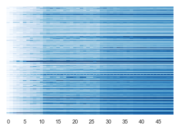
Figure 2: Average sparsity $\chi(\bar{h_{t}^{2}})$ over all training epochs (x-axis), for target words $x_{t}$ occurring more than 100k times in training. Target words are sorted from most frequent (bottom) to least frequent (top).

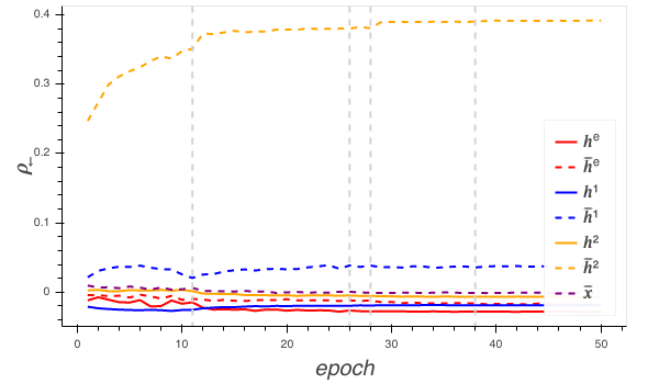
(a) $\rho_{\leftarrow}$ correlation with target word frequency

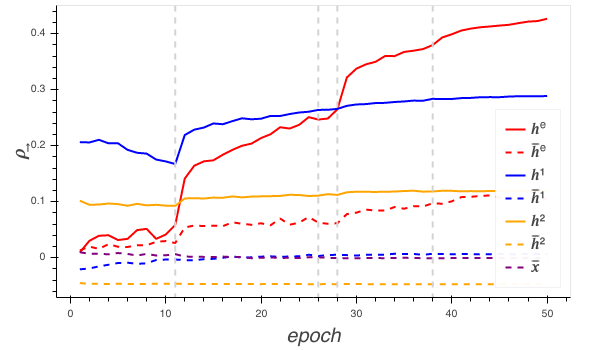
(b) $\rho_{\rightarrow}$ correlation with input word frequency

Figure 3: Correlation between mean sparsity of a word’s representation and word frequency. Vertical dashed lines indicate when the optimizer has rescaled the step size.

3 Experiments

Sparsity is closely related to the behavior of a model: If only a few units hold most of the mass of a representation, the activation vector will be highly concentrated. If a neural network relies heavily on a small number of units in determining its predictions, the gradient will be highly concentrated. A highly concentrated gradient is mainly modifying a few specific pathways. For example, it might modify a neuron associated with particular inputs like parentheses Karpathy et al. (2015), or properties like sentiment Radford et al. (2017).

Representations of Target Words.

Our first experiments look at the relationship of sparsity to target word $x_{t}$. Gradient updates triggered by the target are often used to identify units that are relevant to a prediction (Li et al., 2015), and as shown in Figure 2, gradient sparsity increases with both the frequency of a word in the corpus and the overall training time. In other words, more exposure leads to sparser relevance. Because the sparsity of $\bar{h}^{2}$ increases with target word frequency, we measure not sparsity itself but the Pearson correlation, over all words $w$, between word frequency and mean $\chi(h)$ over representations $h$ where $w$ is the target:

$$\rho_{\leftarrow}(h)=\textrm{corr}_{w}(\mu_{t:x_{t}=w}(\chi(h_{t})),\textrm{freq}(w))$$

Here (Figure 3(a)) we confirm that concentrated gradients are not a result of concentrated activations, as activation sparsity $\chi(h^{2})$ is not correlated with target word frequency.

The correlation is strong and increasing only for $\rho_{\leftarrow}(\bar{h}^{2})$. The sparse structure being applied is therefore particular to the gradient passed from the softmax to the top LSTM layer, related to how a word interacts with its context.

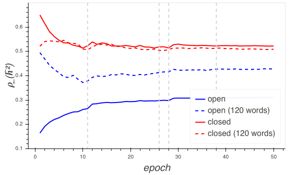
Figure 4: $\rho_{\leftarrow}(\bar{h}^{2})$, evaluated over vocabulary from open and closed classes of POS.

The Role of Part of Speech.

Figure 4 shows that $\rho_{\leftarrow}(\bar{h}^{2})$ follows distinctly different trends for open POS classes and closed classes. To associate words to POS, we tagged our training corpus with spacy; we associate a word to a POS only if the majority (at least 100) of its occurrences are tagged with that POS. We see that initially, frequent words from closed classes are highly concentrated, but soon stabilize, while frequent words from open classes continue to become more concentrated throughout training. Why?

Closed class words clearly signal POS. But open classes contain many ambiguous words, like “report”, which can be a noun or verb. Open classes also contain many more words in general. We posit that early in training, closed classes reliably signal syntactic structure, and are essential for shaping network structure. But open classes are essential for predicting specific words, so their importance in training continues to increase after part of speech tags are effectively learned.

The high sparsity of function word gradient may be surprising when compared with findings that content words have a greater influence on outputs (Kádár et al., 2016). However, those findings were based on the impact on the vector representation of an entire sentence after omitting the word. Khandelwal et al. (2018) found that content words have a longer window during which they are relevant, which may explain the results of Kádár et al. (2016). Neither of these studies controlled for word frequency in their analyses contrasting content and function words, but we believe this oversight is alleviated in our work by measuring correlations rather than raw magnitude. Because $\rho_{\leftarrow}(\bar{h}^{2})$ is higher when evaluated over more frequent words, which also tend to be function words (see Figure 5), we further control for the effect of frequency by including a measurement of trends in a sample of 120 words each from open and closed classes (Figure 4). This sample was selected by sorting all open and closed class words by frequency, then choosing a range of each sorted list with a similar average frequency.

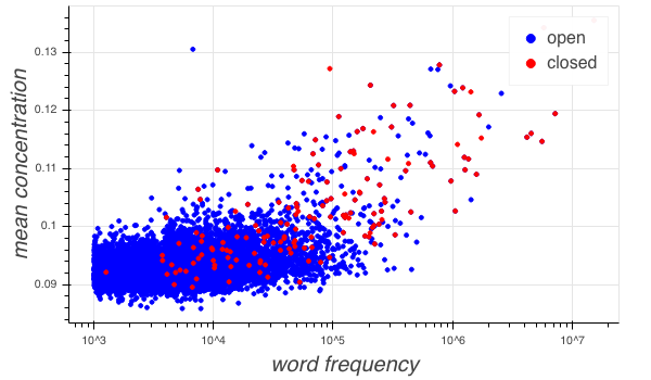
Figure 5: Mean sparsity of $\chi(\bar{h}^{2})$ after 50 epochs, for words occurring more than 1k times in the train set.

Representations of Input Words.

We next looked at the vector representations of each step in the word sequence as a representation of the input word $x_{t-1}$ that produced that step. We measure the correlation with input word frequency:

$$\rho_{\rightarrow}(h)=\textrm{corr}_{w}(\mu_{t:x_{t-1}=w}(\chi(h_{t})),\textrm{freq}(w))$$

Here (Figure 3(b)) we find that the view across training sheds some light on the learning process. While the lower recurrent layer quickly learns sparse representations of common input words, $\rho_{\rightarrow}(h^{1})$ increases more slowly later in training and is eventually surpassed by $\rho_{\rightarrow}(h^{\textrm{e}})$, while gradient sparsity never becomes significantly correlated with word frequency. Li et al. (2016) studied the activations of feedforward networks in terms of the importance of individual units by erasing a particular dimension and measuring the difference in log likelihood of the target class. They found that importance is concentrated into a small number of units at the lowest layers in a neural network, and is more dispersed at higher layers. Our findings suggest that this effect may be a natural result of the sparsity of the activations at lower layers.

We relate the trajectory over training to the Information Bottleneck Hypothesis of Shwartz-Ziv and Tishby (2017). This theory, connected to language model training by Saphra and Lopez (2018), proposes that the earlier stages of training are dedicated to learning to effectively represent inputs, while later in training these representations are compressed and the optimizer removes input information extraneous to the task of predicting outputs. If extraneous information is encoded in specific units, this compression would lead to the observed effect, in which the first time the optimizer rescales the step size, it begins an upward trend in $\rho_{\rightarrow}$ as extraneous units are mitigated.

4 Potential Explanations

Why do common target words have such concentrated gradients with respect to the final LSTM layer? A tempting explanation is that the amount of information we have about common words offers high confidence and stabilizes most of the weights, leading to generally smaller gradients. If this were true, the denominator of sparsity, gradient $\ell_{1}$, should be strongly anti-correlated with word frequency. In fact, it is only ever slightly anti-correlated (correlation $>-.1$). Furthermore, the sparsity of the softmax gradient $\chi(\bar{x})$ does not exhibit the strong correlation seen in $\chi(\bar{h}^{2})$, so sparsity at the LSTM gradient is not a direct effect of sparse logits.

However, the model could still be “high confidence” in terms of how it assigns blame for error during common events, even if it is barely more confident overall in its predictions. According to this hypothesis, a few specialized neurons might be responsible for the handling of such words.

Perhaps common words play a prototyping role that defines clusters of other words, and therefore have a larger impact on these clusters by acting as attractors within the representation space early on. Such a process would be similar to how humans acquire language by learning to use words like ‘dog’ before similar but less prototypical words like ‘canine’ (Rosch, 1999). As a possible mechanism for prototyping with individual units, Dalvi et al. (2019) found that some neurons in a translation system specialized in particular word forms, such as verb inflection or comparative and superlative adjectives. For example, a common comparative adjective like ‘better’ might be used as a reliable signal to shape the handling of comparatives by triggering specialized units, while rarer words have representations that are more distributed according to a small collection of specific contexts.

There may also be some other reason that common words interact more with specific substructures within the network. For example, it could be related to the use of context. Because rare words use more context than common words and content words use more context than function words (Khandelwal et al., 2018), the gradient associated with a common word would be focused on interactions with the most recent words. This would lead common word gradients to be more concentrated.

It is possible that frequent words have sparse activations because frequency is learned as a feature and thus is counted by a few dimensions of proportional magnitude, as posited by Li et al. (2016).

5 Potential Applications

Understanding where natural sparsity emerges in dense networks could be a useful guide in deciding which layers we can apply sparsity constraints to without affecting model performance, for the purpose of interpretability or efficiency. It might also explain why certain techniques are effective: for example, in some applications, summing representations together works quite well Hill et al. (2016). We hypothesize that this occurs when the summed representations are sparse so there is often little overlap. Understanding sparsity could help identify cases where such simple ensembling approaches are likely to be effective.

Future work may develop ways of manipulating the training regime, as in curriculum learning, to accelerate the concentration of common words or incorporating concentration into the training objective as a regularizer. We would also like to see how sparsity emerges in models designed for specific end tasks, and to see whether concentration is a useful measure for the information compression predicted by the Information Bottleneck.

References

- Chen et al. (2016) Yunchuan Chen, Lili Mou, Yan Xu, Ge Li, and Zhi Jin. 2016. Compressing neural language models by sparse word representations. arXiv preprint arXiv:1610.03950.
- Cotterell and Eisner (2018) Ryan Cotterell and Jason Eisner. 2018. A deep generative model of vowel formant typology. arXiv preprint arXiv:1807.02745.
- Dalvi et al. (2019) Fahim Dalvi, Nadir Durrani, Hassan Sajjad, Yonatan Belinkov, Anthony Bau, and James Glass. 2019. What is one grain of sand in the desert? analyzing individual neurons in deep nlp models. In Proceedings of the AAAI Conference on Artificial Intelligence (AAAI).
- Hill et al. (2016) Felix Hill, Kyunghyun Cho, Anna Korhonen, and Yoshua Bengio. 2016. Learning to understand phrases by embedding the dictionary. Transactions of the Association for Computational Linguistics, 4:17–30.
- Hoyer (2004) Patrik O Hoyer. 2004. Non-negative matrix factorization with sparseness constraints. Journal of machine learning research, 5(Nov):1457–1469.
- Karpathy et al. (2015) Andrej Karpathy, Justin Johnson, and Li Fei-Fei. 2015. Visualizing and Understanding Recurrent Networks. arXiv:1506.02078 [cs]. ArXiv: 1506.02078.
- Khandelwal et al. (2018) Urvashi Khandelwal, He He, Peng Qi, and Dan Jurafsky. 2018. Sharp Nearby, Fuzzy Far Away: How Neural Language Models Use Context. arXiv:1805.04623 [cs]. ArXiv: 1805.04623.
- Kádár et al. (2016) Ákos Kádár, Grzegorz Chrupała, and Afra Alishahi. 2016. Representation of linguistic form and function in recurrent neural networks. arXiv:1602.08952 [cs]. ArXiv: 1602.08952.
- Li et al. (2015) Jiwei Li, Xinlei Chen, Eduard Hovy, and Dan Jurafsky. 2015. Visualizing and understanding neural models in NLP. arXiv preprint arXiv:1506.01066.
- Li et al. (2016) Jiwei Li, Will Monroe, and Dan Jurafsky. 2016. Understanding neural networks through representation erasure. arXiv preprint arXiv:1612.08220.
- Murphy et al. (2012) Brian Murphy, Partha Talukdar, and Tom Mitchell. 2012. Learning effective and interpretable semantic models using non-negative sparse embedding. Proceedings of COLING 2012, pages 1933–1950.
- Narang et al. (2017a) Sharan Narang, Gregory Diamos, Shubho Sengupta, and Erich Elsen. 2017a. Exploring Sparsity in Recurrent Neural Networks. arXiv:1704.05119 [cs]. ArXiv: 1704.05119.
- Narang et al. (2017b) Sharan Narang, Erich Elsen, Gregory Diamos, and Shubho Sengupta. 2017b. Exploring sparsity in recurrent neural networks. arXiv preprint arXiv:1704.05119.
- Niculae and Blondel (2017) Vlad Niculae and Mathieu Blondel. 2017. A regularized framework for sparse and structured neural attention. In Advances in Neural Information Processing Systems, pages 3338–3348.
- Padó and Lapata (2007) Sebastian Padó and Mirella Lapata. 2007. Dependency-based construction of semantic space models. Computational Linguistics, 33(2):161–199.
- Pham et al. (2017) Mai Quyen Pham, Benoit Oudompheng, Jérôme I Mars, and Barbara Nicolas. 2017. A noise-robust method with smoothed regularization for sparse moving-source mapping. Signal Processing, 135:96–106.
- Radford et al. (2017) Alec Radford, Rafal Jozefowicz, and Ilya Sutskever. 2017. Learning to Generate Reviews and Discovering Sentiment. arXiv:1704.01444 [cs]. ArXiv: 1704.01444.
- Repetti et al. (2015) Audrey Repetti, Mai Quyen Pham, Laurent Duval, Emilie Chouzenoux, and Jean-Christophe Pesquet. 2015. Euclid in a taxicab: Sparse blind deconvolution with smoothed regularization. IEEE Signal Processing Letters, 22(5):539–543.
- Rosch (1999) Eleanor Rosch. 1999. Principles of categorization. Concepts: core readings, 189.
- Saphra and Lopez (2018) Naomi Saphra and Adam Lopez. 2018. Understanding learning dynamics of language models with svcca. arXiv preprint arXiv:1811.00225.
- Shwartz-Ziv and Tishby (2017) Ravid Shwartz-Ziv and Naftali Tishby. 2017. Opening the Black Box of Deep Neural Networks via Information. arXiv:1703.00810 [cs]. ArXiv: 1703.00810.
- Subramanian et al. (2018) Anant Subramanian, Danish Pruthi, Harsh Jhamtani, Taylor Berg-Kirkpatrick, and Eduard Hovy. 2018. Spine: Sparse interpretable neural embeddings. In Thirty-Second AAAI Conference on Artificial Intelligence.
- Yin et al. (2014) Penghang Yin, Ernie Esser, and Jack Xin. 2014. Ratio and difference of l1 and l2 norms and sparse representation with coherent dictionaries. Commun. Inform. Systems, 14(2):87–109.
- Zibulevsky and Pearlmutter (2001) Michael Zibulevsky and Barak A Pearlmutter. 2001. Blind source separation by sparse decomposition in a signal dictionary. Neural computation, 13(4):863–882.