A Photometric and Spectroscopic Investigation of the DB White Dwarf Population using SDSS and Gaia Data

Abstract

We present a comprehensive analysis of DB white dwarfs drawn from the Sloan Digital Sky Survey, based on model fits to $ugriz$ photometry and medium resolution spectroscopy from the SDSS. We also take advantage of the exquisite trigonometric parallax measurements recently obtained by the Gaia mission. Using the so-called photometric and spectroscopic techniques, we measure the atmospheric and physical parameters of each object in our sample ($T_{\rm eff}$, $\log\textsl{{g}}$, ${\rm H}/{\rm He}$, Ca/He, $R$, $M$), and compare the values obtained from both techniques in order to assess the precision and accuracy of each method. We then explore in great detail the surface gravity, stellar mass, and hydrogen abundance distributions of DB white dwarfs as a function of effective temperature. We present some clear evidence for a large population of unresolved double degenerate binaries composed of DB+DB and even DB+DA white dwarfs. In the light of our results, we finally discuss the spectral evolution of DB white dwarfs, in particular the evolution of the DB-to-DA ratio as a function of $T_{\rm eff}$, and we revisit the question of the origin of hydrogen in DBA white dwarfs.

1 Introduction

The Sloan Digital Sky Survey (SDSS) has dramatically changed our view of white dwarf stars by not only increasing the number of known degenerates by a factor of more than 10, but also by providing a set of homogeneous spectroscopic and photometric observations (Abazajian et al., 2003). More recently, another major milestone has been achieved by the Gaia mission (Gaia Collaboration et al., 2018), which provided accurate trigonometric parallax measurements for 260,000 white dwarfs, and white dwarf candidates (Gentile Fusillo et al., 2019). These accurate distances, coupled with large photometric surveys such as SDSS, Gaia, or Pan-STARRS, open an all new window on the measurement of white dwarf parameters (Gentile Fusillo et al., 2019; Tremblay et al., 2019; Genest-Beaulieu & Bergeron, 2019; Bergeron et al., 2019). In Genest-Beaulieu & Bergeron (2019, hereafter GBB19), we presented a detailed comparison of white dwarf parameters obtained with the so-called spectroscopic and photometric techniques for both DA and DB stars (see also Genest-Beaulieu & Bergeron 2014 and Tremblay et al. 2019). In this paper, we want to focus more specifically on the origin and formation of DB white dwarfs.

While a countless number of spectroscopic analyses of DA white dwarfs has been published in the literature (Bergeron et al. 1992, Liebert et al. 2005, Koester et al. 2009, and Gianninas et al. 2011, just to name a few), only a few are available for DB stars (Eisenstein et al., 2006a; Voss et al., 2007; Bergeron et al., 2011; Koester & Kepler, 2015; Rolland et al., 2018). More importantly, while the atmospheric parameters for DA white dwarfs agree generally well between these various analyses, those of DB stars show larger discrepancies, which can probably be traced back to differences in model atmospheres and fitting techniques. For instance, the treatment of van der Waals broadening remains one of the largest source of uncertainty at low effective temperatures ($T_{\rm eff}\lesssim 16,000$ K; GBB19 and references therein). Also of importance is the assumed convective efficiency at high temperatures ($T_{\rm eff}\sim 25,000$ K), or even the validity of the mixing-length theory used so far in all model atmosphere calculations for DB stars. Cukanovaite et al. (2018) indeed showed that 3D hydrodynamical effects, similar to those found in the context of DA stars (Tremblay et al., 2013a, b), should be equally important for DB white dwarfs. Hence, despite all these efforts, our understanding of the effective temperature, stellar mass, and hydrogen abundance distributions of DB white dwarfs remains sketchy at best. For instance, there are still unanswered questions regarding the mass distribution of DB versus DBA white dwarfs, or the reality of low- and high-mass DB white dwarfs, or even the existence of unresolved double degenerate binaries among the DB population.

Many open questions also remain concerning the origin of DB white dwarfs. There is now little doubt that most DB white dwarfs have evolved from the transformation of DA stars through a process referred to as convective dilution, where the thin hydrogen surface layer ($M_{\rm H}\sim 10^{-16}-10^{-14}M_{\odot}$) of the DA progenitor is gradually eroded and thoroughly mixed with the underlying helium convection zone. However, the details of this mixing process, and in particular the temperature at which it takes place, remain poorly understood (MacDonald & Vennes, 1991; Rolland et al., 2018). There is also the question of the existence of the DB-gap, a region between $T_{\rm eff}\sim 45,000$ K and 30,000 K originally believed to be devoid of helium-atmosphere white dwarfs (Liebert et al., 1986; Fontaine & Wesemael, 1987). It is this particular feature that actually led to the interpretation of the DA-to-DB transition at the red edge of the gap. Now thanks to the SDSS, this gap has been partially filled by hot DB stars (Eisenstein et al., 2006a; Koester & Kepler, 2015), but a strong deficiency of helium-atmosphere white dwarfs still remains in this temperature range, and the exact fraction is uncertain due, once again, to inaccuracies in the temperature scale of hot DB stars.

Important insight can also be gained from a careful determination of the ratio of DB to DA stars as a function of effective temperature, ideally in a volume-limited sample to avoid all possible selection biases. Since the convective dilution process is a strongly-dependent function of the thickness of the hydrogen layer, one could in principle map the hydrogen layer mass ($M_{\rm H}$) in DA stars that turned into DB white dwarfs, by carefully comparing their respective luminosity functions. For instance, Bergeron et al. (2011, see their Figure 24) used the DA and DB white dwarfs identified in the Palomar-Green (PG) survey to show that the DA-to-DB transition occurred for most objects around $T_{\rm eff}\sim 20,000$ K, instead of the canonical value of 30,000 K, an estimate originally based of the location of the red edge of the DB gap. This result led the authors to suggest that a fraction of DB stars may have preserved a helium-rich atmosphere throughout their lifetime, an interpretation certainly supported by the existence of hot, helium-atmosphere white dwarfs in the DB gap.

Another topic of importance is related to the presence of hydrogen in DB white dwarfs — the DBA stars. Hydrogen is detected at the photosphere of a significant fraction of DB stars — mostly through spectroscopic observations at H$\alpha$ —, although the exact fraction varies from study to study depending on the quality of the observations, and most importantly the signal-to-noise ratio (S/N). For instance, Bergeron et al. (2011) found that 44% of their sample of 108 objects showed hydrogen, but further spectroscopic observations at H$\alpha$ of the same sample by Rolland et al. (2018) increased this ratio to 63%. On the other hand, Koester & Kepler (2015) estimated that this fraction could be as high as 75% based on the best spectroscopic data in the SDSS.

An important controversy in the literature also has to do with the origin of hydrogen in these DBA white dwarfs. One possible explanation is that hydrogen has a residual origin, resulting from the convective dilution of the thin hydrogen layer with the more massive helium convection zone. However, the total mass of hydrogen within the mixed H/He convection zone, inferred from the observed hydrogen abundance at the photosphere, is so large — of the order of $M_{\rm H}=10^{-12}~{}M_{\odot}$ — that a DA progenitor with such a massive hydrogen layer would have never mixed in the first place. Or put differently, the thickness of the hydrogen layer required for the convective dilution process to occur would yield photospheric hydrogen abundances that are orders of magnitudes smaller than those observed in DBA white dwarfs.

One possible solution to this problem is to have an external source of hydrogen that would increase its photospheric abundance significantly, assuming mixing has already occurred. Many external sources have been proposed in the literature, including accretion from the interstellar medium (MacDonald & Vennes, 1991), from comets (Veras et al., 2014), or even from disrupted planets (Raddi et al., 2015; Gentile Fusillo et al., 2017). One problem with this interpretation, however, is that the average hydrogen accretion rate required to account for the observed abundances in DBA white dwarfs, would build over time a hydrogen layer at the surface of the DA progenitor thick enough, that such a DA star would never undergo the DA-to-DB transition (Rolland et al., 2018). Also, one would have to explain the existence of DB stars with no detectable traces of hydrogen, in particular at low temperatures where small traces of hydrogen ($\log{\rm H}/{\rm He}\sim-6$) can be easily detected. Nevertheless, there are obvious cases of DBA stars with extremely large abundances of hydrogen and metals (SDSS J124231.07+522626.6, GD 16, GD 17, GD 61, and GD 362; see Gentile Fusillo et al. 2017 and references therein), for which the interpretation in terms of accretion of water-rich asteroid debris cannot be questioned. Gentile Fusillo et al. (2017) even discuss a possible correlation between the presence of hydrogen and metals in DBA white dwarfs, suggesting that some fraction of the hydrogen detected in many, perhaps most, helium-atmosphere white dwarfs is accreted alongside metal pollutants.

In order to shed some light on several of the issues discussed above, we present in this paper a thorough photometric and spectroscopic analysis of the DB white dwarfs identified in the SDSS. We first describe in Section 2 the DB white dwarf sample drawn from the SDSS database, including the spectroscopic, photometric, and astrometric observations, which will be analyzed using the theoretical framework outlined in Section 3. We also explore at length in Section 4 the error budget of our analysis. We then present in Section 5 the results of the atmospheric and physical parameters of all DB white dwarfs in our sample, while objects of particular astrophysical interest are discussed in Section 6. Finally, in the light of our results, we discuss in detail the spectral evolution of DB white dwarfs in Section 7. Some concluding remarks follow in Section 8.

2 DB White Dwarf Sample

The first step of our investigation is to perform a full model atmosphere analysis of DB white dwarfs using the photometric and spectroscopic data from the SDSS database, as well as the trigonometric parallaxes from the Gaia survey. We describe these spectroscopic, photometric, and astrometric samples in turn.

2.1 Spectroscopic Sample

We retrieved the observed spectra of all the spectroscopically identified DB white dwarfs in the SDSS, up to the DR12 (Kleinman et al., 2013; Kepler et al., 2015, 2016). Since we want to characterize the entire population of DB white dwarfs, we kept every subtype in our sample and did not apply any criterion on the S/N value, but a visual inspection of the spectroscopic fits allowed us to removed any problematic data. We did however remove all objects with a spectral type indicating a companion (M or +). Our final spectroscopic sample is composed of 2058 spectra, representing 1915 individual white dwarfs, since 128 of these have multiple spectroscopic observations. Except in Section 4.2, where each spectrum will be treated as an independent object, we will retain only the best ${\rm S/N}$ spectrum of each object for our model atmosphere analysis.

Of the 1915 individual white dwarfs, 1522 (or 79.4%) are classified as DB, including the DB stars showing traces of hydrogen (DBA) and/or metals (DBZ), while the other 20.6% (394 objects) is composed of all other subtypes, including magnetic objects (H), spectra with carbon features (Q), and uncertain spectral types (:). Even though our spectroscopic solution for these other subtypes might be uncertain, it should not impact our conclusion significantly since they represent only a small fraction of the entire sample. The S/N distribution of our spectroscopic sample is presented in Figure 1.

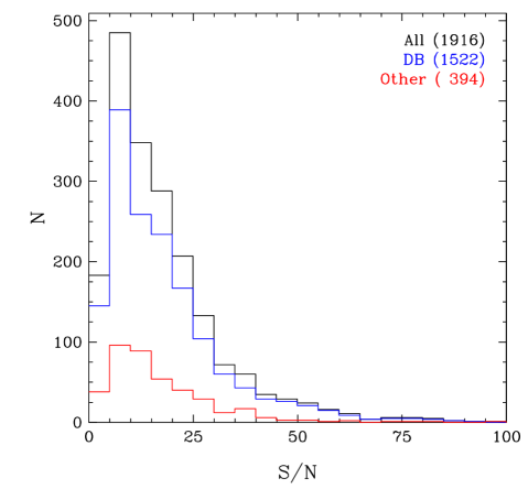
Figure 1: Distribution of S/N of the complete spectroscopic sample (black), the DB subsample (blue), including the DB white dwarfs showing traces of hydrogen (DBA) and/or metals (DBZ), and other subtypes (red).

2.2 Photometric and Astrometric Sample

Since an independent determination of the physical parameters can be obtained from photometry, we also retrieved the $ugriz$ magnitudes for all objects in our spectroscopic sample. We rely on the $ugriz$ photometric data from the SDSS 14^th data release (DR14), since the calibration algorithm has been improved between DR7 and DR8, and the $ugriz$ zero-points have been recalibrated in DR13 as well. We also want to take advantage of the Gaia  DR2 catalog (Gaia Collaboration et al., 2018), which provides precise trigonometric parallax measurements for around 260,000 high confidence white dwarf candidates (Gentile Fusillo et al., 2019), and we thus retrieved the parallaxes for all DB stars in our SDSS sample, if available (about 90% of the objects in our spectroscopic sample). Again here, we applied no specific selection criteria on the quality of the $ugriz$ photometry or on the trigonometric parallaxes, but we visually inspected all photometric fits, and removed any obvious bad photometric or parallax data. As before, we also removed all spectral types containing an M or a +. Our final photometric sample is composed of 1669 photometric data sets, of which 1350 (or $80.9\%$) are DB stars, including spectral types indicating the presence of hydrogen (DBA) and/or metals (DBZ); the other 19.1% (319 photometric sets) is composed of all other subtypes already mentioned above.

The distribution of white dwarfs in our sample as a function of distance and spectral type is presented in Figure 2. As can be seen, most objects are located at very large distances ($D>100$ pc), which implies that their observed $ugriz$ magnitudes will be significantly affected by interstellar reddening. Interstellar extinction will be treated here (see also GBB19 and Bergeron et al. 2019) following the procedure outlined in Harris et al. (2006), where the extinction is considered negligible if $D\leq 100$ pc, to be maximum for the objects located at $|z|>250$ pc from the galactic plane, and to vary linearly between these two regimes.

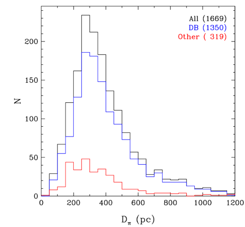
Figure 2: Distribution of parallactic distances for the complete photometric sample (black), the DB and DBA subsample (blue), and the other subtypes (red).

3 Theoretical Framework

The grid of model atmospheres used in the following photometric and spectroscopic analyses is similar to that described in Bergeron et al. (2011), except for the treatment of van der Waals broadening. We use here a treatment based on Deridder & van Rensbergen (1976) instead of Unsold (1955); see Sections 3.2 and 5.2 of GBB19 for details. These models are in LTE and convection is treated with the ML2/$\alpha$=1.25 version of the mixing-length theory (MLT). Our grid covers a range of effective temperatures from 11,000 K to 50,000 K, surface gravities from $\log\textsl{{g}}=7.0$ to $9.0$, and hydrogen abundances (in number) from $\log{\rm H}/{\rm He}=-6.5$ to $-2.0$, as well as a pure helium grid. Additional models have also been calculated that include the Ca ii H and K doublet, in order to properly fit the white dwarfs in our sample showing strong calcium lines. This smaller grid is similar to that described in Bergeron et al. (2011) — except again for the treatment of van der Waals broadening — and covers a range of $T_{\rm eff}=12,000~{}{\rm K}$ to 19,000 K, calcium abundances of $\log{\rm Ca}/{\rm He}=-7.5$, $-7.0$, $-6.5$, and $-6.0$, and the same range of $\log\textsl{{g}}$ and ${\rm H}/{\rm He}$ values as before.

To determine the atmospheric and physical parameters of the DB white dwarfs in our sample, we rely on the photometric and spectroscopic techniques described at length in GBB19 and references therein. Briefly, with the photometric approach, the effective temperature $T_{\rm eff}$ and solid angle $\pi(R/D)^{2}$ are obtained by comparing the observed energy distribution — built from the $ugriz$ photometry — with the predictions of model atmospheres, while with the spectroscopic method, $T_{\rm eff}$, the surface gravity $\log\textsl{{g}}$, and the hydrogen abundance ${\rm H}/{\rm He}$ are obtained by comparing the observed and synthetic spectra, both normalized to a continuum set to unity. Stellar masses can then be derived from evolutionary models. We rely here on C/O-core envelope models similar to those described in Fontaine et al. (2001) with thin hydrogen layers of $q({\rm H})\equiv M_{\rm H}/M_{\star}=10^{-10}$, which are representative of helium-atmosphere white dwarfs. For the DB stars in our sample showing calcium lines, we explore the spectroscopic fits obtained for each calcium abundance in our grid, and adopt the solution with the lowest $\chi^{2}$ value.

4 Error Estimation

As discussed in the Introduction, our understanding of the nature and evolution of DB white dwarfs rests heavily on our ability to measure their atmospheric and physical parameters with great accuracy and precision. We thus present in this section a thorough analysis of the photometric and spectroscopic errors associated with the determinations of white dwarf parameters.

4.1 Photometric Errors

The errors associated with our photometric solutions can be obtained directly from the covariance matrix of the Levenberg-Marquadt minimization procedure used in the photometric technique. These depend mostly on the uncertainty associated with the observed magnitudes and the sensitivity of the $ugriz$ photometry to the atmospheric parameters. We apply here a lower limit of 0.03 mag on each bandpass so that the photometric solution is not driven by a single magnitude with an extremely small uncertainty (see also Bergeron et al. 2019). As also discussed in Bergeron et al. (2019), the SDSS magnitude system is not exactly on the AB magnitude system, and corrections of the order of 0.03 mag must be added to some bandpasses, all of which remain uncertain. Since we use the trigonometric parallax in the fitting procedure, the errors on the atmospheric parameters will depend on $\sigma_{\pi}$ as well. Note that all values reported in this section are for the DB stars only, and we expect our errors for other subtypes (e.g. magnetic DB stars or uncertain spectral types) to be even larger.

The errors associated with our photometric effective temperatures are presented in the top panel of Figure 3. The mean error for the overall sample is $\sim$10% in $T_{\rm eff}$, but the individual errors vary significantly as a function of temperature since they widely depend on the sensitivity of the $ugriz$ photometry to variations in $T_{\rm eff}$ (see Figure 4 of GBB19). For instance, the errors drop significantly below $\sim$16,000 K, where the $ugriz$ photometry is very sensitive to $T_{\rm eff}$, reaching values as small as 2% near 10,000 K. More puzzling is the significant increase in $\sigma_{T_{\rm eff}}$ in the range $26,000~{}{\rm K}>T_{\rm eff}>22,000~{}{\rm K}$. We traced back this feature — never discussed in the literature, to our knowledge — to the particular behavior of the Eddington fluxes in the optical regions, which increase very slowly in this temperature range, when the main opacity source switches from the He i bound-free opacity to the He ii free-free opacity, as illustrated in Figure 4. Finally, $\sigma_{T_{\rm eff}}$ does not appear to be significantly affected by the parallax uncertainties $\sigma_{\pi}$. If we restrict our sample to the objects for which $\sigma_{\pi}/\pi<0.25$, we obtain $\langle\sigma_{T_{\rm eff}}\rangle=8.7\%$, a value only slightly lower than that obtained above. This is an expected result since $T_{\rm eff}$ is determined mainly from the shape of the energy distribution, which does not depend on the parallactic distance (after dereddening).

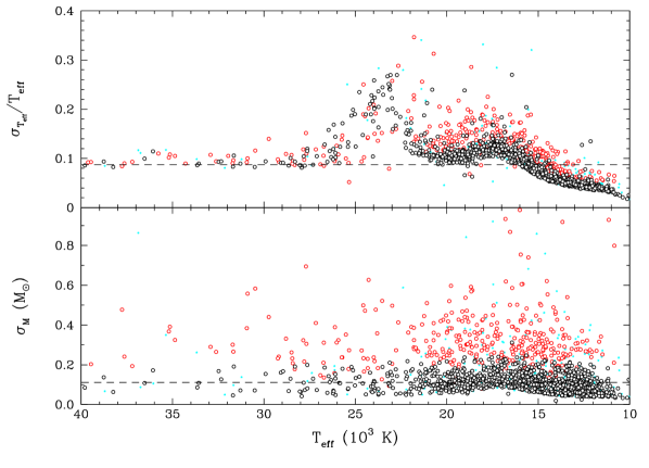
Figure 3: Distribution of errors on $T_{\rm eff}$ (top panel) and stellar mass (bottom panel) obtained from the photometric technique, as a function of effective temperature. The open circles represent the DB and DBA stars in our sample with $\sigma_{\pi}/\pi<0.25$ (black) and $\sigma_{\pi}/\pi>0.25$ (red). The dashed lines indicate the mean errors of the DB/DBA photometric subsample with $\sigma_{\pi}/\pi<0.25$. All other spectral types are represented by cyan dots.

Figure 4: Eddington fluxes (in units of ergs cm^-2 s^-1 Hz^-1) as a function of wavelength for pure helium DB models at $\log\textsl{{g}}=8$, and for various effective temperatures (in units of $10^{3}$ K) indicated in the figure.

The errors associated with photometric masses are presented in the bottom panel of Figure 3. The mean error for the overall sample is somewhat high, $\langle\sigma_{M}\rangle=0.341$ $M_{\odot}$, but this is mostly caused by the objects in our sample with very large parallax uncertainties. Unlike for the effective temperature, the precision on the mass relies heavily on $\sigma_{\pi}$ since the parallactic distance is used to obtain the radius from the solid angle, which is then converted into mass using the mass-radius relation (see section 4.1 of GBB19). If we restrict our sample to objects with $\sigma_{\pi}/\pi<0.25$, we obtain a much lower mean value for the error of $\langle\sigma_{M}\rangle=0.112~{}M_{\odot}$. We also note that the $\sigma_{M}$ distribution in Figure 3 is fairly constant with effective temperature, unlike what is observed for $\sigma_{T_{\rm eff}}$.

Finally, if we do not apply the 0.03 mag lower limit uncertainty on the $ugriz$ magnitudes, the mean uncertainties are only slightly lower: $\langle\sigma_{T_{\rm eff}}\rangle=6.85\%$ and $\langle\sigma_{M}\rangle=0.102~{}M_{\odot}$ (for $\sigma_{\pi}/\pi<0.25$).

4.2 Spectroscopic Errors

The spectroscopic errors associated with the atmospheric parameters — $T_{\rm eff}$, $\log\textsl{{g}}$, and ${\rm H}/{\rm He}$ — can be estimated from the covariance matrix of the Levenberg-Marquadt procedure used in our fitting technique. These so-called internal errors represent the ability of our models to reproduce the data, and can be made arbitrarily small if the ${\rm S/N}$ of the spectra is high enough (see Liebert et al. 2005 for a full discussion). The internal errors on $T_{\rm eff}$, $\log\textsl{{g}}$, and ${\rm H}/{\rm He}$ are displayed in Figure 5 as a function of effective temperature, together with the errors on the spectroscopic mass, obtained by combining the effects of $\sigma_{T_{\rm eff}}$ and $\sigma_{\log\textsl{{g}}}$ on the mass determination (note that $\sigma_{M}$ is completely dominated by the contribution of $\sigma_{\log\textsl{{g}}}$, however).

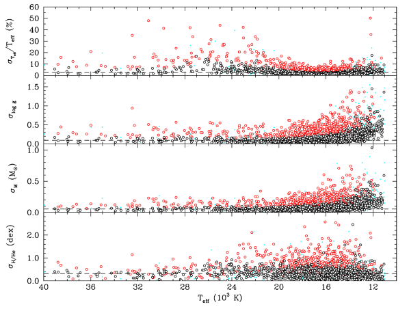
Figure 5: Internal errors on $T_{\rm eff}$, $\log\textsl{{g}}$, $M$, and ${\rm H}/{\rm He}$ obtained from the spectroscopic technique, as a function of effective temperature. The open circles represent the DB(Z) and DBA(Z) white dwarfs with ${\rm S/N}>10$ (black) and ${\rm S/N}<10$ (red); all other subtypes are represented by cyan dots. The dashed lines indicate the corresponding mean errors for the objects with ${\rm S/N}>10$, and $T_{\rm eff}>16,000$ K for $\sigma_{\log\textsl{{g}}}$ and $\sigma_{M}$.

The mean error on $T_{\rm eff}$ for the overall sample is $\langle\sigma_{T_{\rm eff}}\rangle=4.43\%$, or 2.59% if we restrict our sample to ${\rm S/N}>10$. The individual errors $\sigma_{T_{\rm eff}}$ (in percentage) are fairly constant with effective temperature, except between $\sim$20,000 K and 30,000 K where the helium lines become less sensitive to $T_{\rm eff}$ (see Figure 1 of Bergeron et al. 2011). The mean error on $\log g$ is $\langle\sigma_{\log\textsl{{g}}}\rangle=0.263$, and on the mass $\langle\sigma_{M}\rangle=0.156~{}M_{\odot}$; these values drop to 0.163 and $0.088~{}M_{\odot}$, respectively, if we restrict our sample to ${\rm S/N}>10$. Unlike for $\sigma_{T_{\rm eff}}$, there is no increased scatter in the distributions between 20,000 K and 30,000 K, indicating that the helium lines remain sensitive to $\log g$ and mass in this temperature range. However, we can see that the individual errors become more important below $T_{\rm eff}\sim 16,000~{}{\rm K}$, where neutral broadening remains a large source of uncertainty in our models (see GBB19 and references therein). If we exclude the objects below $16,000~{}{\rm K}$, the mean errors drop even further to $\langle\sigma_{\log\textsl{{g}}}\rangle=0.094$ and $\langle\sigma_{M}\rangle=0.053~{}M_{\odot}$ (for ${\rm S/N}>10$). Finally, the mean error on the hydrogen abundance is $\langle\sigma_{\rm H/He}\rangle=0.486$ dex (or 0.314 dex for the sample with ${\rm S/N}>10$), but this somewhat large mean value is dominated by the objects for which we could only determine an upper limit on the hydrogen abundance. If we restrict our estimation to the DBA stars in our sample, the mean error drop to 0.298 dex (or 0.213 dex for the sample with ${\rm S/N}>10$).

Another way to estimate the errors using the spectroscopic technique is from multiple observations of the same star, as described for instance in Liebert et al. (2005) and Bergeron et al. (2011). To get a good estimate of the external errors, we excluded all spectra with ${\rm S/N}<10$ as well as uncertain spectral types, which left us with 49 objects with multiple spectra. For those with more than two observations, we kept only the two highest ${\rm S/N}$ spectra. These so-called external errors are displayed in Figure 6. The mean external errors are $\langle\Delta T_{\rm eff}/T_{\rm eff}\rangle=2.40\%$, $\langle\Delta\log\textsl{{g}}\rangle=0.152$, $\langle\Delta M\rangle=0.086$ $M_{\odot}$, and $\langle\Delta{\rm H/He}\rangle=0.199$ dex. These values compare favorably well with the internal errors discussed above. Bergeron et al. (2011) obtained smaller values of $\langle\Delta T_{\rm eff}/T_{\rm eff}\rangle=2.3\%$ and $\langle\log\textsl{{g}}\rangle=0.052$, which can be explained by the fact that the spectra used in their analysis had ${\rm S/N}>50$, while in our restricted sample $\langle{\rm S/N}\rangle\sim 25$ (see Figure 1). Perhaps a more useful comparison is with the values obtained by Koester & Kepler (2015) based on multiple spectra from the SDSS. They obtained similar mean errors of 3.1% in $T_{\rm eff}$, 0.12 in $\log\textsl{{g}}$, and 0.18 dex in ${\rm H}/{\rm He}$.

We reevaluate again in Section 5.5 the precision and accuracy of the photometric and spectroscopic techniques, but only after we compare the atmospheric and physical parameters determined using both fitting methods.

Figure 6: Comparison of $T_{\rm eff}$, $\log\textsl{{g}}$, $M$, and $\log{\rm H}/{\rm He}$ for the 49 objects in our sample with multiple spectroscopic observations and with ${\rm S/N}>10$.

5 Atmospheric and Physical Parameters of DB White Dwarfs

Our main goal is to characterize the entire DB white dwarf population in the SDSS. To do so, we take advantage of the photometric and spectroscopic techniques to obtain independent determinations of the atmospheric and physical parameters of each star, such as the effective temperature $T_{\rm eff}$, the surface gravity $\log\textsl{{g}}$, the stellar mass $M$, and the hydrogen abundance ratio ${\rm H}/{\rm He}$. Note that the latter can only be determined spectroscopically. The derived parameters are provided in Table 1. Even though our sample contains several subtypes, particular attention will be given to the DB and DBA white dwarfs (with or without metals) as these represent about 80% of our sample (see Section 2). In this section, we discuss in turn the surface gravity, stellar mass, and photospheric hydrogen abundance distributions.

Table 1: List of photometric/spectroscopic atmospheric/physical parameters

	Photometry				Spectroscopy
SDSS name	$T_{\rm eff}$	$\log\textsl{{g}}$	$M$	$\sigma_{\pi}/\pi$	$T_{\rm eff}$	$\log\textsl{{g}}$	$M$	$\log{\rm H}/{\rm He}$	$\log{\rm Ca}/{\rm He}$	${\rm S/N}$	Notes
	(K)		($M_{\odot}$)		(K)		($M_{\odot}$)
$000055.12-042449.00$	14,675	7.80	0.483	0.694	13,649	7.88	0.517	$-5.111$	$\cdots$	10.16
$000106.22+250330.00$	15,753	7.03	0.237	0.527	14,836	7.88	0.520	$-4.748$	-7.50	18.68
$000111.66+000342.55$	$\cdots$	$\cdots$	$\cdots$	$\cdots$	11,205	6.32	0.022	$-5.327$	$\cdots$	18.84	1
$000116.49+000204.45$	11,238	7.87	0.510	0.093	11,304	7.73	0.440	$-5.965$	$\cdots$	31.52	1
$000122.51+235934.20$	$\cdots$	$\cdots$	$\cdots$	$\cdots$	12,339	6.88	0.194	$<-5.672$	$\cdots$	7.63	1
$000205.57+002041.80$	19,926	7.11	0.266	1.388	18,108	8.16	0.693	$-5.025$	$\cdots$	6.47
$000223.06+272358.50$	16,437	8.08	0.637	0.033	16,830	8.00	0.594	$<-6.133$	$\cdots$	49.67
$000407.15+264939.70$	12,800	7.96	0.565	0.222	14,050	9.28	1.288	$-5.263$	$\cdots$	9.47
$000426.95+243258.90$	10,564	8.25	0.738	0.173	16,206	9.16	1.253	$-5.090$	-6.00	10.46
$000447.06+240703.60$	$\cdots$	$\cdots$	$\cdots$	$\cdots$	15,328	7.75	0.457	$-5.434$	$\cdots$	9.47
$000509.94+003809.60$	47,176	7.68	0.503	0.278	50,033	7.68	0.509	$<-3.280$	$\cdots$	16.24
$000515.58+071313.71$	17,994	7.90	0.538	0.057	19,000	8.15	0.686	$<-5.600$	$\cdots$	40.62
$000720.22-002325.40$	19,434	8.10	0.658	0.096	19,099	7.90	0.540	$<-5.383$	$\cdots$	18.67
$000730.75+275111.90$	13,932	7.64	0.405	0.250	16,305	8.06	0.629	$-5.880$	$\cdots$	11.92	2
$000731.17-095849.10$	18,651	7.90	0.541	0.326	20,170	8.05	0.625	$<-4.849$	$\cdots$	6.32
$000742.62+252422.50$	20,913	8.64	0.999	0.368	28,723	7.80	0.511	$<-3.702$	$\cdots$	12.85

Note. — Table 1 is published in its entirety in the machine-readable format. A portion is shown here for guidance regarding its form and content.

5.1 Surface Gravity Distributions

We present in Figure 7 the photometric and spectroscopic surface gravities as a function of effective temperature for all DB white dwarfs in our sample. The photometric $\log\textsl{{g}}$ distribution (upper panel) is well centered on the 0.6 $M_{\odot}$ evolutionary sequence at all temperatures, as expected. Moreover, the dispersion in $\log\textsl{{g}}$ values appears fairly constant with $T_{\rm eff}$, and the distribution in temperature is also uniform, in the sense that there are no regions with an obvious accumulation or depletion of objects. The spectroscopic $\log\textsl{{g}}$ distribution (middle panel) is also uniform in temperature, but contrary to the photometric distribution, it deviates significantly from the 0.6 $M_{\odot}$ sequence in several temperature ranges. First, at the very cool end of the distribution ($T_{\rm eff}\lesssim 13,000$ K), the $\log\textsl{{g}}$ values are much lower than the canonical $\log g=8$ value. This behavior can be partially explained by the weakness of the helium lines in this temperature range (see Figure 3 of Rolland et al. 2018), and the spectroscopic technique has most likely reached its limits below which the atmospheric parameters become unreliable. We estimated this limit at the temperature where the equivalent width of the He i $\lambda 4471$ line becomes smaller than 3 Å (4 Å, 5 Å) for ${\rm S/N}>20$ ($10<{\rm S/N}<20$, ${\rm S/N}<10$). These objects are shown as magenta triangles in Figure 7 and will not be considered any further in our analysis.

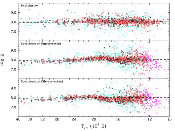
Figure 7: Photometric (upper panel) and spectroscopic (middle panel) $\log\textsl{{g}}$ distributions as a function of $T_{\rm eff}$. The open circles represent the DB (black) and DBA (red), with or without metals, while the black dots correspond to other spectral types with $\sigma_{\pi}/\pi<0.25$ (photometry) or ${\rm S/N}>10$ (spectroscopy). Spectra with marginal helium lines are shown as magenta triangles, and any object with $\sigma_{\pi}/\pi>0.25$ or ${\rm S/N}<10$, regardless of the spectral type, is represented by a cyan dot. Bottom panel: Same as middle panel, but with the 3D hydrodynamical corrections taken into account. In all panels, the dashed line represents a 0.6 $M_{\odot}$ evolutionary sequence.

However, even by removing from the sample these spectra with marginally detectable helium lines, we still see a larger scatter around $T_{\rm eff}\sim 13,000-16,000$ K, in contrast to what is observed in photometry. The main line broadening mechanism in this particular temperature range is the broadening by neutral particles, or more specifically van der Waals broadening. As mentioned in several studies, the large scatter at the cool end of the spectroscopic $\log g$ distribution ($T_{\rm eff}<16,000~{}{\rm K}$) is mostly caused by the improper treatment of van der Waals broadening (Beauchamp et al. 1996; Bergeron et al. 2011; Koester & Kepler 2015; GBB19), and the theory currently used in our model atmospheres probably still requires some improvement in order to determine more accurate $\log\textsl{{g}}$ values below $T_{\rm eff}=16,000~{}{\rm K}$. Nevertheless, we do find convincing cases of white dwarfs in this temperature range with a broad range of spectroscopic $\log\textsl{{g}}$ values. This is illustrated in Figure 8, where we show 3 DB(A) white dwarfs with similar spectroscopic temperatures ($T_{\rm eff}\sim 14,700~{}{\rm K}$), but with different surface gravities, ranging from $\log g=7.7$ to 8.3 (see also Figure 7 of Limoges & Bergeron 2010 and the related discussion). For these 3 objects, the shape and strength of the He i $\lambda$3820 and $\lambda$4388 lines, which are particularly $\log\textsl{{g}}$-sensitive in this temperature regime, vary significantly. We would like to stress that this is independent of any theoretical modeling, since it is observed directly in the spectrum. This suggests that, despite the unsatisfactory treatment of van der Waals broadening, at least part of the scatter in $\log\textsl{{g}}$ observed below $T_{\rm eff}=16,000~{}{\rm K}$ might be real after all. This is supported by the fact that the photometric distribution also shows several high-$\log\textsl{{g}}$ objects. We come back to this point further in Section 5.2.

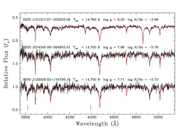
Figure 8: Our best spectroscopic fits to 3 DB(A) white dwarfs near $T_{\rm eff}=14,700~{}{\rm K}$, but with significantly different surface gravities. The spectra have been normalized to a continuum set to unity and the best-fit solutions are shown by the red lines. The atmospheric parameters for each object are indicated as well. The location of He i $\lambda$3820 and $\lambda$4388, which are the most $\log\textsl{{g}}$-sensitive in this temperature regime, is shown by the blue tick marks.

At the hot end ($T_{\rm eff}>27,000~{}{\rm K}$) of the spectroscopic $\log\textsl{{g}}$ distribution in Figure 7, we see also a trend towards lower $\log\textsl{{g}}$ values, with inferred masses below 0.6 $M_{\odot}$, again in sharp contrast with what is observed in photometry. Tremblay et al. (2011) and Genest-Beaulieu & Bergeron (2014) observed a similar phenomenon when analyzing the spectroscopic $\log\textsl{{g}}$ distribution of DA white dwarfs from the SDSS. In this case, a comparison with the DA spectra taken from Gianninas et al. (2011, see for instance Figures 14 and 15 of ), where this effect was not observed, indicated that the apparent decrease in $\log\textsl{{g}}$ when using the SDSS spectra could be attributed to residual flux calibration issues. Since this calibration problem must also affect the spectra of DB white dwarfs, we conclude that the apparent decrease in spectroscopic $\log\textsl{{g}}$ values observed in Figure 7 above $T_{\rm eff}\sim 27,000~{}{\rm K}$ is most likely an artifact caused by calibration issues with the SDSS spectra.

Another possibility, mentioned by Koester & Kepler (2015), is that the cooler white dwarfs might originate from more massive progenitors, since DB stars at $T_{\rm eff}\sim 10,000~{}{\rm K}$ are about $5\times 10^{8}$ years older than those at $T_{\rm eff}\sim 30,000~{}{\rm K}$. They estimated that the hotter stars could be less massive than the cooler ones by about 0.05 $M_{\odot}$, thus explaining the slight decrease in $\log\textsl{{g}}$. However, even though this would be a valid explanation in a stellar cluster where there is a single burst of star formation, it certainly does not apply in the case of field white dwarfs where continuous star formation occurs. And indeed, such an effect in $\log\textsl{{g}}$ (or mass) is not detected in the DA population (see Figure 30 of Gianninas et al. 2011 for instance).

Finally, the spectroscopic $\log\textsl{{g}}$ distribution in Figure 7 also shows a small but significant increase in the range $22,000~{}{\rm K}>T_{\rm eff}>16,000~{}{\rm K}$, also noted by GBB19. In this region, we obtain from spectroscopy $\langle\log\textsl{{g}}\rangle=8.15$ (for ${\rm S/N}>10$), a value slightly larger than that obtained from photometry, $\langle\log\textsl{{g}}\rangle=8.08$ (for $\sigma_{\pi}/\pi<0.25$). This corresponds to the temperature range where the 3D hydrodynamical effects become important according to Cukanovaite et al. (2018), who recently calculated 3D model atmospheres for pure helium-atmosphere white dwarfs. Cukanovaite et al. also published 3D corrections (see their Table 2) to be applied to the 1D spectroscopic solutions (assuming ML2/$\alpha=1.25$), which are reproduced here in Figure 9, for completeness. The largest corrections in $\log\textsl{{g}}$ occur near 17,000 K — which incidentally coincides with the maximum increase in $\log\textsl{{g}}$ observed in the middle panel of Figure 7 —, while the largest corrections in $T_{\rm eff}$ occur at much higher temperatures, near $T_{\rm eff}=25,000~{}{\rm K}$.

The 3D-corrected spectroscopic $\log\textsl{{g}}$ distribution for our sample is displayed in the bottom panel of Figure 7. While the mean $\log\textsl{{g}}$ value between 20,000 K and 22,000 K is now 8.05 — in excellent agreement with the photometric mean — the surface gravities below this temperature range are over-corrected when compared to the photometric results. For instance, between $T_{\rm eff}\sim 15,000~{}{\rm K}$ and 20,000 K, the spectroscopic distribution has a mean value of $\log\textsl{{g}}=7.87$ (for ${\rm S/N}>10$), which is 0.18 dex below the corresponding photometric value, suggesting that the $\log\textsl{{g}}$ corrections in this temperature range are probably overestimated. The 3D corrections in $T_{\rm eff}$ appear problematic as well. Indeed, while the photometric and uncorrected $\log\textsl{{g}}$ distributions are uniform as a function of effective temperature, the corrected spectroscopic distribution now shows an accumulation of objects around 25,000 K, as well as a depletion of objects near 28,000 K.

However, it is important to stress at this point that these 3D corrections are available for pure helium atmospheres only, and it is expected that calculations currently underway, which include the presence of hydrogen, will improve the results. We defer the rest of our discussion of these 3D corrections to the end of the next section.

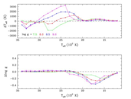
Figure 9: Theoretical 3D hydrodynamical corrections in $T_{\rm eff}$ (top panel) and $\log\textsl{{g}}$ (bottom panel) to be applied to 1D spectroscopic solutions, as a function of effective temperature and for various $\log\textsl{{g}}$ values, as described in Table 2 of Cukanovaite et al. (2018).

5.2 Mass Distributions

The stellar radii and $\log\textsl{{g}}$ values obtained from the photometric and spectroscopic techniques, respectively, can be converted into stellar mass using the evolutionary models described in Section 3. These photometric and spectroscopic masses for all the DB white dwarfs in our sample are displayed in Figure 10 as a function of effective temperature. We focus here on the results from our best data sets, represented by black and red circles for the DB and DBA white dwarfs, respectively. Not unexpectedly, we observe here the same behavior as with the $\log\textsl{{g}}$ distribution. In particular, the photometric mass distribution is well centered at 0.6 $M_{\odot}$, while the spectroscopic distribution exhibits all the pitfalls previously described. Most noteworthy are the spectroscopic masses in the $16,000-22,000$ K temperature range, which are systematically larger than the canonical 0.6 $M_{\odot}$ value, while they appear systematically lower than this value outside this temperature range. As discussed above, these features can be explained as a combination of residual flux calibration problems with the SDSS spectra, 3D hydrodynamical effects, and inadequate van der Waals broadening, which all affect our spectroscopic solutions.

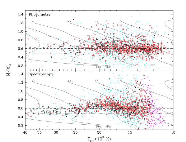
Figure 10: Photometric and spectroscopic masses as a function of effective temperature. The description of symbols is identical to that of Figure 7. Also shown as solid lines are theoretical isochrones obtained from models with C/O cores, $q(\rm{He})=10^{-2}$, and $q(\rm{H})=10^{-10}$, labeled in units of 10⁹ years. The horizontal dotted and dashed lines are located at $M=0.48~{}M_{\odot}$ and $M=0.6~{}M_{\odot}$, respectively (see text).

Another way to investigate the white dwarf masses is to look at the relative mass distributions. To ensure the best possible mass values, we restricted our spectroscopic sample to the objects with ${\rm S/N}>10$, and discarded the spectra showing only marginal helium lines (see Section 5.1). Similarly, for the photometric mass distribution, we restricted our sample to $\sigma_{\pi}/\pi<0.25$. The resulting mass distributions, both photometric and spectroscopic, are displayed in Figure 11. Despite the problems mentioned in the previous paragraph, the relative mass distributions obtained from photometry and spectroscopy are remarkably similar. They both have a mean mass of $\sim$$0.63~{}M_{\odot}$, and very similar dispersions ($\sigma_{M,{\rm phot}}=0.135~{}M_{\odot}$ and $\sigma_{M,{\rm spec}}=0.138~{}M_{\odot}$). These mean masses are much lower than the value of $0.706~{}M_{\odot}$ reported by Koester & Kepler (2015) for their complete sample, which can probably be attributed to differences in model atmospheres and fitting techniques (see Section 5.4). Note, however, that their favored mean mass for DB white dwarfs is $0.606~{}M_{\odot}$, based exclusively on the objects between $T_{\rm eff}=16,000$ K and 22,000 K.

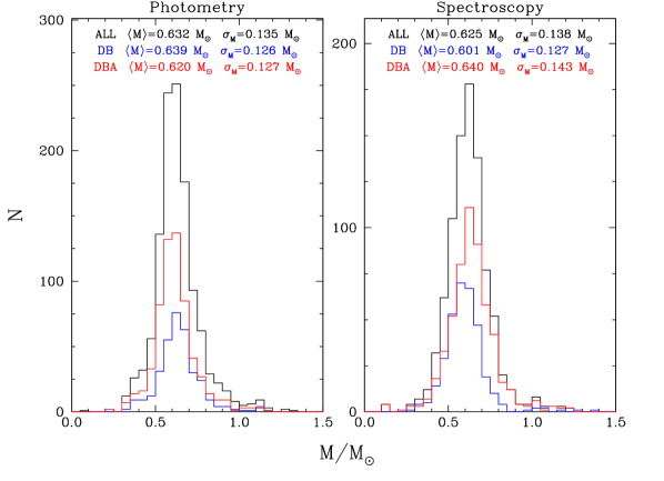
Figure 11: Left: Photometric mass distribution for the objects with $\sigma_{\pi}/\pi<0.25$. Right: Spectroscopic mass distribution for the DB spectra with ${\rm S/N}>10$. The objects with very marginal helium lines have been excluded. Also shown are the corresponding mass distributions for the DB (blue) and DBA (red) subsamples. The mean masses and standard deviations are also given in each panel.

One particular feature often reported regarding the mass distribution of DB white dwarfs is the complete absence of a low-mass tail (Beauchamp et al. 1996; Bergeron et al. 2011; GBB19), suggesting that common envelope evolution scenarios, which are often invoked to explain low-mass ($\lesssim 0.48~{}M_{\odot}$) DA stars (Bergeron et al., 1992), do not produce DB white dwarfs. Our spectroscopic mass distribution displayed in Figure 11 shows a few DB white dwarfs with such low masses, but an examination of Figure 10 (where this low-mass limit is indicated by the dotted line) reveals that these objects are located either below $T_{\rm eff}=16,000~{}{\rm K}$, where our solutions are more uncertain due to the improper treatment of van der Waals broadening, or above $T_{\rm eff}\sim 25,000~{}{\rm K}$, where the calibration issues with the SDSS spectra affect the spectroscopic solutions. The photometric mass distributions in both Figures 10 and 11, which are not affected by these problems, also show several low-mass objects, but these are most likely unresolved double degenerates, as discussed in Section 6.1. Therefore, we find no compelling evidence in our analysis for the existence of low-mass DB white dwarfs, a conclusion also reached by Beauchamp et al. (1996), Bergeron et al. (2011), and GBB19.

The high-mass tail of the spectroscopic mass distribution observed in Figure 11 is often attributed to the improper treatment of van der Waals broadening in model atmospheres (Bergeron et al. 2011; Koester & Kepler 2015; GBB19). This is supported by the fact that most objects with large spectroscopic masses are located below 16,000 K where this type of line broadening dominates (see Figure 10). This might not be the whole story, however, since the photometric mass distribution also shows a similar high-mass tail (see also Figure 10). We present in Figure 12 our best photometric and spectroscopic fits for four massive DB white dwarfs in our sample. In all cases, the photometric and spectroscopic solutions are in good agreement, within the uncertainties. Note also that they are not in the temperature regime where van der Waals broadening dominates. Consequently, their large inferred masses appear real. The existence of massive DA white dwarfs is usually explained by stellar mergers (Iben, 1990; Kilic et al., 2018), or as a result of the initial-to-final mass relation (El-Badry et al., 2018). The same mechanisms can possibly be invoked as well to explain the presence of such massive DB white dwarfs in our sample.

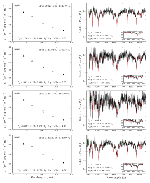
Figure 12: Left: Best photometric fits to four massive DB white dwarfs. The error bars represent the observed $ugriz$ magnitudes and associated uncertainties, while the filled circles represent the best-fit model. Right: Corresponding best spectroscopic fits. The best-fit model (red) is plotted over the normalized observed spectrum (black). The inset shows the region near H$\alpha$ used to determine the hydrogen abundance, or upper limits. The derived atmospheric and physical parameters are also given.

Another possible explanation for the origin of massive DB white dwarfs involves the so-called Hot DQ stars, whose atmospheres are dominated by carbon (Dufour et al., 2007, 2008). Since Hot DQ white dwarfs are only found above $T_{\rm eff}\sim 18,000~{}{\rm K}$, Bergeron et al. (2011) proposed that they somehow transform into DB stars around that temperature, through a currently unknown physical mechanism. An examination of the upper panel of Figure 10 actually reveals that massive DB white dwarfs start to appear below $T_{\rm eff}\sim 22,000~{}{\rm K}$, coinciding with the coolest Hot DQ stars known today. The hot DQs also tend to be massive, since they are most likely the end result of white dwarf mergers (Dunlap & Clemens, 2015). Therefore, we suggest that some of the massive DB white dwarfs observed in our sample could be former Hot DQ stars.

Another particularly important issue is whether the mass distributions of DB and DBA white dwarfs differ or not. In our analysis, we considered an object to be a DB star if the spectroscopic technique could only determine an upper limit on the hydrogen abundance. The relative photometric mass distributions for DB and DBA white dwarfs are presented in the left panel of Figure 11. The comparison indicates that the average masses differ by less than 0.02 $M_{\odot}$, and that their dispersions are identical, a result that is readily apparent when looking at the upper panel of Figure 10. A similar comparison with the spectroscopic mass distributions displayed in the right panel of Figure 11 suggest that DB white dwarfs are slightly less massive than DBA stars, by about 0.04 $M_{\odot}$. However, it is also obvious from the results shown in the lower panel of Figure 10 that these mass differences stem from all the problems related with the spectroscopic technique across the entire temperature range, both observational and theoretical, as already discussed extensively above. We thus conclude that there is no significant mass difference between the DB and DBA white dwarfs, and that the explanation for the origin of hydrogen in DBA stars is not mass related.

Finally, we go back to our discussion of the 3D hydrodynamical corrections by looking at the relative mass distributions. In Figure 13, we compare the photometric masses — which are unaffected by 3D effects — with those obtained spectroscopically, both uncorrected and 3D-corrected. Note that the mass distributions displayed here include only the DB white dwarfs in common with both the photometric and spectroscopic samples. Although the photometric and uncorrected spectroscopic mass distributions overlap almost perfectly, the 3D-corrected distribution is significantly shifted towards lower masses. Its mean mass is $\langle M\rangle=0.55~{}M_{\odot}$, which is $0.06~{}M_{\odot}$ lower than the value inferred from photometry, $\langle M\rangle=0.61~{}M_{\odot}$. This again suggests that the proposed 3D corrections in $\log\textsl{{g}}$ are too strong. As previously mentioned, however, the corrections applied here are appropriate for pure helium models only, and it is possible that 3D hydrodynamical models including traces of hydrogen will yield a more satisfactory agreement. For the time being, since most objects in our sample show traces of hydrogen, we will refrain from applying the 3D corrections to our spectroscopic parameters in the remainder of this study.

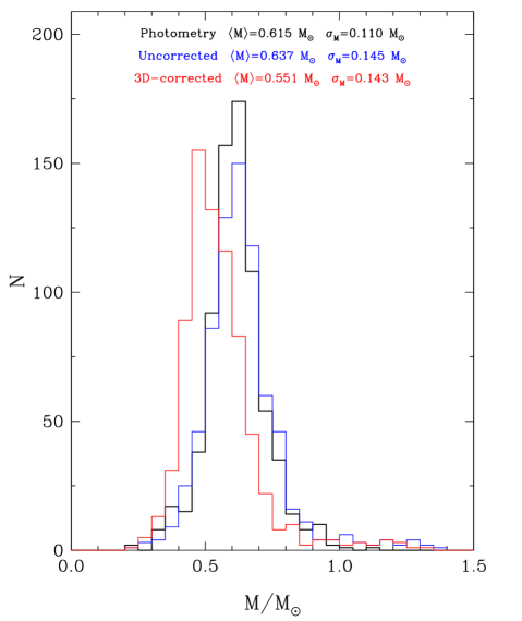
Figure 13: Relative mass distributions obtained from photometry (black) and spectroscopy (blue: uncorrected; red: 3D-corrected), for the DB white dwarfs in common between the photometric and spectroscopic samples. The objects with ${\rm S/N}<10$, $\sigma_{\pi}/\pi>0.25$, or marginal helium lines have been excluded. The mean masses and standard deviations are also given in the figure.

5.3 Hydrogen Abundance Distribution

The final parameter we need to discuss is the hydrogen abundance ratio, ${\rm H}/{\rm He}$, which is displayed in Figure 14 as a function of effective temperature for all the objects in our spectroscopic sample. Since the limit of detectability of H$\alpha$ depends on the quality of the spectroscopic observations, we only kept the spectrum with the highest S/N for the objects with multiple observations. Also, as mentioned above, we considered an object to be a DB star if only an upper limit on the hydrogen abundance could be determined by our fitting technique. With this definition, we find that 61% of the objects in our sample are DBA white dwarfs, a ratio which is similar to the 63% obtained by Rolland et al. (2018), but somewhat lower than the 75% reported by Koester & Kepler (2015), although their higher value was obtained by restricting their spectroscopic sample to ${\rm S/N}>40$ (their Table 3 actually reveals a much broader range of values).

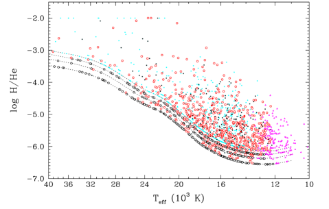
Figure 14: Hydrogen abundances as a function of effective temperature. The description of symbols is identical to that of Figure 7, with the exception that unresolved DB+DA candidates (see Section 6.1) are shown by red filled circles. Limits on the hydrogen abundance set by our spectroscopic observations at H$\alpha$ are shown as dotted lines for (from bottom to top) ${\rm S/N}>20$ (200 mÅ equivalent width), $15<{\rm S/N}<20$ (300 mÅ), $10<{\rm S/N}<15$ (400 mÅ), and ${\rm S/N}<10$ (500 mÅ).

The general abundance pattern observed in Figure 14 is consistent with the deepening of the helium convection zone as the star cools off (see, e.g., Figure 9 of Rolland et al. 2018), in which hydrogen is gradually being diluted into a larger and more massive convective envelope. It is thus not surprising to find some of the largest hydrogen abundances at high temperatures, where the helium convection zone is the shallowest. Note that in all cases, hydrogen always remains a trace element in the stellar envelope, and its presence does not affect the structure of the convection zone in any way (Rolland et al., 2018).

Despite the poor quality of some of the SDSS spectra with S/N < 10 (shown by cyan dots in Figure 14), we can see that the derived hydrogen abundances overlap perfectly with the bulk of our other determinations, except at the hot end of the sequence where H$\alpha$ becomes increasingly more difficult to detect, especially in low S/N spectra. In such cases our fitting algorithm may yield unreliable hydrogen abundance measurements. At the cool end of the sequence, however, we are able to obtain reasonable hydrogen abundances, even from white dwarf spectra where helium lines are barely detected.

Perhaps the most striking feature in Figure 14 is the range of H/He values at a given effective temperature, which can reach as much as 3 orders of magnitude near $T_{\rm eff}\sim 17,000$ K. Note that at these temperatures, H$\alpha$ can be easily detected spectroscopically, and hydrogen abundances as low as ${\rm H}/{\rm He}\sim 10^{-6}$ can be effectively measured, even with a relatively low S/N spectrum (see the detection limits in Figure 14). Even so, there is a significant fraction of DB white dwarfs in our sample, found at all temperatures, showing no H$\alpha$ absorption feature. Four of these, selected in a temperature range where H$\alpha$ can be most easily detected, are displayed in Figure 15. These cool DB stars have so little hydrogen that they must have maintained hydrogen-poor envelopes throughout their evolution. Hence, whatever scenario is invoked to explain the presence of hydrogen in DBA white dwarfs, it must be able to account for the large spread in hydrogen abundances observed here. We discuss this issue at length in Section 7.2.

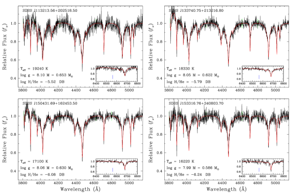
Figure 15: Best spectroscopic fit to four cool DB white dwarfs with no detectable H$\alpha$ feature. The best-fit model (red) is plotted over the normalized observed spectrum (black). The inset shows the region near H$\alpha$ (indicated by the tick mark) used to determine the hydrogen abundance, or upper limits. The derived atmospheric parameters are also given in each panel.

5.4 Comparison with Koester & Kepler (2015)

Koester & Kepler (2015) performed a similar analysis of the DB white dwarfs in the SDSS, also drawn from the SDSS DR10 and DR12. The comparison of their effective temperatures, surface gravities, and hydrogen abundances for the 996 objects in common with our analysis is presented in Figure 16. If we exclude the objects below $T_{\rm eff}=16,000$ K, for which Koester & Kepler assumed $\log g=8.0$, we find a good overall agreement between our atmospheric parameters and theirs. There are however some slight discrepancies between the two sets of values, in particular around $T_{\rm eff}\sim 24,000$ K where the helium lines reach their maximum strength. Around this region, our effective temperatures, surface gravities, and hydrogen abundances are in general higher than their values, but there is also a lot more scatter. Koester & Kepler also mention a deficiency of objects in the interval $T_{\rm eff}=24,000-26,000$ K (see their Figure 1 and Table 2), which they attribute to either the assumed convective efficiency, or to flux calibration issues with the SDSS spectra. While we use the same convective efficiency (ML2/$\alpha$=1.25) and the same SDSS spectra, we do not see such a depletion of objects in this temperature range (see, e.g., Figure 10). All these small discrepancies between their analysis and ours can probably be attributed to differences in model atmospheres and/or fitting techniques.

Figure 16: Differences in effective temperatures, surface gravities, and hydrogen abundances as a function of effective temperature between our analysis and that of Koester & Kepler (2015). The cyan dots represent the objects for which Koester & Kepler assumed $\log\textsl{{g}}=8.0$.

Koester & Kepler (2015) also find that, below $T_{\rm eff}\sim 16,000~{}{\rm K}$, their spectroscopic $\log\textsl{{g}}$ values (or masses) increase steadily, forming an almost continuous distribution (see their Figure 1). In particular, they find almost no cool DB white dwarfs with $\log\textsl{{g}}\sim 8.0$ in this temperature range, in contrast with our surface gravity distribution displayed in Figure 7, which shows a spread rather than a continuous increase in $\log\textsl{{g}}$ below $T_{\rm eff}\sim 16,000~{}{\rm K}$ (see also Figure 6 of Rolland et al. 2018). Moreover, we find a significant number of white dwarfs with normal masses (see Figure 8), or even lower than average. These discrepant results are most likely due to differences in the treatment of van der Waals broadening between both sets of model atmospheres. This may also explain the mean mass of 0.706 $M_{\odot}$ obtained by Koester & Kepler for their complete sample, while we find a much lower value of $0.63~{}M_{\odot}$.

5.5 Accuracy and Precision of the Fitting Techniques

At this point in our analysis, it is worth reevaluating the accuracy and the precision of both the photometric and spectroscopic techniques for determining the physical parameters of DB white dwarfs using the $ugriz$ photometry and optical spectra from the SDSS. In this context, the precision refers to the level of agreement of a measurement with itself when it is repeated several times, while the accuracy refers to the proximity of the measurement to the true physical value.

On the basis of our best data sets — i.e. the spectroscopic sample with ${\rm S/N}>10$ and the photometric sample with $\sigma_{\pi}/\pi<0.25$ — we conclude that, on average, the spectroscopic technique is more precise than the photometric technique for determining the effective temperatures of DB white dwarfs — $\langle\sigma_{T_{\rm eff}}\rangle=2.59\%$ from spectroscopy versus 8.72% from photometry — when using the SDSS photometric and spectroscopic data. At low effective temperatures, however, the photometric technique becomes as precise as the spectroscopic technique, if not more ($\langle\sigma_{T_{\rm eff}}\rangle\sim 2\%$ from photometry at 10,000 K). For the determination of stellar masses, the errors are also smaller from spectroscopy ($\langle\sigma_{M}\rangle=0.053~{}M_{\odot}$ from spectroscopy versus 0.112 $M_{\odot}$ from photometry). Of course, the photometric technique may potentially yield more precise mass measurements than the spectroscopic technique, regardless of the temperature range, provided that $\sigma_{\pi}/\pi$ is small enough (see section 4.1).

As mentioned in GBB19, the synthetic photometry is less affected by the input physics of the model atmospheres than the model spectra. For the DB white dwarfs analyzed here, the photometric mass distribution was found to be well centered on $M=0.6~{}M_{\odot}$, at all temperatures, while the spectroscopic distribution deviated from this value between 21,000 K and 17,000 K, as well as below 16,000 K (see Section 5.2). However, GBB19 found a good agreement between the photometric and spectroscopic temperatures, except at the hot end of the distribution, where the $ugriz$ photometry is in the Rayleigh-Jeans regime. We thus conclude that, for DB stars, both fitting techniques have a similar accuracy for the determination of effective temperatures, but the photometric technique is more accurate for measuring stellar masses.

Since we will compare in Section 7.1 the distribution of DB and DA white dwarfs, we briefly summarize some of the results from GBB19 regarding the DA stars. GBB19 found that the spectroscopic temperatures of DA stars were $\sim$10% higher than the photometric values for $T_{\rm eff}>14,000$ K, which they attributed to some inaccuracy in the theory of Stark broadening for hydrogen lines. The spectroscopic and photometric masses, however, were in very good agreement. We thus conclude that, for the DA stars, the photometric technique is more accurate than the spectroscopic technique for the determination of effective temperatures, but both techniques have a similar accuracy when it comes to mass determinations. As for the DB white dwarfs, GBB19 also found that the spectroscopic technique yields more precise temperature and mass measurements than the photometric technique.

6 Objects of Particular Astrophysical Interest

Our analysis of the atmospheric and physical parameters of DB white dwarfs, described in the previous section, has revealed the existence of several objects of particular astrophysical interest. We discuss these objects in turn.

6.1 Double Degenerate Candidates

Unresolved double degenerate binaries can be identified by their extremely low spectroscopic masses (see, e.g., Bergeron et al. 1992), or alternatively, by their overluminosities in Hertzsprung-Russel diagrams (see Figure 10 of Bergeron et al. 1997). In the last case, due to the presence of two stars in the system, the radius is overestimated, and thus the photometric mass is underestimated. GBB19 have already identified several such degenerate binaries in the SDSS data, both spectroscopically and photometrically.

One type of double degenerate system that can be easily recognized is those composed of a DA and a DB white dwarf, an excellent example of which is KUV 02196+2816, analyzed in detail by Limoges et al. (2009). The observed spectrum of such systems resembles that of a DBA white dwarf, but the hydrogen lines are usually extremely strong and poorly reproduced by single star, homogeneous models (see Figure 19 of GBB19). We identified a total of 10 DA+DB unresolved double degenerates in our sample, listed in Table 2. It is possible to obtain the effective temperatures of both components of the system by fitting the spectrum with a combination of pure hydrogen and helium-rich synthetic spectra. For simplicity, we assume here $\log\textsl{{g}}=8.0$ for both components of the system, and a pure helium atmosphere for the DB white dwarf. The photometric and spectroscopic solutions obtained for these systems under the assumption of a single star are reported in Table 2, together with the effective temperatures obtained for the individual DA and DB components; our best fits are also presented in Appendix A. Note that in all cases where a parallax measurement is available, the photometric $\log\textsl{{g}}$ values are significantly lower than those inferred from spectroscopy.

Of these 10 double degenerate systems, SDSS J150506.24+383017.39 has already been reported by GBB19, while SDSS J011356.38+301514.62 has been interpreted by Manseau et al. (2016) as a hot, chemically homogeneous DBA white dwarf with $T_{\rm eff}=29,200$ K, $\log\textsl{{g}}=7.91$, and $\log{\rm H}/{\rm He}=-1.05$. Our photometric solution for this last object, displayed in the top panel of Figure 17 and obtained under the assumption of a single star, implies a much lower temperature. Also, the low inferred photometric mass of only 0.236 $M_{\odot}$ clearly indicates the presence of a double degenerate system. In the lower panel, we compare the spectroscopic fit obtained by Manseau et al. (2016), our own spectroscopic solution at lower effective temperature, and our spectroscopic solution assuming a DA+DB system. Clearly, this last solution provides not only the best fit to the observed spectrum, but the average temperature of the system also agrees perfectly with the photometric temperature. Finally, SDSS J091016.43$+$210554.20 is classified as magnetic (Kleinman et al., 2013), but our fit displayed in Appendix A indicates that this is undoubtedly a DA+DB degenerate binary, and interestingly enough, both components appear to be magnetic! Indeed, Zeeman splitting can be easily detected in both hydrogen (H$\alpha$ in particular) and helium lines.

Table 2: List of DA+DB double degenerate candidates

	Photometry		Spectroscopy			Deconvolution
SDSS name	$T_{\rm eff}$	$M$	$T_{\rm eff}$	$M$	$\log{\rm H}/{\rm He}$	$T_{\rm DA}$	$T_{\rm DB}$
	(K)	($M_{\odot}$)	(K)	($M_{\odot}$)		(K)	(K)
011356.38+301514.62	14,030	0.24	16,780	0.69	$-$4.719	10,110	18,260
074419.82+302203.40	12,670	0.59	14,610	0.62	$-$5.270	11,330	15,770
084716.21+484220.40	15,280	0.62	14,680	0.88	$-$6.050	10,080	15,470
091016.43+210554.20	14,900	0.67	15,390	0.72	$-$5.745	9,580	15,610
101316.02+075915.20	18,880	0.32	18,870	0.73	$-$5.075	12,210	30,360
103609.48+193841.14	15,910	0.59	16,740	0.73	$-$4.509	9980	16,880
112711.72+325229.70	13,070	0.21	14,380	0.57	$-$5.532	10,410	15,260
113623.54+320403.80	15,590	0.59	18,370	0.82	$-$5.111	14,120	25,800
140615.80+562725.90	38,700	0.45	14,340	0.91	$-$5.512	13,360	48,810
150506.24+383017.39	12,620	0.30	14,110	0.39	$-$5.049	10,180	15,490

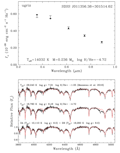
Figure 17: Top panel: Best photometric fit to SDSS J011356.38+301514.62 under the assumption of a single DBA white dwarf. Bottom panel: (top) best spectroscopic fit obtained by Manseau et al. (2016); (middle) our best spectroscopic fit at lower temperature; (bottom) our best fit obtained under the assumption of an unresolved DA+DB system. The atmospheric parameters of each fit are also given.

Another type of double degenerate system we found in our sample, also discussed in GBB19, is composed of two DB white dwarfs. Unlike the DA+DB systems, these DB+DB binaries cannot be easily recognized from spectroscopy alone, since the combination of two DB spectra resembles that of a single DB white dwarf with intermediate atmospheric parameters (see Figure 20 of GBB19). However, they can still be identified by comparing the spectroscopic and photometric masses since, as discussed above, unresolved double degenerate binaries will have low inferred photometric masses, but more normal spectroscopic masses. Because our mass estimates depend on the quality of the data, we restricted our photometric sample to objects with $\sigma_{\pi}/\pi<25\%$, and our spectroscopic sample to objects with ${\rm S/N}>10$; we also excluded spectra showing only marginal helium lines. We then flagged the objects for which $M_{\rm spec}-M_{\rm phot}\geq 0.2~{}M_{\odot}$. Similarly, we also flagged all objects with $M_{\rm phot}\leq 0.45~{}M_{\odot}$, because single star evolution predicts that such low-mass white dwarfs could not have formed within the lifetime of the Galaxy. After removing the previously identified DA+DB systems, we were left with 55 DB+DB unresolved double degenerate candidates. These systems, as well as the best photometric and spectroscopic solutions, are listed in Table 3. For the DA+DB systems, we were able to separate the contributions of each white dwarf. In the case of DB+DB binaries, it is possible, in principle, to deconvolve the parameters of both systems using the photometry and parallax information (Bédard et al., 2017), but this is clearly outside the scope of this paper. We would like to note that, since we applied a restriction on the quality of the trigonometric parallax as well as on ${\rm S/N}$, the list of DB+DB double degenerate systems given in Table 3 is by no means complete.

Table 3: List of DB+DB double degenerate candidates

	Photometry		Spectroscopy				Photometry		Spectroscopy
SDSS name	$T_{\rm eff}$	$M$	$T_{\rm eff}$	$M$	$\log{\rm H}/{\rm He}$	SDSS name	$T_{\rm eff}$	$M$	$T_{\rm eff}$	$M$	$\log{\rm H}/{\rm He}$
	(K)	($M_{\odot}$)	(K)	($M_{\odot}$)			(K)	($M_{\odot}$)	(K)	($M_{\odot}$)
000730.75+275111.90	13,932	0.41	16,305	0.63	$-5.880$	120203.13+285647.07	16,043	0.38	17,179	0.69	$-5.231$
002153.33+083141.82	27,313	0.49	17,789	0.81	$-5.733$	120735.19+225905.70	25,020	0.46	20,592	0.68	$-5.201$
004900.48-094203.00	18,466	0.46	19,419	0.78	$-4.434$	122444.73+174145.85	15,967	0.40	14,527	0.61	$-5.613$
010532.40+064234.18	13,368	0.36	13,404	0.41	$-5.694$	123230.41+035036.70	19,349	0.38	18,295	0.57	$-5.801$
011023.82+223716.25	12,275	0.42	12,771	0.59	$-5.714$	123735.52+602833.00	12,195	0.22	15,863	0.48	$-5.649$
011409.86+272739.42	15,833	0.34	17,540	0.68	$-4.887$	124058.65+532623.60	16,327	0.57	17,591	0.89	$-5.271$
020409.84+212948.58	15,071	0.59	20,605	0.83	$-3.186$	125030.21+594932.90	14,844	0.42	15,831	0.59	$-5.963$
024232.63-050954.75	12,181	0.40	14,438	0.56	$-5.871$	130106.26+023455.30	17,660	0.45	17,706	0.77	$-5.570$
034741.96+010823.80	26,320	0.55	17,809	0.78	$-4.844$	130830.53+470017.90	14,705	0.42	17,109	0.54	$-5.737$
052941.58+603806.80	13,612	0.39	16,823	0.50	$-5.665$	131658.16+305148.00	18,987	0.52	19,635	0.76	$-4.448$
064452.30+371144.30	14,077	0.41	15,241	0.57	$-6.030$	141337.74+450431.60	19,841	0.36	24,983	0.61	$-4.222$
075224.32+150352.34	12,219	0.38	13,562	0.54	$-6.373$	141621.79+322638.60	31,289	0.40	35,428	0.47	$-3.407$
082323.20+360834.79	14,876	0.39	15,180	0.65	$-6.208$	144650.87+285142.30	22,944	0.30	22,817	0.57	$-4.479$
083024.17+455206.02	15,272	0.45	14,546	0.57	$-5.296$	150301.95+053414.05	13,681	0.45	13,120	0.75	$-5.705$
093512.70+003857.12	12,472	0.36	12,853	0.60	$-6.053$	150647.60+310313.30	18,682	0.42	18,530	0.59	$-5.388$
093806.30+032242.53	20,190	0.49	18,864	0.74	$-5.068$	152320.96+005525.10	13,317	0.35	13,758	0.78	$-6.207$
094023.58+185837.24	12,891	0.33	13,449	0.53	$-6.219$	153024.23+331549.72	18,154	0.47	17,544	0.70	$-4.340$
094638.77+621759.50	12,248	0.40	12,840	0.34	$-6.244$	153316.76+340803.70	16,636	0.36	16,223	0.58	$-6.243$
095455.12+440330.30	18,398	0.59	23,829	0.79	$-4.416$	153735.17+063848.07	20,498	0.49	19,785	0.79	$-3.663$
100140.17+025853.19	16,397	0.52	18,526	0.73	$-4.689$	154811.34+083613.21	21,175	0.47	19,480	0.70	$-4.802$
100904.42+060817.50	18,565	0.45	18,325	0.83	$-5.384$	161735.37+311645.41	18,860	0.31	18,470	0.60	$-3.593$
101022.37+272239.30	17,118	0.38	16,028	0.59	$-6.085$	165339.17+174838.84	16,633	0.41	18,714	0.70	$-4.916$
101249.63+412311.04	15,888	0.52	16,363	0.89	$-5.260$	165946.51+393418.30	19,311	0.39	24,325	0.50	$-4.454$
102953.32+020812.45	14,963	0.39	14,201	0.70	$-4.853$	172243.19+603059.70	16,614	0.49	18,921	0.77	$-5.622$
103033.20+385447.59	21,194	0.44	20,387	0.80	$-4.810$	231041.15+141600.80	15,781	0.42	14,938	0.49	$-6.097$
104117.42+231036.40	25,880	0.42	21,596	0.63	$-4.784$	232344.88+150858.80	14,800	0.33	19,707	0.88	$-4.321$
105829.24+655227.20	13,665	0.43	15,381	0.42	$-6.182$	233305.10+005155.90	17,239	0.35	21,506	0.68	$-4.405$
111946.75+673631.10	13,284	0.39	15,207	0.60	$-5.625$

We summarize the results of this section by showing in Figure 18 the location of both DA+DB and DB+DB double degenerate candidates in a mass versus $T_{\rm eff}$ diagram. Remember that the photometric and spectroscopic temperatures generally differ for these systems. One can see that both types of binary systems are impossible to detect in spectroscopy alone, in contrast with the case of DA stars (see, e.g., Bergeron et al., 1992). However, most binary systems — but not all of them — appear as low-mass white dwarfs in the photometric mass distribution, even the DA+DB binaries.

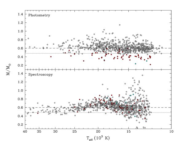
Figure 18: Photometric (top) and spectroscopic (bottom) masses as a function of effective temperature. DB+DB and DA+DB double degenerate candidates are shown as red and cyan circles, respectively. The horizontal dotted and dashed lines are located at $M=0.48~{}M_{\odot}$ and $M=0.6~{}M_{\odot}$, respectively.

6.2 DBA White Dwarfs with Large Hydrogen Abundances

There are several DBA white dwarfs in our sample with extremely large hydrogen abundances, defined arbitrarily here as $\log{\rm H}/{\rm He}>-3$. While we can find 9 such objects in Figure 14, only a single white dwarf with a very large hydrogen abundance ($\log{\rm H}/{\rm He}\sim-2$) has been identified by Rolland et al. (2018, see their Figure 5), namely PG 1311+129, also discussed at length by Bergeron et al. (2011). Among these 9 DBA stars in our sample, the five hottest objects above $T_{\rm eff}=24,000$ K have spectra with ${\rm S/N}\sim 10$ and the presence of H$\alpha$ cannot be confirmed with certainty. However, the four cooler DBA white dwarfs, displayed in Figure 19, have strong, and well-defined H$\alpha$ features. One of these objects is SDSS J153725.72+51526.90 (WD 1536+520), also analyzed in detail by Farihi et al. (2016). Our best spectroscopic fit yields a hydrogen abundance of $\log{\rm H}/{\rm He}=-2.16$, while Farihi et al. reported an even larger hydrogen abundance of $\log{\rm H}/{\rm He}=-1.70$, as well as large abundances of various heavy elements (O, Mg, Al, Si, Ca, Ti, Cr, Fe). Farihi et al. concluded that WD 1536+520 was currently accreting debris from a rocky and H₂O-rich parent body. The accretion of hydrogen in this process would also be responsible for the abnormally large hydrogen abundances observed in this DBA(Z) white dwarf. We discuss these objects further in Section 7.2.

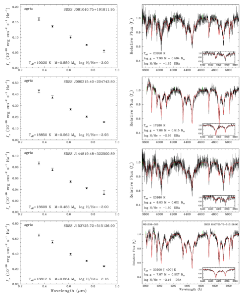
Figure 19: Best photometric (left) and spectroscopic (right) fits to four DBA white dwarfs in our sample with extremely large hydrogen abundances. The display is similar to that described in Figure 12.

6.3 DBZ White Dwarfs

We found a total of 118 white dwarfs in our sample with a published spectral type indicating the presence of metals (DBZ/DBAZ) in their spectrum. This is obviously a lower limit to the true number of DBZ stars, because the detection of metals — mostly the Ca ii H and K doublet — depends strongly on the spectral resolution and S/N. For instance, SDSS J153725.72+51526.90 (WD 1536+520), already displayed in Figure 19, shows large abundances of various heavy elements (O, Mg, Al, Si, Ca, Ti, Cr, Fe; Farihi et al. 2016), but it is classified as a DBA star in the SDSS. As discussed in Section 3, the DBZ white dwarfs in our sample have been fitted with a specific grid of model atmospheres that includes only calcium in the equation of state and opacity calculations. This is a simplistic approach, but at least it has the benefits of including the most important (probably only) metallic features detected in the SDSS spectra of DBZ white dwarfs.

We present in Figure 20 our best spectroscopic fits to four DBZ white dwarfs in our sample with strong Ca ii H and K lines, two of which also show a detectable H$\alpha$ absorption feature. In the other two cases, we detect no hydrogen, and its abundance is thus set to our limit of detectability ($\log{\rm H}/{\rm He}\ \lesssim-6$). Hence, even though the accretion of metals is often associated with the probable accretion of water-rich material (see Farihi et al. 2016, Gentile Fusillo et al. 2017, and references therein), giving rise to large photospheric hydrogen abundances such as in WD 1536+520, we do find in our sample some objects with large metal abundances, but with no detectable hydrogen in their atmospheres. This conclusion is based on DBZ white dwarfs found in a temperature range ($T_{\rm eff}\sim 14,000-17,000$ K) where our limit of detectability is extremely low (see Figure 14). We come back to this point below.

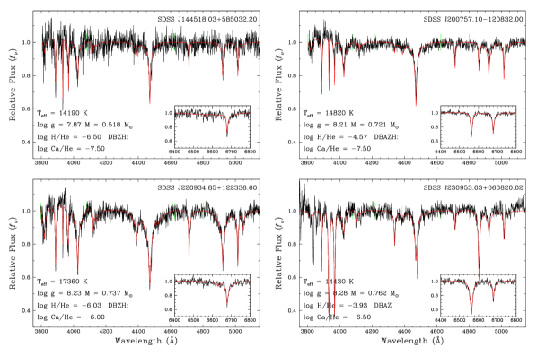
Figure 20: Best spectroscopic fits to four DBZ white dwarfs in our sample with strong Ca ii H & K lines, without (left) and with (right) detectable hydrogen features (H$\alpha$ region shown in the inset).

6.4 Magnetic White Dwarfs

In section 5.2, we discussed the presence of massive DB white dwarfs in our photometric sample. While most of these were found below $T_{\rm eff}\sim 22,000$ K, there are two very massive objects located around $T_{\rm eff}\sim 25,500$ K and 36,000 K (small black dots in the upper panel of Figure 10). These correspond to SDSS J094209.49+540157.50 and SDSS J143739.13+315248.80, which are classified as magnetic DB white dwarfs (DBH), with no clear absorption lines in their spectra, most likely due to the presence of a strong magnetic field. For both of these objects, the photometric fit yields a very large mass of $M\sim 1.3~{}M_{\odot}$. Even though our solutions for these objects are uncertain at best, magnetic white dwarfs do tend to be more massive than the non-magnetic population (Liebert, 1988; Ferrario et al., 2015), in agreement with our results.

In some other magnetic DB stars, the magnetic field is strong enough that Zeeman splitting of the helium lines becomes clearly visible. Three examples are presented in Figure 21, together with our fits to SDSS J094209.49+540157.50, mentioned in the previous paragraph. In the last case, our spectroscopic fit is meaningless because the spectrum is featureless, but the photometric fit appears reasonable. Note that most objects displayed here have large inferred photometric masses (including the featureless white dwarf at 1.344 $M_{\odot}$), but not all of them. Moreover, we also note in the case of the magnetic DA+DB double degenerate candidate SDSS J091016.43$+$210554.20, discussed above and displayed in Appendix A, that it has the highest inferred photometric mass in Table 2, which implies that both magnetic components of the system are also fairly massive.

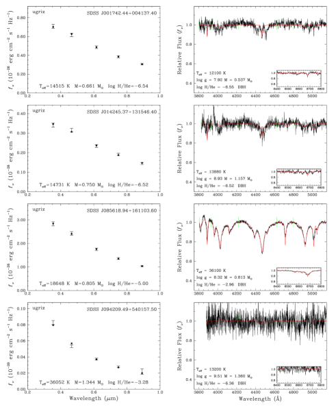
Figure 21: Best photometric (left) and spectroscopic (right) fits to four magnetic DB white dwarfs in our sample. The display is similar to that described in Figure 12.

7 Spectral Evolution of DB White Dwarfs

In the light of our results, we now focus our attention on the spectral evolution of DB white dwarfs. In particular, we discuss in turn the evolution of the DB-to-DA ratio as a function of effective temperature, and we revisit the question of the origin of hydrogen in DBA white dwarfs.

7.1 Evolution of the DB-to-DA Ratio

In order to determine the DB-to-DA ratio as a function of effective temperature, we retrieved the 27,216 spectra of DA white dwarfs identified in the SDSS DR7, DR10, and DR12 (Kleinman et al., 2013; Kepler et al., 2015, 2016). Since we want to characterize the entire population of DB and DA white dwarfs, we applied no criterion on the spectral type. Furthermore, to ensure the best possible determination of the atmospheric parameters for both DB and DA stars, we only kept the spectra with ${\rm S/N}>10$, and the best ${\rm S/N}$ spectrum for the objects with multiple observations. The model atmospheres and fitting technique used to obtain the atmospheric parameters for the DA stars are described at length in GBB19 and references therein.

Because the SDSS survey is magnitude limited, we need to take into account that DA and DB white dwarfs with similar $T_{\rm eff}$ and $\log\textsl{{g}}$ values have different absolute magnitudes (see, e.g., Figure 1 of Bergeron et al. 2019). Therefore, the volume sampled by each white dwarf type is different. To deal with this issue, we took advantage of the Gaia trigonometric parallaxes and retained only white dwarfs within 1 kpc. This left us with a sample of 9863 DA and 1145 DB white dwarfs. The composition of our sample, subdivided by spectral type, is presented in Table 4. We should note that the atmospheric parameters obtained for the irregular spectral types (magnetic, composite, etc.) are more uncertain, but this should not affect significantly our conclusions, since these subtypes represent only a small fraction of our total sample (see Table 4).

Table 4: Distribution of the different spectral subtypes in the DA and DB samples

DA sample			DB sample
Spectral Type	Number	Percentage	Spectral Type	Number	Percentage
DA	8440	85.57%	DB	859	75.02%
DAH	236	2.39%	DBH	12	1.05%
DAM/DA+M	725	7.35%	DBM/DB+M	41	3.58%
Other	99	1.00%	Other	2	0.17%
Uncertain	363	3.68%	Uncertain	231	20.47%
Total	9863	100%	Total	1145	100%

One important issue that also needs to be addressed is the spectroscopic completeness of the SDSS. One class of objects that was observed in this survey with a high priority is the so-called “hot standard” target class, which selects all isolated stars with clean photometry flags with very blue colors, $u-g<0$ and $g-r<0$, down to a flux limit of $g<19$ (Eisenstein et al., 2006b). Most DB white dwarfs satisfy this condition, as they only become redder below $T_{\rm eff}\sim 13,000~{}{\rm K}$ or so (see Figure 2 of Bergeron et al. 2019). However, in the case of DA white dwarfs, the $u-g<0$ criterion is only satisfied for $T_{\rm eff}\ \lower 2.15277pt\hbox{$\buildrel>\over{\sim}\ $}22,000~{}{\rm K}$. Eisenstein et al. (2006b) estimated that the completeness of the SDSS at $u-g>0$ is about 66% of that at $u-g<0$. Therefore, in the calculations presented below, we follow the same procedure as that described in Eisenstein et al. (2006a, see their Section 4), and increase the weight of the stars redder than $u-g=0$ by a factor of 1.5.

The distribution of DA and DB white dwarfs as a function of effective temperature is shown in Figure 22, using both spectroscopic and photometric temperatures. While there are small differences between the results obtained using these two temperature scales, the distributions show similar behaviors. In particular, the number of DB white dwarfs increases monotonically with decreasing effective temperature, before dropping again at lower temperatures when DB white dwarfs turn into DC stars, i.e. when neutral helium lines become barely detectable ($T_{\rm eff}\,\lesssim 12,000$ K).

More puzzling is the DA distribution, which shows a sudden drop around $T_{\rm eff}\sim 14,000~{}{\rm K}$ in spectroscopy, and around $T_{\rm eff}\sim 12,000~{}{\rm K}$ in photometry. The difference in the location of this local minimum can probably be explained in terms of small inaccuracies in our spectroscopic temperature scale. Indeed, this corresponds to the region where the Balmer lines reach their maximum strength, and our model spectra most likely predict stronger lines than what is actually observed, causing the spectroscopic solutions to be “pushed” on each side of the maximum (see also Figure 14 of Genest-Beaulieu & Bergeron 2014). Note that this may also be caused, in part, by residual calibration issues with the SDSS spectra, since the same experiment with the DA white dwarfs from the sample of Gianninas et al. (2011) showed an accumulation of objects instead of a depletion (see Figure 15 of Genest-Beaulieu & Bergeron 2014). But the fact remains that there is a sudden decrease of DA stars in this temperature range, regardless of the temperature scale (the increase in the number of DA stars at even cooler temperatures corresponds to the behavior expected from the white dwarf luminosity function). It is of course tempting to associate this drop with the onset of convective mixing at low effective temperature ($T_{\rm eff}\,\lesssim 12,000$ K; see Figure 16 of Rolland et al. 2018), which can transform DA white dwarfs into DC stars (or helium-rich DA stars with a very weak H$\alpha$ feature). But to confirm this hypothesis, one would have to include all non-DA white dwarfs in this particular range of temperature. Such a major endeavor is clearly outside the scope of this paper.

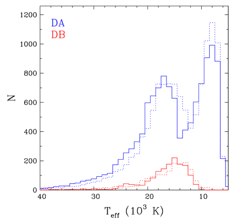
Figure 22: Number of DA and DB white dwarfs in our SDSS sample as a function of effective temperature. The solid and dotted distributions are based on spectroscopic and photometric temperatures, respectively. The objects with ${\rm S/N}<10$ and $D>1~{}{\rm kpc}$ have been excluded, and a weight factor of 1.5 has also been applied to the objects with $u-g>0$ (see text).

Of greater interest in the present context is the fraction of DB white dwarfs as a function of effective temperature, which we present in Figure 23. While we show here the results using spectroscopic temperatures, the results obtained from photometry are qualitatively similar. We also remind the reader that the two coolest temperature bins are not significant because DB white dwarfs turn into DC stars in this temperature range. Below $T_{\rm eff}=40,000~{}{\rm K}$, down to $\sim$27,000 K, the DB/(DA+DB) ratio remains fairly constant at $\sim$5%, within the uncertainties, and increases slowly to $\sim$7% near 20,000 K. Below this temperature, however, the DB/(DA+DB) ratio rapidly increases to a value of 25% near 15,000 K, until it drops again at lower temperatures when DB white dwarfs turn into DC stars. The picture depicted in Figure 23 is consistent with the results obtained by Bergeron et al. (2011), who determined the luminosity functions of DA and DB stars identified in the PG survey, and found that 20% of all white dwarfs below $T_{\rm eff}\sim 17,000$ K are DB stars (i.e. $M_{\rm bol}>9.5$ in their Figure 24), while at higher temperatures, only $\sim$$9$% of all white dwarfs are DB stars.

The variation of the DB/(DA+DB) ratio observed in Figure 23 is also entirely consistent with the convective dilution scenario, where the thin, radiative hydrogen layer present at the surface of hot DA white dwarfs is being convectively eroded by the deeper and more massive convective helium envelope, resulting in the conversion of a DA white dwarf into a DB star. Although detailed numerical simulations of this convective dilution process are still unavailable, an examination of the results displayed in Figures 9 and 10 of Rolland et al. (2018) reveals that objects with hydrogen layer masses in the range $\log M_{\rm H}/M_{\odot}=-15.5$ up to $-14$ would undergo a hydrogen- to helium-atmosphere transition between $T_{\rm eff}=30,000~{}{\rm K}$ and $18,000~{}{\rm K}$, respectively, in perfect agreement with the results obtained here (see also MacDonald & Vennes 1991). The fact that the DB/(DA+DB) ratio increases rather abruptly below 20,000 K also suggests a narrow range of hydrogen layer masses for the population of DA stars that undergo the DA-to-DB transition, somewhere in the order of $\log M_{\rm H}/M_{\odot}\sim-14$.

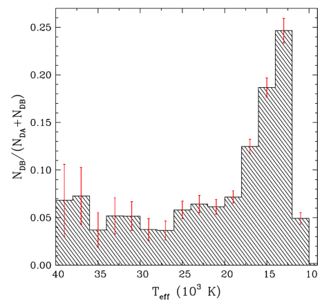
Figure 23: Ratio of the number of DB stars to the total number of DA+DB white dwarfs, as a function of (spectroscopic) effective temperature. The error bars represent the Poisson statistics of each bin. The objects with ${\rm S/N}<10$ and $D>1~{}{\rm kpc}$ have been excluded.

7.2 Origin of Hydrogen in DBA white dwarfs

Our hydrogen abundance determinations (or limits) from Figure 14 are reproduced in Figure 24 together with the detailed simulations from Rolland et al. (2018), which show the predictions of the convective dilution process, where a thin, superficial hydrogen layer of a given mass has been convectively diluted within the helium envelope, resulting in a homogeneously mixed H/He convection zone. More specifically, it is assumed in these calculations that the hydrogen layer has been convectively diluted, without paying attention to dilution process per say. These should thus not be interpreted as evolutionary sequences in any way. Each curve in Figure 24 represents the location of white dwarf stars with a constant value of $\log M_{\rm H}/M_{\odot}$, labeled in the figure. As discussed in Rolland et al., the sudden change of slope near $T_{\rm eff}\sim 20,000$ K corresponds to the temperature where the bottom of the helium convection zone sinks deep into the white dwarf, resulting in a further dilution of the photospheric hydrogen within the deeper helium reservoir as the star cools off.

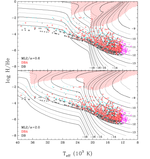
Figure 24: Predicted hydrogen abundances as a function of effective temperature (solid and dotted lines) from the simulations of Rolland et al. (2018) for homogeneously mixed models at 0.6 $M_{\odot}$ and for both the ML2/$\alpha=0.6$ (upper panel) and $\alpha=2$ (lower panel) versions of the mixing-length theory. Each curve is labeled with the corresponding value of $\log M_{\rm H}/M_{\odot}$. Results from Figure 14 are also reproduced. The red hatched areas represent the regions through which white dwarfs cannot evolve with a constant $\log M_{\rm H}/M_{\odot}$.

Also represented as red hatched areas in Figure 24 are regions in the $T_{\rm eff}$ – H/He parameter space through which white dwarfs cannot evolve continuously with a constant hydrogen mass (see Rolland et al. 2018 for a full discussion). Hence, in order for a white dwarf to cool off with a constant total mass of hydrogen already homogeneously mixed within the convective layer, it must be able to evolve continuously from the left to the right in this diagram along a single sequence with a given value of $\log M_{\rm H}/M_{\odot}$, without crossing this forbidden region. An examination of the results displayed in Figure 24 indicates that the hottest DBA white dwarfs in our sample ($T_{\rm eff}\gtrsim 20,000$ K) can be accounted for by this scenario if the total hydrogen mass is less than $\log M_{\rm H}/M_{\odot}\sim-15$, assuming the ML2/$\alpha=0.6$ parameterization of the mixing-length theory (or even less if convection is more efficient). Note also that in the smallest hydrogen mass models ($\log M_{\rm H}/M_{\odot}\lesssim-16$) at high temperatures, there is not enough hydrogen accumulated at the surface of the star to appear as a DA white dwarf (see Figures 3 and 4 of Manseau et al. 2016). In other words, the progenitors of some of the hottest DBA white dwarfs in our sample have never been genuine DA stars, and probably appeared as stratified DAB stars, with an extremely thin hydrogen layer floating in diffusive equilibrium at their surface. The hot ($T_{\rm eff}\sim 30,000$ K) DAB white dwarf SDSS J1509$-$0108, displayed in Figure 14 of Manseau et al. (2016), represents an excellent example of such a stratified white dwarf, with only $\log M_{\rm H}/M_{\star}=-16.78$ ($\log M_{\rm H}/M_{\odot}=\log M_{\rm H}/M_{\star}+0.22$ for a $M_{\star}\sim 0.6\ M_{\odot}$ white dwarf).

The other hot ($T_{\rm eff}>20,000$ K) DB white dwarfs in Figure 24 with no detectable traces of hydrogen have so little inferred total hydrogen mass in their stellar envelope that these stars always appeared as DB white dwarfs, and their immediate progenitors are most certainly the hot DB stars in the DB-gap analyzed by Eisenstein et al. (2006a). These obviously will remain DB stars, with no detectable traces of hydrogen, throughout their evolution. More importantly, even the hot DBA stars in our sample above $T_{\rm eff}\sim 20,000$ K await a similar fate, given that the deepening of the mixed H/He convection zone at lower temperatures will completely dilute any residual hydrogen left in the stellar envelope, well below the limit of visibility of hydrogen, H$\alpha$ in this case. In this respect, we disagree with the conclusions of Koester & Kepler (2015) who suggested that practically all DB white dwarfs probably show some trace of hydrogen if the spectroscopic resolution and S/N are high enough. Regardless of the observational limit, there is obviously also a theoretical limit on H/He, predicted by model atmospheres, below which hydrogen becomes invisible (see in particular Figure 3 of Rolland et al. 2018). Such threshold limits are certainly achieved according to the results displayed in Figure 24. Hence we conclude that, according to the convective dilution scenario alone, all hot ($T_{\rm eff}>20,000$ K) DB and DBA white dwarfs will most likely evolve into nearly pure helium-atmosphere white dwarfs at lower temperatures, with no detectable traces of hydrogen. In contrast, DBA stars at lower temperatures should retain a trace of hydrogen much longer since the depth of the mixed H/He convection zone remains almost constant below 20,000 K (see Figure 9 of Rolland et al. 2018), thus reducing any further dilution of hydrogen.

We now turn our attention to the bulk of DBA white dwarfs in our sample, found below $T_{\rm eff}\sim 20,000$ K in Figure 24. In order to account for the observed photospheric hydrogen abundances in these stars, the total hydrogen mass present in the stellar envelope must be in the range $-14<\log M_{\rm H}/M_{\odot}<-10$, regardless of the convective efficiency. The problem here is that hotter DA progenitors with such thick hydrogen layers in diffusive equilibrium at their surface — i.e. with chemically stratified envelopes — would inhibit convection in the deeper helium envelope (see Figure 11 of Rolland et al. 2018), preventing any DA-to-DB conversion in this temperature range. In DA white dwarfs with such thick hydrogen layers, mixing between the convective hydrogen layer and the deeper, and more massive helium envelope would eventually occur, but at much lower effective temperatures ($T_{\rm eff}\ \lesssim 12,000$ K) according to the calculations of Rolland et al. (2018, see their Figure 16). Hence we must conclude that the total amount of hydrogen present in the bulk of DBA white dwarfs below $T_{\rm eff}\sim 20,000$ K is too large to have a residual origin resulting from the convective dilution scenario, and that other sources of hydrogen must be invoked, such as accretion from the interstellar medium, comets, or disrupted asteroids, etc., a conclusion also reached in several previous investigations (e.g., MacDonald & Vennes 1991, Bergeron et al. 2011, Koester & Kepler 2015, Rolland et al. 2018). Despite these discrepancies, the convective dilution scenario remains the only viable explanation for the transformation of DA into DB white dwarfs below 20,000 K.

Finally, we note that all the DBA white dwarfs in our sample completely avoid the so-called forbidden region in Figure 24 (defined by the red hatched areas), especially with the ML2/$\alpha=0.6$ models. Note, in particular, how the most hydrogen-rich DBA stars in our sample (including PG 1311+129), already discussed in Section 6.2, follow nicely the bottom limit of the forbidden region. Because the convective dilution process, which transforms a chemically stratified DA star into a homogeneous DB white dwarf, makes somehow the object “jump” over this forbidden region, the extreme DBA stars in our sample are probably in the process of being convectively mixed, with hydrogen constantly trying to float back to the surface, as suggested by Bergeron et al. (2011) in the case of PG 1311+129, which incidentally, shows small spectroscopic variations as a function of time (see their Figure 28).

8 Discussion

We presented a detailed model atmosphere analysis of DB white dwarfs drawn from the SDSS database. The large set of optical spectra and $ugriz$ photometry available from the SDSS, coupled with the exquisite trigonometric parallax measurements from the Gaia mission, allowed us to measure the fundamental parameters of DB white dwarfs using both the spectroscopic and photometric techniques. In turn, the results obtained from both fitting techniques provided us with a unique opportunity to assess the precision, but more importantly the accuracy of the measurements, in particular the effective temperature, stellar mass, and photospheric composition, which form the basic elements for understanding the origin and evolution of these stars.

We identified several problems in our analysis, both theoretical and observational. On the theoretical front, van der Waals broadening remains the largest source of uncertainty in the calculations of synthetic spectra for DB white dwarfs. Nevertheless, our mass comparison displayed in Figure 10 reveals that the spectroscopic masses at low temperatures appear fairly reasonable, if we exclude the objects with extremely weak helium lines. We also see some clear evidence for 3D hydrodynamical effects in our spectroscopic mass distributions in the $16,000-22,000$ K temperature range, and additional work along the lines of Cukanovaite et al. (2018), but by including traces of hydrogen, should improve the spectroscopic mass measurements significantly. Finally, given the large spectroscopic data set available here, it would probably be worth revisiting the question of the convective efficiency in hot DB stars — which in all recent investigations, including ours, has been set to ML2/$\alpha=1.25$ — by repeating the experiments performed in Section 4.4 of Bergeron et al. (2011).

We identified a few problems on the observational front as well. While the number of white dwarfs discovered by the SDSS has been increased by more than a factor of 10 since the latest version of the Villanova White Dwarf Catalog of McCook & Sion (1999), the optical spectra from the SDSS still appear to suffer from some residual flux calibration problems. This becomes apparent at high effective temperatures, where the spectroscopic masses are lower than those measured at cooler temperatures, or lower than those inferred from photometry for that matter. This problem is observed for both DA and DB stars. Furthermore, even though the large number of white dwarf spectra available in the SDSS has significantly improved our understanding of these objects, the generally low S/N of the SDSS spectra (see Figure 1) still represents a strong limitation in terms of making more precise spectroscopic measurements of white dwarf parameters, and it is hoped that future spectroscopic surveys will improve the situation.

Our analysis has uncovered several interesting objects, including the existence of massive DB white dwarfs, mostly below $T_{\rm eff}\sim 18,000$ K, whose progenitor might be the Hot DQ stars. We also identified a large population of unresolved double degenerate binaries composed of two DB white dwarfs, and even occasionally DB+DA double degenerates. As in previous investigations, we did not find any evidence for single low-mass ($M<0.48\ M_{\odot}$) DB white dwarfs, obviously because nature does not produce such objects. All low-mass white dwarfs appear to have hydrogen-rich atmospheres. As discussed by Bergeron et al. (2011), common envelope evolution is required to produce such low mass white dwarfs, and this close-binary evolutionary channel must produce white dwarfs with hydrogen layers too massive to allow the DA to DB conversion at any temperature.

Probably the most important key result of our analysis is the hydrogen abundance (or limits) distribution as a function of effective temperature, summarized in Figure 24. This picture represents a static view, or a snapshot in time, of the current distribution of hydrogen abundances in DB and DBA white dwarfs, which detailed evolutionary calculations must eventually explain. In particular, DA white dwarfs must be able to turn into DB stars in the appropriate temperature range, and properly account for the observed DB-to-DA ratio. The residual amount of hydrogen expected from the DA-to-DB transition is much smaller than that inferred from current homogeneous envelope models (Rolland et al., 2018), unless the hydrogen-to-helium abundance ratio measured using homogeneous model atmospheres is somehow overestimated, for instance, if the atmosphere is chemically inhomogeneous (MacDonald & Vennes 1991, Genest-Beaulieu & Bergeron 2017). The alternative is to have an external source of hydrogen — either from the interstellar medium, disrupted asteroids, small planets, or even comets — polluting the atmosphere of DB white dwarfs after the DA-to-DB transition has occurred.

Yet, another alternative proposed by B. Rolland et al. (2019, in preparation) is to have an internal source of hydrogen. With this new paradigm, hydrogen is initially diluted in the deep stellar envelope of a hot PG1159 progenitor. With time, hydrogen slowly diffuses upward, slowly building a superficial hydrogen-rich atmosphere. However, calculations show that when the convective dilution process occurs, the resulting abundance profile is far from equilibrium, and large amounts of hydrogen are still present in the deep interior. As the convection zone of the cooling DB stars grows, large amounts of hydrogen is being dredged-up to the surface, a phenomenon similar to that invoked in the context of DQ white dwarfs (Pelletier et al., 1986).

Also of importance in this context is the existence, and persistence, of pure DB stars, i.e. helium-atmosphere white dwarfs that show no hydrogen feature whatsoever. As discussed in our analysis, this is not a simple problem of detectability, because envelope models such as those displayed in Figure 24 do predict hydrogen abundances where H$\alpha$ simply becomes undetectable, even theoretically. White dwarfs with such small total amounts of hydrogen present in their envelope — in particular those discovered in the DB gap — can only be explained by the so-called born-again post-AGB (asymptotic giant branch) evolutionary scenario, involving a very late helium-shell flash, or an AGB final thermal pulse, as described in detail by Werner & Herwig (2006). As discussed in Bergeron et al. (2019), it is possible that in this process, the total mass of helium could also be significantly reduced. This could perhaps explain the origin of cool DQ white dwarfs, in which carbon is being dredged-up from the core, a process that occurs only if the helium envelope is not too thick according to Pelletier et al. (1986). If this interpretation is correct, the immediate progenitors of DQ stars could be the “pure” DB white dwarfs discussed above. By the same token, one could imagine that these very late helium-shell flashes are violent enough as to wipe out the stellar environment from any planetary debris, thus providing a natural explanation for the absence of metals in cool DQ stars.

Clearly, all these issues will require larger and better data sets — higher S/N spectra in particular — but most importantly, state-of-the-art evolutionary model calculations able to predict the spectral evolution of white dwarf stars as a function of their cooling age. Then perhaps one day, we will be able to map the range of total hydrogen mass ($M_{\rm H}$) present in these stars — arguably the Holy Grail of white dwarf astrophysics.

We are grateful to Patrick Tremblay for useful discussions regarding the behavior of DB model spectra. This work is supported in part by the NSERC Canada and by the Fund FRQ-NT (Québec).

Appendix A DA+DB unresolved double degenerate systems

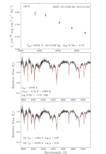
Figure 25: SDSS J011356.38+301514.62. The complete figure set (10 images) is available in the online journal.

References

- Abazajian et al. (2003) Abazajian, K., Adelman-McCarthy, J. K., Agüeros, M. A., et al. 2003, AJ, 126, 2081
- Beauchamp et al. (1996) Beauchamp, A., Wesemael, F., Bergeron, P., Liebert, J., & Saffer, R. A. 1996, in Astronomical Society of the Pacific Conference Series, Vol. 96, Hydrogen Deficient Stars, ed. C. S. Jeffery & U. Heber, 295
- Bédard et al. (2017) Bédard, A., Bergeron, P., & Fontaine, G. 2017, ApJ, 848, 11
- Bergeron et al. (2019) Bergeron, P., Dufour, P., Fontaine, G., et al. 2019, arXiv e-prints, arXiv:1904.02022
- Bergeron et al. (1997) Bergeron, P., Ruiz, M. T., & Leggett, S. K. 1997, ApJS, 108, 339
- Bergeron et al. (1992) Bergeron, P., Saffer, R. A., & Liebert, J. 1992, ApJ, 394, 228
- Bergeron et al. (2011) Bergeron, P., Wesemael, F., Dufour, P., et al. 2011, ApJ, 737, 28
- Cukanovaite et al. (2018) Cukanovaite, E., Tremblay, P. E., Freytag, B., Ludwig, H. G., & Bergeron, P. 2018, MNRAS, 481, 1522
- Deridder & van Rensbergen (1976) Deridder, G., & van Rensbergen, W. 1976, A&AS, 23, 147
- Dufour et al. (2008) Dufour, P., Fontaine, G., Liebert, J., Schmidt, G. D., & Behara, N. 2008, ApJ, 683, 978
- Dufour et al. (2007) Dufour, P., Liebert, J., Fontaine, G., & Behara, N. 2007, Nature, 450, 522
- Dunlap & Clemens (2015) Dunlap, B. H., & Clemens, J. C. 2015, in Astronomical Society of the Pacific Conference Series, Vol. 493, 19th European Workshop on White Dwarfs, ed. P. Dufour, P. Bergeron, & G. Fontaine, 547
- Eisenstein et al. (2006a) Eisenstein, D. J., Liebert, J., Koester, D., et al. 2006a, AJ, 132, 676
- Eisenstein et al. (2006b) Eisenstein, D. J., Liebert, J., Harris, H. C., et al. 2006b, ApJS, 167, 40
- El-Badry et al. (2018) El-Badry, K., Rix, H.-W., & Weisz, D. R. 2018, ApJ, 860, L17
- Farihi et al. (2016) Farihi, J., Koester, D., Zuckerman, B., et al. 2016, MNRAS, 463, 3186
- Ferrario et al. (2015) Ferrario, L., de Martino, D., & Gänsicke, B. T. 2015, Space Sci. Rev., 191, 111
- Fontaine et al. (2001) Fontaine, G., Brassard, P., & Bergeron, P. 2001, PASP, 113, 409
- Fontaine & Wesemael (1987) Fontaine, G., & Wesemael, F. 1987, in IAU Colloq. 95: Second Conference on Faint Blue Stars, ed. A. G. D. Philip, D. S. Hayes, & J. W. Liebert, 319–326
- Gaia Collaboration et al. (2018) Gaia Collaboration, Brown, A. G. A., Vallenari, A., et al. 2018, A&A, 616, A1
- Genest-Beaulieu & Bergeron (2014) Genest-Beaulieu, C., & Bergeron, P. 2014, ApJ, 796, 128
- Genest-Beaulieu & Bergeron (2017) Genest-Beaulieu, C., & Bergeron, P. 2017, in 20th European White Dwarf Workshop, ed. P. E. Tremblay, B. Gaensicke, & T. Marsh, Vol. 509, 201
- Genest-Beaulieu & Bergeron (2019) —. 2019, ApJ, 871, 169
- Gentile Fusillo et al. (2017) Gentile Fusillo, N. P., Gänsicke, B. T., Farihi, J., et al. 2017, MNRAS, 468, 971
- Gentile Fusillo et al. (2019) Gentile Fusillo, N. P., Tremblay, P.-E., Gänsicke, B. T., et al. 2019, MNRAS, 482, 4570
- Gianninas et al. (2011) Gianninas, A., Bergeron, P., & Ruiz, M. T. 2011, ApJ, 743, 138
- Harris et al. (2006) Harris, H. C., Munn, J. A., Kilic, M., et al. 2006, AJ, 131, 571
- Iben (1990) Iben, Jr., I. 1990, ApJ, 353, 215
- Kepler et al. (2015) Kepler, S. O., Pelisoli, I., Koester, D., et al. 2015, MNRAS, 446, 4078
- Kepler et al. (2016) —. 2016, MNRAS, 455, 3413
- Kilic et al. (2018) Kilic, M., Hambly, N. C., Bergeron, P., Genest-Beaulieu, C., & Rowell, N. 2018, MNRAS, 479, L113
- Kleinman et al. (2013) Kleinman, S. J., Kepler, S. O., Koester, D., et al. 2013, ApJS, 204, 5
- Koester & Kepler (2015) Koester, D., & Kepler, S. O. 2015, A&A, 583, A86
- Koester et al. (2009) Koester, D., Voss, B., Napiwotzki, R., et al. 2009, A&A, 505, 441
- Liebert (1988) Liebert, J. 1988, Publications of the Astronomical Society of the Pacific, 100, 1302
- Liebert et al. (2005) Liebert, J., Bergeron, P., & Holberg, J. B. 2005, ApJS, 156, 47
- Liebert et al. (1986) Liebert, J., Wesemael, F., Hansen, C. J., et al. 1986, ApJ, 309, 241
- Limoges & Bergeron (2010) Limoges, M.-M., & Bergeron, P. 2010, ApJ, 714, 1037
- Limoges et al. (2009) Limoges, M. M., Bergeron, P., & Dufour, P. 2009, ApJ, 696, 1461
- MacDonald & Vennes (1991) MacDonald, J., & Vennes, S. 1991, ApJ, 371, 719
- Manseau et al. (2016) Manseau, P. M., Bergeron, P., & Green, E. M. 2016, ApJ, 833, 127
- McCook & Sion (1999) McCook, G. P., & Sion, E. M. 1999, The Astrophysical Journal Supplement Series, 121, 1
- Pelletier et al. (1986) Pelletier, C., Fontaine, G., Wesemael, F., Michaud, G., & Wegner, G. 1986, ApJ, 307, 242
- Raddi et al. (2015) Raddi, R., Gänsicke, B. T., Koester, D., et al. 2015, MNRAS, 450, 2083
- Rolland et al. (2018) Rolland, B., Bergeron, P., & Fontaine, G. 2018, ApJ, 857, 56
- Tremblay et al. (2011) Tremblay, P.-E., Bergeron, P., & Gianninas, A. 2011, ApJ, 730, 128
- Tremblay et al. (2019) Tremblay, P. E., Cukanovaite, E., Gentile Fusillo, N. P., Cunningham, T., & Hollands, M. A. 2019, MNRAS, 482, 5222
- Tremblay et al. (2013a) Tremblay, P.-E., Ludwig, H.-G., Steffen, M., & Freytag, B. 2013a, A&A, 552, A13
- Tremblay et al. (2013b) —. 2013b, A&A, 559, A104
- Unsold (1955) Unsold, A. 1955, Physik der Sternatmospharen, MIT besonderer Berucksichtigung der Sonne.
- Veras et al. (2014) Veras, D., Shannon, A., & Gänsicke, B. T. 2014, MNRAS, 445, 4175
- Voss et al. (2007) Voss, B., Koester, D., Napiwotzki, R., Christlieb, N., & Reimers, D. 2007, A&A, 470, 1079
- Werner & Herwig (2006) Werner, K., & Herwig, F. 2006, PASP, 118, 183