Portable simulation framework for diffusion MRI

Abstract

The numerical simulation of the diffusion MRI signal arising from complex tissue micro-structures is helpful for understanding and interpreting imaging data as well as for designing and optimizing MRI sequences. The discretization of the Bloch-Torrey equation by finite elements is a more recently developed approach for this purpose, in contrast to random walk simulations, which has a longer history. While finite elements discretization is more difficult to implement than random walk simulations, the approach benefits from a long history of theoretical and numerical developments by the mathematical and engineering communities. In particular, software packages for the automated solutions of partial differential equations using finite elements discretization, such as FEniCS, are undergoing active support and development. However, because diffusion MRI simulation is a relatively new application area, there is still a gap between the simulation needs of the MRI community and the available tools provided by finite elements software packages. In this paper, we address two potential difficulties in using FEniCS for diffusion MRI simulation. First, we simplified software installation by the use of FEniCS containers that are completely portable across multiple platforms. Second, we provide a portable simulation framework based on Python and whose code is open source. This simulation framework can be seamlessly integrated with cloud computing resources such as Google Colaboratory notebooks working on a web browser or with Google Cloud Platform with MPI parallelization. We show examples illustrating the accuracy, the computational times, and parallel computing capabilities. The framework contributes to reproducible science and open-source software in computational diffusion MRI with the hope that it will help to speed up method developments and stimulate research collaborations.

,

1 Introduction

The numerical simulation of the diffusion MRI signal arising from complex tissue micro-structures is helpful for understanding and interpreting imaging data as well as for designing and optimizing MRI sequences.

It can be classified into two main groups. The first group is referred to as Monte-Carlo simulations in the literature and previous works include [1, 2, 3, 4, 5]. Software packages include the UCL Camino Diffusion MRI Toolkit [6], which has been widely used in the field. The second group of simulations relies on solving the Bloch-Torrey PDE in a geometrical domain, either using finite difference methods (FDM) [7, 8, 9, 10], typically on a Cartesian grid, or finite element methods (FEM), typically on a tetrahedral grid. Previous works on FEM include [11] for the short gradient pulse limit of some simple geometries, [12] for the multi-compartment Bloch-Torrey equation with general gradient pulses, and [13] with the flow and relaxation terms added. In [14], a simplified 1D manifold Bloch-Torrey equation was solved to study the diffusion MRI signal from neuronal dendrite trees. FEM in a high-performance computing framework was proposed in [15, 16] for diffusion MRI simulations on supercomputers. An efficient simulation method for thin media was proposed in [17]. A comparison of the Monte-Carlo approach with the FEM approach for the short pulse limit was performed in [11], where FEM simulations were evaluated to be more accurate and faster than the equivalent modeling with Monte-Carlo simulations. Recently, SpinDoctor, a Matlab-based diffusion MRI simulation toolbox that discretizes the Bloch-Torrey equation using finite elements, was released [18] and shown to be faster than Monte-Carlo based simulations for other diffusion sequences.

The discretization of the Bloch-Torrey equation by finite elements is a more recently developed approach for the purpose of dMRI simulations, in contrast to random walk simulations, which have a longer history. While finite element discretization is more difficult to implement than random walk simulations, the approach benefits from from long-established theoretical and numerical developments by the mathematical and engineering communities. In particular, software packages for the automated solutions of partial differential equations using finite element discretization, such as FEniCS [19, 20], are subject to active support and development. However, because diffusion MRI simulation is a relatively new application area, there is still a gap between the simulation needs of the MRI community and the available tools built on top of these finite elements software packages.

The deployment of FEniCS containers [21] opens a new direction to improve productivity and sharing in the scientific computing community. In particular, it can dramatically improve the accessibility and usability of high-performance computing (HPC) systems. In this paper, we address two potential difficulties in using FEniCS for diffusion MRI simulation. First, we simplified software installation by the use of FEniCS containers that are completely portable across multiple platforms. Second, we provide a simulation framework written in Python and whose code is open source. This simulation framework can be seamlessly integrated with cloud computing resources such as Google Colaboratory notebooks (working on a web browser) or with Google Cloud Platform with MPI parallelization.

One of the advantages of the simulation framework we propose here over the Matlab-based SpinDoctor [18] is that the Python code is free, whereas SpinDoctor requires the purchase of the software Matlab. Many researchers are now adopting Python since it is a free, cross-platform, general-purpose and high-level programming language. Plenty of Python scientific packages are available with extensive documentation such as SciPy for fundamentals of scientific computing, NumPy for large and multi-dimensional arrays and matrices, SymPy for symbolic computation, IPython for the enhanced interactive console, Pandas for data structures & analysis, Matplotlib for comprehensive 2D plotting. In addition, parallel computing for finite elements is relatively easy to implement within FEniCS, thus, this framework has advantages over SpinDoctor for very large scale problems.

The disadvantage of this simulation framework compared to SpinDoctor is the current lack of high-order adaptive time-stepping methods in Python tailored to the kind of ODEs systems coming from finite elements discretization, whereas such time-stepping methods are available in Matlab. Thus, in contrast to SpinDoctor where an adaptive, variable order, time-stepping method is used, the time-stepping method in the proposed framework is the $\theta-$method, with a fixed time step size. The $\theta-$method can be second-order accurate if $\theta$ is chosen to be $\frac{1}{2}$.

The simulation framework we propose can meet the following simulation needs:

1. the specification of an intrinsic diffusion tensor and a $T_{2}-$relaxation coefficient in each geometrical compartment;

2. the specification of a permeability coefficient on the interface between the geometrical compartments;

3. the periodic extension of the computational domain (assumed a box);

4. the specification of general diffusion-encoding gradient pulse sequences;

5. the simulation of thin-layer and thin-tube media using a discretization on manifolds;

Since this framework is based on FEniCS, packaged as an image, it inherits all functionalities of FEniCS related to mesh generation, mesh adaptivity, finite elements matrices construction, linear system solve, solution post-processing and display, as well as the underlying FEniCS computational optimization related to the above tasks. Finally, the framework is conceived with cloud computing and high performance computing in mind, thus, it

1. supports Cloud Computing with Google Colaboratory and Google Cloud Platform;

2. allows for MPI parallelization.

The paper is organized as follows. In Section 2 we recall the diffusion MRI simulation model based on the Bloch-Torrey equation. Then, we propose a portable simulation framework in Section 3 for which the numerical validation and the comparison are carried out in Section 4. Several simulations examples are shown in Section 5. We share some perspectives about the proposed framework in Section 6. The paper is finalised with a conclusion in Section 7.

2 Theory

The evolution of the complex transverse magnetization $U(\bm{x},t)$ over time $t$ can be described by the Bloch-Torrey equation [22]. For simplicity we consider a medium composed of two compartments, $\Omega=\Omega_{0}\cup\Omega_{1}$, each of which may be disconnected (see Fig. 1a). The equation takes the following form

$$\frac{\partial U(\bm{x},t)}{\partial t}=-i\,\gamma f(t)\,\bm{g}\cdot\bm{x}\,U(\bm{x},t)-\frac{U(\bm{x},t)}{T_{2}(\bm{x})}+\nabla\cdot\Bigl{(}\bm{D}(\bm{x})\,\nabla U(\bm{x},t)\Bigl{)}$$ (1)

where $i$ is the complex unit ($i^{2}=-1$), $\gamma=2.67513\times 10^{8}\,\rm rad\,s^{-1}T^{-1}$ is the gyromagnetic ratio of the water proton, and $\bm{g}$ is the diffusion gradient including gradient strength $g=\|\bm{g}\|$ and gradient direction $\bm{q}=\frac{\bm{g}}{\|\bm{g}\|}$. In the general case, ${\bm{D}}(\bm{x})$ is the diffusion tensor, a symmetric positive definite $3\times 3$ matrix. $T_{2}$ relaxation is the process by which the transverse magnetization decays or dephases.

On the interfaces between different compartments the magnetization is allowed to be discontinuous via the use of a permeability coefficient $\kappa$ [23]

$$\Bigl{\llbracket}\bm{D}\,\nabla U\cdot\bm{n}^{0}\Bigl{\rrbracket} =0$$ (2)

$$\Bigl{\{}\bm{D}\,\nabla\,U\cdot\bm{n}^{0}\Bigl{\}} =-\kappa\,\llbracket U\rrbracket$$

for $\bm{x}\in\Gamma=\partial\Omega_{0}\cap\partial\Omega_{1}$ and $\bm{n}^{k}$ is a normal vector pointing outward $\Omega_{k}$.

(a)

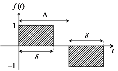
(b)

Figure 1: A composed domain $\Omega=\Omega_{0}\cup\Omega_{1}$ (a), and a PGSE sequence (b).

The temporal profile $f(t)$ can vary for different applications and the most commonly used diffusion-encoding sequence in diffusion MRI literature is called the Pulsed-Gradient Spin Echo (PGSE) sequence [24]. For this sequence, one can write $f(t)$ in the following way (see also Fig. 1b):

$$f(t)=\begin{cases}1,\quad&0\leq t\leq\delta,\\ -1,\quad&\Delta<t\leq\Delta+\delta,\\ 0,\quad&\text{otherwise.}\end{cases}$$ (3)

The quantity $\delta$ is the duration of the diffusion-encoding gradient pulse and $\Delta$ is the time delay between the start of the two pulses. Beyond the PGSE, the Oscillating Gradient Spin Echo (OGSE) [25], nonstandard diffusion sequences such as double diffusion encoding [26, 27, 28, 29] and multidimensional diffusion encoding [30] can be modelled.

Concerning the boundary conditions (BCs) on the exterior boundaries $\partial\Omega$, there are two options that are very often employed. One is placing the spins to be simulated sufficiently away from $\partial\Omega$ and impose simple BCs on $\partial\Omega$ such as homogeneous Neumann conditions. This supposes that the spins would have a low probability of having arrived at $\partial\Omega$ during the diffusion experiment. Another option is to place the spins anywhere desired, but to assume that $\Omega$ is repeated periodically in all space directions to fill $\mathbb{R}^{d}$, for example, $\Omega=\prod_{k=1}^{d}[a_{k},b_{k}]$. So, one can mimic the phenomenon where the water molecules can enter and exit the computational domain. Under this assumption of periodic continuation of the geometry, the magnetization satisfies pseudo-periodic BCs on $\partial\Omega$ [8]

$$U_{m} =U_{s}e^{{i\,\theta_{k}(t)}},$$ (4)

$$\bm{D}_{m}\,\nabla U_{m}\cdot\bm{n} =\bm{D}_{s}\,\nabla U_{s}\cdot\bm{n}\,e^{{i\,\theta_{k}(t)}},$$

where

$$U_{m}=\left.U(\bm{x},t)\right|_{x_{k}=a_{k}},\quad U_{s}=\left.U(\bm{x},t)\right|_{x_{k}=b_{k}}$$

$$\nabla U_{m}\cdot\bm{n}=\nabla U(\bm{x},t)\cdot\bm{n}\,\biggl{|}_{x_{k}=a_{k}},\quad\nabla U_{s}\cdot\bm{n}=\nabla U(\bm{x},t)\cdot\bm{n}\,\biggl{|}_{x_{k}=b_{k}}$$

and

$$\theta_{k}(t):=\gamma\;g_{k}\,(b_{k}-a_{k})\,\mathcal{F}(t),k=1,\cdots,d,\quad\mathcal{F}(t)=\int\limits_{0}^{t}f(s)\,ds.$$

Here we use ‘m’ and ‘s’ to indicate master and slave components of the pseudo-periodic BCs. The master-slave method corresponds to the implementation of the periodic BCs [31].

The MRI signal $S$ is the total transverse magnetization $U(\bm{x},t)$ over $\Omega$ measured at the echo time $T$

$$S=\int_{\bm{x}\in\Omega}U(\bm{x},T)\;d\bm{x}$$ (5)

The signal is usually plotted against the gradient strength $g=\|\mathbf{g}\|$ or a quantity called the $b$-value which is defined as the following

$$b=\gamma^{2}\|\mathbf{g}\|^{2}\int\limits_{0}^{T}{\mathcal{F}(s)^{2}}\,ds.$$ (6)

3 Method

For software portability, we consider two container technologies which are Docker [32] and Singularity [33]. They allow for bundling the whole collection of software packages that a user needs in a single file, that can be shared and used by collaborators. This would make a huge impact in scientific applications, where reproducibility is a core concern [34]. In particular, this enables us to develop software that other users can easily test. A software update reduces to a matter of downloading the newest version of a single file and different versions can coexist next to each other for easy consistency checks. We choose Docker for the IPython notebooks and Singularity for the deployment on HPC infrastructure. They follow the same workflow as the following

3.1 Diffusion MRI simulation library

The solution of the Bloch-Torrey equation and other functionalities related to diffusion MRI simulations have been packaged into Python library DmriFemLib, saved in GitHub.

https://github.com/van-dang/DMRI-FEM-Cloud/blob/master/DmriFemLib.py

Due to considerations related to the way FEniCS envisions the PDE solution workflow, and the fact that the PDE from the diffusion MRI simulation problem has some important differences from the typical PDEs for which FEniCS was designed, we made the following choices regarding the implementation of the numerical method that are different than the choices made in the Matlab-based toolbox SpinDoctor. These choices are:

1. the permeable interface conditions are imposed by the use of the partition of unity finite element method (PUFEM) [35, 16];

2. the pseudo-periodic BCs coming from the periodic extension of the computational box are imposed on either side of the box face by a PDE transformation;

3. in case of a non-periodic mesh, the necessary pseudo-periodic BCs are imposed by using an artificially permeability coefficient on the box face whose magnitude is inversely proportional to the finite element mesh size [15, 16];

4. the implicit Crank-Nicolson method is chosen as the time-stepping method. It is especially important to ensure the stability with the use of the artificial permeability coefficient.

3.2 Mesh generation

Dealing with meshes is one of the most challenging problems in FEM and we inherit what has been done in Python and FEniCS regarding this issue. For simple geometries, one can internally use some built-in meshes. Meshing a box $\Omega=[0,10]^{3}$ with given resolutions nx, ny, nz is simply done by the following commands

⬇

nx, ny, nz = 10

mesh = BoxMesh(Point(0.0, 0.0, 0.0), Point(10.0, 10.0, 10.0), nx, ny, nz)

For more complicated geometries, it is recommended to use mshr [36], the mesh generation component of FEniCS, to generate simplicial DOLFIN meshes in 2D and 3D from geometries described by Constructive Solid Geometry or from surface files, utilizing CGAL and Tetgen as mesh generation backends. The commands below are used to generate a two-layered disk:

⬇

from mshr import *

R1, R2 = 5, 10; origin = Point(0.,0.);

circle = Circle(origin, R1, segments=32)

domain = Circle(origin, R2, segments=32)

domain.set_subdomain(1, circle)

mesh = generate_mesh(domain, 15) # 15 is the resolution

More generally, our framework accepts meshes in the DOLFIN XML format [37]. In this paper, the meshes were generated with GMSH [38], Salomé [39], and ANSA [40]. The GMSH script (.geo) and Salomé script (.py) are available at

https://github.com/van-dang/DMRI-FEM-Cloud/tree/mesh

and they are distributed through examples discussed later in the paper. GMSH can be embedded in our framework

⬇

import os

# define mesh_name ...

os.system(’gmsh -3 ’+mesh_name+’.geo -o ’+mesh_name+’.msh’)

All the formats need to be converted to DOLFIN XML format by the use of either dolfin-convert available with FEniCS or MESHIO [41]. To convert a mesh from .msh to .xml in a Colaboratory notebook, we just simply call

⬇

import os

os.system("dolfin-convert mesh.msh mesh.xml")

For a multi-compartment domain, a partition_marker is used to assign each compartment to an identity that allows for defining nonuniform initial conditions, discontinuous diffusion tensors and discontinuous $T_{2}-$relaxation. It is a MeshFunction in FEniCS defined as the following

⬇

partition_marker = MeshFunction("size_t", mesh, mesh.topology().dim())

for cell in cells(mesh):

partition_marker[cell.index()] = <an identity>;

To impose the interface conditions between compartments, we use a phase function which is $\Phi_{h}$ in Eq. (14). This function initially supports two-compartment domains since it has only two values 0 and 1. To apply for a multi-compartment domain, the compartments need to be sorted into two groups oddgroup and evengroup. The permeability is imposed at the intermediate interfaces between the two groups. In each group, however, there is no interface between two compartments or in other words, they are completely disconnected (see Fig. 2).

Figure 2: For multi-compartment domains, the compartments need to be sorted into two groups, oddgroup (blue) marked with odd numbers and evengroup (light-blue) marked with even numbers which are referred to as the partition_marker such that in each group, the compartments should be completely disconnected. It is, therefore, enough to use a phase function with two values 0 and 1 to impose the permeability.

We defined a routine called CreatePhaseFunc to create the phase function and the partition_marker. If the sub-meshes corresponding to compartments are given, these two functions can be created as follows

⬇

# Download the meshes

mesh = Mesh("multi_layer_torus.xml")

cmpt_mesh = Mesh("multi_layer_torus_compt1.xml")

evengroup = []

oddgroup = [cmpt_mesh]

phase, partion_list, partition_marker = CreatePhaseFunc(mesh, evengroup, oddgroup, None)

The partition_marker can be generated and saved to a DOLFIN XML file, for instance partition_marker.xml. The file structure below shows that the elements (cells) with indices of 0 and 1 are assigned with partition marker 3 and 4 respectively.

⬇

<?xml version="1.0"?>

<dolfin xmlns:dolfin="http://fenicsproject.org">

<mesh_function>

<mesh_value_collection type="uint" dim="3" size="6614">

<value cell_index="0" local_entity="0" value="3" />

<value cell_index="1" local_entity="0" value="4" />

...

</mesh_value_collection>

</mesh_function>

</dolfin>

In case the partition markers are defined with GMSH by the use of “physical groups”, the file can be simply generated by calling our built-in routine GetPartitionMarkers

⬇

GetPartitionMarkers("mesh.msh", "partition_marker.xml")

With a given partition_marker.xml, the phase function is generated by

⬇

File("partition_marker.xml")>>partition_marker

phase, partition_list = CreatePhaseFunc(mesh, [], [] partition_marker)

It requires extra care to generate periodic meshes to use the strong imposition of the pseudo-periodic BCs (see A). GMSH supports this by Periodic mapping which is equivalent to Projection routine in Salomé. As part of the framework, we developed the scripts to generate periodic meshes with cells are available in GMSH

https://github.com/van-dang/DMRI-FEM-Cloud/blob/mesh/CirclesInSquare.geo

and in Salomé

https://github.com/van-dang/DMRI-FEM-Cloud/blob/mesh/SpheresInBox.py.

3.3 The main workspace

The workflow is carried out in the main workspace which is either web-based Jupyter notebooks or a script-based interface. Library DmriFemLib and other functionalities need to be loaded here

⬇

import os

os.system("wget https://raw.githubusercontent.com/van-dang/ DMRI-FEM-Cloud/master/DmriFemLib.py")

from DmriFemLib import *

Python notebooks

Google Colaboratory [42] is a free Jupyter notebook environment that requires no setup and runs entirely in the cloud. It can connect to either a hosted runtime provided by Google Cloud or a local runtime. The hosted runtime allows us to access free resources for up to 12 hours at a time and the current one, used to obtain the results presented in this paper, has the following configuration:

• Operating system: Ubuntu 18.04.2 LTS

• Processors: 2 x Intel(R) Xeon(R) CPU @ 2.30GHz

• RAM: 13 GB

In order to check the configuration you can run the following commands.

⬇

!cat /proc/meminfo #check RAM memory

!lscpu #check processor

!cat /etc/lsb-release #check distribution

Fig. 3 shows a typical structure of our Google Colaboratory notebooks where the simulations can run directly since the setup of the FEniCS environment is done within the notebook.

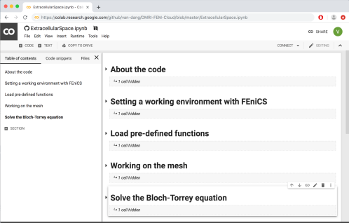
Figure 3: A typical Google Colaboratory notebook for diffusion MRI simulation.

The installation of FEniCS is quite straightforward in the hosted runtime. The command lines are just the same as the installation on Ubuntu.

⬇

!apt-get install software-properties-common

!add-apt-repository ppa:fenics-packages/fenics

!sudo apt-get update

!apt-get install --no-install-recommends fenics

from dolfin import *; from mshr import *

For longer executions, it is more convenient to connect to the local runtime. To this end, one can execute the following command lines to create a local runtime to which the notebook can connect. This command creates a Docker container from the latest stable FEniCS version at the time of writing, given with the fenics_tag variable. Inside this container, we install a Jupyter extension developed by Google Colaboratory’s developers and then run a Jupyter notebook from within the container on port 8888.

⬇

fenics_tag=2019.1.0.r3 # version of FEniCS image

docker run --name notebook-local -w /home/fenics -v $(pwd):/home/fenics/shared -ti -d -p 127.0.0.1:8888:8888 quay.io/fenicsproject/stable:${fenics_tag} "sudo pip install jupyter_http_over_ws; sudo apt-get install -y gmsh; jupyter serverextension enable --py jupyter_http_over_ws; jupyter-notebook --ip=0.0.0.0 --NotebookApp.allow_origin=’https://colab.research.google.com’ --NotebookApp.port_retries=0 --NotebookApp.allow_root=True --NotebookApp.disable_check_xsrf=True --NotebookApp.token=’’ --NotebookApp.password=’’ --port=8888"

Script-based interface

For the script-based interface with parallel executions, the workspace is available at

https://github.com/van-dang/DMRI-FEM-Cloud/blob/master/GCloudDmriSolver.py

Users can pre-process the inputs for one- and multi-compartment domain by respectively using the functions implemented at

https://github.com/van-dang/DMRI-FEM-Cloud/blob/master/PreprocessingOneCompt.py

https://github.com/van-dang/DMRI-FEM-Cloud/blob/master/PreprocessingMultiCompt.py

This workspace can work with Docker image by launching the following command from a Mac or Linux terminal

⬇

docker run -ti -p 127.0.0.1:8000:8000 -v $(pwd):/home/fenics/shared -w /home/fenics/shared quay.io/fenicsproject/stable:current

However, in the HPC context, Singularity is preferable to Docker due to the security, the accessibility, the portability, and the scheduling issues [33]. Fortunately, it is straightforward to build a Singularity image from a Docker image and for our framework, the command lines are as follows

⬇

wget https://raw.githubusercontent.com/van-dang/DMRI-FEM-Cloud/ singularity_images/Singularity_recipe_FEniCS_DMRI

sudo singularity build -w writable_fenics_dmri.simg Singularity_recipe_FEniCS_DMRI

Code structure

Although the interfaces are different between the web-based and the script-based workspaces, they have similar structures with three main classes

• MRI_parameters manages the diffusion pulses such as sequence type, $b-$values, $g-$value and the conversion between them.

• MRI_domain manages the finite element meshes, function spaces, domain sizes, diffusion tensors, permeability, and boundary markers.

• MRI_simulation manages the initial conditions, time-stepping sizes, linear solvers, solutions, and post-processing.

In MRI_domain, the boolean variable IsDomainMultiple is used to switch between the single-compartment and the multi-compartment domains. Both strong and weak imposition of the pseudo-periodic BCs have some advantages and disadvantages. The strong imposition works efficiently with periodic meshes with higher accuracy compared to the weak imposition. In some cases, it is, however, not practical to generate periodic meshes. We allow for both options by the use of a boolean variable IsDomainPeriodic. When it is True, Eq. (9) is solved, otherwise, Eq. (1) is solved.

In what follows, we show how to define an arbitrary diffusion sequence and how to use partition_marker to define some input parameters on heterogeneous domains.

General diffusion-encoding sequence

The framework allows for arbitrary temporal profiles $f(t)$. During the simulation, we need to compute its integral $\displaystyle\mathcal{F}(t)=\int_{0}^{t}f(s)\,ds$ and convert between $b-$value and the gradient strength $g-$value following Eq. (6). In the Python version, SymPy is used to compute the symbolic integration. So, users only need to provide the expression of $f(s)$ to the function member fs_sym of the class MRI_parameters(). $\mathcal{F}(t)$ and the conversion between $b-$value, $g-$value are automatically done. For example, a cos-OGSE sequence

$$f(s)=\begin{cases}\cos(\omega\,s),&\mbox{ if }s\leq\delta\\ -\cos\Bigl{(}\omega(s-\tau)\Bigl{)},&\mbox{ if }\tau<s\leq\delta+\tau\\ 0,&\mbox{otherwise}\end{cases}$$ (7)

with $\displaystyle\omega=\frac{2\,n\pi}{\delta},\tau=\frac{\delta+\Delta}{2}$ can be simply defined as the following

⬇

import sympy as sp

mp = MRI_parameters()

...

mp.delta, mp.Delta = 10000, 10000

mp.T = mp.delta+mp.Delta

mri_para.nperiod = 2

omega = 2.0*mri_para.nperiod*pi/mri_para.delta

tau = mp.T/2.

mri_para.fs_sym = sp.Piecewise(

( sp.cos(omega*mri_para.s) , mri_para.s <= mri_para.delta ),

( 0., mri_para.s <= tau ),

( -sp.cos(omega*(mri_para.s-tau)), mri_para.s <= mri_para.delta + tau ),

( 0., True )

)

...

mp.Apply() # F(t) and the conversion between b and q are done here

Initial conditions

By default, we initialize the spins to be one everywhere. However, it is possible to define discontinuous initial conditions which are illustrated in the following code snippet.

⬇

mri_simu = MRI_simulation()

mri_para = MRI_parameters()

mymesh = Mesh(...)

mri_domain = MRI_domain(mymesh, mri_para)

...

IC_array = [0, 1, 0];

dofmap_DG = mri_domain.V_DG.dofmap()

disc_ic = Function(mri_domain.V_DG);

for cell in cells(mymesh):

cmk = partition_marker[cell.index()]

cell_dof = dofmap_DG.cell_dofs(cell.index())

disc_ic.vector()[cell_dof] = IC_array[cmk];

disc_ic=project(disc_ic, mri_domain.V)

...

mri_simu.solve(mri_domain, mri_para, linsolver, disc_ic)

Diffusion coefficients and tensors

We allow for a general definition of the diffusion tensor with $d\times d$ components

$$\bm{D}(\bm{x})=\Bigl{[}d_{jk}(\bm{x})\Bigl{]}_{j=1..d,k=1..d}$$ (8)

where $d_{jk}(\bm{x})$ is cell-based piecewise continuous. We loop through all elements (cells) and the value can be determined by the coordinates of the cell midpoint p=cell.midpoint() or a given partition_marker.

⬇

partition_marker = MeshFunction("size_t", mesh, mesh.topology().dim())

# define partition markers

...

D0_array=[3e-3, 1e-3, 3e-3]

# Variable diffusion tensor

V_DG=mri_domain.V_DG; dofmap_DG = V_DG.dofmap();

d00 = Function(V_DG); d01 = Function(V_DG); d02 = Function(V_DG)

d10 = Function(V_DG); d11 = Function(V_DG); d12 = Function(V_DG)

d20 = Function(V_DG); d21 = Function(V_DG); d22 = Function(V_DG)

for cell in cells(mymesh):

p = cell.midpoint() # the coordinate of the cell center.

cmk = partition_marker[cell.index()]

cell_dof = dofmap_DG.cell_dofs(cell.index())

d00.vector()[cell_dof] = D0_array[cmk];

d11.vector()[cell_dof] = D0_array[cmk];

d22.vector()[cell_dof] = D0_array[cmk];

mri_domain.ImposeDiffusionTensor(d00,d01,d02,d10,d11,d12,d20,d21,d22)

$T_{2}-$relaxation coefficient

By default $T_{2}-$relaxation is set to be 1e16. However, users can define it similarly to the diffusion entry. The following code shows how to define $T_{2}$ for a three-compartment domain.

⬇

T2_array=[4e16, 4e4, 4e4]

dofmap_DG = mri_domain.V_DG.dofmap()

T2 = Function(mri_domain.V_DG);

for cell in cells(mymesh):

cmk = partition_marker[cell.index()]

cell_dof = dofmap_DG.cell_dofs(cell.index())

T2.vector()[cell_dof] = T2_array[cmk];

mri_para.T2 = T2

3.4 Solution visualization and post-processing

After solving the Bloch-Torrey equation, the solutions are saved, visualized and the signals are computed following Eq. (5) in a routine called PostProcessing. Matplotlib [43] is used for simple visualizations. For more advanced features, Paraview [44] can be externally used for the saved solutions.

4 Numerical validation and comparison

Unless stated otherwise, the simulations were performed for a PGSE with $\Delta=43100\mu\text{s},\delta=10600\mu\text{s}$, $b-$values between 0 and $10000\text{s/mm}^{2}$, and the diffusion coefficient of $D=3\times 10^{-3}\text{mm}^{2}/\text{s}$. The membrane between the compartments, if any, is permeable with the permeability of $\kappa=10^{-5}\text{m}/\text{s}$. The simulated signals are compared to the reference ones computed by the matrix formalism (MF) method [45].

We provide a complete simulation method of diffusion inside the multilayered structures such as concentric disks, cylinders, spheres, and torus with the mesh generation software GMSH [38].

First, we study diffusion inside a three-layered disk of $[5,7.5,10]\mu\text{m}$ with different settings of the initial conditions. Fig. 4a shows the setting IC_array=[0, 1, 0] as discussed in Section 3.3. The solver is available at

https://colab.research.google.com/github/van-dang/DMRI-FEM-Cloud/blob/master/DiscontinuousInitialCondition.ipynb

The time step size of $\Delta t=200\mu\text{s}$ is used. The signals are shown in Fig. 4b where we show that the signals are strongly dependent on how we set up the initial conditions. The accuracy of the simulations is verified by comparing with the reference signal for the uniform distribution of the initial conditions.

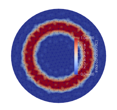
(a) Initial conditions [0, 1, 0]

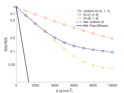
(b) Signals

Figure 4: Simulations of diffusion inside a three-layered disk of $[5,7.5,10]\mu\text{m}$ with different settings of the initial conditions for a PGSE sequence with $\Delta=43100\mu\text{s}$ and $\delta=10600\mu\text{s}$. Fig (a) show the initial conditions with [0, 1, 0]. The signals are strongly dependent on how the initial conditions are set up (b). The accuracy of the simulations is verified by comparing with the reference signal for the uniform distribution of the initial conditions.

To reduce the computational domain, one can assume that the domain is periodically repeated and our framework allows for imposing pseudo-periodic BCs. To illustrate this capacity, we consider a square $\Omega=[-5\mu\text{m},5\mu\text{m}]^{2}$ including some permeable periodic cells with the permeability $\kappa=10^{-5}\text{m}/\text{s}$ (see Fig. 5a). The signals were computed for a PGSE with $\Delta=13000\mu\text{s},\delta=10000\mu\text{s},{\bm{q}}=\frac{[1,1,0]}{\sqrt{2}}$ (see Fig. 5b. The solver is available at

https://colab.research.google.com/github/van-dang/DMRI-FEM-Cloud/blob/master/PeriodicDomains.ipynb

We see that the artificial-permeability method approaches the pseudo-periodic BCs. To achieve the same accuracy, the latter only needs $\Delta t=100\mu\text{s}$ which is ten times as larger as the first. So, it is strongly recommended to use Eq. (9) if the domain is periodic. It is, however, important to recall that the first is useful for non-periodic computational boxes.

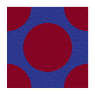
(a) A square box with circular cells

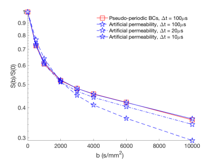
(b) Normalized signals

Figure 5: The artificial permeable method approaches the pseudo-periodic BCs. The time-step size needs to be small to achieve the same accuracy. It is, however, important to recall that the artificial permeable method is useful for non-periodic computational boxes.

We now consider discontinuous diffusion tensors mentioned in Section 3.3 to study diffusion in three-layered structures including a disk, a sphere and a torus whose radii are $5,7.5$ and $10\mu\text{m}$ respectively (see Figs 6a, 6b, and 6c). For the torus, the radius from the center of the hole to the center of the torus tube is $R=20\mu\text{m}$. The simulated signals match very well to the reference signals with the time step size of $\Delta t=200\mu\text{m}$ (see Fig. 6d). The Python source code is available at

https://colab.research.google.com/github/van-dang/DMRI-FEM-Cloud/blob/master/MultilayeredStructures.ipynb

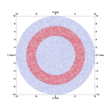
(a) Three-layered disk

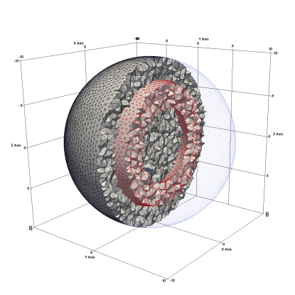
(b) Three-layered sphere

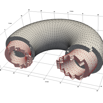
(c) Three-layered torus

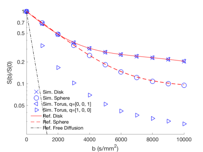
(d) Signals

Figure 6: Three-layered structures and their signals for a PGSE with $\Delta=43100\mu\text{s},\delta=10600\mu\text{s}$. The time step size is $\Delta t=200\mu\text{s}$.

The three-layered cylinder is again used to illustrate the effect of $T_{2}-$relaxation to the magnetization and the signal attenuation. The gradient direction is $\bm{q}=[0,1,0]$ which is perpendicular to the cylinder axis. As expected, the transverse magnetization decays faster for smaller $T_{2}$ (Figs. 7a, 7b, 7c). The signals $S(b)$ are quite different when $T_{2}$ varies (Fig. 7d). Here we also show that our signals approximate accurately the reference ones calculated by the matrix formalism (solid curve in the figure) [45]. In short, $T_{2}-$relaxation can be used as one of the sources of the image contrast.

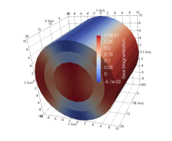
(a) $T_{2}=\text{[}\infty,\infty,\infty\text{]}$

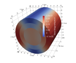
(b) $T_{2}=\text{[}40\,{\rm ms},\infty,\infty\text{]}$

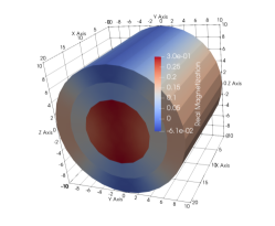
(c) $T_{2}=\text{[}\infty,40,40\text{]\,{\rm ms}}$

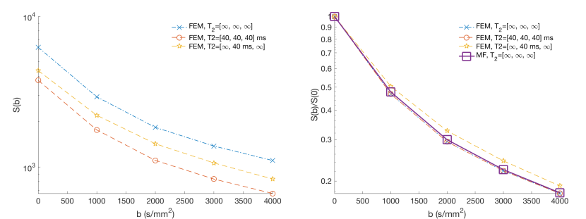
(d) Signals

Figure 7: $T_{2}-$effects of diffusion inside a three-layered cylinder for a PGSE with $\Delta=\delta=10\rm ms$, permeability $\kappa=10^{-5}\text{m}/\text{s}$ to the magnetization at $b=4000\text{s/mm}^{2}$ (a, b, c), and to the signals for $b$ between 0 and $4000\text{s/mm}^{2}$ (d).

The Python source code is available at

https://colab.research.google.com/github/van-dang/DMRI-FEM-Cloud/blob/master/T2_Relaxation.ipynb

Now, we use the solver to compare the signals inside a disk of radius $5\mu\text{m}$ for some temporal profiles: PGSE, Double PGSE, cos-OGSE, sin-OGSE, Trapezoidal PGSE, and Double Trapezoidal PGSE with $\delta=\Delta=10000\mu\text{s}$ (see Fig. 8b). The solver is available at

https://colab.research.google.com/github/van-dang/DMRI-FEM-Cloud/blob/master/ArbitraryTimeSequence.ipynb

The simulated signals match very well the reference signals for the PGSE and cos-OGSE. The signals with OGSE sequences decay faster compared to the others (see Fig. 8a).

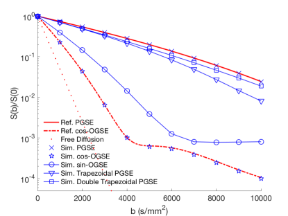
(a) Signals

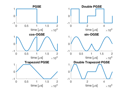
(b) Temporal profiles

Figure 8: Simulated signals inside a disk of radius $5\mu\text{m}$ (a) for different temporal profiles: PGSE, Double PGSE, cos-OGSE, sin-OGSE, Trapezoidal PGSE, and Double Trapezoidal PGSE with $\delta=\Delta=10000\mu\text{s}$ (b). The simulated signals match very well the reference signals for the PGSE and cos-OGSE. The signals with OGSE sequences decay faster compared to the others.

5 Simulation examples

5.1 Realistic neurons

We consider a population of 36 pyramidal and 29 spindle neurons. They are distributed in the anterior frontal insula (aFI) and the anterior cingulate cortex (ACC) of the neocortex of the human brain. They share some morphological similarities such as having a single soma and dendrites branching on opposite sides. This population consists of 20 neurons for each type in aFI, and 9 spindles, 16 pyramidals in ACC. We have published these volume meshes at

https://github.com/van-dang/RealNeuronMeshes

The solver is available at

https://colab.research.google.com/github/van-dang/DMRI-FEM-Cloud/blob/master/RealNeurons.ipynb

Table 1 shows the computational time in minutes of neuron simulations on Google Colaboratory for a PGSE sequence with $\Delta=43100\mu\text{s},\delta=10600\mu\text{s}$, $b=4000\,\text{s/mm}^{2}$ and two different time step sizes $\Delta t=50,100\mu\text{s}$. The relative difference in signals between them is within 4%. With $\Delta=100\mu\text{s}$ it costs about an hour for the largest neuron with 615146 vertices whereas it costs only 3 minutes with a small neuron with 27811 vertices.

Neuron	Mesh size	$\Delta t=50\mu\text{s}$	$\Delta t=100\mu\text{s}$
04b_pyramidal7aACC	615146 vertices	119	64
25o_spindle17aFI	51792 vertices	21	10
03b_pyramidal2aACC	27811 vertices	6	3

Table 1: Timing in minutes of neuron simulations on Google Colaboratory for a PGSE sequence with $\Delta=43100\mu\text{s},\delta=10600\mu\text{s}$ and different time step sizes $\Delta t$.

In addition to the standard approach using volume elements, we also allow for simulating on manifolds following the method developed in [17]. Figure 9 shows a comparison between signals inside a neuron from the drosophila melanogaster for a standard 3D mesh and the corresponding 1D manifolds. For $\Delta t=200\mu\text{s}$, it costs only 3 seconds for 1D manifolds but 380 seconds for 3D to compute the signal for one $b-$values with the same accuracy.

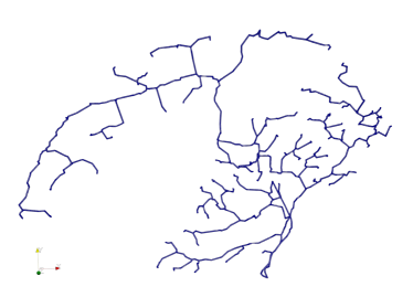
(a)

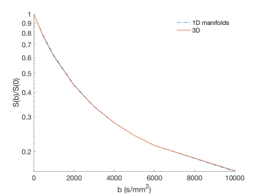
(b)

Figure 9: A comparison between signals inside a neuron from the drosophila melanogaster for a standard 3D mesh and the corresponding 1D manifolds. For $\Delta t=200\mu\text{s}$, it costs only 3 seconds for 1D manifolds but 380 seconds for 3D to compute the signal for one $b-$values with the same accuracy.

For more details, it is recommended to look at the solver available at

https://colab.research.google.com/github/van-dang/DMRI-FEM-Cloud/blob/master/Manifolds.ipynb

5.2 Extracellular space

It is challenging to perform simulations on extracellular space (ECS) due to the geometrical complexity. The thickness of ECS is tiny compared to the computational domain. It is extremely time-consuming to use Monte-Carlo approaches. If the reflection condition is applied, the particle undergoes multiple reflections until no further surface intersections are detected, and if the rejection method is applied, the time step sizes need to be very small to be accurate.

In this section, we show that it is efficient to use our framework. We tested with the ECS extracted from the medical segmentation published at http://synapseweb.clm.utexas.edu/2013kinney (see also [46]). The volume mesh is shown in Fig. 10a with 462420 vertices and 926058 tetrahedrons

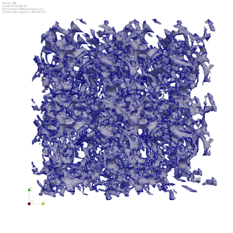
(a)

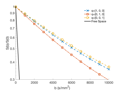
(b)

Figure 10: The mesh of an extracellular space with 462420 vertices and 926058 tetrahedrons (a). It was reconstructed from the medical segmentation published at http://synapseweb.clm.utexas.edu/2013kinney (see also [46]). Two directions in the $xz-$plane give quite similar signals showing that the domain is quite isotropic in these directions and they both are distinguishable to the signals in the $y-$direction (b).

The processed meshes are available in the following link

https://github.com/van-dang/DMRI-FEM-Cloud/raw/mesh/2E_ExtraCellular_group_10um_vol.xml.zip

The Google Colab-based solver is available in the following link

https://colab.research.google.com/github/van-dang/DMRI-FEM-Cloud/blob/master/ExtracellularSpace.ipynb

The timing per $b-$value is about 30 minutes on Google Colaboratory for the time discretization $\Delta t=1\,\rm ms$. With half of this time-step size, i.e., $\Delta t=500\,\mu\text{s}$, it takes about an hour for $b=10000\text{s/mm}^{2}$ on Google Colaboratory and the difference in the signals compared to $\Delta t=1000\,\mu\text{s}$ is only 1%. The signals for three principle gradient directions are shown in Fig. 10b. Two directions in the $xz-$plane give quite similar signals showing that the domain is quite isotropic in these directions and they both are distinguishable from the signals in the $y-$direction.

5.3 Parallelization

Now we verify the simulation performance with the Singularity image on a 12-month free trial of Google Cloud Platform (https://cloud.google.com) and Tegner (PDC - KTH). The script-based interface is used. It shares the core functionalities with the Python Notebook interface and supports all the functionalities discussed in the paper except the artificial permeability implementation which is still in development. So, the mesh needs to be periodic to have the pseudo-periodic BCs in the parallel execution.

First, we show the simulation performance on one computational node on the neuron 04b_pyramidal7aACC (Fig. 11a) with the mesh size of about 0.6M vertices (2.5M tetrahedrons) and the time discretization of $\Delta t=200\mu\text{s}$. A PGSE with $\Delta=43100\mu\text{s},\delta=10600\mu\text{s}$ is used. The commands to execute the simulation with the FEniCS image are follows

⬇

singularity exec -B $PWD writable_fenics_dmri.simg python3 PreprocessingOneCompt.py -o onecompt_files.h5

ListNumProcs="2 4 6 8" # one-node in Google Cloud

ListNumProcs="5 10 15 20" # one-node in Tegner

for p in ${ListNumProcs}

do

singularity exec -B $PWD writable_fenics_dmri.simg mpirun -n ${p} python3 GCloudDmriSolver.py -f onecompt_files.h5 -M 0 -b 1000 -d 10600 -D 43100 -k 200 -K 3e-3 -gdir 1 0 0

done

On Tegner with 20 processors, it costs about 7 minutes per one $b-$value whereas on Google Cloud with 8 processors, it costs about 30 minutes.

Then, we verify with 25 computational nodes on the sample presented in Section 7.6 [16]. The sample consists of a pyramidal neuron of an adult female mouse [47] embedded in the center of a computational domain $\Omega=[-300,300]\times[-250,250]\times[-100,100]\,\mu\text{m}^{3}$ (Fig. 11b). We assume that there is a permeable membrane with $\kappa=10^{-5}\text{m}/\text{s}$ between the neuron and the extracellular space. The whole mesh (box + neuron) has about 1.5M vertices (8.5M tetrahedrons). The neuron itself consists of 131996 vertices and 431326 tetrahedrons. The whole mesh and sub-mesh (neuron) are available for download at

https://github.com/van-dang/DMRI-FEM-Cloud/raw/mesh/volume_box_N_18_7_3_5L_fine.xml.zip https://github.com/van-dang/DMRI-FEM-Cloud/raw/mesh/volume_N_18_7_3_5L_fine.xml.zip

Below are the commands to execute the simulation with the FEniCS image

⬇

singularity exec -B $PWD writable_fenics_dmri.simg python3 PreprocessingMultiCompt.py -o multcompt_files.h5

ListNumProcs="100 210 300 500" # 25 nodes in Tegner

for p in ${ListNumProcs}

do

mpirun -n $p singularity exec -B $PWD writable_fenics_dmri.simg python3 GCloudDmriSolver.py -f multcompt_files.h5 -M 1 -b 1000 -p 1e-5 -d 10600 -D 43100 -k 200 -gdir 0 1 0

The simulation with 500 processors costs about 20 minutes per $b-$value with $\Delta t=200\mu\text{s}$.

The strong parallel scaling is shown in Fig. 11c. Here $T_{p}$ indicates the timing for $p$ processors, $p_{0}=5$ for the first case and $p_{0}=100$ for the latter. The scaling for FEniCS on Tegner is good both on one-node (32 CPUs) and multi-node (scaling up to 500 CPUs). For a small number of cores (2,4,6,8) on Google Cloud, for this specific case with a fine mesh size of 2.5M tetrahedrons, the work and data partition per process are greatly exceeding the ideal work and data per process ratio. The scaling is less good in comparison with the ideal linear scaling.

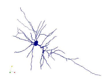
(a) Neuron 04b_pyramidal7aACC

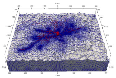
(b) The mouse neuron embedded in a box

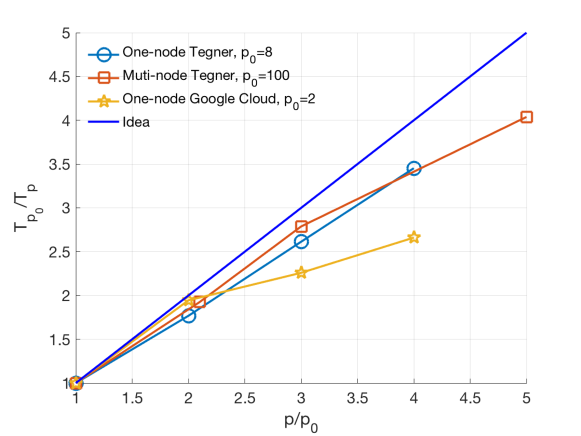
(c) Strong parallel scaling of one-node and multi-node simulations

Figure 11: The simulation performance is verified for a single computational node on the neuron 04b_pyramidal7aACC and for multiples nodes on the mouse neuron embedded in a box presented in Section 7.6 in [16]. The strong scaling on Tegner is good both on one node (32 CPUs) and multi-node (scaling up to 500 CPUs). For a small number of cores (2, 4, 6, 8) on Google Cloud, for this specific case with a fine mesh size of 2.5M tetrahedrons, the work and data partition per process are greatly exceeding the ideal work and data per process ratio. The scaling is less good in comparison with the ideal linear scaling.

6 Discussion

The proposed framework can be viewed as the Python version of the Matlab-based SpinDoctor. In this paper, we focused on advanced software features such as portability and parallelization. This framework inherits all of the PDE solution functionalities of FEniCS, thus, extensions and generalizations of the present dMRI simulation problem, including the coupling with flow, the simulation on deforming domains like the heart, or the coupling of simulations in manifolds with simulations in 3D domains, are rather straightforward.

Similar to SpinDoctor, the present framework is supposed to be faster and more accurate than Monte-Carlo simulation packages such as Camino. More importantly, our approach benefits from a long history of theoretical and numerical developments by the mathematical and engineering communities. It enhances software reliability which is one of the core concerns in medical applications.

As other cloud-based software developments, this framework brings reproducible science and open-source software to computational diffusion MRI. It speeds up the method development process since the results are easy to confirm and new methods can be easily developed on top of the existing methods. New algorithms written as Google Colaboratory notebooks can quickly circulate in the MRI community and this allows for active collaboration between research groups.

Since SpinDoctor couples the finite elements discretization with optimized adaptive ODE solvers, it is more efficient than our framework in terms of time discretization. The analogous ODE solvers written in Python can be found in the SciPy Library [48] but they are not ready to use within our framework: they do not yet efficiently support the mass matrix and the sparse Jacobian matrix. The lumped mass matrix approach can be used to fix the first issue but more investigations are needed to resolve the latter issue.

Generating finite elements meshes from medical segmentation is very challenging. Complicated surface meshes currently need to be processed outside the framework to obtain a good quality finite elements mesh. Streamlining this process is an interesting direction of future investigation and it may be well worthwhile to develop algorithms to automate this process.

7 Conclusions

We proposed a portable simulation framework for computational diffusion MRI that works efficiently with cloud technology. The framework can be seamlessly integrated with cloud computing resources such as Google Colaboratory notebooks working on a web browser or with Google Cloud Platform with MPI parallelization. Many simulation needs of the field were addressed by the use of advanced finite element methods for both single- and muti-compartment diffusion domains, with or without permeable membrane and periodic boundaries. We showed the accuracy, the computational times, and parallel computing capabilities through a set of examples, while mentioning straightforward future extensions. The framework contributes to reproducible science and open-source software in computational diffusion MRI. We hope that it will help to speed up method developments and stimulate research collaborations.

Appendices

The methods imposed in our framework are based on the partition of unity finite element method (PUFEM) to manage the interface conditions [16]. Both weak and strong implementation of the periodicity with some advantages and disadvantages are included. The $\theta-$method is used for the time discretization.

Appendix A Strong implementation of the pseudo-periodic BCs

The complex-valued and time-dependent term in the pseudo-periodic boundaries make it too difficult to implement in a standard FEM software package. So, one can transform the pseudo-periodic BCs to the periodic ones. Following [10, 12], one can choose to transform the magnetization to a new unknown $u(\bm{x},t)$:

$$u(\bm{x},t)=U(\bm{x},t)\,e^{i\,\,\gamma\,\mathcal{F}(t)\,\bm{g}\cdot\bm{x}}$$

The Bloch-Torrey PDE (1) is then transformed to [12]

$$\frac{\partial u}{\partial t}=-i\,\gamma\,\mathcal{F}\Bigl{(}\bm{g}\cdot{\bm{D}}\nabla u+\nabla u\cdot{\bm{D}}\,\bm{g}\Bigl{)}-\Bigl{(}\gamma\,\mathcal{F}\Bigl{)}^{2}{\bm{g}}\cdot\bm{D}\,{\bm{g}}\,u-\frac{u}{T_{2}}+\nabla\cdot\Bigl{(}\bm{D}\nabla u\Bigl{)},$$ (9)

with periodic BCs

$$u_{m} =u_{s}$$ (10)

$${\bm{D}}_{m}\nabla u_{m}\cdot\bm{n} ={\bm{D}}_{s}\nabla u_{s}\cdot\bm{n}$$

The homogeneous Neumann boundary condition of $U$ leads to

$$\bm{D}\nabla u\cdot\bm{n}=i\,\gamma\,\mathcal{F}\,u\,\bm{D}\,\bm{g}\cdot\bm{n}.$$

The interface conditions (Eq. 2) are changed to

$$\Bigl{\llbracket}\bm{D}\nabla u\cdot\bm{n}_{0}\Bigl{\rrbracket} =2\,i\,\gamma\,\mathcal{F}\Bigl{\{}u\,\bm{D}\,\bm{g}\cdot\bm{n}_{0}\Bigl{\}}.$$ (11)

$$\Bigl{\{}\bm{D}\nabla u\cdot\bm{n}_{0}\Bigl{\}} =-\kappa\llbracket u\rrbracket+\frac{i\,\gamma\,\mathcal{F}}{2}\llbracket u\,\bm{D}\,\bm{g}\cdot\bm{n}_{0}\rrbracket.$$

Since the magnetization is discontinuous ($m_{0}\neq m_{1}$ on the interface), Eq. (11) shows the flux is also discontinuous.

Following the same PUFEM approach proposed in [16], we obtain the following weak form

$$\Biggl{(}\frac{\partial}{\partial t}u,v\Biggl{)}_{\Omega_{0}\cup\Omega_{1}}=F(u,v,t).$$

where

$$F(u,v,t)=-\Biggl{(}i\,\gamma\,\mathcal{F}\,\Bigl{(}{\bm{g}}\cdot\bm{D}\,\nabla u+\nabla u\cdot\bm{D}\,{\bm{g}}\Bigl{)},v\Biggl{)}_{\Omega_{0}\cup\Omega_{1}}\\ -\Biggl{(}\bigl{(}\gamma\,\mathcal{F}\bigl{)}^{2}\,{\bm{g}}\cdot\bm{D}\,{\bm{g}}\,u+\frac{u}{T_{2}},v\Biggl{)}_{\Omega_{0}\cup\Omega_{1}}-\Biggl{(}\bm{D}\nabla u,\nabla v\Biggl{)}_{\Omega_{0}\cup\Omega_{1}}\\ +\Biggl{<}-\kappa\llbracket u\rrbracket+\frac{i\,\gamma\,\mathcal{F}}{2}\Bigl{\llbracket}u\,\bm{D}\,\bm{g}\cdot\bm{n}_{0}\Bigl{\rrbracket},\llbracket v\rrbracket\Biggl{>}_{\Gamma}+\Biggl{<}2\,i\,\gamma\,\mathcal{F}\Bigl{\{}u\,\bm{D}\,\bm{g}\cdot\bm{n}_{0}\Bigl{\}},\{v\}\Biggl{>}_{\Gamma}\\ +\Biggl{<}i\,\gamma\,\mathcal{F}\,u\,\bm{D}\,\bm{g}\cdot\bm{n},v\Biggl{>}_{\Gamma^{N}_{0}\cup\Gamma^{N}_{1}}.$$ (12)

We consider a partition of the time domain $0=t_{0}<t_{1}<\dots<t_{N}=T$ associated with the time intervals $I_{n}=(t^{n-1},t^{n}]$ of length $k^{n}=t^{n}-t^{n-1}$ and $u^{n}$ be an approximation of $u(\bm{x},t)$ for a given a triangulation $\mathcal{T}^{h}$ at $t=t^{n}$.

The PUFEM with the time-stepping $\theta-$method is stated as: Find $u^{n}_{h}=(u^{n}_{h,0},u^{n}_{h,1})\in\bm{V}_{h}$ such that

$$\Biggl{(}\frac{u^{n}_{h}-u^{n-1}_{h}}{k^{n}},v_{h}\Biggl{)}_{\Omega_{0}\cup\Omega_{1}}=\theta\,F(u^{n}_{h},v_{h},t^{n})+(1-\theta)\,F(u^{n-1}_{h},v_{h},t^{n-1})$$ (13)

for all $v_{h}=(v_{0,h},v_{1,h})\in\bm{V}_{h}$, where

$$\Bigl{(}a,b\Bigl{)}_{\Omega_{0,h}\cup\Omega_{1,h}}=\Bigl{(}(1-\Phi_{h})\,a_{0},b_{0}\Bigl{)}_{\Omega_{h}}+\Bigl{(}\Phi_{h}a_{1},b_{1}\Bigl{)}_{\Omega_{h}},$$

and $\Phi_{h}$ is an element-wise constant function:

$$\Phi_{h}=\begin{cases}1&\mbox{ in }\Omega_{1,h}\\ 0&\mbox{ in }\Omega_{0,h}\end{cases}$$ (14)

The bilinear and linear forms are defined by

$$\bm{a}(u^{n}_{h},v_{h}) =\Biggl{(}\frac{u^{n}_{h}}{k^{n}},v_{h}\Biggl{)}_{\Omega_{0}\cup\Omega_{1}}-\theta\,F(u^{n}_{h},v_{h},t^{n})$$ (15)

$$\bm{L}(v_{h}) =\Biggl{(}\frac{u^{n-1}_{h}}{k^{n}},v_{h}\Biggl{)}_{\Omega_{0,h}\cup\Omega_{1,h}}+(1-\theta)\,F\biggl{(}u^{n-1}_{h},v_{h},t^{n-1}\biggl{)}$$

Appendix B Weak implementation of the pseudo-periodic BCs

The pseudo-periodic BCs (Eq. 4) can be implemented weakly through the use of an artificial permeability coefficient, $\kappa^{e}$ [15, 16]. The artificial permeability condition at the external boundaries take two equations for the master side and the slave side of the mesh. For the master side, it has the following form

$$\bm{D}_{m}\nabla U_{m}\cdot\bm{n}_{m}=\kappa^{e}\Bigl{(}U_{s}\,e^{i\,\theta_{ms}}-U_{m}\Bigl{)},$$ (16)

and for the slave-side it has the following form

$$\bm{D}_{s}\nabla u_{s}\cdot\bm{n}_{s}=\kappa^{e}\Bigl{(}U_{m}\,e^{i\,\theta_{sm}}-U_{s}\Bigl{)},$$ (17)

where $U_{s}=U(\bm{x}_{s}),U_{m}=U(\bm{x}_{m})$, $\theta_{ms}=-\theta_{sm}=\gamma\;\bm{g}\cdot(\bm{x}_{s}-\bm{x}_{m})\,\mathcal{F}(t)$. When the master side is considered (Eq. 16), $\bm{x}_{m}$ is the mesh point and $\bm{x}_{s}$ is the projection of $\bm{x}_{m}$ onto the slave side. Similarly, when the slave side is considered (Eq. 17), $\bm{x}_{s}$ is the mesh point and $\bm{x}_{m}$ is the projection of $\bm{x}_{s}$ onto the master side. So, the points always align each other but they do not need to be the mesh grid at the same time. So, this method allows for non-matching meshes.

The artificial permeability coefficient $\kappa^{e}$ can be chosen to be consistent with the Nitsche’s method for the Dirichlet BCs [49] (see also a review in [50] and references therein), i.e $\kappa^{e}=\max\Bigl{\{}\frac{\bm{D}}{h}\Bigl{\}}$ where $h$ is the element size.

To overcome the CFL constraints, the following operator splitting can be used to have an unconditionally stable scheme

$$\bm{D}_{m}\nabla U_{m}\cdot\bm{n}_{m}\approx\kappa^{e}\Bigl{(}U_{s}^{n-1}\,e^{i\,\theta_{ms}^{n}}-U_{m}^{n}\Bigl{)},$$ (18)

$$\bm{D}_{s}\nabla U_{s}\cdot\bm{n}_{s}\approx\kappa^{e}\Bigl{(}U_{m}^{n-1}\,e^{i\,\theta_{sm}^{n}}-U_{s}^{n}\Bigl{)}.$$

where $U^{n}$ and $U^{n-1}$ are the approximations at the current and previous time step respectively.

Without imposing the weak pseudo-periodic, the PUFEM with the time-stepping $\theta-$method is stated as: Find $U^{n}=(U^{n}_{0},U^{n}_{1})\in\bm{V}^{h}$ such that

$$\Biggl{(}\frac{U^{n}-U^{n-1}}{k^{n}},v^{h}\Biggl{)}_{\Omega_{0}\cup\Omega_{1}}=\theta\,F(U^{n},v^{h},t^{n})+(1-\theta)\,F(U^{n-1},v^{h},t^{n-1})$$ (19)

for all $v^{h}=(v^{h}_{0},v^{h}_{1})\in\bm{V}^{h}$, where

$$F(U,v,t)=\Biggl{(}-i\,\gamma f(t)\,\bm{g}\cdot\bm{x}\,U-\frac{U}{T_{2}},v\Biggl{)}_{\Omega_{0}\cup\Omega_{1}}-\Bigl{(}\bm{D}\,\nabla U,\nabla v\Bigl{)}_{\Omega_{0}\cup\Omega_{1}}-\kappa\Bigl{<}\llbracket U\bigl{\rrbracket},\llbracket v\bigl{\rrbracket}\Bigl{>},$$ (20)

and $\Bigl{(}a,b\Bigl{)}_{\Omega_{0}^{h}\cup\Omega_{1}^{h}}=\Bigl{(}(1-\Phi^{h})\,a_{0},b_{0}\Bigl{)}_{\Omega^{h}}+\Bigl{(}\Phi^{h}a_{1},b_{1}\Bigl{)}_{\Omega^{h}}$, $\Phi^{h}$ is an element-wise constant function.

The bilinear and linear forms are defined by

$$\bm{a}(U^{n},v^{h}) =\Biggl{(}\frac{U^{n}}{k^{n}},v^{h}\Biggl{)}_{\Omega_{0}\cup\Omega_{1}}-\theta\,F(U^{n},v^{h},t^{n})$$ (21)

$$\bm{L}(v^{h}) =\Biggl{(}\frac{U^{n-1}}{k^{n}},v^{h}\Biggl{)}_{\Omega_{0}\cup\Omega_{1}}+(1-\theta)\,F\biggl{(}U^{n-1},v^{h},t^{n-1}\biggl{)}$$

The linear system of equations corresponding to the bilinear and linear forms (Eq. 21) is

$$\bm{A}\,{\bm{U}^{n}}=\bm{F}$$ (22)

where

$$\bm{A}=\bm{M}\,{(k^{n})^{-1}}-\theta\Biggl{(}-\Bigl{(}i\,\gamma\,f^{n}+\frac{1}{T_{2}}\Bigl{)}\,\bm{J}-\bm{S}-\bm{I}\Biggl{)}$$ (23)

Here $\bm{M}$ and $\bm{S}$ are referred to as the mass and stiffness matrices respectively, $\bm{J}$ and $\bm{I}$ are corresponding to the first and third terms on the right-hand side of $F$ (Eq. 20), i.e $(\bm{g}\cdot\bm{x}\,U,v)$ and $\kappa\Bigl{<}\llbracket U\bigl{\rrbracket},\llbracket v\bigl{\rrbracket}\Bigl{>}$.

To impose the weak periodic BCs, we plug Eq. (18) to the linear and bilinear forms

$$\bm{a}^{*}(U^{n}_{h},v_{h})=a(U^{n}_{h},v_{h})+\theta\kappa^{e}\Biggl{(}\Bigl{<}U^{n}_{h},v_{h}\Bigl{>}_{\Gamma_{m}^{0}\cup\Gamma_{m}^{1}}+\Bigl{<}U^{n}_{h},v_{h}\Bigl{>}_{\Gamma_{s}^{0}\cup\Gamma_{s}^{1}}\Biggl{)}$$

$$\bm{L}^{*}(v_{h})=L(v_{h})+(1-\theta)\kappa^{e}\Biggl{(}\Bigl{<}U^{n-1}_{s,h}\,e^{i\,\theta_{ms}^{n}},v_{h}\Bigl{>}_{\Gamma_{m}^{0}\cup\Gamma_{m}^{1}}+\Bigl{<}U^{n-1}_{m,h}\,e^{i\,\theta_{sm}^{n}},v_{h}\Bigl{>}_{\Gamma_{s}^{0}\cup\Gamma_{s}^{1}}\Biggl{)}$$