fgivenx: A Python package for functional posterior plotting

Summary

Researchers are often concerned with numerical values of parameters in numerical models. Our knowledge of such things can be quantified and presented using probability distributions as demonstrated in Figure 1.

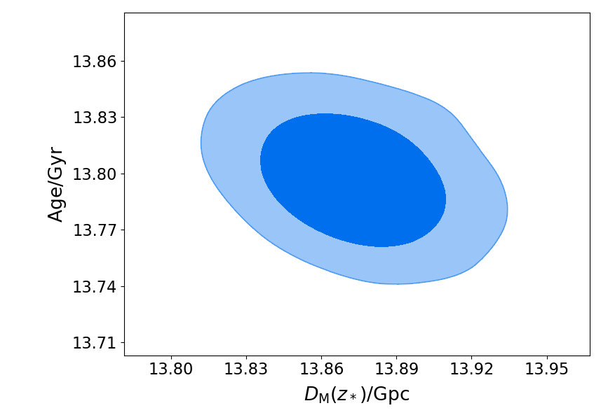
Figure 1: The age and size of the universe, as measured using Planck 2018 data. (non-Astro)Physicists may note that 14 Gigaparsecs is roughly 46 billion light years. The fact that the observable universe is roughly three times larger in light years in comparison with its age is explained by the expansion of space over cosmic history. Contours indicate 67% and 95% marginalised iso-probability credibility regions.

Contour plots such as Figure 1 can be created using two-dimensional kernel density estimation using packages such as https://docs.scipy.org/doc/scipy/reference/generated/scipy.stats.gaussian_kde.htmlhttps://doi.orgscipy (Jones, Oliphant, and Peterson 2001), http://getdist.readthedocs.io/en/latest/intro.htmlhttps://doi.orggetdist (Lewis 2015), https://corner.readthedocs.io/en/latest/https://doi.orgcorner (Foreman-Mackey 2016) and https://pygtc.readthedocs.io/en/latest/https://doi.orgpygtc (Bocquet and Carter 2016), where the samples provided as inputs to such programs are typically created by a Markov Chain Monte Carlo (MCMC) analysis. For further information on MCMC and Bayesian analysis in general, “Information Theory, Inference and Learning Algorithms” is highly recommended (MacKay 2002), which is available freely http://www.inference.org.uk/itprnn/book.htmlhttps://doi.orgonline.

As well as quantifying the uncertainty of real-valued parameters, scientists may also be interested in producing a probability distribution for the predictive posterior of a function f(x). Take as a universally-relatable case the equation of a line y = m*x + c. Given posterior probability distributions for the gradient m and intercept c, then the ability to predict y knowing x given their linear relationship would also be characterized by some uncertainty. This is depicted as P(y|x) in the bottom right panel of Figure 2.

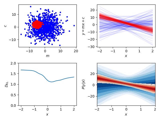
Figure 2: Example output of fgivenx provided some prior and posterior samples and a linear test function. Top-left: underlying parameter covariances between m and c for realizations from the prior (blue) and from the posterior (red). Top-right realisations function y=m*x+c. Bottom-left: The conditional Kullback-Leibler divergence. Bottom-right: The probability of measuring y for a given x, essential a contour version of the panel directly above, where contours indicate 67%, 95% and 99% iso-probability credibility regions.

fgivenx is a Python package for showing the relationships as depicted in Figure 2, including the conditional Kullback-Leibler divergence (Kullback and Leibler 1951). This y=m*x+c example provides a simple illustration, but the code has been used in recent Planck studies to quantify our knowledge of the primordial power spectrum of curvature perturbations (Planck Collaboration 2016)(Planck Collaboration 2018a)(Planck Collaboration 2018b), in examining the dark energy equation of state (Hee et al. 2016) (Hee et al. 2017) for measuring errors in parameter estimation (Higson et al. 2017), for providing diagnostic tests for nested sampling (Higson et al. 2018b) and for Bayesian compressive sensing (Higson et al. 2018a).

fgivenx is a Python package for functional posterior plotting, currently used in astronomy, but will be of use to scientists performing any Bayesian analysis which has predictive posteriors that are functions. The source code for fgivenx is available on https://github.com/williamjameshandley/fgivenxhttps://doi.orgGitHub and has been archived as v2.1.17 to Zenodo with the linked DOI: (Handley 2018).

References

Bocquet, Sebastian, and Faustin W. Carter. 2016. “Pygtc: Beautiful Parameter Covariance Plots (Aka. Giant Triangle Confusograms).” The Journal of Open Source Software 1 (6). https://doi.org/10.21105/joss.00046.

Foreman-Mackey, Daniel. 2016. “Corner.py: Scatterplot Matrices in Python.” The Journal of Open Source Software 24. https://doi.org/10.21105/joss.00024.

Handley, W. 2018. “Fgivenx: V2.1.17,” August. https://doi.org/10.5281/zenodo.1404584.

Hee, S., W. J. Handley, M. P. Hobson, and A. N. Lasenby. 2016. “Bayesian model selection without evidences: application to the dark energy equation-of-state.” MNRAS 455 (January): 2461–73. https://doi.org/10.1093/mnras/stv2217.

Hee, S., J. A. Vázquez, W. J. Handley, M. P. Hobson, and A. N. Lasenby. 2017. “Constraining the dark energy equation of state using Bayes theorem and the Kullback-Leibler divergence.” MNRAS 466 (April): 369–77. https://doi.org/10.1093/mnras/stw3102.

Higson, E., W. Handley, M. Hobson, and A. Lasenby. 2018a. “Bayesian Sparse Reconstruction: A Brute-Force Approach to Astronomical Imaging and Machine Learning.”

———. 2017. “Sampling Errors in Nested Sampling Parameter Estimation.” ArXiv E-Prints, March. http://arxiv.org/abs/1703.09701.

———. 2018b. “Diagnostic Tests for Nested Sampling Calculations.” ArXiv E-Prints, April. http://arxiv.org/abs/1804.06406.

Jones, Eric, Travis Oliphant, and Pearu Peterson. 2001. “SciPy: Open Source Scientific Tools for Python.” http://www.scipy.org/.

Kullback, S., and R. A. Leibler. 1951. “On Information and Sufficiency.” Ann. Math. Statist. 22 (1): 79–86. https://doi.org/10.1214/aoms/1177729694.

Lewis, Anthony. 2015. “Getdist Github Repository.” https://github.com/cmbant/getdist.

MacKay, David J. C. 2002. Information Theory, Inference & Learning Algorithms. New York, NY, USA: Cambridge University Press.

Planck Collaboration. 2016. “Planck 2015 results. XX. Constraints on inflation.” A&A 594 (September): A20. https://doi.org/10.1051/0004-6361/201525898.

———. 2018a. “Planck 2018 results. I. Overview and the cosmological legacy of Planck.” ArXiv E-Prints, July. http://arxiv.org/abs/1807.06205.

———. 2018b. “Planck 2018 results. X. Constraints on inflation.” ArXiv E-Prints, July. http://arxiv.org/abs/1807.06211.