The dynamic critical exponent $z$ of the three-dimensional Ising universality class: Monte Carlo simulations of the improved Blume-Capel model

Abstract

We study purely dissipative relaxational dynamics in the three-dimensional Ising universality class. To this end, we simulate the improved Blume-Capel model on the simple cubic lattice by using local algorithms. We perform a finite size scaling analysis of the integrated autocorrelation time of the magnetic susceptibility in equilibrium at the critical point. We obtain $z=2.0245(15)$ for the dynamic critical exponent. As a complement, fully magnetized configurations are suddenly quenched to the critical temperature, giving consistent results for the dynamic critical exponent. Furthermore, our estimate of $z$ is fully consistent with recent field theoretic results.

I Introduction

In the neighborhood of a second order phase transition, thermodynamic quantities diverge, following power laws. For example, the correlation length $\xi$ diverges as

$$\xi=f_{\pm}|t|^{-\nu}\;\left(1+a_{\pm}|t|^{\theta}+bt+...\right)\;,$$ (1)

where $t=(T-T_{c})/T_{c}$ is the reduced temperature and $\nu$ the critical exponent of the correlation length. The subscript $\pm$ of the amplitudes $f_{\pm}$ and $a_{\pm}$ indicates the high ($+$) and the low ($-$) temperature phase, respectively. Second order phase transitions are grouped into universality classes. For all transitions within such a class, critical exponents like $\nu$ assume the identical value. These power laws are affected by corrections. There are non-analytic or confluent and analytic ones. Also correction exponents such as $\theta=\omega\nu$ are universal. Amplitudes such as $f_{\pm}$, $a_{\pm}$ and $b$ depend on the microscopic details of the system. However certain combinations, so called amplitude ratios, assume universal values. Universality classes are characterized by the symmetry properties of the order parameter at criticality, the range of the interaction and the spacial dimension of the system. Currently the most accurate estimates of static critical exponents for the universality class of the three-dimensional Ising model are $\nu=0.6299709(40)$, $\eta=0.0362978(20)$, and the exponent of the leading correction $\omega=0.82968(23)$, obtained by the conformal bootstrap method, see ref. Simmons-Duffin:2016wlq and references therein. For reviews on critical phenomena see for example WiKo ; Fisher74 ; Fisher98 ; PeVi .

The concepts of critical phenomena can be extended to dynamic processes. For a seminal review see HoHa77 . In addition to the fundamental characteristics of the static universality class, a dynamic universality class is characterized by the type of the dynamics and whether the energy or the order parameter are conserved. For a detailed discussion of the classification scheme see refs. HoHa77 ; FoMo06 . For a review and a book on the related subject of ageing see CaGa05 ; Malte09 . Here we study purely dissipative relaxational dynamics without conservation of the order parameter or the energy, which is denoted as model A in ref. HoHa77 .

In a numerical study, the dynamics of a lattice model can be studied in various settings. We might consider autocorrelation times $\tau$ of systems in equilibrium or various off equilibrium situations. For example the system can be prepared in a low or high temperature state and then it is, for example, subject to a sudden quench to the critical temperature. In the case of damage spreading, the system is prepared in a spatially inhomogeneous state. The system might also be subject to a slowly varying external field. Here, we consider equilibrium dynamics at the critical point and a sudden quench from a fully magnetized configuration, corresponding to zero temperature, to the critical one.

Roughly speaking, the autocorrelation time $\tau$ is the time needed to generate a statistically independent configuration in a stochastic process at equilibrium. More precise definitions will be given below in section IV. In the neighborhood of a critical point the autocorrelation time increases with increasing correlation length $\xi$. This phenomenon is called critical slowing down. The increase is governed by a power law

$$\tau\simeq\xi^{z}\;,$$ (2)

where $z$ is the dynamic critical exponent. It can not be related to the static exponents. Similar to eq. (1), the power law is subject to corrections. Below we simulate directly at the critical point, where the linear lattice size $L$ takes over the role of the characteristic length scale: $\tau\simeq L^{z}$. The exponent $z$ also governs non-equilibrium dynamics. For a detailed discussion see for example refs. Su76 ; JaScSc89 ; Zheng98 .

Field theoretic results for $z$ relevant to the problem studied here are discussed in section 9 of ref. FoMo06 . However one should notice the considerable progress that has been achieved recently in refs. Me15 ; FRG ; Ad17 .

In ref. HaHoMa72 the dynamic critical exponent $z$ was computed to two-loop order in the $\epsilon$-expansion. The authors express their result as

$$z=2+c\eta\;,$$ (3)

where $c=6\ln(4/3)-1=0.72609\;...$ and $\eta$ is the static critical exponent that governs the decay of the two-point function at criticality. In ref. AnVa84 this result was extended to three-loop order, resulting in $c=0.72609\;(1-0.1885\;\epsilon+...)$, where $d=4-\epsilon$ is the dimension of the system. Based on the fact that the coefficient of $\epsilon$ is small, one might hope that most of the difficulties in analyzing the series are shuffled into $\eta$ and the series of $c$ is, in a vague sense, well behaved.

Recently, the $\epsilon$-expansion has been extended to four-loop Ad17 . Based on this result, in appendix C we obtain $z=2.0243$ for three dimensions, taking also into account the accurate estimates $z=2.1665(12)$ NiBl96 and $z=2.1667(5)$ NiBl00 for two dimensions and $z=2+\epsilon^{\prime}-\frac{1}{2}\epsilon^{\prime 2}+...$, where $d=1+\epsilon^{\prime}$, given in ref. Bausch81 .

In addition to the $\epsilon$-expansion, the problem has been attacked by a perturbative expansion in fixed dimension. The four-loop result for three dimensions Prud97 had been analyzed by the authors by using a Padé resummation, resulting in $z=2.017$, which is consistent with the resummation of the three-loop result Prud92 . However, given the fact that a similar analysis for two dimensions gives $z=2.093$ Prud97 , one might suspect that also the result for three dimensions is too small. This is further corroborated by our analysis given in appendix C. For the application of different resummation schemes to the series see also Prud06 .

Finally let us mention the estimates obtained by using functional renormalization group methods Me15 ; FRG . In ref. Me15 , towards the end of section VI, the authors give their estimate $z\approx 2.025$ for the case of the three-dimensional Ising universality class. In ref. FRG numerical results are presented in table I of the paper. Using three different frequency regulators, the authors get $z=2.024$, $2.024$, and $2.023$, respectively. Without such a regulator $z=2.032$ is obtained. The corresponding results for two dimensions are given in table II of ref. FRG . These are $z=2.16$, $2.15$, and $2.14$ for the three different frequency regulators. Without such a regulator $z=2.28$ is obtained, which is quite far off from the results of refs. NiBl96 ; NiBl00 . This suggests that also in three dimensions, the estimates obtained with a frequency regulators should be more reliable than that without.

In summary, refs. Me15 ; FRG and the analysis of the four-loop $\epsilon$-expansion Ad17 now suggest

$$z\approx 2.024\;,$$ (4)

which is somewhat larger than $z=2.021$ for the three-loop $\epsilon$-expansion and $z=2.017$ for the four-loop expansion in three dimensions fixed, which are cited in table 4 of ref. FoMo06 .

Now let us turn to Monte Carlo (MC) simulations of lattice models. In table 1 we summarize results for the exponent $z$. In most of the papers, the Ising model on the simple cubic lattice has been studied WaLa87 ; WaLa91 ; Muenkel93 ; Ito93 ; Grassberger ; Jaster99 ; Ito00 . In ref. Murase , the Ising model on the body centered cubic (bcc) and face centered cubic (fcc) lattice has been simulated. Finally in ref. Collura , similar to the present work, the improved Blume-Capel model on the simple cubic lattice is studied. Improved means that the parameter of the Blume-Capel model is chosen such that leading corrections to scaling vanish. For the definition of the Blume-Capel model see section II below. In refs. WaLa87 ; WaLa91 equilibrium autocorrelation times are determined. In ref. Grassberger damage spreading is considered. Else short time dynamics is studied. Mostly the simulations are started with an ordered configuration, corresponding to $T=0$, and a sudden quench to $T_{c}$ is performed.

Table 1: We summarize results for the dynamic critical exponent $z$ obtained by Monte Carlo simulations of lattice models. Note that in refs. Ito93 ; Ito00 ; Murase the exponent $\lambda=\beta/\nu z$ is computed that we have converted here by using $\beta/\nu=\Delta_{\sigma}=0.5181489(10)$ in three dimensions Simmons-Duffin:2016wlq . In most of the cases, the Ising model on the simple cubic lattice is simulated. In the case of ref. Murase , the Ising model on the body centered cubic (bcc) and face centered cubic (fcc) lattice is studied. The author of ref. Collura simulates the improved Blume-Capel (BC) model on the simple cubic lattice. The temperature is denoted by $T$ and $T_{c}$ is the critical temperature.

ref.	year	method	$z$
WaLa87	1987	equilibrium dynamic critical behavior	2.03(4)
WaLa91	1991	equilibrium dynamic critical behavior	2.03(4)
Muenkel93	1993	ordered, sudden quench to $T_{c}$	2.08(3)
Ito93	1993	ordered, sudden quench to $T_{c}$	2.073(16)
Grassberger	1995	damage spreading	2.032(4)
Jaster99	1999	short time dynamics, various settings	2.042(6)
Ito00	2000	ordered, sudden quench to $T_{c}$	2.055(10)
Murase	2007	bcc, ordered, sudden quench to $T_{c}$	2.064(24)
Murase	2007	fcc, ordered, sudden quench to $T_{c}$	2.056(24)
Collura	2010	improved BC, $T=\infty$, sudden quench to $T_{c}$	2.020(8)

The simulations of the Ising model give results for $z$ that are larger than the field theoretic ones. In particular all studies that are performed later than 1991 are not compatible within the quoted error bars with eq. (4). None of these simulations should have a principle flaw. Therefore, assuming the correctness of eq. (4), one might argue that the discrepancy is due to the leading correction to scaling that is not properly taken into account in the analysis of the data.

This was the motivation of ref. Collura to simulate the improved Blume-Capel model on the simple cubic lattice instead of the Ising model. Indeed the estimate given in ref. Collura is fully consistent with the field theoretic one. Also here we simulate the improved Blume-Capel model, aiming at a considerably higher accuracy than that of ref. Collura .

Experimental results are a bit scarce. In a recent experiment experiment1 $\nu z\approx 1.3$ was found. Using $\nu=0.6299709(40)$, ref. Simmons-Duffin:2016wlq , one gets $z\approx 2.06$. Besides uncertainties in the experimental determination of data, leading corrections to scaling might be an issue in the analysis of the data.

In the following section we discuss the Blume-Capel model, define the observables that are measured and discuss briefly subleading corrections. Next we define the algorithms that are used. Then we discuss how the autocorrelation time is defined and how it is determined in the simulation. In section V we study the equilibrium autocorrelation times of the local heat bath and the Metropolis algorithm on finite lattices at the critical temperature. Then in section VI we discuss our results for a sudden quench to criticality starting from a fully magnetized configuration. Finally we summarize and give our conclusions. In appendix A we discuss our implementation of the heat bath algorithm. In appendix B we report results for the two-dimensional Ising model. In appendix C we analyze the four-loop $\epsilon$-expansion Ad17 . In appendix D we analyze leading corrections to scaling based on simulations of the Ising model and the Blume-Capel model at $D=1.15$.

II The model

The Blume-Capel model is characterized by the reduced Hamiltonian

$$H=-\beta\sum_{<xy>}s_{x}s_{y}+D\sum_{x}s_{x}^{2}-h\sum_{x}s_{x}\;\;,$$ (5)

where the spin might assume the values $s_{x}\in\{-1,0,1\}$. $x=(x_{0},x_{1},x_{2})$ denotes a site of the simple cubic lattice, where $x_{i}\in\{0,1,2,...,L_{i}-1\}$. We employ periodic boundary conditions in all directions of the lattice. Throughout we shall consider $L_{0}=L_{1}=L_{2}=L$ and a vanishing external field $h=0$. In the limit $D\rightarrow-\infty$ the “state” $s=0$ is completely suppressed, compared with $s=\pm 1$, and therefore the spin-1/2 Ising model is recovered. In $d\geq 2$ dimensions the model undergoes a continuous phase transition for $-\infty\leq D\leq D_{tri}$ at a $\beta_{c}(D)$. For $D>D_{tri}$ the model undergoes a first order phase transition. Refs. des ; HeBlo98 ; DeBl04 give for the three-dimensional simple cubic lattice $D_{tri}\approx 2.006$, $D_{tri}\approx 2.05$ and $D_{tri}=2.0313(4)$, respectively. It has been demonstrated numerically that on the line of second order phase transitions, there is a point $(D^{*},\beta_{c}(D^{*}))$, where the amplitude of the leading correction to scaling vanishes, see ref. myBC and references therein. Following ref. myBC

$$D^{*}=0.656(20)$$ (6)

and

$$\beta_{c}(D=0.655)=0.387721735(25)\;\;.$$ (7)

Here we simulated at $(D,\beta)=(0.655,0.387721735)$. At $D=0.655$ leading corrections to scaling should be at least by a factor of 30 smaller than in the spin-1/2 Ising model on the simple cubic lattice.

In ref. myBC we obtained $\nu=0.63002(10)$, $\eta=0.03627(10)$ and $\omega=0.832(6)$, which were nicely confirmed by the conformal bootstrap method. Note that also the accurate estimates of surface critical exponents for the ordinary and special surface universality classes that we obtained by simulating the improved Blume-Capel model in refs. MHordinary ; MHspecial were confirmed by using the conformal bootstrap method Gliozzi .

II.1 The observables

We focus on the magnetization

$$m=\frac{1}{L^{3}}\sum_{x}s_{x}$$ (8)

and the estimator of the magnetic susceptibility

$$\chi\equiv\frac{1}{L^{3}}\Big{(}\sum_{x}s_{x}\Big{)}^{2}\;\;$$ (9)

for a vanishing expectation of the magnetization. The Binder cumulant

$$U_{4}=\frac{\langle m^{4}\rangle}{\langle m^{2}\rangle^{2}}$$ (10)

is the prototype of a dimensionless quantity and is well suited to detect leading corrections to scaling.

Furthermore we measured

$$E=\frac{1}{L^{3}}\sum_{<xy>}s_{x}s_{y}\;\;,$$ (11)

which is proportional to the energy density.

II.2 Subleading corrections to scaling

Below we analyze the behavior of the magnetic susceptibility $\chi$ and the integrated autocorrelation time $\tau_{int,\chi}$ of $\chi$ at the critical temperature on finite lattices of the linear size $L$. For the definition of $\tau_{int,\chi}$ see section IV below. In the case of the magnetic susceptibility we expect

$$\chi=a(D)L^{2-\eta}\;\left(1+b_{1}(D)L^{-\omega}+b_{2}b_{1}^{2}(D)L^{-2\omega}+...+c(D)L^{-\omega_{2}}+...\right)\;+B(D)\;,$$ (12)

where $\omega_{2}$ is the exponent of the subleading correction and $B(D)$ is the analytic background. The argument $D$ is the parameter of the Blume-Capel model, eq. (5). Since $b_{1}(0.655)\approx 0$, in our data for $D=0.655$, subleading corrections are actually the numerically dominating ones. Eq. (12) can be obtained for example by taking the second derivative with respect to the external field of both sides in eq. (2.14) of ref. PeVi .

In ref. myBC we assumed $\omega_{2}=1.67(11)$, obtained by using the scaling field method NewmanRiedel . Note however that for even, rotationally invariant perturbations to the fixed point, the authors of ref. Litim04 find, by using the functional renormalization group method, clearly larger values. In table 3 of ref. Litim04 estimates $\omega_{2}=2.838$ up to $3.6845$, depending on the cutoff scheme that is used, are given. In table 2 of ref. Simmons-Duffin:2016wlq the accurate estimate $\Delta_{\epsilon^{\prime\prime}}=6.8959(43)$, corresponding to $\omega_{2}=3.8959(43)$ is given. We conclude that $\omega_{2}=1.67(11)$ is an artifact of the scaling field method.

One should notice that the magnetic susceptibility at the critical point on a finite lattice is affected by the breaking of the rotational symmetry by the simple cubic lattice. The analogous fact has been demonstrated very clearly for the two-dimensional Ising model on the square lattice our2D . See in particular section 6, where data obtained by using the numerical transfer matrix method are analyzed. In two dimensions the corresponding correction exponent is $\omega_{NR}=2$. It is interesting to note that the correction is related to the interplay between the torus geometry and the square lattice. For temperatures different from the critical one, in the thermodynamic limit, the correction is absent in the magnetic susceptibility, see ref. our2D and references therein.

In the case of the three-dimensional Ising universality class, $\omega_{NR}=2.0208(12)$, see table 1 of ref. Campostrini:2002cf , or more recently $\omega_{NR}=2.022665(28)$ obtained from the scaling dimension of the even operator with spin $l=4$, given in table 2 of ref. Simmons-Duffin:2016wlq . Note that $\omega_{NR}=2.022665(28)$ is clearly smaller than $\omega_{2}=3.8959(43)$.

For a brief discussion on the breaking of the rotational symmetry by the lattice and corrections see also section 1.6.4 of ref. PeVi .

The analytic background $B(D)$ can be viewed as a correction with the correction exponent $2-\eta$. Given the accuracy of our data it is useless to put two correction terms with almost degenerate exponents into an ansatz. Instead we use a single term proportional to $L^{-\epsilon}$ that effectively takes into account both corrections. Mostly we set $\epsilon=2$. The exponent is denoted by $\epsilon$ to indicate that it is an effective correction exponent used in the analysis of the data.

III The algorithms

We perform two different types of simulations. First we studied the equilibrium behavior at the critical point for finite lattices. In this case we used a hybrid of the single cluster algorithm Wolff and local updates to efficiently equilibrate the system. In the hybrid update, sweeps using the local algorithm alternate with a certain number of single cluster updates. Our measurements are organized in bins. These bins are separated by hybrid updates. While measuring only local updates are performed. In a second set of simulations we started from fully magnetized configurations corresponding to zero temperature. In a sudden quench, the temperature is set to the critical value. Here, of course, only local updates are used.

As local update we used either the heat bath algorithm or the particular Metropolis algorithm discussed in section IV of ref. myBC . The simulation programs are written in C. The heat bath algorithm used in the first stage of the study, discussed in section V.1, is implemented in a more or less straightforward way, storing the spins as char variables. The simulations in sections V.2 and VI.2, which were performed at a later stage, where performed by using a version of the program that is partially parallelized by using SSE2 intrinsics. Furthermore, the random number is used fourfold, as discussed in section VI.2 below. Details are discussed in appendix A. As random number generator, we have mostly used the SIMD-oriented Fast Mersenne Twister algorithm twister . Equilibrium simulations for a few lattice sizes were partially performed by using the WELL random number generator well , giving consistent results.

In the case of the Metropolis algorithm, we are using multispin coding and 64 systems are simulated in parallel. Here $64$ is the number of bits contained in a long integer variable. As discussed in ref. myBC , we were not able to take advantage of the multispin coding when using the cluster algorithm. Hence we update the 64 systems one by one when performing the cluster update. As random number generator, we have used the SIMD-oriented Fast Mersenne Twister algorithm twister .

In section V.1 we compare various orderings of the local update scheme. In the major simulations, we divide the lattice in checkerboard fashion and update the sublattices alternately.

Our simulations were performed on various PCs and servers. In addition to the parallelization discussed above, several instances of the program were run with different seeds of the random number generator. As a typical example let us quote the times needed on a single core of an Intel(R) Xeon(R) CPU E3-1225 v3 running at 3.20GHz. In the case of the heat bath algorithm we need about 5 ns for the update of a single site. The time needed for the measurement of the energy and the magnetization is 1.8 ns for one site. The parallel version of the program, with a fourfold reuse of the random number, takes 1.8 ns for the update of a single site. The measurement of the magnetization takes 0.1 ns per site. In the case of the Metropolis algorithm, implemented by using multispin coding, 0.9 ns are needed for the update of a single site. The measurement of the energy and the magnetization, implemented by using multispin coding, takes about 0.3 ns per site.

IV The autocorrelation time

In the simulations at equilibrium we determined the integrated autocorrelation time. Let us briefly recall the basic definitions. Let us consider a generic estimator $A$. The autocorrelation function of $A$ is defined by

$$\rho_{A}(t)=\frac{\langle A_{i}A_{i+t}\rangle-\langle A\rangle^{2}}{\langle A^{2}\rangle-\langle A\rangle^{2}}\;\;,$$ (13)

where we average over the times $i$.

If the Markov process fulfills detailed balance the eigenvalues of the transition matrix are real and hence

$$\rho_{A}(t)=\sum_{\alpha}a_{A,\alpha}\exp(-t/\tau_{exp,\alpha})\;\;.$$ (14)

Note that even if the local update fulfills detailed balance, as it is the case for the heat bath and Metropolis algorithm used here, the composite update, consisting of an ordered sweep over the lattice, does not. However, often one still finds that eq. (14) is a good approximation of the behavior of $\rho_{A}$. For a discussion see for example MaSo88 ; So89 ; Wolfftau .

Our goal is to find a quantity that is proportional to the exponential autocorrelation time $\tau_{exp}=\mbox{max}_{\alpha}\tau_{exp,\alpha}$ and that can be determined in the simulation with small statistical and systematical errors.

Our starting point is the integrated autocorrelation time

$$\tau_{int,A}=\frac{1}{2}+\sum_{t=1}^{\infty}\rho_{A}(t)\;.$$ (15)

In a numerical study the summation has to be truncated. In practice the upper bound is taken, selfconsistently, as a few times $\tau_{int,A}$. See for example MaSo88 ; So89 ; Wolfftau . Since we intend to reduce effects of the truncation, we continued the sum, assuming a single exponential decay:

$$\tau_{int,A}=\frac{1}{2}+\sum_{t=1}^{t_{max}}\rho(t)+\sum_{t=t_{max}+1}^{\infty}\tilde{\rho}(t)\;\;,$$ (16)

with

$$\tilde{\rho}(t)=a(t_{max})\exp(-t/\tau_{eff}(t_{max}))\;\;,$$ (17)

where

$$\tau_{eff}(t)=-1/\ln[\rho_{A}(t+1)/\rho_{A}(t)]$$ (18)

and

$$a(t)=\rho(t)\exp(t/\tau_{eff}(t))\;\;.$$ (19)

We determined the autocorrelation function of the energy density, the magnetization and the magnetic susceptibility. Preliminary studies have shown that the scaling of the integrated autocorrelation time of these three quantities with the linear lattice size $L$ is consistent. Also plotting $\tau_{eff}(t)/\tau_{int}$ as a function of $(t+1/2)/\tau_{int}$ we find a collapse of the data for different lattice sizes.

To keep the study tractable, we focus on the integrated autocorrelation time $\tau_{int,\chi}$ of the magnetic susceptibility in the following. Throughout we take $t_{max}\approx 3\tau_{int,\chi}$.

In our simulations, the autocorrelation functions are computed in the following way. We consider distances $t$ up to $t_{MAX}>t_{max}$. The simulations are organized in bins of the size $(n_{t}+1)\;t_{MAX}$, where $t_{MAX}=2L^{2}$ throughout. Here we make use of the fact that $z\approx 2$. Then

$$\overline{A}=\frac{1}{n_{t}\;t_{MAX}}\sum_{i=1}^{n_{t}\;t_{MAX}}A_{i}\;,$$ (20)

$$\overline{A^{2}}=\frac{1}{n_{t}\;t_{MAX}}\sum_{i=1}^{n_{t}\;t_{MAX}}A_{i}^{2}$$ (21)

and

$$\overline{A_{i}A_{i+t}}=\frac{1}{n_{t}\;t_{MAX}}\sum_{i=1}^{n_{t}\;t_{MAX}}A_{i}A_{i+t}\;\;.$$ (22)

For each bin, these averages are stored in a file for the subsequent analysis. Statistical errors are computed by using the jackknife method.

V Equilibrium autocorrelation times at the critical temperature

Since we discuss only the integrated autocorrelation time of the magnetic susceptibility in the following, we mostly drop for simplicity the subscript of $\tau_{int,\chi}$. In a preliminary study we compared the autocorrelation times of the heat bath algorithm using different orders of the local update and that of our Metropolis algorithm with checkerboard decomposition. To this end we simulated a number of linear lattice sizes up to $L=28$. We conclude that the difference in the behavior of the autocorrelation times is compatible with an overall factor and corrections that decay like $L^{-2}$.

Next we performed simulations with an increased statistics and larger lattice sizes using the heat bath algorithm and our Metropolis algorithm, in both cases using a checkerboard decomposition.

In order to check the effect of leading corrections to scaling we have simulated the Ising model and the Blume-Capel model at $D=1.15$ by using the heat bath algorithm using a checkerboard decomposition for linear lattice sizes up to $L=24$. The results are discussed in appendix D.

V.1 Comparing various local update schemes at the critical point

As a comparison of the performance, and check whether different local updates result in the same exponent $z$, we did run simulations for lattice sizes $L=8$, $10$, $12$, $14$, $16$, $20$, $24$, and $28$ at $D=0.655$ and $\beta=0.387721735$. We performed local heat bath (HB) updates, visiting the sites of the lattice in different order. In the first case, denoted by $C$, we divide the lattice in checkerboard fashion. The two sublattices are updated alternately. Running through the lattice in typewriter fashion is denoted by $T$. Finally, the site that is updated is selected randomly. This is denoted by $R$. A unit of time has passed, when $L_{0}L_{1}L_{2}$ sites have been updated. The Metropolis (M) algorithm is only simulated with checkerboard decomposition.

We fitted ratios of integrated autocorrelation times of the magnetic susceptibility with the ansatz

$$\frac{\tau_{A_{1}}(L)}{\tau_{A_{2}}(L)}=r\;(1+aL^{-\epsilon})\;,$$ (23)

where $r$ and $a$ are free parameters. Here, $A_{1}$ and $A_{2}$ denote the two different algorithms that have been used. We fix the correction exponent $\epsilon=2$. In table 2 we summarize our results. In these fits, all lattice sizes $8\leq L\leq 28$ are taken into account.

Table 2: We give the results for the comparison of different local update algorithms $A_{1}$ and $A_{2}$. $r$ and $a$ are the free parameters of the ansatz (23).

$A_{1}$	$A_{2}$	$r$	$a$	$\chi^{2}$/d.o.f.
$(HB,R)$	$(HB,C)$	1.98990(43)	-0.282(29)	1.06
$(HB,T)$	$(HB,C)$	0.99985(20)	-0.106(21)	0.32
$(M,C)$	$(HB,C)$	1.33136(19)	-2.100(12)	0.98

We conclude that the different local update schemes are indeed characterized by the same dynamic critical exponent $z$. Corrections in the ratios of autocorrelation times vanish quickly, consistent with a behavior $\propto L^{-2}$.

V.2 Heat bath and Metropolis algorithm with checkerboard decomposition

We simulated a large number of linear lattice sizes up to $L=56$ and $72$ using the Metropolis and the heat bath algorithm, respectively. In total these simulations took the equivalent of of about 2.8 and 5.6 years, respectively, of CPU time on one core of a Intel(R) Xeon(R) CPU E3-1225 v3 CPU.

To give the reader an impression of the accuracy of the numbers, we quote $\chi=2558.23(24)$ and $\tau_{int,\chi}=964.44(30)$ for $L=56$ obtained from the simulations with the Metropolis algorithm. The simulation for $L=56$ consists of 388 bins. Each bin contains 64 replicas that were simulated in parallel performing $(1001\times 2\times 56^{2})$ full lattice updates for each replica. Using the heat bath algorithm we get $\chi=4189.1(1.0)$ and $\tau_{int,\chi}=1206.1(1.1)$ for $L=72$. The simulation for $L=72$ consists of 1359 bins containing 16 replicas that were simulated in parallel performing $(101\times 2\times 72^{2})$ full lattice updates of each replica and bin.

As a benchmark we first analyze the behavior of the magnetic susceptibility at the critical point. The result for the critical exponent $\eta$ can be compared with the accurate estimate obtained by the conformal bootstrap method. It follows the analysis of the autocorrelation times obtained for the Metropolis and heat bath algorithms.

V.2.1 The magnetic susceptibility

First we checked that the results obtained for $D=0.655$ by using the Metropolis and the heat bath algorithm are consistent. Below we analyze the merged results. Assuming that the amplitude of leading corrections to scaling vanishes, we fitted the data with the ansätze

$$\chi=aL^{2-\eta}$$ (24)

and

$$\chi=aL^{2-\eta}\;(1+bL^{-\epsilon})\;,$$ (25)

where we have taken $\epsilon=2$. We checked that replacing $\epsilon=2$ by $\epsilon=2-\eta=1.9637022$ or $\epsilon=\omega_{NR}=2.022665$ changes the estimate of $\eta$ by little. Of course, still we can not exclude that these two corrections have amplitudes with opposite sign and cancel to a large extend in the range of lattice sizes considered here. In the fits all data for lattice sizes $L\geq L_{min}$ are taken into account.

In figure 1 we plot the results for $\eta$ obtained from these fits as a function of $L_{min}$. In the case of the ansatz (25) we find $\chi^{2}/$d.o.f.$=2.31$, $1.32$, $1.12$, $1.16$, $1.02$, $1.09$, $0.75$, $0.82$, $0.89$, and $0.92$ for $L_{min}=8$, $10$, $12$, $14$, $16$, $18$, $20$, $22$, $24$ and $26$, respectively. The large value of $\chi^{2}/$d.o.f. for $L_{min}=8$ and $10$ indicates that corrections, for example $\propto L^{-\omega_{2}}$ with $\omega_{2}=3.8959(43)$, that are not taken into account in the ansatz (25) give, at least for $L=8$ and $10$, contributions to $\chi$ that are larger than the statistical error of our estimate. Starting from $L_{min}=12$ the ansatz (25) is not ruled out by the $\chi^{2}/$d.o.f., yet corrections that are not contained in the ansatz might still cause a systematic error of the estimate of the exponent $\eta$. The estimates of the correction amplitude are $b=-0.4248(25)$, $-0.410(4)$, $-0.393(9)$, $-0.402(15)$, $-0.368(24)$, $-0.356(40)$, $-0.244(64)$, $-0.253(10)$, $-0.21(14)$, and $-0.34(21)$ for $L_{min}=8$, $10$, $12$, $14$, …, and $26$, respectively. With increasing $L_{min}$ the statistical error of $b$ rapidly increases. For $L_{min}=26$, the statistical error of $b$ is almost as large as its absolute value. Therefore fitting the data for even larger $L_{min}$ with the ansatz (25) is useless. In the case of the ansatz (24) we find $\chi^{2}/$d.o.f.$=1.82$, $1.32$, $1.01$, $1.08$, $0.96$, $1.03$, $0.90$, $0.82$, $0.96$, $1.17$ and $1.40$ for $L_{min}=20$, $22$, $24$, $26$, $28$, $30$, $32$, $36$, $40$, $44$, and $48$, respectively.

While our estimate of $\eta$ using the ansatz (25) and $L_{min}=12$ is compatible with the conformal bootstrap result, the estimate from the ansatz (24) and $L_{min}=24$ is by 9 times the error bar too small compared with the conformal bootstrap. This is a nice reminder of the fact that $\chi^{2}/$d.o.f. $\approx 1$ does not guarantee that the effects of corrections that are not taken into account in the ansatz are small. One might try to estimate these systematic effects by comparing the results obtained from different ansätze. In the present case, the difference between the estimate of $\eta$ obtained from the ansatz (25) for $L_{min}=12$ and the ansatz (24) for $L_{min}=24$ could serve this purpose. Since the estimate of $\eta$ obtained from the ansatz (25) for $L_{min}=12$ is fully consistent with the conformal bootstrap we will give in the analysis of the autocorrelation time below some preference to the ansatz that contains a correction term.

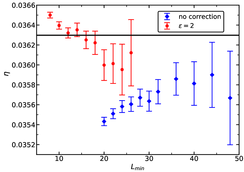
Figure 1: Results for the critical exponent $\eta$ obtained by fitting our numerical estimates of the magnetic susceptibility $\chi$ at $D=0.655$ and $\beta=0.387721735$ by using the ansätze (24,25). The solid line indicates the result obtained from conformal bootstrap $\eta=0.0362978(20)$, ref. Simmons-Duffin:2016wlq . All data with $L\geq L_{min}$ are taken into account in the fit.

Finally we check the possible effect of residual leading corrections to scaling at $D=0.655$. In ref. myBC , we conclude that compared with the Ising model on the simple cubic lattice, leading corrections to scaling are suppressed at least by a factor $1/30$. Based on that we have generated synthetic data by multiplying our data for $D=0.655$ by the factor $(1\pm[0.22/30]L^{-\omega})$, where the coefficient $0.22$ stems from the analysis for the Ising model discussed in appendix D. Using these synthetic data we have repeated the fits using the ansätze (24,25). In the case of the ansatz (25) for $L_{min}=16$ we find that the estimate of $\eta$ changes by $\pm 0.00023$. For the ansatz (24) and $L_{min}=36$ we find that the estimate of $\eta$ changes by $\pm 0.00026$.

Finally we consider the quantity $\chi_{imp}=U_{4}^{x}\chi$. The construction of such quantities is for example discussed in ref. ourdilute . The exponent $x$ is taken such that leading corrections to scaling in $U_{4}^{x}$ and $\chi$ cancel. Analyzing our data for the Ising model and the Blume-Capel model at $D=1.15$ we find $x=-1.4$, where the error is small enough to ensure a reduction of the amplitude of the leading correction to scaling by one order of magnitude. Fitting $\chi_{imp}$ with the ansatz (25) we find $\eta=0.03625(17)$ for $L_{min}=16$ and with the ansatz (24) we find $\eta=0.03588(30)$ for $L_{min}=36$. Note that in particular the result obtained with the ansatz (25) is in very good agreement with the conformal bootstrap.

V.2.2 The scaling behavior of the autocorrelation time

First we fitted the ratio $\tau_{M,C}/\tau_{HB,C}$ using the ansatz (23), where now the exponent $\epsilon$ is a free parameter. We get $\chi^{2}/$d.o.f. $=0.97$ taking all lattice sizes into account. We get $\epsilon=2.097(23)$, $2.167(44)$, $2.135(80)$, and $2.04(13)$, for $L_{min}=8$, $10$, $12$, and $14$, respectively, where all linear lattice sizes $L\geq L_{min}$ are taken into account.

We have fitted our results using the basic ansätze

$$\tau=a_{A}L^{z}$$ (26)

and

$$\tau=a_{A}L^{z}\;\;(1+c_{A}L^{-\epsilon})\;,$$ (27)

where $a_{A}$, $c_{A}$ and $z$ are the free parameters. The subscript $A$ denotes the algorithm that is used. We have fixed the correction exponent $\epsilon=2$. Replacing the $2$ by $2-\eta$ or $\omega_{NR}$ has only little effect on the results for $z$.

In a first series of fits we analyzed the data for the heat bath and the Metropolis updates separately. The results for the exponent $z$ are shown in figure 2. In the case of the heat bath algorithm and the ansatz (27) we find that $\chi^{2}/$d.o.f.$<1$ starting from $L_{min}=8$. In the case of the Metropolis algorithm and the ansatz (27) we get $\chi^{2}/$d.o.f.$=1.46$, $1.35$, and $1.20$ for $L_{min}=10$, $12$, and $14$. For larger $L_{min}$ it fluctuates at this level. In the case of the Metropolis algorithm and the ansatz (26) we have $\chi^{2}/$d.o.f.$=1.20$ for $L_{min}=20$. This is related with the fact that fits with the ansatz (27) give small values for the correction amplitude $c_{M}$. In the case of the heat bath algorithm and the ansatz (26) we find $\chi^{2}/$d.o.f.$=2.98$ for $L_{min}=20$, dropping below one at $L_{min}=28$.

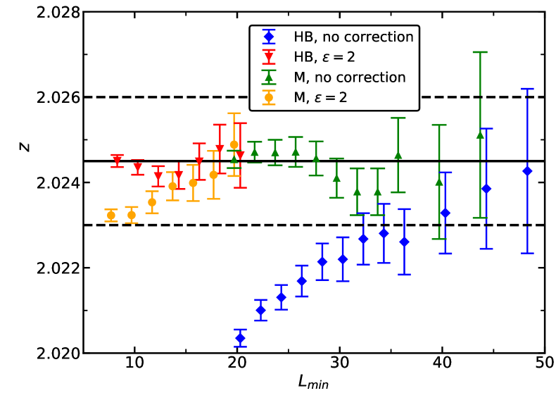
Figure 2: Results for the dynamic critical exponent $z$ obtained from fitting our numerical results for the integrated autocorrelation time of the magnetic susceptibility $\tau_{int,\chi}$ at $D=0.655$ and $\beta=0.387721735$ by using the ansätze (26,27). All data with $L\geq L_{min}$ are taken into account in the fit. In the caption, the Metropolis and the heat bath algorithm are indicated by M and HB, respectively. For better readability we have slightly shifted the values of $L_{min}$. The solid line gives the central value of our estimate $z=2.0245(15)$, while the dashed lines indicate the error.

Next we check the possible effect of residual leading corrections to scaling. To this end, we multiply our data for $\tau$ of the heat bath algorithm with $1\pm[0.43/30]L^{-\omega}$. For $L_{min}=16$ and the ansatz (27) the estimate of $z$ changes by $\pm 0.00045$. For $L_{min}=36$ and the ansatz (26) it changes by $\pm 0.00049$. To see what we would get for the Ising model, we multiplied the data with $1-0.43L^{-\omega}$. Fitting with the ansatz (26) we get $\chi^{2}/$d.o.f.$<1$ starting from $L_{min}=30$. For example for $L_{min}=32$ we get $z=2.0385(6)$. Note that $(2.0385-2.024)/0.0006\approx 24$.

We did not simulate the Ising model or the Blume-Capel model with our Metropolis algorithm, since it seems to be a safe guess that the effect of leading corrections is much the same as for the heat bath algorithm.

We also performed a joint fit of the Metropolis and the heat bath data using the ansatz (27), where $a_{M}$, $c_{M}$, $a_{HB}$, $c_{HB}$, and $z$ are the free parameters. For example we get $z=2.02424(30)$ for $L_{min}=16$. Note that $\chi^{2}/$d.o.f.$<1$ already for $L_{min}=12$.

Finally we fitted the improved autocorrelation time $\tau_{imp}=U_{4}^{x}\tau$, where $x=-3.1$ for the heat bath algorithm. Here we find $z=2.02462(46)$ for $L_{min}=16$.

Focusing on the fits with the ansatz (27) and $L_{min}=14$, $16$ and $18$ we arrive at the estimate

$$z=2.0245(15)\;\;.$$ (28)

The error bar covers all the fits that we performed with the ansatz (27) and $L_{min}=14$, $16$ and $18$. Also possible effects of residual leading corrections to scaling are taken into account. The error bar also covers the fits of the autocorrelation times for the Metropolis algorithm using the ansatz (26). In the case of the heat bath algorithm and the ansatz (26) at least the central values are covered for $L_{min}\geq 40$. Completely covering also the error bars of these fits, in particular in the light of the results for the exponent $\eta$ in the section above, seems to be too pessimistic. Since $\beta_{c}$ was determined in myBC using larger lattices and higher statistics than here, it seems safe to ignore the error induced by the uncertainty of the estimate of $\beta_{c}$.

VI Sudden quench from $T=0$ to criticality

We have simulated the Blume-Capel model at $D=0.655$ by using our Metropolis algorithm and the heat bath algorithm both with checkerboard ordering. At time $t=0$, we start with a fully magnetized configuration corresponding to zero temperature and perform a sudden quench to $\beta=0.387721735$, which is our estimate of the inverse of the critical temperature myBC . Updating all sites of the lattice once is taken as unit of time. In the analysis we focus for simplicity on the magnetization. In the thermodynamic limit, it behaves as

$$m(t)=a(t-t_{0})^{-\lambda_{m}}\;,$$ (29)

where $\lambda_{m}=\beta/\nu z$. See eq. (2) of ref. Ito93 and references therein. Note that $\beta/\nu=\Delta_{\sigma}=0.5181489(10)$ in three dimensions Simmons-Duffin:2016wlq . Eq. (29) is subject to leading corrections of the equilibrium universality class. Since we simulate an improved model, we ignore these corrections in our analysis. We only take explicitly into account analytic corrections that are expressed by $t_{0}$.

VI.1 Simulations using the Metropolis algorithm

Most of our simulations were performed using lattices of the linear size $L=300$. As a check of finite size effects, we performed simulation with $L=50$ and $100$ in addition. In the case of $L=50$ and $100$ we performed $2000\times 64$ runs and for $L=300$ we performed $4000\times 64$ runs. For $L=50$ we did run up to $t=1000$ and for $L=100$ and $300$ up to $t=4000$. Statistical errors are computed by using the jackknife method. Using the multispin coding technique, 64 runs are performed in parallel, partially sharing the same pseudo random number stream, possibly causing a statistical correlation. Therefore these runs are always put in the same jackknife bin, not to corrupt the estimate of the statistical error.

In figure 3 we plot ratios of the magnetization as a function of the Monte Carlo time $t$. We find that for $L=50$ the deviation from $L=300$ reaches a $3\sigma$ level for $t\gtrapprox 840$. For $L=100$ this is the case for $t\gtrapprox 3500$. In both cases we regard the magnetization for $L=300$ as approximation of the thermodynamic limit. From scaling we expect that the point of deviation from the thermodynamic limit by a certain fraction behaves as $t\propto L^{z}$. Therefore we conclude that for $L=300$ up to $t=4000$ deviations from the thermodynamic limit can be safely ignored at the level of our statistics. In the following only data obtained for $L=300$ are considered. In total, the simulations for $L=300$ took the equivalent of about 440 days on a single core of a Intel(R) Xeon(R) CPU E3-1225 v3 CPU.

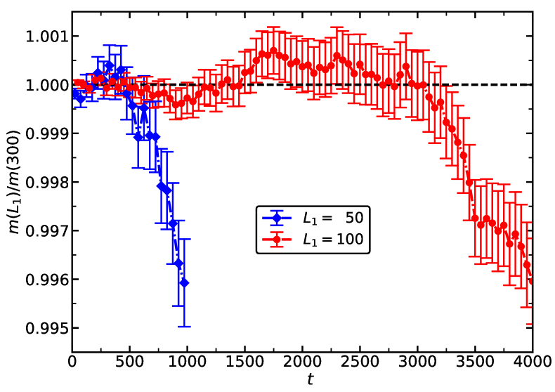
Figure 3: Simulations with the Metropolis algorithm. We plot the ratios $m_{L_{1}}(t)/m_{L_{2}}(t)$ for $L_{1}=50$ and $100$ and $L_{2}=300$ as a function of $t$. For the readability of the figure we only give a fraction of the $t$ values.

By construction the data for the magnetization at different values of $t$ are correlated. We tried to avoid fitting a large data set with correlations and keep the analysis simple. Our starting point is an effective exponent given by

$$z_{m,eff,t_{0}}(t)=-\Delta_{\sigma}\frac{\ln\left[(2t-t_{0})/(t-t_{0})\right]}{\ln\left[m(2t)/m(t)\right]}\;,$$ (30)

where $t_{0}$ remains a free parameter.

In a first step of the analysis we fix $t_{0}$ by requiring that $z_{m,eff,t_{0}}(t)$ has a minimal variance in the interval $t_{1}\leq t<t_{2}$: The average of $z_{m,eff,t_{0}}$ in the interval is denoted by

$$\bar{z}_{m,eff,t_{0}}(t_{1},t_{2})=\frac{1}{t_{2}-t_{1}}\sum_{t=t_{1}}^{t_{2}-1}z_{m,eff,t_{0}}(t)\;\;.$$ (31)

Then we minimize

$$\mbox{var}(z,t_{0},t_{1},t_{2})=\sum_{t=t_{1}}^{t_{2}-1}\left[z_{m,eff,t_{0}}(t)-\bar{z}_{m,eff,t_{0}}(t_{1},t_{2})\right]^{2}$$ (32)

with respect to $t_{0}$. The results of this analysis for $t_{2}=2t_{1}$ and various values of $t_{1}$ are given in table 3. With increasing $t_{1}$, the estimate of $t_{0}$ is increasing, while that of $z$ is decreasing. The corrections are compatible with $t_{1}^{-1}$ and $t_{1}^{-2}$, respectively. Fitting the results for $t_{1}\geq 60$, not taking into account the statistical correlations, we arrive at $z=2.0244(4)$ and $t_{0}=-2.13(10)$. As our preliminary estimate of this section we take

$$t_{0}=-2.1(2)\;\;,\;\;z=2.0245(10)\;\;,$$ (33)

which is compatible with both our extrapolation in $t_{1}$ and the result obtained for $t_{1}=160$.

Table 3: Simulations with the Metropolis algorithm for $L=300$. We give the results of minimizing the variance of $z_{m,eff,t_{0}}$ within the intervals $t_{1}\leq t<2t_{1}$, eq. (32), with respect to $t_{0}$.

$t_{1}$	$t_{0}$	$z$
20	-1.380(5)	2.04089(20)
30	-1.571(9)	2.03315(24)
40	-1.679(13)	2.03006(28)
60	-1.838(25)	2.02677(36)
80	-1.944(38)	2.02524(42)
120	-1.95(8)	2.02523(54)
160	-2.01(12)	2.02481(65)
240	-2.01(24)	2.02470(87)

As a check, in figure 4, we plot $z_{m,eff,t_{0}}(t)$ for $t_{0}=3.1$ for the full range of $t$ that we have simulated.

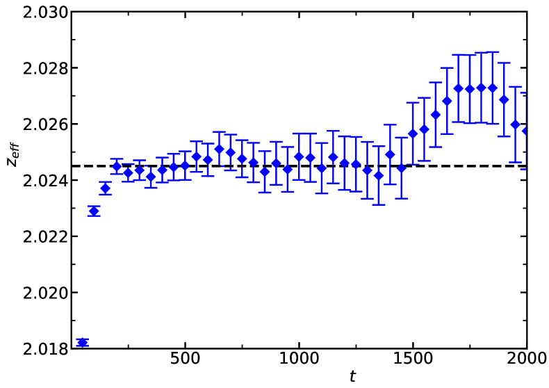
Figure 4: Simulations with the Metropolis algorithm. The effective exponent $z_{eff}$ as defined by eq. (30) for $L=300$ and $t_{0}=-2.1$. The dashed line indicates the preliminary result $z=2.0245$ of this section.

VI.2 Simulations using the heat bath algorithm algorithm

In this section we discuss simulations similar to those of the previous one, replacing the Metropolis by the heat bath algorithm. Details of the simulation program are discussed in the appendix A. Based on the results obtained above, we simulated lattices of the linear size $L=300$. We run the simulations up to $t=2000$. We performed 10000 runs with 32 replicas each. In total, these simulations took the equivalent of about 370 days on a single core of a Intel(R) Xeon(R) CPU E3-1225 v3 CPU.

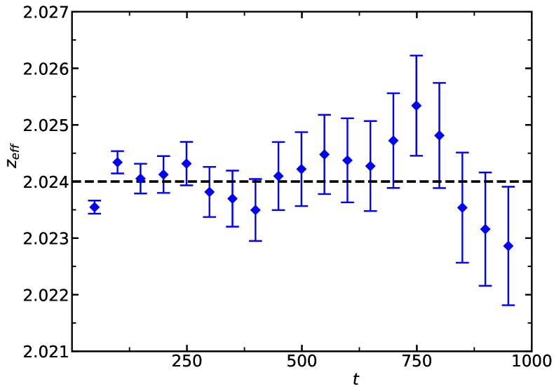
Figure 5: Simulations with the heat bath algorithm. The effective exponent $z_{eff}$ as defined by eq. (30) for $L=300$ and $t_{0}=0$. The dashed line indicates the preliminary result $z=2.024$ of this section.

First we compared the relaxation times of the heat bath and the Metropolis algorithm. We computed the ratio $t_{M}(m)/t_{HB}(m)$, where $t_{M}(m)$ and $t_{HB}(m)$ are the times needed by the Metropolis and the heat bath algorithm to reach a certain value $m$ of the magnetization. Using a linear extrapolation in $t$ we arrive at the estimate $t_{M}/t_{B}=1.3304(8)$ for the limit $t_{B},t_{M}\rightarrow\infty$. This ratio is in good agreement with the ratio of autocorrelation times, reported in table 2 above.

Table 4: Same as table 3 but for the heat bath instead of the Metropolis algorithm.

$t_{1}$	$t_{0}$	$z$
15	0.0148(25)	2.02379(14)
20	0.0219(49)	2.02421(18)
30	0.031(8)	2.02459(24)
40	0.010(13)	2.02395(29)
60	-0.003(27)	2.02364(40)
80	0.026(44)	2.02409(49)
120	0.032(89)	2.02420(66)
160	0.09(15)	2.02467(82)

In table 4 we report our result for $z$ and $t_{0}$ obtained from the minimization procedure discussed above for the Metropolis algorithm. Compared with the estimates reported in table 3 for the Metropolis algorithm, the estimates for $z$ and $t_{0}$ show very little dependence on the range in $t$. Therefore we abstain from extrapolating the results. Based on the result for $t_{1}=40$ we take $z=2.0240(8)$ and $t_{0}=0.0(1)$ as our preliminary result. The error bars are taken such that they include all estimates with their error bars up to $t_{1}=120$. As a check, in figure 5 we give $z_{eff}$, eq. (30), for $t_{0}=0$.

VII Summary and Conclusions

We have studied a purely dissipative relaxational dynamics for the improved Blume-Capel model on the simple cubic lattice. This model shares the universality class of the three-dimensional Ising model. Improved means that the parameter $D$ of the model is chosen such that the amplitude of leading corrections to scaling is strongly suppressed. In particular, since we have to face critical slowing down when studying a relaxational process, it is important to use an improved model, since here already from relatively small lattices reliable results can be obtained.

The numerical results for the dynamic critical exponent $z$ given in the literature vary considerably. In particular there is a clear discrepancy between most of the results obtained by the simulation of the Ising model and field theoretic results. Only a previous simulation of the Blume-Capel model gives a result that is consistent with field theory.

We have computed the dynamic critical exponent by using two different approaches. As our final estimate we quote $z=2.0245(15)$ obtained from the finite size scaling analysis of equilibrium autocorrelation times at the critical point. The results that we obtain from the sudden quench of a fully magnetized configuration to criticality are fully consistent with this estimate.

Note that our estimate of the dynamic critical exponent is in nice agreement with recent results obtained with the functional renormalization group method Me15 ; FRG . The same holds for the analysis of the four-loop $\epsilon$-expansion Ad17 presented here in appendix C.

VIII Acknowledgement

I like to thank M. V. Kompaniets for very helpful correspondence. This work was supported by the Deutsche Forschungsgemeinschaft (DFG) under grant No HA 3150/5-1.

Appendix A Parallel program using SSE2 intrinsics and shared use of random numbers

In a second stage of the project we made an effort to speed up our simulation program for the heat bath algorithm. To this end we have chosen an approach that is less involved than the multispin coding technique that builds on bitwise operations. Here we exploited the SSE2 instruction set of x86 CPUs. These were accessed by using SSE2 intrinsics. SSE2 instructions act on several variables that are packed into 128 bit units in parallel. In our case we store a single spin as a 8 bit char variable, of which 16 are packed into a 128 bit unit. To this end, we run 16 replicas of the system in parallel. For each site $x$ we pack the 16 spins $s_{x}^{(j)}$, where the upper index labels the replica, into a __m128i variable. Computing the sum of the neighbors for the update and the measurement of the magnetization are done in parallel for the 16 replicas. The actual heat bath update is still done one by one.

Since the generation of a pseudo random number is relatively expensive, it is a natural question, whether we can use the same stream of random numbers for several replicas. One simple idea is to take a stream $r_{i}^{(0)}$ of random numbers that are uniformly distributed in $[0,1)$ and then use the family

$$r_{i}^{(j)}=\mbox{frac}(r_{i}^{(0)}+j/N)\;,$$ (34)

where $j=0,1,2,...,N-1$ for the simulation of $N$ replicas and frac is the fractional part of a real number. This way, all replicas are simulated by using a well behaved pseudo random number. However a statistical correlation among the replicas arised. We computed statistical errors by using the jackknife method. Not to corrupt the estimate of the statistical error, correlated replicas are always put in the same bin. For the simplicity of the program, we did not measure the correlation of the runs that share the family of random numbers. Instead, for a few lattice sizes we performed runs, where each replica has its own pseudo random number. Then we compared the statistical errors obtained for equal statistics. It turns out that in the case of the simulations in equilibrium at $\beta_{c}$ we see virtually no effect on the statistical error up to about $N=4$. For larger values of $N$ we see a gradual increase of the relative statistical error with increasing $N$. In our simulations reported in section V.2 we use $N=4$ throughout.

In the case of the sudden quench from zero temperature to the critical one we also experimented with eq. (34). For small $N$ we even find a small reduction of the statistical error compared with independent random numbers.

However it turned out that an even larger variance reduction can be obtained by sharing the random number in a different way. P. Grassberger private pointed out that the heat bath algorithm applied to the Blume-Capel model fulfills the property of ”monotonicity” Con ; See also the introduction of ref. Grassberger .

Two replica $A$ and $B$ of the system are simulated. At time $t=0$

$$s_{x}^{(A)}\geq s_{x}^{(B)}$$ (35)

holds for all sites $x$, where the upper index denotes the replica. These two replicas are simulated by running through the sites in the same order, using exactly the same stream of random numbers for both systems. Then the condition (35) is preserved by the update. This property is actually easy to prove. Let us start with the precise definition of the heat bath update: At the site $x$ the new value of the spin $s_{x}$ is chosen with the probabilities

$$p(-1)=\exp(-D-\beta S_{x})/z\;\;,\;p(0)=1/z\;\;,\;p(0)=\exp(-D+\beta S_{x})/z$$ (36)

with $z=\exp(-D-\beta S_{x})+1+\exp(-D+\beta S_{x})$ and $S_{x}=\sum_{y.nn.x}s_{y}$ is the sum of the nearest neighbors. This is implemented in the following way: First a uniformly distributed random number $r\in[0,1)$ is drawn. Then $s_{x}^{\prime}=-1$ is taken if $r<p(-1)$, $s_{x}^{\prime}=0$, if $p(-1)\leq r<p(-1)+p(0)$ and $s_{x}^{\prime}=1$, if $p(-1)+p(0)\leq r$. Since $p(-1)$ is monotonically decreasing with increasing $S_{x}$, it follows for any given $r$ that if $S_{x}^{(A)}\geq S_{x}^{(B)}$ then $s_{x}^{\prime(A)}\geq s_{x}^{\prime(B)}$. Hence starting with eq. (35) this property is preserved throughout the simulation. This property allows for a variance reduction in the measurement of time dependent magnetization densities and variances thereof. For details see ref. Grassberger .

In our case, we run two replicas initialized with positive and negative magnetization, using the same stream of random numbers. The estimator of the magnetization is

$$m_{I}(t)=\frac{m_{+}(t)-m_{-}(t)}{2}\;,$$ (37)

where the subscript $\pm$ indicates the initialization of the system. By construction $m_{I}(t)\geq 0$ for all $t$. Hence at least for large $t$, when the system is close to equilibrium, there should be a reduction of the variance. The numerical experiment shows that this is also the case for times $t$ relevant in our study. We compare with two systems running with independent random number streams. We find that initially the gain increases rapidly from about 1.3 for the first measurement to about 2.2 at $t\approx 30$. Then it slowly increases up to about 2.5 at $t=2000$.

We also tried to combine this idea with eq. (34). Unfortunately we see a counteracting effect. Taking also into account the CPU time needed to generate a random number, we have chosen $N=2$ for our production runs. In our SSE2 program we have simulated in parallel 16 replica with all spin up and 16 replica with all spin down initialization using 8 independent streams of pseudo random numbers.

The general ideas on the reuse of random numbers and variance reduction are widely used. One can easily convince oneself by typing the keywords ”common random numbers” or ”antithetic variates” in a search engine or have a look at a text book on Monte Carlo methods such as ref. Kroese for example.

Appendix B The two-dimensional Ising model

In the analysis of the four-loop $\epsilon$-expansion result Ad17 we shall use the numerical estimate of $z$ for the universality class of the two-dimensional Ising model as boundary condition. The most precise estimates given in the literature are $z=2.1665(12)$ NiBl96 and $z=2.1667(5)$ NiBl00 . These estimates were obtained from the analysis of very accurate estimates of $\tau_{exp}$ obtained for linear lattices sizes $L\leq 15$. The accuracy of the estimates of $z$ relies on the correctness of the ansatz for corrections to scaling. The leading correction is proportional to $L^{-2}$. In refs. NiBl96 and NiBl00 also subleading corrections had to be taken into account.

Here we performed simulations of the two-dimensional Ising model on the square lattice exactly at the critical temperature. We determine the integrated autocorrelation time of the magnetic susceptibility in exactly the same way as in section V. We performed simulations for 27 different linear lattice sizes from $L=8$ up to $120$.

We fitted our data using the ansätze

$$\tau = cL^{z}\;,$$ (38)

$$\tau = aL^{z}\;(1+bL^{-2})\;,$$ (39)

$$\tau = aL^{z}\;(1+bL^{-2}+cL^{-4})\;.$$ (40)

For example using the ansatz (40) we get $\chi^{2}/$d.o.f.$=1.13$, $a=0.06417(4)$, $b=6.42(5)$, $c=-17.4(2.9)$ and $z=2.1663(2)$, when including all lattice sizes $L\geq 10$ in the analysis. Using the ansatz (39) we get $\chi^{2}/$d.o.f.$=1.00$, $a=0.06397(9)$, $b=6.89(20)$ and $z=2.1670(4)$ taking into account all lattice sizes $L\geq 16$. Using the ansatz without corrections we get $\chi^{2}/$d.o.f.$=0.82$, $a=0.0644(2)$ and $z=2.1657(7)$ using all data with $L\geq 56$. Assessing all fits that we performed, we arrive at the estimate $z=2.167(2)$, confirming the results of refs. NiBl96 ; NiBl00 .

Appendix C Analyzing the field theoretic results

Here we make an attempt to extract a number for $z$ for three dimensions by using the four-loop $\epsilon$-expansion result Ad17 . For the Ising universality class the authors give

$$z=2+0.0134461561\epsilon^{2}+0.011036273(10)\epsilon^{3}-0.0055791(5)\epsilon^{4}+O(\epsilon^{5})\;.$$ (41)

Reexpressing this result by using eq. (3) we get

$$c=0.72609243\;\left(1-0.188484\epsilon+0.22506\epsilon^{2}+...\right)\;.$$ (42)

The $[1/1]$ Padé approximation is

$$c\approx 0.72609243\;\;\frac{1+1.00557\epsilon}{1+1.19405\epsilon}\;.$$ (43)

Inserting $\epsilon=1$ and $2$, using $\eta=0.0362978(20)$ Simmons-Duffin:2016wlq and $\eta=1/4$ we get $z=2.0241$ and $2.1613$, respectively. Enforcing $z=2.167$ in two dimensions, we arrive at

$$c\approx 0.72609243\;\;\frac{1+0.82727\epsilon+0.03361\epsilon^{2}}{1+1.01575\epsilon}\;$$ (44)

resulting in $z=2.0243$ for three dimensions.

Bausch et al. Bausch81 studied the dynamics of an interface in $1+\epsilon^{\prime}$ dimensions. They arrive at $z=2+\epsilon^{\prime}-\frac{1}{2}\epsilon^{\prime 2}+...$ for the dynamic critical exponent. They give an interpolation of their result and the two-loop $\epsilon$-expansion, eq. (9) of Bausch81 . Inserting $d=2$ and $3$, one gets $z=2.126$ and $2.019$, respectively.

Extending the approach of Bausch81 by using the result of Ad17 we arrive at

$$z-2\approx\frac{(0.0348932-0.0076607d)\;(d-1)\;(4-d)^{2}}{1-1.532616d+0.910303d^{2}-0.132595d^{3}}\;.$$ (45)

Inserting $d=2$ and $3$, one gets $z=2.1519$ and $2.0235$, respectively. Enforcing $z=2.167$ in two dimensions, we arrive at

$$z-2\approx\frac{(0.0419521-0.0131387d+0.00083183d^{2})\;(d-1)\;(4-d)^{2}}{1-1.443329d+0.834824d^{2}-0.124687d^{3}}$$ (46)

giving $z=2.0245$ in three dimensions.

The four-loop result for the expansion in three dimensions fixed is Prud97 :

$$z-2=0.008399g^{2}-0.000045g^{3}-0.020423g^{4}\;.$$ (47)

Following the idea of ref. HaHoMa72 we might analyze

$$\frac{z-2}{\eta}=0.765359(1-0.088666g+2.275305g^{2})\;,$$ (48)

where the series for $\eta$ is taken from ref. gstar , eq. (2.4). We arriving at the $[1/1]$ Padé approximation

$$\frac{z-2}{\eta}\approx 0.765359\frac{1+25.5729g}{1+25.6615g}\;.$$ (49)

Inserting the fixed point value $g^{*}=1.4299$, eq. (22) of ref. Prud97 , and $\eta=0.0362978(20)$, we get $z=2.0277$, which is considerably larger than the value obtained by the Padé approximation for $z-2$ itself.

We find that the estimates obtained by different resummation schemes scatter less for the four-loop $\epsilon$-expansion than for the four-loop expansion in three dimensions fixed. As our final estimate we take

$$z=2.0243$$ (50)

from eq. (44). Assigning an error bar is a difficult task. Comparing the different estimates eqs. (43,44,45,46), it should be at most a one in the third decimal place.

Appendix D Leading corrections to scaling

In order to study the effect of leading corrections to scaling on the autocorrelation times, we simulated the Ising model and the Blume-Capel model at $D=1.15$ at the estimates of the inverse critical temperature $\beta_{c}=0.221654626(5)$, ref. pushing , and $0.4756110(2)$, ref. myBC , respectively. We simulated the linear lattice sizes $L=8,10,12,...,24$ by using the heat bath algorithm with checkerboard decomposition. In order to demonstrate the size of corrections to scaling, we plot in figure 6 the Binder cumulant $U_{4}=\frac{\langle m^{4}\rangle}{\langle m^{2}\rangle^{2}}$ for the Ising model and the Blume-Capel model at $D=0.655$ and $1.15$. At the critical point it behaves as

$$U_{4}(L,D)=U_{4}^{*}+a(D)L^{-\omega}+b\;a^{2}(D)L^{-2\omega}+...+c(D)L^{-\omega^{\prime}}+...\;,$$ (51)

where the term $c(D)L^{-\omega^{\prime}}$ represents subleading corrections. Almost degenerate subleading correction exponents are $2-\eta=1.9637022(20)$ due to the analytic background in the magnetic susceptibility and $\omega_{NR}=2.022665(28)$ Simmons-Duffin:2016wlq . Estimates of the fixed point value are $U_{4}^{*}=1.6036(1)$, ref. myBC and $1.60356(15)$, ref. pushing .

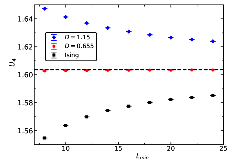
Figure 6: We plot the Binder cumulant $U_{4}=\frac{\langle m^{4}\rangle}{\langle m^{2}\rangle^{2}}$ at the critical temperature for the Ising model and the Blume-Capel model at $D=0.655$ and $1.15$. Note that the error bars are clearly smaller than the symbol size. The dashed line gives the estimate $U_{4}^{*}=1.6036(1)$ of the fixed point value myBC .

Fitting the data for $U_{4}$ at $D=0.655$ confirms that the amplitude of leading corrections vanishes at the level of our numerical precision. Next we analyzed the ratios

$$r_{U_{4}}(D,L)=\frac{U_{4}(D,L)}{U_{4}(D=0.655,L)}$$ (52)

using the ansätze

$$r_{U_{4}}(D,L)=1+a_{U}(D)L^{-\omega}$$ (53)

and

$$r_{U_{4}}(D,L)=1+a_{U}(D)L^{-\omega}+b_{U}(D)L^{-2}\;,$$ (54)

where we have fixed $\omega=0.82968$.

For the Ising model we find using the ansatz (54), including all data $a_{U}(-\infty)=-0.1530(5)$, $b_{U}(-\infty)=-0.178(8)$ and $\chi^{2}/$d.o.f.$=0.68$. Instead using the ansatz (53) we get $a_{U}(-\infty)=-0.1577(5)$ and $\chi^{2}/$d.o.f.$=0.8$ when including all lattice sizes with $L\geq 20$. We conclude $a_{U}(-\infty)=-0.155(4)$.

For $D=1.15$, using the ansatz (54), including all data with $L\geq 10$ we get $a_{U}(1.15)=0.1839(5)$, $b_{U}(1.15)=-0.328(9)$ and $\chi^{2}/$d.o.f.$=1.22$. Instead, using the ansatz (53) we get $a_{U}(1.15)=0.1760(8)$ and $\chi^{2}/$d.o.f.$=2.83$ when including all lattice sizes with $L\geq 20$. We conclude $a_{U}(1.15)=0.180(5)$.

Next we analyzed ratios of susceptibilities

$$r_{\chi}(D,L)=\frac{\chi(D,L)}{\chi(D=0.655,L)}\;,$$ (55)

where the powerlike divergence $\chi\propto L^{2-\eta}$ cancels. We fitted these ratios with

$$r_{\chi}(D,L)=c_{\chi}(D)(1+a_{\chi}(D)L^{-\omega})$$ (56)

and as check

$$r_{\chi}(D,L)=c_{\chi}(D)\;(1+a_{\chi}(D)L^{-\omega}+b_{\chi}(D)L^{-2})\;,$$ (57)

where we have fixed $\omega=0.82968$. In the case of the Ising model we get $\chi^{2}/$d.o.f.$=0.84$ and $a_{\chi}(-\infty)=-0.2211(7)$ including all data with $L\geq 10$ using the ansatz (56). Instead, using the ansatz (57) we get $\chi^{2}/$d.o.f.$=1.00$, $a_{\chi}(-\infty)=-0.220(6)$ and $b_{\chi}(-\infty)=-0.01(5)$, taking into account $L\geq 10$. We take $a_{\chi}(-\infty)=-0.220(6)$ as our final result.

In the case of $D=1.15$ we get by using the ansatz (56) taking into account all data for $L\geq 12$ the result $\chi^{2}/$d.o.f.$=1.13$ and $a_{\chi}(1.15)=0.2483(15)$. Instead, using the ansatz (57) we get $\chi^{2}/$d.o.f.$=0.70$, $a_{\chi}(1.15)=0.262(7)$ and $b_{\chi}(1.15)=-0.13(6)$, taking into account $L\geq 10$. As our final estimate we take $a_{\chi}(1.15)=0.255(14)$ that covers both fits, including their error bars.

Finally we computed ratios of autocorrelation times

$$r_{\tau}(D,L)=\frac{\tau(D,L)}{\tau(D=0.655,L)}\;,$$ (58)

where the power divergence $\propto L^{z}$ should cancel and, hopefully also corrections due to the breaking of the Galilean symmetries by the lattice to a large extend. We fitted these ratios by using the ansätze

$$r_{\tau}(D,L)=c_{\tau}(D)\;(1+a_{\tau}(D)L^{-\omega})$$ (59)

and as check

$$r_{\tau}(D,L)=c_{\tau}(D)\;(1+a_{\tau}(D)L^{-\omega}+b_{\tau}(D)L^{-2})\;,$$ (60)

where we have fixed $\omega=0.82968$.

In the case of the Ising model we get from (59), including all data with $L\geq 10$ the estimate $a_{\tau}(-\infty)=-0.452(2)$ and $\chi^{2}/$d.o.f.$=1.00$. Fitting with the ansatz (60), $b_{\tau}(D)$ is compatible with zero and $a_{\tau}(-\infty)=-0.43(2)$. We conclude $a_{\tau}(-\infty)=-0.44(3)$. For $D=1.15$ we get, fitting all data with $L\geq 14$ by using the ansatz (59) the estimate $a_{\tau}(1.15)=0.602(10)$ and $\chi^{2}/$d.o.f.$=1.14$. Fitting with the ansatz (60), using all data we get $a_{\tau}(1.15)=0.631(13)$, $b_{\tau}(1.15)=-0.49(8)$ and $\chi^{2}/$d.o.f.$=1.86$. We conclude $a_{\tau}(1.15)=0.62(3)$. These fits support the hypothesis that $z$ does not depend on $D$, and the differences can be explained by corrections.

According to the renormalization group, leading corrections to scaling are caused by a unique scaling field. Therefore, the ratios of correction amplitudes for different quantities assume universal values. In particular, for the improved model the amplitude of leading corrections vanishes for all quantities.

For the susceptibility and the Binder cumulant we get $a_{\chi}(-\infty)/a_{U}(-\infty)=$
$[-0.220(6)]/[-0.155(4)]=1.42(7)$ and $a_{\chi}(1.15)/a_{U}(1.15)=[0.255(14)]/[0.180(5)]=1.42(9)$. We conclude $a_{\chi}/a_{U}=1.42(9)$.

For the autocorrelation time and the Binder cumulant we get

$$\frac{a_{\tau}(-\infty)}{a_{U}(-\infty)}=\frac{-0.44(3)}{-0.155(4)}=2.84(30)$$ (61)

and

$$\frac{a_{\tau}(1.15)}{a_{U}(1.15)}=\frac{0.61(3)}{0.180(5)}=3.39(25)\;,$$ (62)

confirming the universality of the ratio of correction amplitudes. As our final result we take $a_{\tau}/a_{U}=3.1(6)$.

Note that the amplitude of the leading correction is relatively large for the autocorrelation time compared with the Binder cumulant and the magnetic susceptibility. This might explain the wide spread of the estimates of $z$ obtained from simulations of the three-dimensional Ising model, when the leading correction to scaling is not explicitly taken into account in the analysis.