Unexpected gap creating two peaks in the periods of planets of metal-rich sunlike single stars

Abstract

The pileup of planets at periods of roughly one year and beyond is actually a bimodal peak with a wide, sharp gap splitting the peak of the pileup in a major population of large planets. Consisting of nearly 40% of planets with periods past 200 days, the periods of the planets of metal-rich stars like the sun in surface gravity which do not have a stellar companion show two strong peaks separated by a sparsely populated region. Monte Carlo tests show that this structure is unlikely to occur in random distributions, and a comparison with objects from all the other populations show that this feature is unlikely to be due to observational effects. The peaks have their highest density next to the gap. These two peaks are most strongly seen in single-planet systems, though the gap persists in multiple planet systems. These features are likely characteristic of planets with masses not too much lower than Jupiter, and perhaps not too much higher. The presence of well-defined features in the period distribution show that planet formation may be much more uniform than previously expected.

(2019), Unexpected gap creating two peaks in the periods of planets of metal-rich sunlike single stars, A.N., 2018;00:1–x.

1 Introduction

Planets form beyond a distance where materials can condense, so it is expected in the counts of exoplanets by log period there will be a main pileup beyond a range of low counts. The observed pileup in the log period counts of exoplanets at periods longer than a few hundred days is expected, but we report that for the planets of single stars like the sun in surface gravity and have similar or higher metallcity than the sun (“rSLSS” planets), this pileup is in fact split into two pileups in log period, with a sizable gap separating two peaks. This bimodal distribution of the pileup in such a significant fraction of planets is completely unexpected.

It is not surprising that the planets of stars that are more metal rich than the sun have a different distribution than those of stars that are relatively metal poor. One of the earliest properties found for stars hosting giant planets was the “planet-metallicity” correlation, that stars with higher iron abundance are more likely to host planets (Gonzalez, 1997; Santos ., 2003; Fischer  Valenti, 2005; Udry  Santos, 2007). The finding that planets of stars that are more metal-rich than the sun are in higher eccentricity orbits than are those planets associated with stars poorer in metals has been interpreted to mean that these two groups of objects represent two separate populations (Dawson  Murray-Clay, 2013; Taylor, 2012, 2013).

In this work we present the structure in the period distribution of these rSLSS objects. We will address the eccentricities of these objects in the context of the regions presented here in the next work.

We begin, in Section 2, by describing the main pileups of the main populations of “objects”, where “objects” refers to the set of parameters describing one planet, its orbit, and host star. The unlikelihood of the gap is explained here. In Section 3 we further divide the population with the two peaks separated by a gap, finding a subpopulation that shows the two peaks more distinctly. The lack of a peak in the other main populations is shown in Section 4, followed by demonstrations that the gap is unlikely in Section 5. We conclude by demonstrating how these features show that planet formation produces a surprising uniformity of results in a large population of large planets.

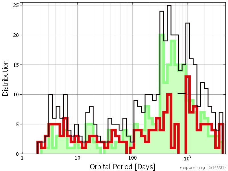
Figure 1: A histogram of all objects (black) shows the main pileup peaking at periods of between 300 and less than 1000 days but have a notch giving a hint of bimodal constituent. Also shown are the rSLSS objects (red) which have the bimodal peak, and the sum of all others (green, filled), which have a single peak. The width of the deep gap in log period space is shown as the horizontal black line.

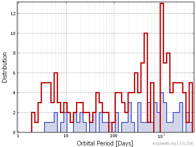
Figure 2: The distribution of periods of the 243 planets of single sunlike stars, with objects of 180 iron-rich stars shown in red (not filled) and planets of 63 iron-poor stars in blue (filled). The bins have been placed to fit four bins in the boundary of a gap from periods of 493.7 to 923.8 days. There is a deep gap of zero planets from 653.22 to 923.8 day periods, which is a little larger than the last two bins in the gap, that has zero planets.

2 Selections, one with a Gap

2.1 Discovery of a low density region

The peak-gap-peak feature was discovered while investigating how long in period the correlation of eccentricity with metallicity remained a correlation. It had been found at short periods, less than 100 days, (Dawson  Murray-Clay, 2013; Taylor, 2012) that the eccentricities of sunlike (SL) objects more metal rich that the sun (rSL) tended higher than the eccentricities of metal poor sunlike objects (pSL). Later work (Taylor, 2013) found that binary stars (BS) have higher eccentricities than single stars (SS), so Taylor (2013) subsequently focused on sunlike single stars (SLSS). While this pattern appears to continue to periods above 100 days, that is the means of the eccentricies of rSLSS objects are higher than those of pSLSS objects, it was found that at periods above 500 days there was a range where the eccentricities of pSLSS objects peaked, having some of the highest eccentricities. (The statistical significance of these eccentricity features is the subject of the next paper.) It was found, however, that in much of the period range of the peak pSLSS eccentricities that there are suddenly too few rSLSS objects to easily compare eccentricities. Not only do we now find only six rSLSS objects with periods from 493.7 to 923.8 days, we find zero rSLSS objects with periods in between the periods of 653.8 to 923.8 days. Starting at the period of 923.8 days, we find the highest density of of rSLSS objects’ periods per log period than anywhere in the period distribution so far measured.

2.2 Data source and selections

We use data downloaded from exoplanets.org (Han ., 2014) on 2017 January 31, which includes 434 total objects found by the radial velocity (RV) before 2016 at all periods up to 5000 days. We follow the convention of these planet parameters catalogs to refer to the combined set of data for each planet, including data on the orbit and host star, an “object”. We limit our study to only those objects with periods up to 5000 days day due to there being less data on objects with longer periods. The binned counts of these object’s periods is histogrammed in Figure 1, (black bins).

We study this “region of interest” (ROI) from 100 to 5000 day periods (1.7 in log period) that contains the main pileup of most of the planets, in which there are 313 objects. We choose this ROI to include periods longer than the shorter period “valley” region which has been characterized as having a paucity of objects (DM13) that goes up to 100 or 200 day periods .

We find new, unexpected features in the rSLSS selection of these objects, for planets of metal-rich sunlike stars, or “rSLSS” objects, where the “metallicity” of an object is that of the star.

We go through the steps we use to get to 113 rSLSS objects out of the 313 objects within the ROI that we divide from the “other” 198 objects hosted by stars with other parameters as explained below using Table 1:

We note that the sensitivity of RV observations only goes down to a rough minimum in projected planet mass, “$m$sin$i$”, and this minimum planet mass rises by period.

We divide the 434 objects by whether or not their stars’ surface gravity is equal to or above log $g$ of 4. This yields 190 objects hosted by stars with higher surface gravity that we call “sunlike” (SL) objects, after removing 123 low surface gravity (LSG) objects. We then divide these 190 SL objects into 156 single-star (SLSS) and 34 binary-star (SLBS) objects depending on whether the star has one or more stellar companions. We further divide the 156 SLSS objects into 41 “pSLSS” objects where the star is metal-poor and 115 “rSLSS” objects where the star is metal-rich relative to the sun. Lower-case abbreviations are used to delineate selections within SLSS (or SLBS) objects. The distribution of counts of rSLSS and pSLSS objects are compared in Figure 2. To keep the sample from having objects too far apart in effective temperature $T_{eff}$, and to be consistent with similar work, we apply a limit requiring objects have $T_{eff}$ in the range of 4500 to 6500 K, which eliminates two objects from our rSLSS selection. We cut these even though they both have periods within each of the two peaks presented here, such that their inclusion would strengthen the case for there being two peaks. This produces a sample of 113 rSLSS objects in the ROI, which are shown in red in Figure 1 and subsequent histograms. The mean density of rSLSS objects in the ROI is then 18.1 objects per gap-width, so the count of six objects in the gap is 0.33 of the mean ROI density, which we show is significantly low. In Figure 1 we use bins of one-quarter gap-width to show how the highest densities in the ROI are right next to the gap; here, the mean density per quarter-gap-width bin is 4.5 objects. We compare the distribution of the log periods of the rSLSS objects with the log periods of the 198 “other” objects, shown in green in Figure 1, consisting of 41 pSLSS, 34 SLBS, and 123 LSG objects.

The gap and two peaks can also be seen when we show the metallicity [Fe/H] versus the log period in Figure 3. For perspective, we show a more full region, though this does make the gap region appear smaller than if the figure zoomed in to the gap region. This figure shows a “gap” region in period with few SLSS objects (filled circles) with [Fe/H] above the dividing line that for simplicity we set at an [Fe/H] of zero, but the line actually would be better to be drawn at [Fe/H] of -0.03. Yet in this period region there is no reduction in SLSS objects with [Fe/H] below -0.03 or in LSG objects (green crosses), and only a possible small reduction in BS objects (red unfilled circles).

Table 1: Boundaries, counts, and densities of selections in the full ROI followed by the short period peak (SPP), the (shallow) gap between the peaks, and the long period peak (LPP). The counts are given, followed by the counts divided by how many gap-sized bins the range covers, which is a measure of the density of counts.

Regions	ROI	SP Tail	SP Peak	Gap	LP Peak	LP Tail
Start of period, days	100	100	$263.8$	493.7	923.8	1728.6
End of period, days	5000	263.8	$493.7$	923.8	1728.6	5000.0
Width of region, in log period	1.70	0.42	$0.27$	0.27	0.27	0.46
Fraction of ROI width	1.00	0.25	$0.16$	0.16	0.16	0.27
Width relative to gap	6.24	1.55	$1.00$	1.00	1.00	1.70
$m$sin$i$ limited loner rSLSS counts	56	7	$21$	0	19	9
Density in Counts per gap binwidth	9.0	4.5	$21.0$	0.0	19.0	5.3
No low $m$sin$i$ loner rSLSS counts	61	8	$21$	1	19	12
Density in Counts per gap binwidth	9.8	5.2	$21.0$	1.0	19.0	7.1
No high $m$sin$i$ loner rSLSS counts	58	8	$21$	1	19	9
Density in Counts per gap binwidth	9.3	5.2	$21.0$	1.0	19.0	5.3
Multiple rSLSS counts	50	13	$6$	4	13	14
Density in Counts per gap binwidth	8.0	8.4	$6.0$	4.0	13.0	8.3
Loner rSLSS counts	63	9	$21$	2	19	12
Density in Counts per gap binwidth	10.1	5.8	$21.0$	2.0	19.0	7.1
rSLSS counts	113	22	$27$	6	32	26
Density in Counts per gap binwidth	18.1	14.2	$27.0$	6.0	32.0	15.3
pSLSS counts	41	8	$5$	9	9	10
Density in Counts per gap binwidth	6.6	5.2	$5.0$	9.0	9.0	5.9
rSLBS counts	27	5	$7$	5	6	4
Density in Counts per gap binwidth	4.3	3.2	$7.0$	5.0	6.0	2.4
pSLBS counts	7	0	$0$	3	3	1
Density in Counts per gap binwidth	1.1	0.0	$0.0$	3.0	3.0	0.6
LSG counts	123	18	$39$	46	11	9
Density in Counts per gap binwidth	19.7	11.6	$39.0$	46.0	11.0	5.3

Source: exoplanets.org, Han . (2014), downloaded 2016 January 31.

2.3 One large selection has a gap not present in other selections

We compare the distribution of counts per log period of rSLSS objects with the distribution of other objects in Figure 1 to show (Section 4) that other selections have a single pileup, the rSLSS population has a bimodal pileup separated into two peaks by a gap covering the period range from 493.7 to 923.8 day periods, which is 0.272 in log period or 0.16 of the ROI. We find the gap-width to be a useful unit to use to compare the density per log period of the peaks, since the ROI is 6.24 gap-widths wide. The mean density of the 113 rSLSS objects is 18.1 objects per gap-width, so the six objects in the gap give it a density of only 0.33 of this mean. There are 49 (58) rSLSS objects in the ROI with periods shorter (longer) than the gap, a period range from 100 to 493.7 (923.8 to 5000) days that in log period covers 2.55 (2.70) gap-widths, which we call the short- (long-) periods side, [SPS (LPS)].

Counts of how many objects are in the main parts of the two peaks are given in Table 1, where we delineate both of the two regions at both sides of the gap into one gap-width peaks, leaving tails of 1.55 and 1.70 gap-widths on the SPS and LPS sides, respectively, where we show the counts and densities of rSLSS objects per log period of the peaks, SPP and LPP, and tails, SPT and LPT, respectively. The peaks have significantly higher densities of rSLSS objects than any other region: adjusting for the length of the tails, the tail versus peak density ratio is only 0.53 and 0.48 on the SPS and LPS respectively.

2.4 Density of objects per log period in the two peaks versus in the gap

We quantify how deep the gap that is in between two peaks in the distribution of the periods of rSLSS objects by considering the density of periods per log period in each of the peak and the gap regions. This enables evaluation of how many objects are missing compared to if there were no gap by considering what the density is of objects per log period of the peaks on each side of the gap.

In order to better show the shallow gap, in Figure 4 we use the full width of the shallow gap to bin the counts of periods of rSLSS objects (red), which are compared with the counts of the “others” objects (green, filled). Though this scale is too coarse to show the completely empty deep gap region, it illustrates how an exceptionally low density region of planet periods per log period is bracketed by the two highest density regions.

2.5 Peaks have highest density closest to gap

Even at the resolution of one-quarter of the gap, as shown in Figure 1, the densities fall-off from their highest values next to the gaps. The quarter-gap-width bin in the SPP next to the gap, with periods from 422.1 to 493.7 days, has 10 objects, or 2.2 times the mean density of the ROI of 4.5 objects per bin of one-quarter the gap-width, followed with 7, 5, and 5 objects, comprising the 27 objects within one gap-width of the short period side of the gap. The quarter-gap-width bin in the LPP next to the gap, with periods from 923.8 to 1080.5 days, contains 13 objects, or 2.9 times the mean density of 4.5 objects per bin of this width, followed by bins of 8, 8, and 3 objects comprising the 32 objects within one gap-width of the log period side of the gap.

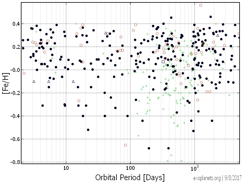
Figure 3: Plotting objects’ metallicity versus period shows that there exists an area that has a paucity of SLSS objects (filled black circles), but where the density of LSG objects (green crosses) is not lower than elsewhere. There are no SLSS objects with [Fe/H] greater than -0.03 in the range of periods from 653.22 to 923.8 days. The presence of six such objects in periods from 493.7 days to 923.8 days gives a much lower density than the adjacent areas. In contrast, of the 41 SLSS objects with lower [Fe/H] within the ROI, nine are within these period range. This area is also not empty of BS objects (red unfilled circles).

Figure 4: The distribution of objects by log period of the rSLSS objects (red, unfilled) compared with those of the other objects (green, filled). When wide bins the width of the full (shallow) gap are used, the gap region, with six objects with periods between 493.7 days to 923.8 days, still has a clearly lower density of objects per log period of rSLSS objects.

2.6 Patterns consistent between radial velocity searches

To consider whether the behavior of observers might have produced the features found here, a comparison of the results from different groups of astronomers might have produced different patterns. For example, if a group of observers conducted their RV search programs for only a limited number of years and then quit, then their data could have a maximum period, with a cutoff beyond they would not report any more systems. This apparent cutoff could show up in the data despite there being no such cutoff in the distribution of periods of real planets. This might account for the dropoff in periods beyond 493.7 days. It is a little more difficult to say that an observing group might have resumed its observations such that a sudden rise in the density of objects is produced. We studied the results from different observers whom we divided into two groups, and found that a peak-gap-peak pattern appeared separately in both sets of data. There may have been a different falloff of counts density at periods longer than 1000 days, as might be expected if there was more of a falloff in observing intensity of one group versus another. For different groups, blind to the presence of these features and blind to the other groups data, to produce data evidencing this peak-gap-peak pattern makes the chance that this pattern results from some behavior of the observing very unlikely.

An analysis of which radial velocity groups found how many objects in each of the peak, gap, and peak regions shows that the primary planet-finding groups maintained their observations for long enough to continuously find planets with periods longer than the long period pileup. There certainly was no mass stoppage of observing to produce a false dropoff in periods around 493.7 days, nor was there any mass restart of observing that could have caused the long period pileup.

Counting the numbers of which observing group discovered planets in the period ranges from inner peak through the gap and into the outer peak show no changes in the consistency of observers finding new planets. The fraction of planets found among rSLSS objects by each of the major groups that found planets remains similar from the short period peak to the long period peak.

The largest two groups finding planets started with the first discoveries of exoplanets. We combine counts of the planet discoveries of the smaller groups with the two largest groups and show the sums of planets found in period range in Table 2, where the “European” group was started in Switzerland by Mayor and Queloz,  (Mayor  Queloz, 1995), and is dominated by groups on the European continent except for the UK, which results from the “Anglo-Australian” collaboration we combine with the planets found by the “American” group started by Marcy and Butler,  (Butler  Marcy, 1996), along with results from a group from Japan and another U.S. group. Though there are only six rSLSS objects in the gap, these are also divided between the groups.

Both groups have found planets in all populations of periods well past 1000 days. We find that all of the main groups who found planets with periods in the first peak, up to 493.7 days, continued finding planets through the gap region, past the start of the deep gap at 923.8 days, and at least up to one gap width longer in log period, up to periods of 1729 days.

We also find that these same groups were finding SLBS objects and pSLSS objects, though there are fewer of these than rSLSS objects. We find that as far as can be detemined with the smaller number of these objects in the peaks, that the same groups continued to find planets throughout the period regions of the peak-gap-peak features. The SLBS and pSLSS populations do, however, have more objects in the gap region, and we see by the counts per group that these observers found objects in all these period regions at fractional rates similar to the fractions of total planets found by each group.

Table 2: Counts of planet discoveries by observing groups.

Regions	SP Peak	Gap	LP Peak
Start of period, days	263.8	493.7	$923.8$
End of period, days	493.7	923.8	$1728.6$
Counts total all groups
rSLSS	27	6	$32$
pSLSS	5	9	$9$
all SLBS	7	8	$9$
Counts by European and associated groups
rSLSS	11	4	$13$
pSLSS	2	6	$4$
all SLBS	4	3	$2$
Counts by U.S. and associated groups
rSLSS	15	2	$19$
pSLSS	2	3	$4$
all SLBS	3	2	$4$

3 Planet-mass limited “loner” selection has decreasing tail to peak ratio

Two more selections that further reduce the relative number of counts in the gap also enhance the peaks by producing a distribution of proportionately fewer objects in the tail regions away from the gap. We show that the ratios of the density of the tail counts divided by the density of the peak counts decrease for both the SPS and LPS. Using the densities in Table 1, in the rSLSS selection of 113 objects, the ratio of the densities of the tail regions to the gap-width “peak” regions on the SP (LP) side is 0.53 (0.48).

3.1 “Loner” and Jupiter-mass selections

When the rSLSS selection is divided into the 50 objects in multiple-planet and 63 objects in single planet systems (“multiples” and “loners”), the two distributions are strikingly different. Four of the six objects in the gap are among the multiples. The distribution of multiples is more uniform, having smaller or no peaks (Table 1).

In the selection of 63 loner rSLSS objects, there are two objects that remain in the gap, which is a slightly lower relative density. More significantly, both have $m$sin$i$ among the low and high extremes of the $m$sin$i$ distribution of rlSLSS objects. The features here are primarily features of the 56 objects of planet mass similar to Jupiter’s.

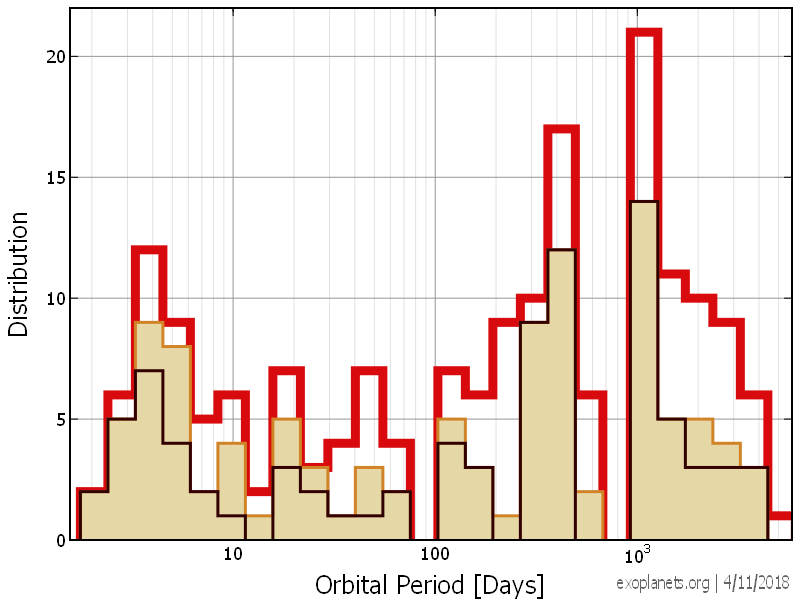
Figure 5: The two peaks become more distinct in the loner rSLSS selection (orange), and even more distinct when a cut to intermediate $m$sin$i$ (black) of 0.3 < $m$ sin $i$ < 9.0 $M_{J}$ is performed. The rSLSS counts are shown in red. Half-gap width bins are used since these selections have closer to half as many objects as in the rSLSS selection, which gives numbers per bin that are similar to Figures 1 and 2.

Finally, it is expected that planet distributions depend on planet mass, and indeed, the only two objects remaining in the gap region are in the low and high extremes of the $m$sin$i$ distribution. One is slightly under 0.3 $M_{J}$, which is one of the two objects lowest in $m$sin$i$, and the other is nearly 9.5 $M_{J}$, one of the five objects highest in $m$sin$i$. This makes it possible to take cuts of a minimum $m$sin$i$ of 0.30 $M_{J}$ and a maximum $m$sin$i$ of 9.0 $M_{J}$ leaving the 56 middle-mass “rich lone Jupiters,” or “rlJ” objects.The distribution of the 56 rlJ objects are are shown in orange in Figure 5.

Limiting our selection to these 56 rlJ objects with $m$sin$i$ in between the $m$sin$i$ of these two objects reveals that these “middle-mass” objects are even more concentrated in the two peaks compared to their tails (Figure 5 and Table 1).

3.2 Relatively more objects in the two peaks in “Loner” and Jupiter-mass selections

As we make the cuts going from the rSLSS to the loner selection, and then to the rlJ selection, each step removes more multiple objects from both tails than from the peaks. The result is that in the loner selection, the two peaks and gap become more distinct with each step. Using the ratio of the densities of the tail regions away from the gap to the peak regions near the gap shows how the two peaks on both sides of the gap become more dominant among the loner rSLSS and rlJ selections.

Although these further two cuts were performed blind to the rest of the distribution, they not only reduced the number of objects in the gap to zero, but reduced the number of objects away from the peak much more than in the peak. This can be quantified by how these cuts reduced the tail to peak density ratio.

We use values from Table 1 to calculate that the tail to peak density ratios for the SPS and LPS respectively go from 0.53 and 0.48 for the rSLSS selection to 0.28 and 0.37 for the loner rSLSS selection, and then to 0.22 and 0.28 for the rlJ selection.

The two peaks are the primary features for these middle-mass single-planet metal-rich single-star objects, suggesting that for this population of objects, planet formation most generously produces planets in the period bands of these two peaks.

3.2.1 Mean densities including of the stricter selections

The mean densities per gap width of the rSLSS selections, loner rSLSS, multiples rSLSS, and rlJ selections are the number of objects in each selection divided by 6.24 gap widths of the ROI.

So the mean densities are 18.01 objects for the 113 objects in the rSLSS selection, 10.1 for the 63 objects in the loner rSLSS selection, 8.0 for the 50 objects in the multiples rSLSS selection, and 9.0 for the 56 objects in the rlJ selection.

Going from the rSLSS selection to the loner rSLSS selection reduces the relative density from 0.33 +- 0.14 to 0.20 +-0.14 of the mean densities, while the relative density of the rmSLSS selection increases to 0.50 +- 0.25.

4 Other populations have only one single pileup in region of the double-peaked pileup

The sum of the other selections shows that the same region is part of the peak of the other populations (Figure 1, green filled-in bins). There is no dip in the LSG selection or in the pSLSS selection below [Fe/H] of -0.07. This region is also high in counts in the SLBS selection, though the counts are too low to consider smaller regions such as the deep part. We look at counts in the gap region of the combined grouping of the 198 “Other” objects in the three other selections: the LSG, SLBS, and pSLSS selections.

We show the metallicity distribution by period of all objects in Figure 3. The black filled circles for the SLSS selection show that there is a gap region for metallicities above a boundary that actually is closer to [Fe/H] of -0.03, though for simplicity we have used [Fe/H] of zero in most of the presentation here. The planets in “other” selections are those hosted by stars of low surface gravity (LSG, green crosses), stars that are sunlike (in surface gravity) but have at least a binary stellar companion (SLBS, red unfilled circles), or are sunlike single stars poorer in metallicity than the sun (pSLSS). (Squares denote two SLSS objects outside of “sunlike” effective temperatures, of 4500 < $T_{eff}$ < 6500 K.)

There are 63 “other” objects in the region of the gap in rSLSS objects, where we sum values from the pSLSS, BS, and LSG populations (as shown in Table 1). Of these three other selections, when considered separately only the BS selection has a possible sign of a gap. So the rSLSS gap region is part of the peak in density for other regions, as there are nearly twice as many “other” objects as the ROI mean density, but only one third the mean density of rSLSS objects.

We will also use the “deep part” of the gap where there are zero rSLSS objects to demonstrate how unlikely it is for there to be a region where there are no rSLSS objects, because it is especially straightforward to calculate the unlikelihood of having a region of objects every one of which is outside the rSLSS selection. This deep part is the longward 0.55 fraction of the gap or 0.089 of the ROI, consisting of the region from the periods of 653.2 to 923.8 days. If a region this wide were populated at the mean density, it would have 0.089 of the objects, or 17.5 “other” and 10.0 rSLSS objects, but there are 33 “other” objects and 0 rSLSS objects. Since the deep part has close to twice (1.9) the mean number of “other” objects as the mean, it is again part of the peak of the other three selections.

The presence of so many objects in the other populations where there are few or none in the rSLSS population is evidence against the gap being an observational effect: there could not be an observational failure to find rSLSS objects but not other objects in just one period range. Though these data might be subject to selection effects due to having been collected by many different observers, it is extremely unlikely for any observational effect to reduce only the rSLSS population but not the other populations.

5 Unlikelihood demonstrated from more than one perspective

We show that a gap this wide that divides the peak of the pileup into two peaks is unlikely to be produced at random from two perspectives:
(1) Considering only the distribution of rSLSS objects alone, and
(2) comparing the distribution of rSLSS objects alone with the distribution of the other selections.

In each case, we can calculate the likelihood of the existence of only the more narrow region with zero objects (the “deep gap”), or the wider full region between the peaks that has a lower density but still has a small number of objects. We also calculate how likely it is for both to exist. We are careful in our calculations to count allowing the positioning of these gaps to occur anywhere within a region containing at least the inner part of two peaks, to not artificially require that the random features match the specific positioning of the gaps that we find.

This wide of a gap separating the peak of the pileup into two peaks is unlikely to be produced at random by first considering the likelihood of a gap in distribution, and second, considering the likelihood of a consecutive string of values to entirely come from a subset of our full dataset.

The gap between the peaks is unlikely to be random from two perspectives: It is unlikely that the rSLSS population has the shallow and deep gaps, and it is unlikely that there is a wide region with no gap in the populations outside of the rSLSS population such that all of the 33 objects in the region of the deep gap come from the other 60$\%$ of the total population.

We discuss two important ways of looking at the peaks and the gap:
1. Emphasizing the separation between two peaks that has a low density (six objects), or
2. Emphasizing the gap as a region where the distribution of planets has so few objects that from the current data there are zero objects.

To model how the gap has the two subregions, one of low density and one of zero objects, we consider two models based on two simplications of the gap: (1) The wide low density region encompassing the full shallow gap, and (2) the narrow but deeper region encompassing the deep gap. The deep gap encompasses a little more than half of the long period part of the shallow gap. Note that the sharpest transition is the boundary going from the long period edge of both gaps to the longer period peak, marked by the object having a period of 923.8 days.

We first consider only the objects in the rSLSS population as distributed by log period, and show that the log period distribution gap is unlikely, especially in between two peaks.

We follow by considering how there are 33 objects in the main other selections in the period range of the deep gap where there are zero objects in the rSLSS selections. Since the rSLSS selection contains nearly 40$\%$ of the total objects, this means that the number of rSLSS objects in the range should be closer to 22 objects. It can be seen in the histogram of the total counts, Figure 1, that there is in fact a dip in the total counts in the range of the deep gap. We cite the presence of this dip to argue that the deep gap of rSLSS objects cannot be due to incorrect measurements of surface gravity leading to misclassification of objects in this period range.

5.1 Likelihoods of a “gap” or region of low density

We list in Table 3 the likelihoods calculated how often random distributions produced gaps by taking two views of the gap, and then considering them together:

1. The more narrow “deep part” of the gap that contains zero objects, of periods from 653.22 to 923.8 d.

2. The wider full gap that contains six objects, with periods from 493.7 up to 923.8 days.

The true likelihood would be somewhere in between choosing a range near the peaks of the distribution, where the gaps occur, and in choosing most of the ROI from 100 to 5000 day periods. Choosing most of the ROI underestimates the likelihood by allowing the gap to appear in a lower density of counts per log period than the gap actually occurs in, as well by allowing a gap to occur either on the short or long period end where the gap would merely cause a shorter or longer pileup rather than splitting the gap in two. Choosing a gap in too narrow of a range falsely reduces the range in which it may occur. We choose two reasonable ranges and suggest that the true likelihood is in between the two calculated likelihoods.

5.1.1 Deep part of gap with zero objects unlikely in random distribution

Because all six of the rSLSS objects in the gap are in the short period side in less than half of the shallow gap, the longer part of the gap with zero rSLSS objects, which we call the “deep part” of the gap. These six have periods above the ending of the SPP at the period of 493.7 days, to the longest at 653.22 days. The deep gap with zero objects thus goes from the period of 653.22 to the starting period of the LPP at 923.8 days, which covers a distance of 0.150 in log period space, or 0.089 of the ROI, and which is 0.55 of the width of the shallow gap. If a region with 0.089 of the ROI had the mean density of rSLSS objects in the entire ROI including the tails, it would have 10.0 objects. Both the full gap and the deep part represent a significant deficit relative to even a uniform distribution, but this gap structure is most significant relative to how the two pileups that are on both sides have their highest densities of counts per log period next to the gaps. More than half of the objects in both peaks are within one shallow gap width of 0.272 in log period of the shallow gap. Of the 49 objects on the short period side of the gap, 27 are within this 0.16 of the ROI, and of the 58 objects on the long period gap, 32 are within this distance that has only six objects in the gap. This means that if the shallow gap had the same density as the mean density of the same width on each side, it should have closer to 29.5 rSLSS objects, not just six.

We show in Section 5.1.2 that the likelihood of these features occurring at random starts at only 1 in 5000 when only parts of these features are considered, such as having the deep gap in a uniform distribution, but the likelihood becomes even less when considering more aspects of the distribution.

5.1.2 Likelihood of gap randomly appearing in observations if the physical distribution has no gap

To see how likely this gap would appear at random, we conducted Monte Carlo simulations of either uniform or peaked distributions to see how often an equivalently significant gap appears anywhere within selected regions of interest (ROIs) encompassing the peak. Though the likelihood varies depending on how wide of an ROI is chosen, we find that the gap in the rSLSS population is extremely unlikely to be a random feature, at the level of less than one in $10^{4}$ random instances.

If modeling that the likelihood of a random gap appearing in a distribution that is actually physically characterized by a single pileup, this gap would occur somewhere near the center of the pileup. This means that we do not allow the gap to occur too close to either the short period or long period edge. This means that we calculate the chance that this gap will occur only in a selected smaller region, and thus count only the number of objects within this selected region. It is a matter of judgment to consider how large of a subregion to choose, but we choose subregions that are still large relative to the full pileup. Rather than trying to argue for on size of a subregion, we perform two calculations of unlikelihood is performed within the following two ranges that we argue bracket the true unlikelihood with one value too high and one too low.

1.) A range of one in log period, and

2.) a “three-gap-width” range going from one shallow gap width of 0.272 below to one width above the shallow gap, for a range of 0.816 in log period (three times 0.272).

The first subregion is wide, allowing the gap to be far from the center such that the true unlikelihood is probably higher than the calculated value for this region. The 2nd is small, where it might be argued that the 2nd small region presupposes the existence of the gap:

We summarize the evaluation by Monte Carlo of several cases in Table 3. For assessing the likelihood of an equivalent gap appearing at random when supposing the actual underlying population has no gap, we have developed a Monte Carlo program to test likelihood of an equivalent gap occurring with the same number of data points, $N_{range}$. We computed what the width of an equivalent gap would be for a range from 0 to 1 first by considering the fraction that the gap width is of the width of the outer pileup, and then second calculating what fraction of the period region that contains the peak of the pileup does this gap represent. We are then able to use how often a random distribution of $N_{range}$ values in between zero and one have a gap as large as this fraction to evaluate how likely it is to have a gap occur near the middle of the peak of the pileup. The Monte Carlo program obtains the likelihood of the gap by,

1.) Creating vectors of $N_{range}$ random values in between 0 and 1,

2.) Taking the difference in between each point, and then finding the largest difference.

3.) Seeing what fraction of random vectors has a difference as large as the gap.

We compare what likelihood is obtained this way, when we use the density of the peaks outside the gap while using the counts per log period from the one-log-period range from 200 to 2000, and 300 to 3000 day periods, and find it makes little difference. From 200 to 2000 day periods, there are $N_{range}$ = 79 objects. While this is a density of 79 objects per log period for this selected period range, there is a higher density for the part of the range outside the gap, which has a length of 1.0-0.272=0.728 log period and has 73 objects after subtracting the six in the gap. The density for just that part is 73/0.728, or a much higher value of 100.3 objects per log period. From 300 to 3000 day periods, there are 78 objects in our selection. Here there are 72 objects in just the region outside the gap. Outside the gap, there is a density of 98.9 objects per log period for the range 200 to 2000 days. So using either range we obtain a density in the peaks of close to 100 objects per log period.

We find that even in the case of allowing a gap of zero objects with a width of 0.089 in log period to appear anywhere in a distribution of the 79 objects randomly placed in the range of 1 in log period, from 300 to 3000 days, that the frequency of the deep part of the gap randomly appearing is less than one in 5000 random instances. The occurrence of the full (shallow) gap with six objects in a region of 0.1505 is a little more than 1 in 2000 instances. For a region with as low density as the deep part of the gap to occur anywhere within a wider shallow gap of these widths happens only once in in $4\times 10^{4}$ times.

However, because a range of one in log period includes some of the tails as well as the peaks, this underestimates the likelihood because by allowing the gap to fall anywhere, it could fall to the sides, in which case the gap would not really be creating two peaks. We seek to bracket the actual likelihood by also considering a more narrow range. Since this may overestimate how unlikely this feature is, we believe that the true likelihood is somewhere in between the likelihoods found using these two ranges. We now consider the likelihood that the gap occurs near the peak of the pileup, so that we require that the gap occur in slightly less wide regions bounded by the peaks. We find using Table 1 that there are 65 objects which are bounded within one full gap width of the gap, with periods from 263 to 1729 days, which is a log period distance of 0.816. The 65 objects include the six in the gap, and 59 in the peaks which comprise most of the high density regions. We then evaluate the likelihood of the gaps occurring among 65 objects. The shallow gap fills one third of this “three-gap-width” range, and the deep part of the gap which is 0.55 of the gap width, fills 0.18 of this range. The number of times that the shallow gap and deep part occur only once in numbers that approach or exceed one in $10^{5}$ instances, depending on how fully we match the peak of the pileup to the double peaks.

These results show that these gaps are extremely unlikely to be due to random.

The calculations considering the likelihood of a deep gap within the full gap do not quite account for how other configurations of inner and outer gaps would also be called unlikely. We could consider that the shallow part might have more objects but that the deep gap is wider, or that the shallow part would have fewer objects but the deep gap is more narrow. These alternatives must be added into a two-level evaluation, but it is hard to assign the width of the deep gap in such cases. We could say that the actual likelihood of any surprising gap is perhaps two or three times greater than the one we consider here, but we suggest that even if we did perform this two-level evaluation, we are still talking about such a very unlikely random gap that at this point, the main point is that this gap is extremely unlikely to appear at random.

Table 3: Summary of likelihoods bracketed between calculations using wide and narrow ranges that the gap might appear Numbers of objects, fractional span of the gap, and likelihoods. Above: Fraction of random distributions that show a gap as large as the deep gap, the shallow gap, or both together. Below: The inverse fraction, or “one in how many” random distributions does the gap occur.

Range	Number of objects	Deep-Part		Full Gap		Both-Together
Log-one in period	79	0.151	$2.0e-4$	0.272	5.5 e-4	2.5 e-5
Three $\times$ Shallow Gap	65	0.184	$1.1e-4$	0.333	2.2 e-4	1.2 e-5
One-out-of:
Range		Deep-Gap		Full Gap		Both-Together
Log-one in period	79		$5263$		1852	40000
Three $\times$ Shallow Gap	65		$9091$		4545	85000

5.2 “Other” three selections have single pileup with no gap

We compare how many objects in each group are in the region with how many objects in each group would be expected to be in a region this wide if the distribution were uniform in the ROI.

We consider whether the sum of all “other” objects has any gap. The “other” selection consists of 198 objects, summed from the 123 LSG, 34 SLBS, and 41 pSLSS objects in the ROI (Table 1). The mean density of the gap-width region that is 0.27 in log period, which is 0.160 of the 1.70 log period width of the ROI, is then 31.7 objects (of all types) per gap-width.

The shallow gap has only six rSLSS objects, compared to a mean of 18.1 rSLSS objects per 0.27 log period, yet the same period region from 493.7 to 923.8 days contains 63 “others” compared to a mean density of 31.7 other objects per gap-width bin of 0.160 of the ROI. These 63 “others” break down into the other three populations, followed by the mean number of objects in a bin this size, as follows:

46 LSG objects versus a mean of 19.7 LSG objects;

8 SLBS objects versus a mean of 5.5 SLBS objects; and

9 pSLSS objects versus mean of 6.6 pSLSS objects.

(If we subdivide the SLBS selection in order to compare metal-rich objects that have stellar companions with our rSLSS selection hosted by single stars, the 8 SLBS objects are composed of 3 pSLBS versus a mean of 1.2 pSLBS objects per bin, and 5 rSLBS versus a mean of 4.3 objects per bin. So, though the numbers are too low to give strong statistics, it appears probable that neither the metal-rich or metal-poor selections of the SLBS selection shows a sign of a gap.)

All three of the “other” populations have a higher count in this period range, meaning the region of the shallow gap in the rSLSS population corresponds to a region that in all three other populations is part of the peaks of those populations.

When we narrow our evaluation to the deep part of the gap where there are zero rSLSS objects, the 0.151 log period between periods of 653.2 to 923.8 days, or 0.089 of the ROI, compared to a mean of 10.01 “other” objects there are 33 “other” objects in this region. This compares to a mean density of 17.5 “other” objects in a mean width of 0.089 of the ROI. These 33 others similarly break down as follows:

25 LSG objects versus a mean of 10.9 LSG objects;

2 SLBS objects versus a mean of 3.0 SLBS objects; and

6 pSLSS objects versus a mean of 3.6 pSLSS objects.

The LSG and pSLSS population densities are still high in the region of the deep gap. The the two SLBS objects are a statistically insignificant one count below the mean of three such objects in this region. (Both are rSLBS objects.) Whether this represents a partial gap among the SLBS population requires more data.

The distributions of the other 198 objects in the three populations in the ROI do not have any such deep gaps. The 123 LSG objects in the ROI are enough to say this selection has no sign of any gaps. Though the number of objects are not high enough among the 41 pSLSS and 34 SLBS objects to be strongly significant, it appears that there is no region with similarly few objects in the distribution of periods of the LSG population.

The counts of LSG and pSLSS objects are still high compared to their means in this region; the count of two objects in the rSLBS selection in the region of the deep gap could be low, but is not zero. This shows that there is no sign of a gap in the LSG distribution.

There is also no sign of a gap in the pSLSS population, though we see from Figure 3 that this best applies to moving the boundary of “metal poor” to be at an [Fe/H] of below -0.07. The deep part of the gap region in the rSLSS population is part of the peak of pSLSS objects, especially if the boundary is taken lower to be at an [Fe/H] of -0.07.

For the 34 objects where the star has a stellar companion, the ROI contains 27 rSLBS objects and seven pSLBS For the deep part of the gap region to contain two out of all 27 rSLBS objects in the ROI, compared to zero of 113 rSLSS objects in this same period region, this could be an indication that the presence of a stellar companion could cause planet periods to evolve to partially fill in the gap. The two counts still produce a lower density of rSLBS objects in the gap region, which density is much lower than the neighboring regions that correspond to the peaks. Due to the statistically small numbers of these rSLBS objects, however, the most that can be concluded is that the rSLBS population could have a partial gap in the region of the deep part of the rSLSS gap.

5.2.1 Gap unlikely to randomly appear in observations of only one selection

It is unlikely that the deep gap would occur in the rSLSS selection of 113 of the 313 total objects with periods past 100 days, which is 36% of the exoplanet population in the main region, but not occur in the distribution of the remaining 200 objects, or 60% of the objects in the database. In the region of periods from 653.2 to 923.8 days where there are zero rSLSS objects, this means that the 33 other objects appear in a consecutive series of not having any rSLSS objects. For each of the 33 objects, there should be a 36% chance of the object being an rSLSS object. So the chance of having 33 consecutive objects that are not rSLSS objects is the value calculated by,

280(1 - 113/313)³³=1.1 $\times$ 10^-4,

which is less than one random distribution in 9000.

This shows that it would be extremely difficult for an observational effect to create such a gap. The fact that this “excluded selection,” composed of LSG, metal-poor and binary star objects, has so many objects with the same period region that the rSLSS selection has a gap argues against that an observational effect to be responsible. Such an observational effect would have to make objects of stars that are sunlike partially undetected and partially misclassified, while simultaneously not affecting detections of objects that are too low in temperature, too high in surface gravity, or are too low in metallicity, as well as only partially affecting planets of stars that have a binary companion. If such an observational effect exists, it is important to understand it. We submit that such an effect is extremely unlikely, leaving the explanation that the gap is a physical feature.

Figure 6: Counts of objects that are not hosted by above solar metallicity sunlike stars, in thick green lines, compared to the total of all objects found by RV (light filled tan lines), metal-rich sunlike objects (red unfilled lines) and metal-poor sunlike objects (blue filled lines).

6 Discussion: What might cause the gaps and peaks?

The presence of these observational features challenges the current paradigm which maintains that planet formation is stochastic and cannot be regular. It is especially difficult to reconcile such a sharp feature as the sudden rise in the number of objects which occurs at periods above 920 days. It is difficult for a snowline trap to play such a role, since the snowline changes during evolution of the solar nebula. If the snowline does play a role, then it might require that there be a special time in this evolution that would trap planets at periods above 920 days. It is even more difficult to suggest that planets either do not migrate from higher periods than 920 days down to lower periods, or that all planets that form at periods less than 920 days are migrated to periods longer than 920 days.

We also consider the model of Christodoulou  Kazanas (2019)(hereafter CK19) who suggest that nebular material is trapped by density oscillations driven by the density of the material being described by the Lane-Emden equation oscillating around boundary conditions that the equation cannot satisfy. The two peaks could be the two lowest period regions of such high density regions. However, the CK19 hypothesis supposes a much higher degree of regularity of multiplanet systems than is generally accepted. The test of the CK19 hypothesis is to test it further on more multi-planet systems.

The regular features found here stand in contrast to the lack of regular features at longer periods of protoplanetary disks observed by the DSHARP project conducted by the ALMA observatory (Andrews ., 2018; Huang ., 2018). The resolution of ALMA is not high enough to resolve structures closer in than 10 AU, and of course the DSHARP results are observations of disk material rather than planets, so the results here do not disagree with the DSHARP results. Still, this discrepancy implies that the inner later positioning of planets is more regular than the outer earlier positioning of nebular material. We encourage efforts to image protoplanetary disks at higher resolution.

These results show the importance of continuing to find more giant planets at periods of hundreds to thousands of days which have measurable parameters. The current data set is dominated by stars of mass not too different from solar mass, so it would help to find more planets of lower mass stars to better see how these features depend on stellar mass.

Planets found using the RV method are ideal in that the system parameters are generally well measured.

It is expected that WFIRST (Spergel ., 2015) will find many planets within this region, but to evaluate these patterns it is important that the planet-hosting stars be recovered and more system parameters than just the planet and star masses be measured. It is most important to measure the period, stellar surface gravity, and the metallicity. Even without measuring the stellar surface gravity and metallicity, when the bulk planet set is plotted by period there exists an identifiable notch in the location of the gaps. So even if only the period is found, the WFIRST results may contribute to understanding these features.

7 Summary

The log period distribution of these objects has a bimodal pileup as opposed to the single pileup of iron-poor objects. In contrast, the distribution of periods of LSG and pSLSS objects beyond 100 days have single pileups. Though the number of BS objects is small, this group has a few objects within the gap, so it is not clear whether the periods of BS objects have a partial double peak distribution or have a single pileup.

We show that looking at the distribution of periods of the rSLSS selection alone it is unlikely that a gap this wide would randomly show up in 113 objects. We also consider how unlikely it is within this range corresponding to 33 objects that there is a string of 33 objects all outside the rSLSS selection. This is not only unlikely to occur at random, but it is also unlikely that observational effects would somehow not find the objects in the rSLSS selection without decreasing the counts outside the rSLSS selection. We also address the possibility of observational effects by comparing the distributions found by different groups of observers. Other than possible dropoffs at longer periods due to reduced observations, the planets found by different groups follow the same general patterns of a valley up to perhaps 200 days with a pileup at longer periods. We see that the distributions from different observer groups similarly show this gap-peak-gap feature, demonstrating that it is unlikely that the manner in which observations were taken falsely generated this pattern.

Features of the peaks that indicate underlying structure include that the long period gap is most dense near the boundary with the gap taken to be the period of 923.8 days. Though the gap is found in both single and multiple planet systems, the two peaks are relatively even more prominent when only single-planet systems are considered. The only remaining two objects in the gap have one with a low mass and one with a high mass, suggesting that the full gap is a feature of planets with mass not too much more or less than Jupiter’s.

In contrast, there is only a single peak of LSG and pSLSS objects. Among the rSLBS population, though there are objects within the gap, there could be two separate peaks in the rSLBS selection. More SLBS objects are needed to see the shape of the distribution of SLBS objects.

We find that the peak-gap-peak pattern is unlikely to occur either as random or as a result of observations. To see how likely these gaps are in just the rSLSS distribution, we tested random distributions of the peak parts of the distribution, consisting of more than half of the 113 objects within the periods of 100 to 5000 days, which is a log period span of 1.7. We found that even in a log period span of 1.0, that it is unlikely to have a log period distance of 0.15 of the distribution not have any objects at the level of one in many thousands. It is similarly unlikely that a log period distance of 0.272 will have only six objects. When considering all the populations of objects, we find it unlikely that there will be a consecutive string of 33 objects without any rSLSS objects.

8 Conclusions

That these patterns show up in the aggregate of so many different systems is evidence that planet formation and evolution must have much more uniformity than previously assumed. Perhaps the biggest surprise, as gauged by the responses to when these results have been presented, is that planet evolution is thought to be too chaotic to preserve such distinct features. While it is not surprising that there is an increase in counts corresponding to an important condensation temperature, the presence of such a deep gap at periods shortward of the main peak, with another shorter period pileup, represents a new major unexpected feature of the distribution of a very large fraction of exoplanetary systems. How these features form, and how they remain preserved in the cumulative distribution, are now important questions that must be answered if we are to understand planet formation.

References

- Andrews \BOthers. (\APACyear2018) \APACinsertmetastarand18{APACrefauthors}Andrews, S\BPBIM., Huang, J., Pérez, L\BPBIM. et al. \APACrefYearMonthDay2018Dec, \APACjournalVolNumPagesApJ8692L41. \PrintBackRefs\CurrentBib
- Butler \BBA Marcy (\APACyear1996) \APACinsertmetastarmar96{APACrefauthors}Butler, R\BPBIP.\BCBT \BBA Marcy, G\BPBIW. \APACrefYearMonthDay1996\APACmonth06, \APACjournalVolNumPagesApJ464L153. \PrintBackRefs\CurrentBib
- Christodoulou \BBA Kazanas (\APACyear2019) \APACinsertmetastarchr19{APACrefauthors}Christodoulou, D\BPBIM.\BCBT \BBA Kazanas, D. \APACrefYearMonthDay2019Jan, \APACjournalVolNumPagesarXiv e-prints. \PrintBackRefs\CurrentBib
- Dawson \BBA Murray-Clay (\APACyear2013) \APACinsertmetastardaw13{APACrefauthors}Dawson, R\BPBII.\BCBT \BBA Murray-Clay, R\BPBIA. \APACrefYearMonthDay2013\APACmonth04, \APACjournalVolNumPagesApJ767L24. \PrintBackRefs\CurrentBib
- Fischer \BBA Valenti (\APACyear2005) \APACinsertmetastarFis05{APACrefauthors}Fischer, D\BPBIA.\BCBT \BBA Valenti, J. \APACrefYearMonthDay2005\APACmonth04, \APACjournalVolNumPagesApJ6221102-1117. \PrintBackRefs\CurrentBib
- Gonzalez (\APACyear1997) \APACinsertmetastargon97{APACrefauthors}Gonzalez, G. \APACrefYearMonthDay1997\APACmonth02, \APACjournalVolNumPagesMNRAS285403-412. \PrintBackRefs\CurrentBib
- Han \BOthers. (\APACyear2014) \APACinsertmetastarhan14{APACrefauthors}Han, E., Wang, S\BPBIX., Wright, J\BPBIT. et al. \APACrefYearMonthDay2014\APACmonth09, \APACjournalVolNumPagesPASP126827. \PrintBackRefs\CurrentBib
- Huang \BOthers. (\APACyear2018) \APACinsertmetastarhua18{APACrefauthors}Huang, J., Andrews, S\BPBIM., Dullemond, C\BPBIP. et al. \APACrefYearMonthDay2018Dec, \APACjournalVolNumPagesApJ8692L42. \PrintBackRefs\CurrentBib
- Mayor \BBA Queloz (\APACyear1995) \APACinsertmetastarmay95{APACrefauthors}Mayor, M.\BCBT \BBA Queloz, D. \APACrefYearMonthDay1995\APACmonth11, \APACjournalVolNumPagesNature378355-359. \PrintBackRefs\CurrentBib
- Santos \BOthers. (\APACyear2003) \APACinsertmetastarsant03{APACrefauthors}Santos, N\BPBIC., Israelian, G., Mayor, M., Rebolo, R.\BCBL \BBA Udry, S. \APACrefYearMonthDay2003\APACmonth01, \APACjournalVolNumPagesA&A398363-376. \PrintBackRefs\CurrentBib
- Spergel \BOthers. (\APACyear2015) \APACinsertmetastarspe15{APACrefauthors}Spergel, D., Gehrels, N., Baltay, C. et al. \APACrefYearMonthDay2015Mar, \APACjournalVolNumPagesarXiv e-printsarXiv:1503.03757. \PrintBackRefs\CurrentBib
- Taylor (\APACyear2012) \APACinsertmetastartay12b{APACrefauthors}Taylor, S\BPBIF. \APACrefYearMonthDay2012\APACmonth11, \APACjournalVolNumPagesArXiv e-prints. \PrintBackRefs\CurrentBib
- Taylor (\APACyear2013) \APACinsertmetastartay13b{APACrefauthors}Taylor, S\BPBIF. \APACrefYearMonthDay2013\APACmonth05, \APACjournalVolNumPagesArXiv e-prints. \PrintBackRefs\CurrentBib
- Udry \BBA Santos (\APACyear2007) \APACinsertmetastarudr03{APACrefauthors}Udry, S.\BCBT \BBA Santos, N\BPBIC. \APACrefYearMonthDay2007\APACmonth09, \APACjournalVolNumPagesARA&A45397-439. \PrintBackRefs\CurrentBib