Bounding Radon number via Betti numbers

Abstract.

We prove general topological Radon-type theorems for sets in $\mathbb{R}^{d}$ or on a surface. Combined with a recent result of Holmsen and Lee, we also obtain fractional Helly theorem, and consequently the existence of weak $\varepsilon$-nets as well as a $(p,q)$-theorem for those sets.

More precisely, given a family $\mathcal{F}$ of subsets of $\mathbb{R}^{d}$, we will measure the homological complexity of $\mathcal{F}$ by the supremum of the first $\lceil d/2\rceil$ reduced Betti numbers of $\bigcap\mathcal{G}$ over all $\mathcal{G}\subsetneq\mathcal{F}$. We show that if $\mathcal{F}$ has homological complexity at most $b$, the Radon number of $\mathcal{F}$ is bounded in terms of $b$ and $d$. In case that $\mathcal{F}$ lives on a surface and the number of connected components of $\bigcap\mathcal{G}$ over all $\mathcal{G}\subsetneq\mathcal{F}$ is at most $b$, then the Radon number of $\mathcal{F}$ is bounded by a function depending only on $b$ and the surface itself.

Concerning fractional Helly theorem, we get the following improvement using the recent result of the author and Kalai: Let $\mathcal{F}$ be a family of open sets in a surface $S$ such that for every $\mathcal{G}\subsetneq\mathcal{F}$, $\bigcap\mathcal{G}$ has at most $b$ path-connected components. Then the fractional Helly number of $\mathcal{F}$ is linear in $b$. Specifically, for $b=1$ we show that the fractional Helly number is at most three, which is optimal. This case further leads to solving a conjecture of Holmsen, Kim, and Lee about an existence of a $(p,q)$-theorem for open subsets of a surface.

1. Introduction

Radon’s theorem [Rad21] is a central result in convex geometry. It states that it is possible to split any $d+2$ points in $\mathbb{R}^{d}$ into two disjoint parts whose convex hulls intersect. It is natural to ask what happens to the statement, if one replaces convexity with a more general notion.

Perhaps the most versatile generalization of the convex hull is the following. Let $X$ be an underlying set and let $\mathcal{F}$ be a family of subsets of $X$. Let $S\subseteq X$ be a set. The $\mathcal{F}$-hull $\operatorname{conv}_{\mathcal{F}}(S)$ of $S$ relative to $\mathcal{F}$ is defined as the intersection of all sets from $\mathcal{F}$ that contain $S$. If there is no such set, the $\mathcal{F}$-hull is, by definition, $X$. This definition is closely related to so called convexity spaces, which we discuss in Appendix A. Note that if $\mathcal{F}$ is a family of all convex sets in $\mathbb{R}^{d}$, then $\operatorname{conv}_{\mathcal{F}}$ coincides with the standard convex hull.

The Radon number $r(\mathcal{F})$ of $\mathcal{F}$ is the smallest integer $r$ such that any set $S\subseteq X$ of cardinality $r$ can be split into two disjoint parts $S=P_{1}\sqcup P_{2}$ satisfying $\operatorname{conv}_{\mathcal{F}}(P_{1})\cap\operatorname{conv}_{\mathcal{F}}(P_{2})\neq\emptyset$. If no such $r$ exists, we put $r(\mathcal{F})=\infty$.

Radon numbers and their relatives are studied not only in convex or discrete geometry [Eck93, Tve66, BB79, Eck76, KK76, etc.], but they found applications also in computational geometry [CEM⁺96], computational complexity [Onn91, MS10], optimization [Bro65, Ame94], robust statistics [ABET00], operation research [QT17], or parallel machine learning [KBMG17].

In this paper we show that very mild topological conditions are enough to force a bound on Radon number for sets in Euclidean space (Theorem 2.1) or on surfaces (Theorem 2.2). A simple trick allows us to give a version of the result for smooth manifolds or simplicial complexes, see Section 2.1. In Section 2.2 we list some important consequences, most notably fractional Helly theorems (Theorems 2.3 and 2.4), which, with some further tools (Theorem 2.5) lead to solving a conjecture of Holmsen, Kim, and Lee [HKL19, Conj. 5.3] (a special case of Theorem 2.6). In the appendix we disccuss a relation between convexity spaces and our setting.

2. Results

Radon’s theorem [Rad21] provides an upper bound on the Radon number of convex sets. However, this property is preserved by an arbitrary topological deformation of $\mathbb{R}^{d}$. Bounded Radon number is thus not a property that holds merely for standard convex sets. In this paper we prove that the Radon number $r(\mathcal{F})$ of a family $\mathcal{F}$ is bounded whenever $\mathcal{F}$ is “not too topologically complicated”. Let us first explain what “not too topologically complicated” means.

Homological complexity. Let $k\geq 1$ be an integer or $\infty$ and $\mathcal{F}$ a family of sets in a topological space $\mathbf{R}$. We use the notation $\bigcap\mathcal{F}:=\bigcap_{F\in\mathcal{F}}F$ as a shorthand for the intersection of a family of sets. We consider singular homology with coefficients in $\mathbb{Z}_{2}$ and denote by $\tilde{\beta}_{i}(X;\mathbb{Z}_{2})$ the $i$th reduced Betti number of $X\subseteq\mathbf{R}$. We define the $k$-level homological complexity of $\mathcal{F}$ as:

$$\sup\left\{\widetilde{\beta}_{i}\left(\bigcap\mathcal{G};\mathbb{Z}_{2}\right)\colon\mathcal{G}\subsetneq\mathcal{F},0\leq i<k\right\}$$

and denote it by $HC_{k}(\mathcal{F})$. We call the number $HC_{\infty}(\mathcal{F})$ the (full) homological complexity. The definition makes sense also for other rings of coefficients. Note that even if the family $\mathcal{F}$ lives in $\mathbb{R}^{d}$, it may happen that $\tilde{\beta}_{k}(\bigcap\mathcal{G};\mathbb{Q})>0$ for $k>d$ and some $\mathcal{G}\subsetneq\mathcal{F}$, see [BM62], albeit we do not know whether this can also happen for $\mathbb{Z}_{2}$-coefficients. In any case, for the reasons explained in Section 5, we use the homology with $\mathbb{Z}_{2}$-coefficients throughout the paper.

Many families we are used to work with have bounded homological complexity. To name a few: family of convex sets in $\mathbb{R}^{d}$, families of open sets in a topological space, where the intersection of each subfamily is either empty or homologically trivial (such families are called good covers), families of spheres and pseudospheres in $\mathbb{R}^{d}$, families of algebraic sets in $\mathbb{R}^{d}$ defined by polynomials of degree at most $D$ (By Milnor [Mil64], the Betti numbers of any algebraic set in $\mathbb{R}^{d}$ can be upper bounded by a function depending only on $d$ and $D$. Specifically, it doesn’t depend on the number of polynomials defining the variety.). Another example can be obtained as follows. We consider a family of polytopes in $\mathbb{R}^{d}$ whose all normals lie in some fixed finite set $S$, together with their polyhedral subcomplexes. It was shown in [GPP⁺17, Corollary 5] that homological complexity of such a family is bounded by a function of $|S|$ and $d$. As a special case we get a family of axis-alligned (hollow) boxes.

We can now state our main theorem.

Theorem 2.1 (Bounded mid-level homological complexity implies Radon).

For every non-negative integers $b$ and $d$ there is a number $r(b,d)$ such that the following holds: If $\mathcal{F}$ is a family of sets in $\mathbb{R}^{d}$ with $HC_{\lceil d/2\rceil}(\mathcal{F})\leq b$, then $r(\mathcal{F})\leq r(b,d)$.

We note that the bound $r(b,d)$ that our proof provides is very large (but still elementary recursive) as it relies on successive applications of Ramsey’s theorem. On the other hand, the bound on $r(\mathcal{F})$ is qualitatively sharp in the sense that all $\widetilde{\beta}_{i}$, $0\leq i<\lceil\frac{d}{2}\rceil$, need to be bounded in order to have a bounded Radon number. We discuss this in Section 5, Example 1.

2.1. Embeddability

We have seen that for a family of sets in $\mathbb{R}^{d}$, in order to have a bounded Radon number, it suffices to restrict the reduced Betti numbers up to $\lceil d/2\rceil-1$. Which Betti numbers do we need to restrict, if we replace $\mathbb{R}^{d}$ by some other topological space $\mathbf{R}$? The following paragraphs provide some simple bounds if $\mathbf{R}$ is a simplicial complex or a smooth real manifold. The base for the statements is the following simple observation: Given a topological space $\mathbf{R}$ embeddable into $\mathbb{R}^{d}$, we may view any subset of $\mathbf{R}$ as a subset of $\mathbb{R}^{d}$ and use Theorem 2.1.

Since any (finite) $k$-dimensional simplicial complex embeds into $\mathbb{R}^{2k+1}$, we have:

• If $K$ is a (finite) $k$-dimensional simplicial complex and $\mathcal{F}$ is a family of sets in $K$ with $HC_{k+1}(\mathcal{F})\leq b$, then $r(\mathcal{F})\leq r(b,2k+1)$.

This result is again qualitatively sharp, i.e. all $\tilde{\beta}_{i},0\leq i\leq k$, need to be bounded. We refer to Example 1 in Section 5.

Using the strong Whitney’s embedding theorem [Whi44], stating that any smooth real $k$-dimensional manifold embeds into $\mathbb{R}^{2k}$, we obtain the following:

• If $M$ is a smooth $k$-dimensional real manifold and $\mathcal{F}$ is a family of sets in $M$ with $HC_{k}(\mathcal{F})\leq b$, then $r(\mathcal{F})\leq r(b,2k)$.

Unlike in the previous statements we do not know whether bounding all reduced Betti numbers $\widetilde{\beta}_{i}$, $0\leq i\leq k-1$, is necessary. The following result about surfaces indicates that it possibly suffices to bound less. Let $\mathcal{F}$ be a family of sets in a surface $S$, where by a surface we mean a compact two-dimensional real manifold. In order to have a bounded Radon number $r(\mathcal{F})$, it is enough to require that $HC_{1}(\mathcal{F})$ is bounded, that is, it only suffices to have a universal bound on the number of connected components.

Theorem 2.2.

For each surface $S$ and each integer $b\geq 0$ there is a number $r_{S}(b)$ such that each family $\mathcal{F}$ of sets in $S$ satisfying $HC_{1}(\mathcal{F})\leq b$ has $r(\mathcal{F})\leq r_{S}(b)$.

See Section 3.2 for the proof. It would be very interesting to see what happens for manifolds of dimension three and more.

Problem 1.

Given a $d$-dimensional manifold $M$, decide whether $r(\mathcal{F})$ is bounded for all families $\mathcal{F}\subseteq M$ with bounded $HC_{\lceil d/2\rceil}(\mathcal{F})$.

Regarding the surface, the bound on $r_{S}(b)$ that our proof provides is again very large. If the surface is connected, the bound depends on $b$ and the Euler characteristics of $S$, for disconnected surfaces one has to compute the bound for each connected component separately and then take the maximum.

Problem 2.

For a connected surface $S$, is $r_{S}(b)$ polynomial in the Euler characteristics of $S$?

2.2. Consequences and related results

There are many useful parameters related to the Radon number. Let us list some of them. A family $\mathcal{F}$ has Helly number $h(\mathcal{F})$, if $h(\mathcal{F})$ is the smallest integer $h$ with the following property: If in a finite subfamily $\mathcal{S}\subseteq\mathcal{F}$ each $h$ members of $\mathcal{S}$ have a point in common, then all the sets of $\mathcal{S}$ have a point in common. If no such $h$ exists, we put $h(\mathcal{F})=\infty$.

A direct generalization of Radon numbers are the Tverberg numbers. Given an integer $k\geq 3$, we say that $\mathcal{F}$ has $k^{\text{th}}$ Tverberg number $r_{k}(\mathcal{F})$, if $r_{k}(\mathcal{F})$ is the smallest integer $r_{k}$ such that any set $S\subseteq X$ of size $r_{k}$ can be split into $k$ pair-wise disjoint parts $S=P_{1}\sqcup P_{2}\sqcup\ldots\sqcup P_{k}$ satisfying $\bigcap_{i=1}^{k}\operatorname{conv}_{\mathcal{F}}P_{i}\neq\emptyset$. We set $r_{k}(\mathcal{F})=\infty$ if there is no such $r_{k}$.

By older results, bounded Radon number implies bounded Helly number [Lev51] as well as bounded Tverberg numbers [JW81, (6)], where the later bound was several times improved since then [Eck00, Buk10, Pá22]. We refer to Theorems A.3 and A.6 in Appendix A.1 for precise formulations of these bounds suited to our setting. Combining these theorems with Theorems 2.1 and 2.2 shows that bounded homological complexity implies a variety of useful combinatorial results. From these corollaries only the result that for sets in $\mathbb{R}^{d}$ bounded $HC_{\lceil d/2\rceil}$ implies bounded Helly number has been shown earlier [GPP⁺17, Theorem 1].

Due to a recent result by Holmsen and Lee [HL21, Theorem 1.1], convexity spaces with bounded Radon number guarantee a fractional Helly property. In Appendix A we relate convexity spaces to families of sets and reformulate Holmsen and Lee’s result in terms of set systems, see Theorem A.4 in the appendix. Thus, Theorem A.4 in combination with Theorem 2.1 immediately gives the following fractional Helly theorem.

Theorem 2.3.

For every integers $b,d\geq 0$ and for every $\alpha\in(0,1)$ there exist $\beta=\beta(\alpha,b,d)>0$ and an integer $m=m(b,d)$ with the following property. Let $\mathcal{F}$ be a family of sets in $\mathbb{R}^{d}$ with $HC_{\lceil d/2\rceil}(\mathcal{F})\leq b$. Let $\mathcal{G}$ be a finite subfamily of $\mathcal{F}$ of $n\geq m$ sets. If at least $\alpha\binom{n}{m}$ of the $m$-tuples of $\mathcal{G}$ have non-empty intersection, then there are at least $\beta n$ members of $\mathcal{G}$ whose intersection is non-empty.

The minimal number $m$ for which the theorem holds is called the fractional Helly number. That is, a family $\mathcal{F}$ has fractional Helly number $m$ if $m$ is the minimal integer with the following property: for every $\alpha\in(0,1)$, there is $\beta=\beta(\alpha)>0$ such that the conclusion of Theorem 2.3 holds, i.e. given an $n$-element subfamily $\mathcal{G}$ of a family $\mathcal{F}$, if at least $\alpha\binom{n}{m}$ of the $m$-tuples of $\mathcal{G}$ have non-empty intersection, then there are at least $\beta n$ members of $\mathcal{G}$ whose intersection is non-empty. It is well-known that bounded fractional Helly number in turn provides a weak $\varepsilon$-net theorem [AKMM02] and a $(p,q)$-theorem [AKMM02]. We discuss it in Appendix A.1.

As mentioned in the previous section, we may use Theorem 2.1 also for any topological space $\mathbf{R}$ embeddable into $\mathbb{R}^{d}$ (e.g smooth real $d$-dimensional manifolds or finite simplicial complexes). This in turn provides corresponding fractional Helly theorems. Grassmanians or flag manifolds can serve as examples of manifolds often encountered in geometry. Using our tools we can e.g. obtain some fractional Helly-type statements for line-transversals.

Combining Theorem A.4 with Theorem 2.2, we immediately get a fractional Helly theorem for surfaces, which we formulate here for a further reference:

Theorem 2.4.

Let $S$ be a surface. Then for every integer $b\geq 0$ and for every $\alpha\in(0,1)$ there exist $\beta=\beta(\alpha,b,S)$ and an integer $m=m(b,S)$ such that the following holds. Any family $\mathcal{F}$ of sets in $S$ with $HC_{1}(\mathcal{F})\leq b$ has the fractional Helly number at most $m$.

The existence of a fractional Helly theorem for sets with bounded homological complexity might be seen as the most important application of Theorem 2.1, not only because it implies an existence of weak $\varepsilon$-nets and a $(p,q)$-theorem, but also in its own right. Its existence answers positively a question by Matoušek (personal communication), also posed in [DLGMM17, Open Problem 3.6]. The existence of weak $\varepsilon$-nets and a $(p,q)$-theorem for families with bounded homological complexity immediately follow from a combination of Theorems 2.1, A.7, and A.8, respectively. Combining Theorems 2.1 and A.5, we get that families with bounded homological complexity also enjoy a weak colorful Helly theorem. Theorems A.5, A.7, and A.8 are formulated in Appendix A.1.

Now we return to the fractional Helly theorem. The bound $m(b,d)$ on the fractional Helly number we obtain from the proof is not optimal. So what is the optimal bound? The case of $(d-1)$-flats in $\mathbb{R}^{d}$ in general position shows that we cannot hope for anything better than $d+1$. In Section 4 we establish a reasonably small bound for a large class of families $\mathcal{F}$ of open subsets of surfaces using the result of the author and Kalai [KP20]. In particular, for families $\mathcal{F}$ of open sets with $HC_{1}(\mathcal{F})=0$, we obtain the optimal bound.

Theorem 2.5 (fractional Helly for surfaces).

Let $b\geq 0$ be an integer. We set $m=3$ for $b=0$ and $m=2b+4$ for $b\geq 1$, respectively. Then for any surface $S$ and $\alpha\in(0,1)$ there exists $\beta=\beta(\alpha,b,S)>0$ with the following property. Let $\mathcal{A}$ be a family of $n$ open subsets of a surface $S$ with $HC_{1}(\mathcal{A})\leq b$. If at least $\alpha\binom{n}{m}$ of the $m$-tuples of $\mathcal{A}$ are intersecting, then there is intersecting subfamily of $\mathcal{A}$ of size at least $\beta n$.

It might be surprising that the bound on the fractional Helly number does not depend on the surface $S$. What depends on $S$ is the actual value of $\beta$: This value depends on $\alpha$, $b$, and on the number of connected components of $S$ together with their Euler characteristics.

We note that the statement of Theorem 2.5 also holds for finite families of open sets in $\mathbb{R}^{2}$, since the plane can be seen as an open subset of a 2-dimensional sphere. The proof of Theorem 2.5 is given in Section 4.

The author conjectures that the fractional Helly number of a family $\mathcal{F}$ is independent of the homological complexity of $\mathcal{F}$, provided that it is bounded, and depends only on the topological space itself.

Problem 3.

Is the fractional Helly number in Theorems 2.3 and 2.5, respectively, independent of $b$? What can be said for manifolds?

Another important corollaries of Theorems 2.1 and 2.2 are so called $(p,q)$-theorems, which are, in fact, generalizations of Helly theorem. As already mentioned, the fractional Helly property is the main ingredient needed to prove a $(p,q)$-theorem (see [AKMM02]). We say that a family $\mathcal{F}$ of sets has the $(p,q)$-property if among every $p$ sets of $\mathcal{F}$, some $q$ have a point in common.

Theorem 2.6.

Let $b\geq 0$ be an integer. Set $m=3$ for $b=0$ and $m=2b+4$ for $b\geq 1$, respectively. For any integers $p\geq m$ and a surface $S$, there exists an integer $C=C(p,b,S)$ such that the following holds. Let $\mathcal{F}$ be a finite family of open subsets of $S$ with $HC_{1}(\mathcal{F})\leq b$. If $\mathcal{F}$ has the $(p,m)$-property, then there is a set of points that intersects all sets from $\mathcal{F}$ and has at most $C$ elements.

The proof of Theorem 2.6 easily follows from the combination of Theorems 2.2, 2.5 and Theorem A.8, which is given in Appendix A.1.

We note that the case $b=0$ in Theorem 2.6 settles a conjecture by Holmsen, Kim, and Lee [HKL19, Conj. 5.3].

Remark 1.

A careful reader might notice a slightly different formulation of the conjecture [HKL19, Conj. 5.3] involving a parameter $q$: any finite family of open sets with trivial $HC_{1}(\mathcal{F})$ and satisfying the $(p,q)$-property, $p\geq q\geq 3$, can be pierced by at most $C=C(p,q,S)$ elements. However, as noticed already in [AK92], since we are only interested in the existence of the constant $C(p,q,S)$ and not in its precise value, it is sufficient to consider the case $q=3$.

We have seen that bounded homological complexity has many interesting consequences. However, not all parameters of $\mathcal{F}$ can be bounded by the homological complexity alone. We show that the Carathéodory number is one such example. A family $\mathcal{F}$ has Carathéodory number $c(\mathcal{F})$, if $c(\mathcal{F})$ is the smallest integer $c$ with the following property: For any set $S\subseteq X$ and any point $x\in\operatorname{conv}_{\mathcal{F}}(S)$, there is a subset $S^{\prime}\subseteq S$ of size at most $c$ such that $x\in\operatorname{conv}_{\mathcal{F}}(S^{\prime})$. If no such $c$ exists, we put $c(\mathcal{F})=\infty$.

The following theorem shows that it is easy to construct an example of a finite $\mathcal{F}$ of trivial full-level homological complexity with arbitrarily high Carathéodory number.

Theorem 2.7 (Bounded homological complexity does not imply Carathéodory).

For every positive integers $c\geq 2$ and $d\geq 2$ there is a finite family $\mathcal{F}$ of sets in $\mathbb{R}^{d}$ of full-level homological complexity zero, satisfying $c(\mathcal{F})=c$.

Proof.

Indeed, consider a star with $c$ spikes $T_{1},T_{2},\ldots,T_{c}$ each containing a point $t_{i}$. Let $A_{i}:=\bigcup_{j\neq i}T_{j}$ and $\mathcal{F}=\{A_{1},A_{2},\ldots,A_{c}\}$.

Then any intersection of the sets $A_{i}$ is contractible ( as the center $s$ of the star is contained in each $A_{i}$), and hence topologically trivial. Let $S=\{t_{1},\ldots,t_{c}\}$. Observe that $\operatorname{conv}_{\mathcal{F}}S=\mathbb{R}^{d}$. Let $x$ be any point in $(\operatorname{conv}_{\mathcal{F}}S)\setminus\bigcup_{i=1}^{c}A_{i}$. Then $x\in\operatorname{conv}_{F}S$, and $x\notin\operatorname{conv}_{F}S^{\prime}$ for any $S^{\prime}\subsetneq S$. Thus $c(\mathcal{A})=c$. ∎

Organization of the paper. Our main result, Theorem 2.1, as well as its surface version, Theorem 2.2, are proven in Section 3. In Section 4 we show that for families of open sets on a surface (or a plane), the fractional Helly number is linear in $b$ (Theorem 2.5). Some further open problems are formulated in Section 5. That section also contains a remark about computing with $\mathbb{Z}_{2}$-coefficients or qualitative sharpness of Theorem 2.1.

The proofs of Theorems 2.3, 2.4, and 2.6 partially rely on some results originally formulated for convexity spaces. We noticed that the theory of convexity spaces happens to be disorganized and in some cases might be even confusing. Some authors call a convexity space what we call an $\mathcal{F}$-hull, some others add additional conditions. Many theorems are formulated for convexity spaces although it is not clear, which definition is used. Sometimes these theorems hold more generally, e.g. for closure spaces. To partially clarify the terminology, we relate the notions of convexity spaces and $\mathcal{F}$-hulls in Appendix A and reformulate classical convexity results using $\mathcal{F}$-hulls (Theorems A.3–A.8).

3. Technique

We generalize and polish a technique that was originally developed in [GPP⁺17], for showing an upper bound on the Helly number for families in $\mathbb{R}^{d}$ with bounded mid-level homological complexity. Independently of this strengthening we also separate the combinatorial and topological part of the proof, which we hope will be useful in the future. Prospective benefits of this step are explained in the final discussion in Section 5.

We start with the topological tools (Sections 3.1 and 3.2) including the proof of Theorem 2.1 modulo Proposition 3.5. We divide the proof of the main ingredient (Proposition 3.5) into two parts: Ramsey-type result (Section 3.3) and induction (Section 3.4).

Notation & convention. For an integer $n\geq 1$, let $[n]=\{1,\ldots,n\}$. If $P$ is a set, we use the symbol $2^{P}$ to denote the set of all its subsets and $\binom{P}{n}$ to denote the family of all $n$-element subsets of $P$. We denote by $\Delta_{n}$ the standard $n$-dimensional simplex. If $K$ is a simplicial complex, $V(K)$ stands for its set of vertices and $K^{(k)}$ stands for its $k$-dimensional skeleton, i.e. the subcomplex formed by all its faces of dimension up to $k$. The barycentric subdivision $\operatorname{sd}K$ of an abstract simplicial complex $K$ is the complex formed by all the chains contained in the partially ordered set $(K\setminus\{\emptyset\},\subseteq)$, so called the order complex of $(K\setminus\{\emptyset\},\subseteq)$. Let $v$ be a singleton disjoint from vertices of $K$. The cone $v*K$ of $K$ with an appex $v$ is an abstract simplicial complex $\{v\cup\sigma\colon\sigma\in K\}\cup\{\emptyset\}$. Unless stated otherwise, we only work with abstract simplicial complexes. All chain groups and chain complexes are considered with $\mathbb{Z}_{2}$-coefficients.

3.1. Homological almost embeddings

Homological almost embeddings are the first ingredient that we need. Before defining them, let us first recall (standard) almost-embeddings. Let $\mathbf{R}$ be a non-empty topological space.

Definition 3.1.

Let $K$ be an (abstract) simplicial complex with geometric realization $|K|$. A continuous map $f\colon|K|\to\mathbf{R}$ is an almost-embedding of $K$ into $\mathbf{R}$, if the images of disjoint simplices are disjoint.

Definition 3.2 ([GPP⁺17]).

Let $K$ be a simplicial complex, and consider a chain map $\gamma\colon C_{\ast}(K;\mathbb{Z}_{2})\rightarrow C_{\ast}(\mathbf{R};\mathbb{Z}_{2})$ from the simplicial chains in $K$ to singular chains in $\mathbf{R}$.

1. The chain map $\gamma$ is called nontrivial if the image of every vertex of $K$ is a finite set of points in $\mathbf{R}$ (a 0-chain) of odd cardinality.

2. The chain map $\gamma$ is called a homological almost-embedding of $K$ into $\mathbf{R}$ if it is nontrivial and if, additionally, the following holds: whenever $\sigma$ and $\tau$ are disjoint simplices of $K$, their image chains $\gamma(\sigma)$ and $\gamma(\tau)$ have disjoint supports, where the support of a chain is the union of (the images of) the singular simplices with nonzero coefficient in that chain.

For an illustration, see Figure 1.

Remark 2.

If we consider augmented chain complexes with chain groups also in dimension $-1$, then being nontrivial is equivalent to requiring that $\gamma_{-1}\colon C_{-1}(K;\mathbb{Z}_{2})\to C_{-1}(\mathbf{R};\mathbb{Z}_{2})$ is an isomorphism.

We note that any continuous map $f\colon|K|\to\mathbf{R}$ induces a nontrivial chain map and that if $f$ is an almost-embedding, the induced chain map is a homological almost-embedding.

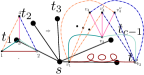
Figure 1. An example of a homological almost-embedding of $K_{4}$ into the plane.

The next ingredient we need is the fact that the classical result about the non-almost-emebddability of the $\lceil d/2\rceil$-skeleton of $(d+2)$-dimensional simplex into $\mathbb{R}^{d}$ holds also in the homological setting.

Theorem 3.3 (Corollary 14 in [GPP⁺17]).

For any $d\geq 0$, the $\lceil d/2\rceil$-skeleton $\Delta_{d+2}^{(\lceil d/2\rceil)}$ of the $(d+2)$-dimensional simplex has no homological almost-embedding in $\mathbb{R}^{d}$.

We note that the proof combines the standard cohomological proof that $\Delta_{2k+2}^{(k)}$ does not almost-embed into $\mathbb{R}^{2k}$ with the fact that cohomology “does not distinguish” between maps and non-trivial chain maps. For details see [GPP⁺17].

3.2. Constrained chain maps

We strengthen the machinery from [GPP⁺17] in order to capture our more general setting. To prove Theorem 2.1, we need one more definition (Definition 3.4). A curious reader may compare our definition of constrained chain map with the definition from [GPP⁺17, Section 3.2]. Let us just remark that the definition presented here is more versatile. (Although it might not be obvious on the first sight.) Unlike the previous definition, the current form allows us to prove the bound on the Radon number. Nevertheless, both definitions are equivalent under some special circumstances.

Let $\mathbf{R}$ be a topological space, let $K$ be a simplicial complex and let $\gamma:C_{*}(K)\to C_{*}(\mathbf{R})$ be a chain map from the simplicial chains of $K$ to the singular chains of $\mathbf{R}$.

Definition 3.4 (Constrained chain map).

Let $\mathcal{F}$ be a family of sets in $\mathbf{R}$ and $P$ be a (multi-)set of points in $\mathbf{R}$. Let $\gamma:C_{*}(K)\to C_{*}(\mathbf{R})$ be the aforementioned chain map. We say that $\gamma$ is constrained by $(\mathcal{F},\Phi)$ if:

1. $\Phi$ is a map from $K$ to $2^{P}$ such that $\Phi(\sigma\cap\tau)=\Phi(\sigma)\cap\Phi(\tau)$ for all $\sigma,\tau\in K$ and $\Phi(\emptyset)=\emptyset$.

2. For any simplex $\sigma\in K$, the support of $\gamma(\sigma)$ is contained in $\operatorname{conv}_{\mathcal{F}}{\Phi(\sigma)}$.

If there is some $\Phi$ such that a chain map $\gamma$ from $K$ is constrained by $(\mathcal{F},\Phi)$, we say that $\gamma$ is constrained by $(\mathcal{F},P$).

Remark 3.

We note that the switch to multisets requires some minor adjustments. If $P=\{p_{i}\mid i\in I\}$ is a multiset, one needs to replace the multiset $P$ by the index set $I$ in all definitions and proofs; and if $J\subseteq I$ consider $\operatorname{conv}_{\mathcal{F}}(J)$ as a shorthand notation for $\operatorname{conv}_{\mathcal{F}}(\{p_{i}\mid i\in J\})$. However, we have decided not to clutter the main exposition with such technical details.

The most important ingredient for the proof of Theorem 2.1 is the following proposition:

Proposition 3.5.

For any finite simplicial complex $K$ and a non-negative integer $b$ there exists a constant $r_{K}(b)$ such that the following holds. For any family $\mathcal{F}$ in a topological space $\mathbf{R}$ with $HC_{\dim K}(\mathcal{F})\leq b$ and any set $P\subseteq\mathbf{R}$ of at least $r_{K}(b)$ points there exists a nontrivial chain map $\gamma:C_{*}(K)\to C_{*}(\mathbf{R})$ that is constrained by $(\mathcal{F},P)$.

Furthermore, if $\dim K\leq 1$, one can even find such $\gamma$ that is induced by some continuous map $f\colon|K|\to\mathbf{R}$ from the geometric realization $|K|$ of $K$ to $\mathbf{R}$.

Before proving Theorems 2.1 and 2.2, let us relate Proposition 3.5 to the Radon number.

Proposition 3.6.

Let $\mathbf{R}$ be a topological space and $K$ a finite simplicial complex that does not homologically almost-embed into $\mathbf{R}$. Then for each integer $b\geq 0$ and every family $\mathcal{F}$ of sets in $\mathbf{R}$ satisfying $HC_{\dim K}(\mathcal{F})\leq b$, the Radon number $r(\mathcal{F})$ is at most $r_{K}(b)$, where $r_{K}(b)$ is the constant from Proposition 3.5.

Moreover, if $\dim K\leq 1$, it suffices to assume that $K$ does not almost-embed into $\mathbf{R}$.

Proof.

If $r(\mathcal{F})>r_{K}(b)$, then there is a set $P$ of $r_{K}(b)$ points such that for any two disjoint subsets $P_{1},P_{2}\subseteq P$ we have $\operatorname{conv}_{\mathcal{F}}(P_{1})\cap\operatorname{conv}_{\mathcal{F}}(P_{2})=\emptyset$. Let $\gamma\colon C_{*}(K)\to C_{*}(\mathbf{R})$ be a nontrivial chain map constrained by $(\mathcal{F},P)$ given by Proposition 3.5. We show that $\gamma$ is a homological almost-embedding of $K$, which will be a contradiction. Indeed, let $\sigma$ and $\tau$ be two disjoint simplices of $K$. The supports of $\gamma(\sigma)$ and $\gamma(\tau)$ are contained, respectively, in $\operatorname{conv}_{\mathcal{F}}\Phi(\sigma)$ and $\operatorname{conv}_{\mathcal{F}}\Phi(\tau)$. By the definition of $\Phi$, $\Phi(\sigma)$ and $\Phi(\tau)$ are disjoint subsets of $P$, hence

$$\operatorname{conv}_{\mathcal{F}}\Phi(\sigma)\cap\operatorname{conv}_{\mathcal{F}}\Phi(\tau)=\emptyset.$$

In other words, $\gamma$ is a homological almost-embedding of $K$, which is the desired contradiction.

If $\dim K\leq 1$, one can take $\gamma$ to be induced by a continuous map $f\colon|K|\to\mathbf{R}$. However, one can easily check that in that case $\gamma$ is a homological almost-embedding if and only if $f$ is an almost-embedding. ∎

Theorems 2.1 and  2.2 are now immediate consequences of Proposition 3.6.

Proof of Theorem 2.1.

By Theorem 3.3, $\Delta_{d+2}^{(\lceil d/2\rceil)}$ does not homologically almost-embed into $\mathbb{R}^{d}$, so Proposition 3.6 applies and yields Theorem 2.1. ∎

Proof of Theorem 2.2.

By results in [GMP⁺17], for each surface $S$ there is a finite graph $G$ that does not almost-embed into $S$, so Proposition 3.6 applies. ∎

We note that compared to [GMP⁺17], recent works by Paták, Tancer [PT19], and Fulek, Kynčl [FK18] provide much smaller graphs which are not almost-embeddable into $S$.

3.3. Combinatorial part of the proof

The classical Ramsey theorem [Ram29] states that for all positive integers $k,n$ and $c$ there is a number $R_{k}(n;c)$ such that the following holds. For each set $X$ satisfying $|X|\geq R_{k}(n;c)$ and each coloring $\rho\colon\binom{X}{k}\to[c]$, there is a monochromatic subset $Y\subseteq X$ of size $n$, where a subset $Y$ is monochromatic, if all $k$-tuples in $Y$ have the same color. We note that a coloring is just another name for a map. However, it is easier to say “the color of $z$”, instead of “the image of $z$ under $\rho$”. Observe that the case $k=1$ corresponds to the pigeon hole principle and $R_{1}(n;c)=n(c-1)+1$.

In order to perform the induction step in the proof of Proposition 3.5, we need the following Ramsey type theorem.

Proposition 3.7.

For any positive integers $k$, $m$, $n$, $c$ there is a constant $N_{k}=N_{k}(n;m;c)$ such that the following holds. Let $X$ be a set and for every $V\subseteq X$ let $\rho_{V}\colon\binom{V}{k}\to[c]$ be a coloring of the $k$-element subsets of $V$. (If $|V|<k$, the coloring $c_{V}$ is, by definition, the empty map.) If $|X|\geq N_{k}$, then there always exists an $n$-element subset $Y\subseteq X$ and a map $M_{(\cdot)}\colon\binom{Y}{m}\to 2^{X\setminus Y}$ such that all the sets $M_{Z}$ for $Z\in\binom{Y}{m}$ are disjoint, and each $Z\in\binom{Y}{m}$ is monochromatic in $\rho_{Z\cup M_{Z}}$.

The fact that each $k$-tuple is colored by several different colorings $\rho_{V}$ reflects the fact that we are going to color a cycle $z$ by the singular homology of $\gamma(z)$ inside $\operatorname{conv}_{\mathcal{F}}\Phi(V)$ for various different sets $V$. It may thus easily happen that if $z,z^{\prime}$ are two cycles with vertices in $V\cap W$, they have the same colors in $V$ but their colors in $W$ are different.

Proof.

Let $r=R_{k}(m;c)$. We claim that it is enough to take

$$N_{k}=R_{r}\left(n+\binom{n}{m}\cdot(r-m);\binom{r}{m}\right).$$

Suppose that $|X|\geq N_{k}$ and choose an arbitrary order of the elements of $X$.

By the choice of $r$, if $V\in\binom{X}{r}$, then there is a subset $A\subseteq V$ of size $m$ such that $\rho_{V}$ assigns the same color to all $k$-tuples in $A$. Let us introduce another coloring $\eta$ that colors each $V\in\binom{X}{r}$ by the relative position of the first monochromatic $m$-tuple $A$ inside $V$ (with respect to the lexicographic ordering). In total, there are $\binom{r}{m}$ colors.

For illustration: If $V=\{2,4,6,8,10,12,14,16,18\}$ and $A=\{2,4,14,16\}$ we assign $V$ the “color” $\{1,2,7,8\}$, since the elements of $A$ are on first, second, 7th and 8th position of $V$.

Since $|X|\geq N_{k}$, there is a subset $U$ of size $n+\binom{n}{m}\cdot\left(r-m\right)$, such that all $r$-tuples in $U$ have the same color in $\eta$, say color $\Omega$.

Consider the set $Y^{\prime}=\{1,2,\ldots,n\}$. Since the rational numbers are dense, we can find an assignment

$$N\colon\binom{Y^{\prime}}{m} \to \binom{\mathbb{Q}\setminus Y^{\prime}}{r-m}$$

$$Z^{\prime} \mapsto N_{Z^{\prime}}$$

of mutually disjoint sets $N_{Z^{\prime}}$ such that $Z^{\prime}$ has position $\Omega$ within the set $Z^{\prime}\cup N_{Z^{\prime}}$.

The unique order-preserving isomorphism from $Y^{\prime}\cup\bigcup N_{Z^{\prime}}$ to $U$ then carries $Y^{\prime}$ to the desired set $Y$ and $N_{Z^{\prime}}$ to the desired sets $M_{Z}$. ∎

3.4. The induction

Proof of Proposition 3.5.

We proceed by induction on $\dim K$, similarly as in [GPP⁺17]. If the reader finds the current exposition too fast, we encourage him/her to consult [GPP⁺17] which goes slower and shows motivation and necessity of some ideas presented here. Note however, that our current setup is more general as it works for an arbitrary closure space (for definition see Appendix A).

Induction basis. If $K$ is $0$-dimensional with vertices $V(K)=\{v_{1},\ldots,v_{m}\}$, we set $r_{K}(b)=m$. If $P=\{x_{1},\ldots,x_{n}\}$ is a point set in $\mathbf{R}$ with $|P|\geq m$, we can take as $\Phi$ the map $\Phi(v_{i})=\{x_{i}\}$. It remains to define $\gamma$. We want it to “map” $v_{i}$ to $x_{i}$. However, $\gamma$ should be a chain map from simplicial chains of $K$ to singular chains in $\mathbb{R}^{d}$. Therefore for each vertex $v_{i}$ we define $\gamma(v_{i})$ as the unique map from $\Delta_{0}$ to $x_{i}$ (here we consider $\Delta_{n}$ to be a geometric simplex.); and extend this definition linearly to the whole $C_{0}(K)$. By construction, $\gamma$ is nontrivial and constrained by $(\mathcal{F},\Phi)$.

Induction step. Let $\dim K=k\geq 1$. The aim is to find a chain map $\gamma\colon C_{*}(K^{(k-1)})\to C_{*}(\mathbf{R})$ and a suitable map $\Phi$ such that $\gamma$ is nontrivial, constrained by $(\mathcal{F},\Phi)$ and $\gamma(\partial\sigma)$ has trivial homology inside $\operatorname{conv}_{\mathcal{F}}\Phi(\sigma)$ for each $k$-simplex $\sigma\in K$. Extending such $\gamma$ to the whole complex $K$ is then straightforward.

Let $s\geq 1$ be some integer depending on $K$ which we determine later. To construct $\gamma$ we will define three auxiliary chain maps

$$C_{*}\left(K^{(k-1)}\right)\quad\xrightarrow{\makebox[20.00003pt]{$\alpha$}}\quad C_{*}\left((\operatorname{sd}K)^{(k-1)}\right)\quad\xrightarrow{\makebox[30.00005pt]{$\beta$}}\quad C_{*}\left(\Delta_{s}^{(k-1)}\right)\xrightarrow{\makebox[20.00003pt]{$\gamma^{\prime}$}}\quad C_{*}(\mathbf{R}),$$

where $\operatorname{sd}K$ is the barycentric subdivision of $K$.

Definition of $\alpha$. We start with the easiest map, $\alpha$. It maps each $l$-simplex $\sigma$ from $K^{(k-1)}$ to the sum of the $l$-simplices in the barycentric subdivision of $\sigma$.

Definition of $\gamma^{\prime}$. The map $\gamma^{\prime}$ is obtained from induction. Let the cardinality of $P$ be large enough. Since $\dim\Delta_{s}^{(k-1)}=k-1$, by induction hypothesis, there is a nontrivial chain map $\gamma^{\prime}:C_{*}(\Delta_{s}^{(k-1)})\to C_{*}(\mathbf{R})$ and a map $\Psi\colon\Delta_{s}^{(k-1)}\to 2^{P}$ such that $\gamma^{\prime}$ is constrained by $(\mathcal{F},\Psi)$.

In order to define $\Phi$ easily later on, we extend $\Psi$ to $\Delta_{s}$. For $\sigma\in\Delta_{s}$ we define

(1) $$\Psi(\sigma)=\bigcup_{\tau\in\Delta_{s}^{(k-1)},\tau\subseteq\sigma}\Psi(\tau).$$

If $\tau\subseteq\sigma\in\Delta_{s}^{(k-1)}$, then $\Psi(\tau)\cap\Psi(\sigma)$ is equal to $\Psi(\tau\cap\sigma)=\Psi(\tau)$. Thus the equality (1) does not change the value of $\Psi(\sigma)$ if $\sigma\in\Delta_{s}^{(k-1)}$ and it is indeed an extension of $\Psi$. Moreover, easy calculation shows that $\Psi(A)\cap\Psi(B)=\Psi(A\cap B)$ for any $A,B\in\Delta_{s}$.

Definition of $\beta$. With the help of Proposition 3.7 it is now easy to find the map $\beta$. Indeed, for each simplex $\tau\in\Delta_{s}$, let $c_{\tau}$ be the coloring that assigns to each $k$-simplex $\sigma\subseteq\tau$ the singular homology class of $\gamma^{\prime}(\partial\sigma)$ inside $\operatorname{conv}_{\mathcal{F}}(\Psi(\tau))$. Let $m$ be the number of vertices of $\operatorname{sd}\Delta_{k}$, $n$ the number of vertices of $\operatorname{sd}K$ and $c$ the maximal number of elements in $\widetilde{H}_{k}(\bigcap\mathcal{G};\mathbb{Z}_{2})$, where $\mathcal{G}\subseteq\mathcal{F}$. Clearly $c\leq 2^{b}$.

Thus if $s\geq N_{k+1}(n;m;c)$ from Proposition 3.7, the following holds.

1. There is an inclusion $j$ of $\left(\operatorname{sd}K\right)^{(k-1)}$ to a simplex $Y\subseteq\Delta_{s}$. We let $\varphi\colon K\to 2^{V(\Delta_{s})}$ be the map that to each $\sigma\in K$ assigns the set $j(V(\operatorname{sd}\sigma))$. In particular, $\varphi(\sigma)\subseteq Y$ for each $\sigma\in K$.

2. For each $k$-simplex $\mu$ in $K$ there is a simplex $M_{\mu}$ in $\Delta_{s}$ with the following three properties:

   1. For all $k$-simplices $\tau$ inside $\operatorname{sd}\mu$, the singular homology class of $\gamma^{\prime}(j(\partial\tau))$ inside $\operatorname{conv}_{\mathcal{F}}\Psi(M_{\mu}\cup\varphi(\mu))$ is the same,

   2. each $M_{\mu}$ is disjoint from $Y$,

   3. all the simplices $M_{\mu}$ are mutually disjoint.

We define $M_{\mu}:=\emptyset$ for $\mu\in K$ a simplex of dimension at most $k-1$. We set $\Phi(\mu):=\Psi(M_{\mu}\cup\varphi(\mu))$. Note that for a simplex $\sigma\in K^{(k-1)}$, $\Phi(\sigma)$ reduces to $\Psi(\varphi(\sigma))$.

Let $\beta$ be the chain map induced by $j$. Observe that $\Phi$ satisfies $\Phi(\emptyset)=\emptyset$ and $\Phi(A\cap B)=\Phi(A)\cap\Phi(B)$, $A,B\in K$. Indeed, the first claim is obvious and for the second one let $\sigma,\tau$ be distinct simplices in $K$:

$$\Phi(\mu)\cap\Phi(\tau) =\Psi\left(M_{\mu}\cup\varphi(\mu)\right)\cap\Psi\left(M_{\tau}\cup\varphi(\tau)\right)=\Psi\left([M_{\mu}\cup\varphi(\mu)]\cap[M_{\tau}\cup\varphi(\tau)]\right)$$

$$=\Psi(\varphi(\mu)\cap\varphi(\tau)),$$

where the second equality express the fact that $\Psi$ respects intersections and the last equality uses 2(ii), 2(iii) and the fact that $\varphi(\sigma)\subseteq Y$ for every $\sigma\in K$. Then

$$\Phi(\mu)\cap\Phi(\tau)=\Psi(\varphi(\mu)\cap\varphi(\tau))=\Psi(\varphi(\mu\cap\tau))=\Phi(\mu\cap\tau)$$

since $\varphi$ obviously respects intersections and $\dim(\mu\cap\tau)\leq k-1$.

We define $\gamma$ on $K^{(k-1)}$ as the composition $\gamma^{\prime}\circ\beta\circ\alpha$. Then, by the definition, $\gamma$ is a nontrivial chain map constrained by $(\mathcal{F},\Phi)$.

As the last step, we extend $\gamma$ to the whole complex $K$. If $\sigma$ is a $k$-simplex of $K$, all the $k$-simplices $\zeta$ in $\operatorname{sd}\sigma$ have the same value of $\gamma^{\prime}\beta(\partial\zeta)$ inside $\operatorname{conv}_{\mathcal{F}}\Phi(\sigma)$. Since there is an even number of them and we work with $\mathbb{Z}_{2}$-coefficients, $\gamma(\partial\sigma)$ has trivial homology inside $\operatorname{conv}_{\mathcal{F}}\Phi(\sigma)$. So for each such $\sigma$ we may pick some $\gamma_{\sigma}\in C_{k}\left(\operatorname{conv}_{\mathcal{F}}\Phi(\sigma);\mathbb{Z}_{2}\right)$ such that $\partial\gamma_{\sigma}=\gamma(\partial\sigma)$ and extend $\gamma$ by setting $\gamma(\sigma):=\gamma_{\sigma}$. Then, by definition, $\gamma$ is a non-trivial chain map from $C_{*}(K;\mathbb{Z}_{2})$ to $C_{*}(\mathbf{R};\mathbb{Z}_{2})$ constrained by $(\mathcal{F},\Phi)$ and hence by $(\mathcal{F},P)$.

It remains to show that if $\dim K\leq 1$, we can take $\gamma$ that is induced by a continuous map $f\colon|K|\to\mathbf{R}$. If $\dim K=0$, we map each point to a point, so the statement is obviously true.

If $\dim K=1$, we inspect the composition $\gamma=\gamma^{\prime}\circ\beta\circ\alpha$. It maps points of $K$ to points in $\mathbf{R}$ in such a way that the homology class of $\gamma(\partial\tau)$ inside $\operatorname{conv}_{\mathcal{F}}(\Psi(\tau))$ is trivial for each edge $\tau$ of $K$. But this means that the endpoints of $\tau$ get mapped to points in the same path-connected component of $\operatorname{conv}_{\mathcal{F}}(\Psi(\tau))$ and can be connected by an actual path. ∎

4. A fractional Helly theorem on surfaces

In order to prove Theorem 2.5, we need to bring the constant $m$ from Theorem 2.3 (applied to a surface $S$) down to three for $b=0$ and to $2b+4$ for $b\geq 1$, respectively. The presented method is based on the recent result of Kalai and the author [KP20] and allows us to significantly decrease $m$ to a small value as soon as we have a finite upper bound.

We need few definitions first. Let $\mathcal{A}=\{A_{1},\ldots,A_{n}\}$ be subsets of a surface $S$. Set $A_{I}=\bigcap_{i\in I}A_{i}$ and let $N(\mathcal{A})=\{I\in[n]\colon A_{I}\neq\emptyset\}$ be the nerve of $\mathcal{A}$. We put $f_{k}(\mathcal{A})=|\{I\in N(\mathcal{A})\colon|I|=k+1\}|$. In words, $f_{k}$ counts the number of intersecting $(k+1)$-tuples from $\mathcal{A}$.

The main tool for the bootstrapping is the following proposition.

Proposition 4.1.

Let $b\geq 0$ and $k\geq 2$ be integers satisfying that for $b=0$, $k\geq 2$, and for $b\geq 1$, $k>2b+2$, respectively. Let $S$ be a surface. Then for every $\alpha\in(0,1)$ there exists $\alpha^{\prime}=\alpha^{\prime}(\alpha,b,k,S)>0$ such that for any sufficiently large family $\mathcal{A}$ of $n$ open sets in $S$ with $HC_{1}(\mathcal{A})\leq b$ and every integer $r\geq 1$, the following holds:

(2) $$f_{k}(\mathcal{A})\geq\alpha\binom{n}{k+1}\quad\Rightarrow\quad f_{k+r}(\mathcal{A})\geq\alpha^{\prime}\binom{n}{k+r+1}.$$

Proof of Theorem 2.5.

Let $b\geq 0$ and let $k_{0}=k_{0}(b)$ be an integer depending on $b$. Namely, we set $k_{0}(0)=3$ and $k_{0}(b)=2b+4$ for $b\geq 1$. Let $m$ be the value from the (non-optimal) fractional Helly theorem (Theorem 2.3). We assume that $m\geq k_{0}+1$, otherwise we just take a minimal integer which satisfies both conditions. By Proposition 4.1 ($k=k_{0}-1,r=m-k_{0}$) we get that if at least an $\alpha$-fraction of all $k_{0}$-tuples intersect, then also some $\alpha^{\prime}$-fraction of all $m$-tuples intersect. Theorem 2.3 now implies that there is a point common to some $\beta$-fraction of all the sets. This finishes the proof. ∎

It remains to prove Proposition 4.1. As mentioned, this proof heavily relies on [KP20, Theorem 2.3], which can be reformulated, for open sets and in terms of bounded homological complexity, as follows:

Theorem 4.2 ([KP20]).

Let $S$ be a surface, $b\geq 0$ an integer and let $k=k(b)$ be an integer depending on $b$, namely $k(0)\geq 2$ and $k(b)>2b+2$ for $b\geq 1$. Then there exist constants $c_{1}>0,c_{2}\geq 0$ depending only on $k,b$ and $S$ such that the following holds. Let $\mathcal{A}$ be a finite family of open sets in $S$ with $HC_{1}(\mathcal{A})\leq b$. Then

$$f_{k}(\mathcal{A})>c_{1}f_{k-1}(\mathcal{A})+c_{2}\quad\Rightarrow\quad f_{k+1}(\mathcal{A})>0.$$

Since a nerve of any family is a simplicial complex, hence a hypergraph, we will recall some useful facts about hypergraphs.

Hypergraphs. A hypergraph is $\ell$-uniform if all its edges have size $\ell$. A hypergraph is $\ell$-partite, if its vertex set $V$ can be partitioned into $\ell$ subsets $V_{1},\ldots,V_{\ell}$, called classes, so that each edge contains at most one point from each $V_{i}$. Let $K^{\ell}(t)$ denote the complete $\ell$-partite $\ell$-uniform hypergraph with $t$ vertices in each of its $\ell$ vertex classes.

We need the following theorem of Erdős and Simonovits [ES83] about super-saturated hypergraphs (see also [Mat02, Chapter 9.2]):

Theorem 4.3 ([ES83]).

For any positive integers $\ell$ and $t$ and any $\varepsilon>0$ there exists $\delta>0$ with the following property: Let $H$ be an $\ell$-uniform hypergraph on $n$ vertices and with at least $\varepsilon\binom{n}{\ell}$ edges. Then $H$ contains at least $\delta n^{\ell t}$ copies of $K^{\ell}(t)$.

Proof of Proposition 4.1.

Let $\mathcal{A}=\{A_{1},\ldots,A_{n}\}$ be a family of sets in $S$ satisfying the assumptions. Since $f_{k-1}(\mathcal{A})\leq\binom{n}{k}$, Theorem 4.2 gives

(3) $$f_{k}(\mathcal{A})>c_{1}\binom{n}{k}+c_{2}\quad\Rightarrow\quad f_{k+1}(\mathcal{A})>0,$$

for some constants $c_{1}>0,c_{2}\geq 0$.

Note that it is enough to show (2) for $r=1$ as the rest can be obtained by induction.

Let $H$ be a $(k+1)$-uniform hypergraph whose vertices and edges correspond to the vertices and $k$-simplices of the nerve $N$ of $\mathcal{A}$. By assumption $H$ has at least $\alpha\binom{n}{k+1}$ edges. Set

$$t:=\left\lceil\frac{c_{1}(k+1)^{k}}{k!}+c_{2}\right\rceil$$

By Theorem 4.3 ($\varepsilon=\alpha,\ell=k+1$), there is at least $\delta n^{(k+1)t}$ copies of $K^{k+1}(t)$ in $H$.

Since $K^{k+1}(t)$ has $(k+1)t$ vertices and $t^{k+1}$ edges, it follows by (3) that for every copy of $K^{k+1}(t)$ in $H$ there is an intersecting subfamily of size $k+2$ among the corresponding members of $\mathcal{A}$. Indeed, the implication (3) translates into checking that for $k\geq 2$, $t\geq 1$,

$$t^{k+1} > c_{1}\binom{(k+1)t}{k}+c_{2}.$$

On the other hand, each such intersecting $(k+2)$-tuple is contained in at most $n^{(k+1)t-(k+2)}$ distinct copies of $K^{k+1}(t)$ (we count the number of choices for the vertices not belonging to the considered $(k+2)$-tuple), and the result follows, i.e. $f_{k+1}(\mathcal{A})\geq\delta n^{k+2}\geq\alpha^{\prime}\binom{n}{k+2}$. ∎

5. Discussion

Qualitative sharpness of Theorem 2.1.

Example 1.

The bound on the Radon number provided by Theorem 2.1 is extremly large as it is obtained by an iterative application of Ramsey theorem. Nevertheless, the result is optimal in the following sense: all $\widetilde{\beta}_{i}$, $0\leq i<\lceil\frac{d}{2}\rceil$, need to be bounded in order to have a bounded Radon number. Indeed, fix $0\leq k<\lceil\frac{d}{2}\rceil$ and let $n$ be arbitrarily large. Let $K$ be a realization of the $k$-skeleton of the $(n-1)$-dimensional simplex in $\mathbb{R}^{d}$ (see [Mat03, Section 1.6]); more precisely, let $V(K)=\{v_{1},\ldots,v_{n}\}$ be a set of $n$ points in general position in $\mathbb{R}^{d}$, then each subset $A\subseteq V(K)$ of size at most $k+1$ spans a geometric simplex $\operatorname{conv}A$. Here $\operatorname{conv}(\cdot)$ stands for the standard convex hull in $\mathbb{R}^{d}$. For each $i\in[n]$, let $F_{i}$ be the union of all simplices in $K$ not containing the vertex $v_{i}$, put $\mathcal{F}=\{F_{i}\colon i\in[n]\}$. We show that $r(\mathcal{F})>n$. More precisely, we show that for any two disjoint subsets $B_{1},B_{2}\subseteq V(K)$ we have $\operatorname{conv}_{\mathcal{F}}(B_{1})\cap\operatorname{conv}_{\mathcal{F}}(B_{2})=\emptyset$. Observe that for $C\subsetneq[n]$, $\operatorname{conv}_{\mathcal{F}}\{v_{i}\colon i\in C\}$ is the induced subcomplex of $K$ spanned by the vertices $\{v_{i}\colon v_{i}\in C\}$ as $\operatorname{conv}_{\mathcal{F}}\{v_{i}\colon i\in C\}=\bigcap_{i\in[n]\setminus C}F_{i}$. This implies that that $r(\mathcal{F})>n$ as in any partition of $V(K)$ the convex hulls of the parts cannot intersect. Given a subfamily $\mathcal{G}\subseteq\mathcal{F}$ of cardinality $m$ ($m\leq n$), $\bigcap\mathcal{G}$ is the $k$-skeleton of a simplex on $n-m$ vertices, and hence have all reduced Betti numbers equal to zero except in dimension $k$, where the reduced Betti number equals $\binom{n-m}{k+1}$.

This construction has been used before ([GPP⁺17, Example 3]) to show that all $\widetilde{\beta}_{i}$, $0\leq i<\lceil\frac{d}{2}\rceil$, have to be bounded in order to have a bounded Helly number.

$\mathbb{Z}_{2}$-coefficients and manifolds. A curious reader might wonder why do we compute over $\mathbb{Z}_{2}$. Could we possibly get a better bound using another ring like $\mathbb{Z}$ or $\mathbb{Z}_{p}$?

First reason is that so far the homological van Kampen-Flores theorem (Theorem 3.3) is proven only for $\mathbb{Z}_{2}$. Using ideas from Özaydin’s paper [Ö87], it would be possible to prove an analogous result over $\mathbb{Z}_{p}$, but then we would need to consider a $(1-1/p)d$-dimensional complex in Proposition 3.6. Since raising the target dimension by one requires twofold application of Ramsey theorem, such procedure is unlikely to improve the resulting bound on the Radon number. Moreover, one would need to restrict the homological complexity up to that dimension. In other words, it would not be enough to bound the complexity only up to mid-level. Nevertheless, there still might be rare situations in which such approach results in slightly better bounds on Tverberg numbers than the ones that follow from combination of Theorem A.6 and our bound on Radon number.

The second reason is that the choice of $\mathbb{Z}_{2}$ enables us to completely separate the Ramsey argument (that is, no homology is involved in Proposition 3.7). One big advantage of having the topological and combinatorial parts of the proof independent is that once there is an extension of the homological van Kampen-Flores theorem to manifolds, we readily get most of the results in this paper also for families on manifolds.

Problem 4.

Is there a homological van Kampen-Flores theorem for manifolds?

It might seem that the need for a homological van Kampen-Flores for manifolds can be overcome by the approach mentioned in Section 2.1, as we can often embed any reasonably nice $d$-manifold into $\mathbb{R}^{2d}$. For example, combining the embedding with Theorems 2.1 and A.8, we get a $(p,q)$-theorem for manifolds. However, $p\geq m$ has to be sufficiently large as the bound $m$ on the fractional Helly number is large. Moreover, we need to bound homological complexity of $\mathcal{F}$ up to level $d$. This brings a question, can we improve the bound on the Radon number?

Problem 5.

Provide lower and upper bounds on the Radon number from Theorem 2.1.

This would be helpful not only from the perspective of the manifolds, but also for the fractional Helly theorems, as the dependency on the Radon number is hidden in the bound on $\beta$ in Theorem 2.5. Indeed, Radon number tells us how many steps in the bootstraping described in Section 4 we need to perform.

What our method gives, regarding Problem 5, are the following partial results.

Theorem 5.1.

For $\mathcal{F}\subseteq\mathbb{R}^{d}$ with $HC_{\lceil d/2\rceil}(\mathcal{F})=0$ the Radon number $r(\mathcal{F})$ is at most $d+3$. In case that $HC_{d}(\mathcal{F})=0$, we have that $r(\mathcal{F})\leq d+2$. Moreover, the first bound is sharp for $d\geq 2$, whereas the second bound is sharp for $d\geq 0$.

Proof.

In both cases we proceed exactly as in the proof of Theorem 2.1, the only difference is that we do not need to use Ramsey theorem and barycentric subdivisions. More precisely we identify the points of the constructed complex with the original point set $P$ and set $\Psi(\sigma)=\sigma$ for every face of the constructed complex. In the induction procedure, the boundary of each simplex $\partial\tau$ lies in the set $\operatorname{conv}_{\mathcal{F}}(\sigma)$, which is homologically trivial and hence can be “filled” by some cycle. Thus in the first case we manage to construct a non-trivial chain map from $\Delta_{d+2}^{(\lceil d/2\rceil)}$ to $\mathbb{R}^{d}$ constrained by $(\mathcal{F},P)$. The rest of the proof is the same, we use Theorem 3.3 in combination with Proposition 3.6.

In the second case we construct a non-trivial chain map from the boundary of $(d+1)$-simplex (which is $\Delta_{d+1}^{(d)}$) to $\mathbb{R}^{d}$ constrained by $(\mathcal{F},P)$. By [GPP⁺17, Lemma 15], this simplicial complex admits no homological almost-embedding into $\mathbb{R}^{d}$, so Proposition 3.6 yields the result.

It remains to show the sharpness. The case $HC_{d}(\mathcal{F})=0$ is simple, take as $\mathcal{F}$ the family of all $(d-1)$-faces of the $d$-simplex $\Delta_{d}$. $\mathcal{F}$ clearly has a geometric realization in $\mathbb{R}^{d}$, $TC_{d}(\mathcal{F})=0$ as all sets are convex, and $r(\mathcal{F})>d+1$ as $\operatorname{conv}_{\mathcal{F}}G=\operatorname{conv}G$ for any $G\subsetneq V(\Delta_{d})$. Note that this is the classical example that Radon theorem of standard convex sets is tight.

Now we construct a family $\mathcal{F}$ with $HC_{\lceil d/2\rceil}(\mathcal{F})=0$ and $r(\mathcal{F})>d+2$. The construction and its analysis is similar to the one in Example 1. Let $K$ be the $(d-1)$-skeleton of the $(d+1)$-simplex $\Delta_{d+1}$ on the vertex set $V(K)=\{v_{1},\ldots,v_{d+2}\}$. We show that $K$ can be realized in $\mathbb{R}^{d}$. We start with a (geometric) $d$-simplex $\Delta_{d}$ in $\mathbb{R}^{d}$, say with vertices $V(K)\setminus\{v_{d+2}\}$. Now we consider the barycenter $v_{d+2}$ of $\Delta_{d}$ and take the $(d-1)$-skeleton of stellar subdivision $(\partial\Delta_{d}*v_{d+2})$. What we get is a realization of $K$ in $\mathbb{R}^{d}$. Let $\mathcal{F}=\{F_{i}\colon i\in[d+2]\}$, where $F_{i}$ is a union of all faces of $K$ not containing the vertex $v_{i}$. In other words, $F_{i}$’s are the boundaries of $d$-faces of $\Delta_{d+1}$. Note that $r(\mathcal{F})>d+2$ from exactly the same reasons as before. Given a subfamily $\mathcal{G}\subsetneq\mathcal{F}$ of cardinality $m\geq 2$, $\bigcap\mathcal{G}$ is a $(d+1-m)$-simplex, hence it has all reduced Betti numbers trivial. If $|\bigcap\mathcal{G}|=1$, i.e. $\mathcal{G}=F_{i}$, we have that all $\tilde{\beta}_{j}(F_{i})=0$ for $0\leq j\leq d-2$ and $\tilde{\beta}_{d-1}(F_{i})=1$ as $F_{i}$ is the boundary of $d$-simplex. As $d>\lceil d/2\rceil$ for $d\geq 2$, we conclude that $TC_{\lceil d/2\rceil}(\mathcal{F})=0$. ∎

Funding. The work was supported by Charles University projects UNCE/SCI/022 and PRIMUS/21/SCI/014.

Acknowledgements. I am very grateful to Pavel Paták for numerous discussions, helpful suggestions and proofreadings. Many thanks to Xavier Goaoc for his feedback and comments, which have been very helpful in improving the overall presentation. I would also like to thank to Endre Makai for pointers to relevant literature, especially to the book [Sol84], and Natan Rubin for several discussions at the very beginning of the project.

Appendix A Appendix – General set systems

The purpose of this appendix is to clarify the confusion about convexity spaces and $\mathcal{F}$-hulls. Many authors, especially in combinatorics, seem to use the stronger notion of convexity space, even when they result hold in greater generality for arbitrary closure system. Since some authors use one definition and the others a different one, this creates an unnecessary tension. In this appendix we try to explain the difference between these two notions. Moreover, we show that when dealing with finite set systems, a theorem for convexity space is valid if and only if its $\mathcal{F}$-hull analogue is true. This is not true for infinite set systems. In order to achieve this goal we shall relate the concept of $\mathcal{F}$-hull and the concept of convexity space. This will allow us to reformulate a recent result of Holmsen and Lee [HL21, Thm 1.1] to the form that a family $\mathcal{F}$ with bounded Radon number has a fractional Helly property. Revisiting the paper of Alon et al. [AKMM02] gives the existence of weak-epsilon nets or $(p,q)$-theorem for families with bounded Radon number. Since by our main theorem families with bounded homological complexity have bounded Radon number, we immediately get these theorems as well.

We start with defining a convexity space.

Definition A.1.

A pair $(X,\mathcal{C})$, where $X$ is an underlying (non-empty) set and $\mathcal{C}$ is a family of subsets of $X$ is called a convexity space if it satisfies the following conditions:

1. $\emptyset,X\in\mathcal{C}$,

2. $\mathcal{C}$ is closed under taking intersections, that is $\bigcap\mathcal{G}\in\mathcal{C}$ for any non-empty $\mathcal{G}\subseteq\mathcal{C}$,

3. $\mathcal{C}$ is closed under taking nested unions of chains, that is $\bigcup_{G\in\mathcal{G}}G\in\mathcal{C}$ for any non-empty $\mathcal{G}=\{G_{1}\subseteq G_{2}\subseteq\cdots\}\subseteq\mathcal{C}$.

The sets in $\mathcal{C}$ are called convex sets. Note that the last condition is trivially satisfied whenever $\mathcal{C}$ is finite. For this reason people in combinatorics often omit the last condition in the definition of convexity space. This is not correct as the standard name for a space that satisfies the first two conditions is a closure space or a closure system [vdV93].

The prototypical example of convexity space is the standard Euclidean convexity $(\mathbb{R}^{d},\mathcal{C}^{d})$, where $\mathcal{C}^{d}$ is the family of all convex sets in $\mathbb{R}^{d}$.

We note that for our considerations we will be mostly interested in the second condition together with the assumption that $X$ itself is convex. The condition (iii) and the assumption that $\emptyset\in\mathcal{C}$ are mainly used when the underlying space is a topological space and when we need to guarantee that convex sets behave well with respect to limits (for example in functional analysis). The condition (iii) also provides an “inner” description of convex sets, which we describe in the next paragraph. For more background on convexity spaces we refer to [vdV93], [KW71], [Sol84].

Let $(X,\mathcal{C})$ be a convexity space. We will use the convention that $\bigcap\emptyset=X$. For any $S\subseteq X$, the convex hull of $S$ is defined as the intersection of all convex sets containing $S$, that is $\operatorname{conv}_{\mathcal{C}}(S)=\bigcap\{A\in\mathcal{C}\colon S\subseteq A\}$. It follows from (i) and (ii) that $\operatorname{conv}(S)$ is the minimal (with respect to inclusion) convex set containing $S$. The condition (iii) is needed in order to show that for each point in the convex hull of $A$ there is a finite subset $B\subseteq A$ such that $x$ already lies in the convex hull of $B$ [vdV93, Chapter I, Theorem 1.3]; this is called an inner description. Note that the definition of convex hull coincides with the definition of $\mathcal{C}$-hull from the introduction.

Radon number of a convexity space $(X,\mathcal{C})$ is a Radon number with respect to the family $\mathcal{C}$. We will denote it by $r(\mathcal{C})$. Similarly, Helly number of $(X,\mathcal{C})$ is a Helly number with respect to $\mathcal{C}$ and is denoted by $h(\mathcal{C})$.

We note that the Radon number is monotone: $\mathcal{F}\subseteq\mathcal{G}$ implies that $r(\mathcal{F})\leq r(\mathcal{G})$. This is true since $\operatorname{conv}_{\mathcal{F}}S\supseteq\operatorname{conv}_{\mathcal{G}}S$ for any set $S$.

As one easily verifies, if $X$ is a set, any intersection of convexity spaces on $X$ is again a convexity space. Thus for any family $\mathcal{F}$ of subsets of $X$, there is the smallest convexity space $(X,\mathcal{C})$ for which $\mathcal{F}\subseteq\mathcal{C}$. We say that the convexity space is generated by $\mathcal{F}$, or that $\mathcal{F}$ is the base of $(X,\mathcal{C})$.

Theorem A.2.

Let $X$ be a set and $\mathcal{F}$ a family of subsets of $X$ with $\bigcap\mathcal{F}=\emptyset$. Let $(X,\mathcal{C})$ be the convexity space generated by $\mathcal{F}$. Then $r(\mathcal{C})=r(\mathcal{F})$.

Proof.

If $\bigcap\mathcal{F}=\emptyset$, then $\mathcal{F}^{\cap}:=\left\{\bigcap\mathcal{H}\colon\mathcal{H}\subseteq\mathcal{F}\right\}$ is a closure space. Here we use the convention that $\bigcap\emptyset=X$. Clearly, $\mathcal{F}^{\cap}$ also generates $\mathcal{C}$. Thus if $S\subseteq X$ is an arbitrary finite set, $\operatorname{conv}_{\mathcal{F}}(S)=\operatorname{conv}_{\mathcal{F}^{\cap}}(S)=\operatorname{conv}_{\mathcal{C}}(S)$, where the last equality is [vdV93, Chapter I, Proposition 1.7.2].

If $r(\mathcal{F})=\infty$, the statement is obviously true because of monotonicity of Radon number. Hence we can assume that $r(\mathcal{F})<\infty$, so in the definition of Radon number we use only finite sets, and on these sets all three hulls coincide, Radon numbers of all the families must coincide as well. In other words, we have obtain the desired equalities $r(\mathcal{F})=r(\mathcal{F}^{\cap})=r(\mathcal{C})$. ∎

A.1. Classical theorems revisited

Convexity spaces with bounded Radon number have several further interesting properties. Theorem A.2 enables us to restate such results in terms of families of sets. We list here a translation of several such classical geometric results. In the following $X$ will denote a (non-empty) ground set and $\mathcal{F}$ a family of subsets of $X$. The general concept is as follows: first realize that the statements are trivially satisfied if $\bigcap\mathcal{F}\neq\emptyset$. If $\bigcap\mathcal{F}=\emptyset$, the Radon numbers of $\mathcal{F}$ and of the convexity space generated by $\mathcal{F}$ coincide by Theorem A.2, so apply the relevant theorem for convexity spaces and translate it back to $\mathcal{F}$ using the fact that all sets from $\mathcal{F}$ lie in the convexity space.

Helly-type theorems.

It is a folklore that bounded Radon number implies bounded Helly number, for convexity spaces it was shown in 50’s by Levi. More surprisingly, recent results of Holmsen and Lee show that any convexity space with bounded Radon number has a fractional Helly property as well as enjoys a weak colorful Helly theorem. As promised, we restate these results here in terms of a family $\mathcal{F}$.

Theorem A.3 ([Lev51]).

For any family $\mathcal{F}$ of subsets of $X$ with $\bigcap\mathcal{F}=\emptyset$, we have $h(\mathcal{F})+1\leq r(\mathcal{F})$.

We prove this theorem for an illustration.

Proof.

As $\bigcap\mathcal{F}=\emptyset$, Theorem A.2 gives that $r(\mathcal{F})=r(\mathcal{C})\geq h(\mathcal{C})+1$, where the inequality is the original Levi’s theorem [Lev51]. The fact that $h(\mathcal{C})\geq h(\mathcal{F})$ can be showed either directly, or it follows from [vdV93, Chapter II, Theorem 1.10]. ∎

Theorem A.4 (fractional Helly, [HL21, Thm 1.1]).

For every $r\geq 3$ and $\alpha\in(0,1)$ there exist an $m=m(r)$ and a $\beta=(\alpha,r)\in(0,1)$ with the following property: Let $\mathcal{F}$ be any family of subsets of $X$ with Radon number at most $r$ and let $\mathcal{G}$ be a finite subfamily of $\mathcal{F}$ of $n\geq m$ sets. If at least $\alpha\binom{n}{m}$ of the $m$-tuples of $\mathcal{G}$ have non-empty intersection, then there are at least $\beta n$ members of $\mathcal{G}$ whose intersection is non-empty.

Theorem A.5 (weak colorful Helly, [HL21, Thm 2.2]).

For every integer $r\geq 3$ there exists an integer $m=m(r)$ with the following property: Let $\mathcal{F}$ be a family with Radon number at most $r$. Let $\mathcal{F}_{1},\dots,\mathcal{F}_{m}$ be non-empty finite subfamilies of $\mathcal{F}$. If $\bigcap_{i=1}^{m}S_{i}\neq\emptyset$ for all $S_{i}\in\mathcal{F}_{i}$ and $i\in[m]$, then for some $1\leq i\leq m$ we have $\bigcap_{S\in\mathcal{F}_{i}}S\neq\emptyset$.

Tverberg-type theorems.

We recall that Tverberg number generalizes Radon number in the sense that we seek a partition into $k\geq 3$ disjoint parts whose $\mathcal{F}$-hulls intersect. (for precise definition see Section 2.2). Tverberg number of a convexity space $(X,\mathcal{C})$ is a Tverberg number with respect to the family $\mathcal{C}$ and is denoted by $r_{k}(\mathcal{C})$.

As the Radon number, Tverberg number is also monotone, i.e. $r_{k}(\mathcal{F})\leq r_{k}(\mathcal{G})$ whenever $\mathcal{F}\subseteq\mathcal{G}$. The same reasoning as in the proof of Theorem A.2 gives that for a family $\mathcal{F}\subseteq X$ with $\bigcap\mathcal{F}=\emptyset$, we have $r_{k}(\mathcal{F})=r_{k}(\mathcal{C})$ where $(X,\mathcal{C})$ is the convexity space generated by $\mathcal{F}$.

Theorem A.6 ([JW81, Pá22]).

Let $\mathcal{F}$ be a family of subsets of $X$ with a finite Radon number $r$. Then, for $k\geq 2$,

• $r_{k}(\mathcal{F})\leq r^{\lceil\log_{2}k\rceil}\leq(2k)^{\log_{2}r}$,

• $r_{k}(\mathcal{F})\leq c(r)\cdot k$, where $c$ is a constant depending on $r$.

Weak $\varepsilon$-nets.

Given a family $\mathcal{F}$ of subsets of $X$, $\varepsilon\in(0,1)$ and a finite multiset $Y$ of $X$, we say that a weak $\varepsilon$-net for $Y$ (with respect to $\mathcal{F}$) is a subset $N$ of $X$ such that $N\cap S\neq\emptyset$ for any $S\in\mathcal{F}$ with $|S\cap Y|\geq\varepsilon|Y|$ (counting with multiplicities).

Theorem A.7 ([AKMM02, HL21]).

For every $r\geq 3$ there exist positive constants $c_{1}=c_{1}(r)$ and $c_{2}=c_{2}(r)$ with the following property: Let $\mathcal{F}$ be a family of subsets of a set $X$ with Radon number $r(\mathcal{F})$ at most $r$. Then any finite multiset $Y\subseteq X$ admits a weak $\varepsilon$-net (with respect to $\mathcal{F}$) of size at most $c_{1}\cdot\varepsilon^{-c_{2}}.$

We remark that the proof of Theorem A.7 for convexity spaces [HL21, Theorem 4.1] is directly based on the theory developed in [AKMM02], where it is shown that a suitable fractional Helly property guarantees the existence of weak $\varepsilon$-nets.

$(p,q)$-theorem.

Recall that a family $\mathcal{F}$ has a $(p,q)$-property if among every $p$ sets of $\mathcal{F}$ some $q$ of them intersect. The famous theorem of Alon and Kleitman [AK92, Thm 1.1] states that for any $p\geq q\geq d+1$ any finite family of convex sets in $\mathbb{R}^{d}$ with the $(p,q)$-property can be pierced by a constant number of points (depending only on $p,q$ and $d$). It should not be surprising that a $(p,q)$-theorem holds also for convexity spaces with bounded Radon number [HL21, Theorem 4.3].

Theorem A.8 ([AKMM02, HL21]).

Let $m\geq 2$ and $r\geq 3$ be integers. Then for any $p\geq m$ there exists a constant $c=c(p,r,m)$ with the following property: Let $\mathcal{F}$ be a family of sets with Radon number at most $r$ and fractional Helly number at most $m$. Let $\mathcal{G}$ be a finite subfamily of $\mathcal{F}$ with a $(p,m)$-property. Then $\mathcal{G}$ can be pierced by at most $c$ points.

The formulation of Theorem A.8 might seem a little cumbersome as we already know that any family with bounded Radon number satisfies a fractional Helly property (Theorem A.4). We purposely stated it in this form in order to easily deduce Theorem 2.6.

References

- [ABET00] N. Amenta, M. Bern, D. Eppstein, and S.-H. Teng. Regression depth and center points. Discrete Comput. Geom., 23(3):305–323, 2000.
- [AK92] N. Alon and D. J. Kleitman. Piercing convex sets and the Hadwiger-Debrunner -problem. Adv. Math., 96(1):103–112, 1992.
- [AKMM02] N. Alon, G. Kalai, J. Matoušek, and R. Meshulam. Transversal numbers for hypergraphs arising in geometry. Adv. Appl. Math., 29:79–101, 2002.
- [Ame94] N. Amenta. Helly-type theorems and generalized linear programming. Discrete Comput. Geom., 12(3):241–261, 1994.
- [BB79] E. G. Bajmóczy and I. Bárány. On a common generalization of Borsuk’s and Radon’s theorem. Acta Math. Acad. Sci. Hungar., 34(3-4):347–350 (1980), 1979.
- [BM62] M. G. Barratt and J. Milnor. An example of anomalous singular homology. Proc. Amer. Math. Soc., 13:293–297, 1962.
- [Bro65] B. Brosowski. Über Extremalsignaturen linearer Polynome in Veränderlichen. Numer. Math., 7:396–405, 1965.
- [Buk10] B. Bukh. Radon partitions in convexity spaces. http://arxiv.org/abs/1009.2384, 2010.
- [CEM+96] K. L. Clarkson, D. Eppstein, G. L. Miller, C. Sturtivant, and S.-H. Teng. Approximating center points with iterative Radon points. Internat. J. Comput. Geom. Appl., 6(3):357–377, 1996.
- [DLGMM17] J. De Loera, X. Goaoc, F. Meunier, and N. Mustafa. The discrete yet ubiquitous theorems of Carathéodory, Helly, Sperner, Tucker, and Tverberg. Bull. Amer. Math. Soc., 06 2017.
- [Eck76] J. Eckhoff. On a class of convex polytopes. Israel J. Math., 23(3-4):332–336, 1976.
- [Eck93] J. Eckhoff. Helly, Radon, and Carathéodory type theorems. In Handbook of convex geometry, Vol. A, B, pages 389–448. North-Holland, Amsterdam, 1993.
- [Eck00] J. Eckhoff. The partition conjecture. Discrete Math., 221(1-3):61–78, 2000. Selected papers in honor of Ludwig Danzer.
- [ES83] P. Erdős and M. Simonovits. Supersaturated graphs and hypergraphs. Combinatorica, 3(2):181–192, 1983.
- [FK18] R. Fulek and J. Kynčl. The -genus of Kuratowski minors. In 34th International Symposium on Computational Geometry, volume 99 of LIPIcs. Leibniz Int. Proc. Inform. Schloss Dagstuhl. Leibniz-Zent. Inform., Wadern, 2018.
- [GMP+17] X. Goaoc, I. Mabillard, P. Paták, Z. Patáková, M. Tancer, and U. Wagner. On generalized Heawood inequalities for manifolds: a van Kampen–Flores-type nonembeddability result. Israel J. Math., 222(2):841–866, 2017.
- [GPP+17] X. Goaoc, P. Paták, Z. Patáková, M. Tancer, and U. Wagner. Bounding Helly numbers via Betti numbers. In A journey through discrete mathematics, pages 407–447. Springer, Cham, 2017.
- [HKL19] A. Holmsen, M. Kim, and S. Lee. Nerves, minors, and piercing numbers. Trans. Amer. Math. Soc., 371:8755–8779, 2019.
- [HL21] A. F. Holmsen and D. Lee. Radon numbers and the fractional Helly theorem. Israel J. Math., 241(1):433–447, 2021.
- [JW81] R. E. Jamison-Waldner. Partition numbers for trees and ordered sets. Pacific J. Math., 96(1):115–140, 1981.
- [KBMG17] M. Kamp, M. Boley, O. Missura, and T. Gärtner. Effective parallelisation for machine learning. In I. Guyon, U. V. Luxburg, S. Bengio, H. Wallach, R. Fergus, S. Vishwanathan, and R. Garnett, editors, Advances in Neural Information Processing Systems, volume 30. Curran Associates, Inc., 2017.
- [KK76] B. Kind and P. Kleinschmidt. On the maximal volume of convex bodies with few vertices. J. Combin. Theory Ser. A, 21(1):124–128, 1976.
- [KP20] G. Kalai and Z. Patáková. Intersection patterns of planar sets. Discrete Comput. Geom., 64(2):304–323, 2020.
- [KW71] D. C. Kay and E. W. Womble. Axiomatic convexity theory and relationships between the Carathéodory, Helly, and Radon numbers. Pacific J. Math., 38:471–485, 1971.
- [Lev51] F. W. Levi. On Helly’s theorem and the axioms of convexity. J. Indian Math. Soc., 15(0):65–76, 1951.
- [Mat02] J. Matoušek. Lectures on discrete geometry. Springer-Verlag, New York, 2002.
- [Mat03] J. Matoušek. Using the Borsuk-Ulam theorem. Springer-Verlag, Berlin, 2003.
- [Mil64] J. Milnor. On the Betti numbers of real varieties. Proc. Amer. Math. Soc., 15:275–280, 1964.
- [MS10] G. L. Miller and D. R. Sheehy. Approximate centerpoints with proofs. Comput. Geom., 43(8):647–654, 2010.
- [Ö87] M. Özaydin. Equivariant maps for the symmetric group. http://digital.library.wisc.edu/1793/63829, 1987.
- [Onn91] S. Onn. On the geometry and computational complexity of Radon partitions in the integer lattice. SIAM J. Discrete Math., 4(3):436–446, 1991.
- [PT19] P. Paták and M. Tancer. Embeddings of -complexes into -manifolds. http://arxiv.org/abs/1904.02404, 2019.
- [Pá22] D. Pálvölgyi. Radon numbers grow linearly. Discrete Comput. Geom., 68(1):165–171, 2022.
- [QT17] M. Queyranne and F. Tardella. Carathéodory, Helly, and Radon numbers for sublattice and related convexities. Math. Oper. Res., 42(2):495–516, 2017.
- [Rad21] J. Radon. Mengen konvexer Körper, die einen gemeinsamen Punkt enthalten. Math. Ann., 83(1):113–115, Mar 1921.
- [Ram29] F. P. Ramsey. On a problem in formal logic. Proc. London Math. Soc., 30:264—286, 1929.
- [Sol84] V. P. Soltan. Vvedenie v aksiomaticheskuyu teoriyu vypuklosti. “Shtiintsa”, Kishinev, 1984. In Russian, with English and French summaries.
- [Tho65] R. Thom. Sur l’homologie des variétés algébriques réelles. In Differential and Combinatorial Topology (A Symposium in Honor of Marston Morse), pages 255–265. Princeton Univ. Press, Princeton, N.J., 1965.
- [Tve66] H. Tverberg. A generalization of Radon’s theorem. J. London Math. Soc., 41:123–128, 1966.
- [vdV93] M. L. J. van de Vel. Theory of convex structures, volume 50 of North-Holland Mathematical Library. North-Holland Publishing Co., Amsterdam, 1993.
- [Whi44] H. Whitney. The self-intersections of a smooth -manifold in -space. Ann. of Math., 45(2):220–246, 1944.