Euler and the Gamma Function

Chapter 1 Euler and the $\Gamma$-Function

This is the main body of the work. We present and discuss Euler’s results on the $\Gamma$-function and will explain how Euler obtained them and how Euler’s ideas anticipate more modern approaches and theories.

1.1 Introduction

1.1.1 Motivation

According to Leibniz, there are two arts in mathematics: The "Ars Inveniendi" (Art of Finding) and the "Ars Demonstrandi" (Art of Proving). Nowadays, the latter is dominating the mathematical education, whereas the first is often neglected.
Leonhard Euler’s mathematical works are special not only for their quality and quantity, but also for his pedagogical style rendering them easily understandable. This is summarized by two famous quotes, the first due to Laplace: "Read Euler, read Euler, he is the Master of us all", the other due to Gauß: "The study of Euler’s works cannot be replaced by anything else."
Moreover, Euler does not only provide the proofs of certain theorems, but also tells us how he found the theorem in the first place. In other words, Euler’s work gives us both, the Ars Demonstrandi and the Ars Inveniendi.
In this article we want to review and discuss some of the properties of the $\Gamma$-function, defined as

$$\Gamma(x):=\int\limits_{0}^{\infty}t^{x-1}e^{-t}dt\quad\text{for}\quad\operatorname{Re}(x)>0,$$ (1.1)

that were already discovered by Euler himself. More precisely, we will explain how Euler, the discoverer of (1.1) [E19], derived several different expressions for the $\Gamma$-function which are usually attributed to others.

1.1.2 Euler’s Idea concerning the $\Gamma$-function

Euler found his expressions for the $\Gamma$-function basically from two different sources.
1. Interpolation theory
2. The functional equation $\Gamma(x+1)=x\cdot\Gamma(x)$.
But eventually they all boil down to the solution of the functional equation by different methods. The first approach, outlined in [E212] (Chapter 16 and 17 of the second part) and [E613], is based on difference calculus and led him to the Weierstaß product expansion of $\frac{1}{\Gamma(x)}$ and also to the Taylor series expansion of $\log\Gamma(1+x)$. Indeed, Euler implicitly uses the functional equation even in this approach. But we want to separate it from the other approaches, in which he tried to solve the functional equation explicitly and said so.
Concerning the direct solution of the functional equation, first, Euler solved the functional equation satisfied by $\Gamma(x)$,

$$\Gamma(x+1)=x\Gamma(x),$$

or, equivalently, the difference equation

$$\log\Gamma(x+1)-\log\Gamma(x)=\log x$$

by applying the Euler-Maclaurin formula, which he had discovered in [E25] and proved in [E47]. We will discuss this below in section in section 1.7. Later, he tried a solution by conversion of the difference equation into a differential equation of infinite order with constant coefficients, see [E189], which he then wanted to solve by the methods he had developed in [E62], [E188]. Both ideas led him to the Stirling-formula for the factorial, i.e.,

$$x!=\Gamma(x+1)=\dfrac{x^{x}}{e^{x}}\sqrt{2\pi x}\quad\text{for}\quad x\rightarrow\infty.$$

The sign $=$ is to understood as follows here: We have

$$\lim_{x\rightarrow\infty}\dfrac{\Gamma(x+1)}{\frac{x^{x}}{e^{x}}\sqrt{2\pi x}}=1.$$

In section 1.6 we will also explain that this formula follows from an asymptotic series.
In [E123], he explained a method how to solve the functional equation by an educated guess. Euler applied it to the factorial in $\S 13$ of [E594], basically adding some more examples to those of [E123]; we will see in section 1.5 that his ideas lead to the integral representation (1.1).
Finally, in [E652], he uses the functional equation to derive a product representation he first stated without proof in [E19].

1.1.3 Organisation of the Paper

1.1.3.1 General Overview

This paper is organised as follows:
It can be subdivided into three parts, referred to as part I., part II. and part III., respectively.
Part I. will be a brief historical overview on the Gamma function, explicitly stressing Euler’s contributions in section 1.2.
Part II. contains the modern introduction of the $\Gamma$-function and the classification theorems in section 1.3. Furthermore, we dedicate a whole section to the rigorous solution of the difference equation $F(x+1)=xF(x)$ in section 1.4.
Finally, part III. is devoted to Euler’s several approaches he used or could have used to arrive at the $\Gamma$-function (most of the time, he intended something entirely different and the $\Gamma$-function just was a special case). We will discuss Euler’s idea to solve general homogeneous difference equations with linear coefficients by an idea we will refer to as "moment ansatz" in section 1.5, and we will discuss how he solved the general difference equation by converting it into a differential equation of infinite order in section 1.6. Another idea of Euler was to derive solutions of the general difference equation by difference calculus, which we will also discuss in detail in section 1.8. We also devoted a complete section to the relation among the $\Gamma$- and $B$-function and how Euler found those connections in section LABEL:sec:_Relation_between_Gamma_and_B. After this we will conclude and try to summarize Euler’s vast output in section LABEL:sec:_Summary.
Given the time in which Euler wrote his papers, some of his arguments are not completely rigorous in the modern sense and some are even incorrect. Therefore, when necessary or appropriate, we will show, how his ideas can be formulated in a modern setting and at some points also give the rigorous proof. Sometimes, we will not give all the details, since this would simply take too long and would carry us too far away from our actual intention.
We will always try to put Euler’s results and ideas in contrast to these modern ideas and it will turn out that Euler actually anticipated a lot that came after him (if understood in the modern context). Thus, we also added some sections just containing some historical notes. Furthermore, since this is mainly a paper on Euler’s works, we also included some quotes from his papers, translated from his original Latin into English. They will help to understand better Euler’s way of thinking and his persona.

1.1.3.2 Notation

Euler invented many of the modern notation, e.g., $\sum$ for a sum, $f:x$ for a function of $x$ etc. Nevertheless, most of the times he did not use the compact notation, but wrote things out explicitly, e.g., for $\sum_{k=1}^{x}\frac{1}{k}$ he wrote $1+\frac{1}{2}+\cdots+\frac{1}{x}$. When referring to Euler’s papers, we will retain his notation as closely as possible and only resort to a modern compact notation, if things become clearer that way. Euler also never used the symbol $\Gamma(x)$ - This notation was introduced by Legendre in [Le26a] p. 365 - to denote the factorial nor did he write $x!$, his notation varies from paper to paper. We will always use the modern notation.
Furthermore, the notion of limits as understood today did not exist at that time. Euler often speaks of infinitely small or infinitely large numbers. In this case, we will use the modern symbol $\lim_{n\rightarrow 0}$ and $\lim_{n\rightarrow\infty}$, respectively. At some occasions we also included scans of Euler’s writings (all available at the Euler Archive) such that the reader can compare Euler’s notation to the modern one.
Finally, a reader going through the whole text will inevitably encounter some repetitions, which could not be avoided in the attempt to present each part independently from the previous ones.
Finally, we do not always give a complete rigorous proof, but just explain the general idea how to prove a certain theorem. For, otherwise this would carry us too far away from our actual intention, presenting Euler’s contributions to the theory of the $\Gamma$-function.

1.2 Historical Overview of the $\Gamma$-function

It will be convenient to give a short overview of the history of the $\Gamma$-function from its first appearance in Euler’s 1738 paper [E19] to the axiomatic introduction in Bourbaki more than 200 years later [Bo51]. While doing this, we will mainly follow the history as described by Davis in his 1959 article on the $\Gamma$-function [Da59] and Sandifer’s articles in his book [Sa07]. But [Du91] and [Gr03] are also recommended. The first goes into more detail on the investigations on the factorials before the $\Gamma$-function was actually introduced. The second discusses the correspondence between Euler, Goldbach and Bernoulli on the matter. We will talk about this after the general overview in section 1.2.2.
We will especially stress Euler’s contributions and add some information, if necessary.

1.2.1 Brief historical Overview

In his 1959 article [Da59], Davis described the history of the $\Gamma$-function from its discovery by Euler in 1729 [Eu29] in his correspondence with Goldbach to the axiomatic introduction in Bourbaki in 1951 [Bo51]. His article can be divided into the following phases:
1. Discovery by Euler in 1729 (Davis seems to be unaware of Bernoulli’s priority on the first definition. We will discuss this in more detail in the next section in section 1.2.2.)
2. Gauß’s investigations in 1812 on the hypergeometric series and the factorials in 1812 [Ga28].
3. Development of the notion of an analytic function by Riemann and Weierstraß around 1850.
4. Application of analytic function theory to the $\Gamma$-function.
5. Classification as a transcendentally transcendent function by Hölder in 1887.
6. Uniqueness theorems, especially the Bohr-Mollerup theorem. We will also prove his theorem later in section 1.3.2.2.
7. Transcendence questions.

1.2.1.1 1. Phase: Discovery by Euler

As already mentioned, the $\Gamma$-function appeared in print the first time in 1737 in [E19]. In that paper, Euler gave two expressions for the $\Gamma$-function. On the one hand, he found

$$\left[\left(\frac{2}{1}\right)^{n}\dfrac{1}{n+1}\right]\cdot\left[\left(\frac{3}{2}\right)^{n}\dfrac{2}{n+2}\right]\cdot\left[\left(\frac{4}{3}\right)^{n}\dfrac{3}{n+3}\right]\cdots=n!.$$

This is equation (1) in [Da59]. In [E19], Euler does not give a proof for the formula, but just shows its correctness for $n=1,2,3$. A proof had to wait until his 1755 book [E212], a completely elaborated version then also appeared in [E613]. This proof will be discussed in section 1.8.3.2. Therefore, we will not discuss this any further here. But we want to mention that it is more illustrative to write the product as follows:

$$x!=\Gamma(x+1)=1^{1-x}\cdot\dfrac{1^{1-x}2^{x}}{x+1}\cdot\dfrac{2^{1-x}3^{x}}{x+2}\cdot\dfrac{3^{1-x}4^{x}}{x+3}\cdot\text{etc.}=\prod_{k=1}^{\infty}\dfrac{k^{1-x}(k+1)^{x}}{x+k}.$$

This is also how Euler gave it already in [E19] and in his letter to Goldbach [Eu29], for reasons of convergence, which he then elaborated on in [E613].
In [E19], Euler also found the famous integral representation:

$$n!=\int\limits_{0}^{1}(-\log x)^{n}dx\quad\text{for}\quad\operatorname{Re}(x)>0.$$

He arrived at it starting from the integral:

$$\int\limits_{0}^{1}x^{e}(1-x)^{n}dx=\dfrac{1\cdot 2\cdots n}{(e+1)(e+2)\cdots(e+n+1)}$$

by some clever substitutions and application of L’Hospital’s rule. We will discuss his ideas in more detail below in section LABEL:sec:_Relation_between_Gamma_and_B. Davis [Da59] and Sandifer [Sa07] also give Euler’s original proof, i.e. also sticking to his notation. We will present it, when discussing the $B$-function in section LABEL:subsubsec:_Using_the_B-function.

1.2.1.2 2. Phase: Gauß’s Investigations

In 1812 Gauß wrote the influential paper [Ga28], mainly on the hypergeometric series, but the last few paragraphs contain a discussion of the factorial. Gauß, in contrast to Euler, did not set the task for himself to find a formula for the factorial, but he simply started his investigations from the product:

$$n!=\lim_{m\rightarrow\infty}\dfrac{m!(m+1)^{n}}{(n+1)(n+2)\cdots(n+m)},$$

written in Davis’s notation; it is equation (3) in [Da59]. Although immediate from the above formula, Euler did not represent the $\Gamma$-function in this form in [E19], but arrived at this formula by a different reasoning in [E652]. We will see this below in section LABEL:subsubsec:_Using_the_B-function, when discussing the connection of the $\Gamma$-function to the $B$-function, i.e. the integral

$$B(x,y)=\int\limits_{0}^{1}t^{x-1}(1-t)^{y-1}dt\quad\text{for}\quad\operatorname{Re}(x),\operatorname{Re}(y)>0.$$

Anyway, Gauß realized that the above product formula is easier to work with. First, since it is defined for all non-negative integer numbers, whereas the integral is valid only for $\operatorname{Re}(y)>0$. Second, since it allows to prove some special identities of the $\Gamma$-function more easily than by using the integral representation. We mention the reflection formula:

$$\Gamma(x)\Gamma(1-x)=\dfrac{\pi}{\sin(\pi x)}$$

and the multiplication formula

$$\Gamma\left(\frac{x}{n}\right)\Gamma\left(\frac{x+1}{n}\right)\Gamma\left(\frac{x+2}{n}\right)\cdots\Gamma\left(\frac{x+n-1}{n}\right)=n^{1-x}\Gamma(x)\sqrt{\dfrac{(2\pi)^{n-1}}{n}},$$

as it is presented in modern form. Gauß proved this formula in [Ga28] using the product formula representation, which hence also often has its name attached to it. But in his 1772 paper [E421], Euler already heuristically arrived at a formula that can be shown to be equivalent to the Gauß multiplication formula. This will also be discussed below in section LABEL:subsec:_Multiplication_Formula.

1.2.1.3 3. Phase: Development of complex Analysis

We do not want to go into much detail here. We just mention that in this phase functions of a complex variable became the focus of the studies and replaced the older notion of an analytical expression in the sense Euler introduced in his 1748 book [E101].
One of the most important results in complex analysis, due to the works of Riemann [Ri51] and Weierstaß [We78], is the concept of analytic continuation, i.e. the extension of a domain of the analytic function.
Below we will see that the function defined via the integral of the $\Gamma$-function is an analytic function, if negative integer numbers are excluded, as is the function defined from the product representation. But on first sight, those expressions do not seem to have to do anything with one another at all. But using the functional equation of the $\Gamma$-function, the integral can be extended to the same domain as the product formula and thus the product formula can be seen to be just an analytic continuation of the integral representation. One might argue, that this is what Euler did in [E652] to obtain the product formula. This will also be discussed in more detail below in section 1.4.5.
Furthermore, general results from complex analysis allow simple proofs of otherwise very difficult to prove identities.

1.2.1.4 4. Phase: Formulas following from complex Analysis

As already indicated, by extending the domain of a function from the real to complex numbers, many interesting identities emerge and moreover they are proved more easily. As an example, let us again mention the reflection formula

$$\Gamma(z)\Gamma(1-z)=\dfrac{\pi}{\sin(\pi z)}.$$

Euler gave a proof in his 1772 paper [E421]. We will present his proof in section LABEL:subsubsec:_Euler's_Proof_of_the_Reflection_Formula and another one, he could have given, below in section LABEL:subsubsec:_Proof_Euler_could_have_given. Euler’s proof is based on the product formula and the product for the sine, which he discovered in [E41] and proved in [E61] for the first time. Using complex analysis, this identity is easily proved applying Liouville’s theorem.
Another, more prominent example, is the functional equation of the Riemann $\zeta$-function:

$$\zeta(z)=\zeta(1-z)\Gamma(1-z)2^{z}\pi^{z-1}\sin\frac{1}{2}\pi z$$

with

$$\zeta(z)=1+\dfrac{1}{2^{z}}+\dfrac{1}{3^{z}}+\text{etc.}$$

This formula is attributed to Riemann who proved it in his famous 1859 paper [Ri59] using complex analysis. But Euler, using his definition of the sum of a divergent series which he gave in [E212], arrived at an equivalent identity in his 1768 paper [E352]. An equivalent formula also appears in the 1773 paper [E432]. Euler’s arguments are heuristic, as he also admitted. The story of Euler and the $\zeta$-function is an interesting subject for itself, but we will not discuss it here. The reader is referred to [Ha48], who devoted a section to this discussion, and Ayoub’s 1974 article [Ay74], also reprinted in [Du07]. Let us mention that the functional equation for the $\zeta$-function can easily be deduced from the results of Malmsten’s 1846 paper [Ma46], confer, e.g., [Ay13].
Returning to formulas for the $\Gamma$-function, let us mention the following formula found by Newman in 1848.

$$\dfrac{1}{\Gamma(z)}=ze^{\gamma z}\left[\left(1+z\right)e^{-z}\right]\left[\left(1+\dfrac{z}{2}\right)e^{-\frac{z}{2}}\right]\cdots,\quad\text{where}\quad\gamma=0.5772156649\cdots$$

$\gamma$ is the Euler-Mascheroni constant. Confer the appendix, section LABEL:subsec:_gamma_meets_Gamma_-_Euler_on_the_Euler-Mascheroni_Constant, for more information on this constant.
This formula is often referred to as Weierstraß product representation of the $\Gamma$-function, since it is a special case Weierstraß’s factorisation theorem proved in 1878 in [We78]. But this formula was found even earlier by Schlömilch in 1844 [Sc44]. We will review Weierstraß’s ideas in section LABEL:subsec:_Modern_Idea_-_Weierstrass_product and show that it was in some sense anticipated by Euler in [E613] in section LABEL:subsubsec:_Comparison_to_Euler's_Idea. Thus, it comes as no surprise that Newman’s or Schlömilch’s formula follows already from Euler’s.
Finally, in this context we mention the recent paper [Pe20], in which another definition for the $\Gamma$-function is derived using complex analysis. This definition originates by generalising Laplace’s definition of the $\Gamma$-function given in [La82], i.e.

$$\dfrac{1}{\Gamma(s)}=\dfrac{1}{2\pi}\int\limits_{-\infty}^{\infty}\dfrac{e^{x+iy}}{(x+iy)^{s}}\quad\text{for}\quad\operatorname{Re}(s)>0,\leavevmode\nobreak\ x>0$$

to Hankel’s contour integral definition [Ha64], i.e.

$$\dfrac{1}{\Gamma(s)}=\dfrac{1}{2\pi i}\int_{\eta}z^{-s}e^{z}dz.$$

Here, $\eta$ is a curve from $-\infty$ to $+\infty$ surrounding the negative real axis $\mathbb{R}_{-}=]-\infty,0]$ and where for $z\in\mathbb{C}\setminus\mathbb{R}_{-}$ in $z^{-s}=e^{-s\log z}$ the principal branch of the logarithm is taken. This integral converges for all $s\in\mathbb{C}$ and thus defines an entire functions. Both formulas, Laplace’s and Hankel’s, also appear in [Ni05], but there Hankel’s formula is attributed to Weierstraß, who actually discovered it later than Hankel.

1.2.1.5 5. Phase: Classification as transcendentally transcendental Function

As the title of [E19] already suggests, the $\Gamma$-function is not an algebraic function. An algebraic function, already at the time of [E19], is a function that can be obtained by finitely many algebraic operations. Algebraic operations, according to Euler, were addition, subtraction, multiplication, division, raising to a natural power and taking root of integer powers.
The simplest, or rather most familiar, non-algebraic or transcendental functions are exponentials, logarithms, sines and cosines. They cannot be constructed from finitely many algebraic operations but have to defined by a limit procedure somehow. For example,

$$e^{z}:=\lim_{n\rightarrow\infty}\left(1+\dfrac{z}{n}\right)^{n}.$$

But all of the above functions share the property that they satisfy at least an algebraic differential equation.
In 1887 [Hoe87], Hölder showed that the $\Gamma$-function does not even satisfy an algebraic differential equation. Thus, the $\Gamma$-function is not only not an algebraic function, but has an even higher degree of transcendence than, e.g., $\sin(x)$, $\log x$ etc. The $\Gamma$-function is a so-called transcendentally transcendent function.

1.2.1.6 6. Phase: Towards the axiomatic Introduction

Up to this point we already mentioned several different expressions for the $\Gamma$-function, and initially there is no reason for them to be identical for all values. Euler claimed that all the different expressions he found while solving the interpolation problem of the factorial are identical. At least, it seems that he never addressed the issue, confer, e.g., [E368].
On the other hand, he was well aware that, given points of a function only at the natural numbers, this does not determine the function. On the contrary, there are still infinitely many solutions. He stated this explicitly in his 1753 paper [E189]. We will come back to some of the results of this paper below, when we will discuss the solution of difference equations by converting them into solvable differential equations of infinite order.
The non-uniqueness of the interpolation theorem for the $\Gamma$-function raises the question, what makes it unique among all other solutions for the same problem. In other words: Which properties determine the $\Gamma$-function uniquely? The way to answer this question is an example for the Methodus inveniendi, whence we want to describe a possible line of thought to get to the characteristics of the function.
As mentioned above, the sole condition

$$f(n)=(n-1)!\quad\forall\leavevmode\nobreak\ n\in\mathbb{N}$$

is not enough to conclude $f(x)=\Gamma(x)$ for all $x\in\mathbb{C}$. For,

$$f(x)=\Gamma(x)p(x),$$

with $p(x)$ being a periodic function with period $1$ and $p(1)=1$, is also a solution to the same question. Moreover, Hadamard in 1894 [Ha94] found the following nice solution:

$$f(x)=\dfrac{1}{\Gamma(1-x)}\dfrac{d}{dx}\log\left[\dfrac{\Gamma\left(\frac{1-x}{2}\right)}{\Gamma\left(1-\frac{x}{2}\right)}\right].$$

One can check that

$$f(x+1)=xf(x)+\dfrac{1}{\Gamma(1-x)}\quad\text{and}\quad f(1)=1.$$

This also $f(n)=(n-1)!\quad\forall\leavevmode\nobreak\ n\in\mathbb{N}$.
Those two examples show that we need additional conditions. First, it seems necessary to demand $f(1)=1$ and $f(x+1)=xf(x)$ for all $x\in\mathbb{C}$. This excludes Hadamard’s solution, as it does not satisfy the recurrence relation. Moreover, one has to exclude solutions just being a product of the $\Gamma$-function by a function with period $1$. One possible way to do this, was found by Weierstraß, who in his 1856 paper [We56] introduced the $\Gamma-$function as the unique function satisfying: $f(1)=1$ and $f(x+1)=xf(x)$ and

$$\lim_{n\rightarrow\infty}\dfrac{f(x+n)}{(n-1)!n^{x}}=1\quad\forall x\in\mathbb{C}.$$

In his paper, he proves that the function satisfying those conditions is unique and mentioned that he was using Gauß’s 1812 paper [Ga28] and the product representation for the $\Gamma$-function as motivation for this definition. Although this formulation solves the uniqueness question, as we will also show below in section 1.4, mathematicians kept looking for other, more "natural" properties, as Davis calls it.
In other words, we want to replace the third of Weierstraß’s conditions by another one, which is somehow more intuitive. Trying so, one immediately notices the $\Gamma$-function to be convex for $x>0$. But this is still not enough, as the following example, equation (35) in [Da59], shows. Define

$$f(x)=\left\{\begin{array}[]{lll}\dfrac{1}{x}&\quad\text{for}\quad 0<x\leq 1,\\ 1&\quad\text{for}\quad 1\leq x\leq 2,\\ (x-1)&\quad\text{for}\quad 2\leq x\leq 3,\\ (x-1)(x-2)&\quad\text{for}\quad 3\leq x\leq 4,\\ etc.\end{array}\right\}.$$

This function is convex and has the two other two properties.
The correct formulation had to wait until 1922 [Mo22], when the Bohr-Mollerup theorem was formulated. We will meet it again below several times, but let us already formulate it here:

The $\Gamma$-function is the only function defined for $x>0$ which is positive, satisfies $\Gamma(1)=1$ and the functional equation $x\Gamma(x)=\Gamma(x+1)$ and is logarithmically convex.
In [Bo51], the $\Gamma$-function is introduced as the function satisfying all the above properties. The uniqueness is then proved afterwards.

1.2.1.7 7. Phase: Transcendence Questions

Having established the higher transcendence of the $\Gamma$-function, it is only natural to ask, whether the values of the $\Gamma-$function at rational values are always transcendental and if so, if they can be expressed in terms of already known constants. We will meet the Euler-Mascheroni constant $\gamma$, defined as

$$\gamma:=\lim_{n\rightarrow\infty}\left[\sum_{k=1}^{n}\dfrac{1}{k}-\log(n)\right]$$

again in section 1.4.3.3, and discuss Euler’s contribution to the constant in the appendix in section LABEL:subsec:_gamma_meets_Gamma_-_Euler_on_the_Euler-Mascheroni_Constant. It was discovered by Euler in his 1740 paper [E43] and appeared in Newman’s infinite product formula for $\Gamma(x)$. To this day, it is not known whether $\gamma$ is rational or not.
Concerning values of the $\Gamma$-function itself, we know that $\Gamma(n+1)=n!$ and thus a natural number. From the reflection formula, we conclude

$$\Gamma\left(\frac{1}{2}\right)=\sqrt{\pi}$$

and thus transcendental. Euler already found this value in [E19] from his product formula which reduces to the Wallis product formula for $\pi$. And this encouraged him to look for an integral representation for $\Gamma(x)$. More on this below in section LABEL:subsubsec:_Euler's_Thought_Process.
Using results on periods as defined in [Ko01] and the relation of the $\Gamma-$function to the $B$-function, which we will also study below and mention Euler’s contributions to this, one can conclude that $\Gamma\left(\frac{1}{4}\right)\sqrt[4]{\pi}$ is a transcendental number, whereas it is not known whether only $\Gamma\left(\frac{1}{5}\right)$ is rational or not. But in 1975 Chudnovsky [Ch84] showed that $\Gamma\left(\frac{1}{6}\right)$, $\Gamma\left(\frac{1}{4}\right)$, $\Gamma\left(\frac{1}{3}\right)$, $\Gamma\left(\frac{3}{4}\right)$, $\Gamma\left(\frac{5}{6}\right)$ are transcendental and algebraically independent from $\pi$.

1.2.2 More detailed Discussion on the Discovery of the $\Gamma$-function

First, we want to stress here again that the first representation for the factorial was given by Daniel Bernoulli, not by Euler. Confer [Dut91], [Gr03]. In [Be29] Bernoulli gave the formula:

$$x!=\left(A+\frac{x}{2}\right)^{x-1}\left(\frac{2}{1+x}\cdot\frac{3}{2+x}\cdot\frac{4}{3+x}\cdots\frac{A}{A-1+x}\right)$$

for an infinitely large number $A$. Euler’s wrote the letter containing his definition to Goldbach one week later. Euler’s definition is just the first that appeared in print.
Euler and Daniel Bernoulli were friends since their childhood and communicated about math via letters and even both had positions in the Imperial Russian Academy of Sciences in Saint Petersburg at 1729 and met daily, probably discussing various things, including the problem of interpolating the factorial. Thus, it is natural to ask, whether and, if so, how they influenced each other concerning the interpolation problem of the factorial. This is rather difficult to answer, since they are not explicit about this in their respective letter to Goldbach. But, for the sake of completeness, we mention, that in [Ju65], a book containing the letters exchanged between Euler and Goldbach from 1729-1764, in the footnote on page 21 it is stated that Euler knew the contents of the letters from Bernoulli to Goldbach and thus also Bernoulli’s formula.
Bernoulli just stated the formula at the end of [Be29] without any explanation.

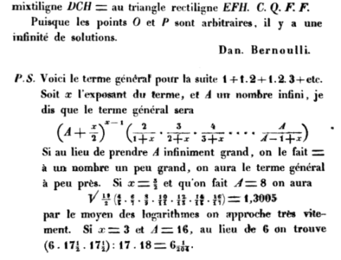
Figure 1.1: Letter from Bernoulli to Goldbach

Part of Bernoulli’s letter [Be29] written 6th October 1729 to Goldbach. It contains the first ever definition of the $\Gamma$-function.

Euler opened his letter with the formula

$$x!=\dfrac{1}{1+x}\left(\dfrac{2}{1}\right)^{x}\cdot\dfrac{2}{2+x}\left(\dfrac{3}{2}\right)^{x}\cdot\dfrac{3}{3+x}\left(\dfrac{4}{3}\right)^{x}\cdot\dfrac{4}{4+x}\left(\dfrac{5}{4}\right)^{x}\cdots$$

but dis also not explain how he arrived at this formula. In fact, a proof had to wait until his 1755 book [E212].

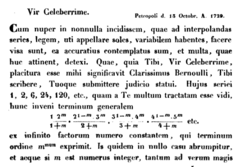
Figure 1.2: Letter from Euler to Goldbach - first Part

First page of Euler’s letter [Eu29] written to Goldbach 13th October 1729 - one week letter than Bernoulli’s. The first page already contains the product representation.

In the same letter, he also said that:

$$m!=\dfrac{1\cdot 2\cdot 3\cdots n}{(1+m)(2+m)(3+m)\cdots(n+m)}(n+1)^{m}$$

for infinite $m$.

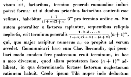
Figure 1.3: Letter from Euler to Goldbach - second Part

Part of the second page of Euler’s letter [Eu29] written to Goldbach 13th October 1729. It already contains what would become known as the Gauß’s product representation of the factorial.

He proved this later in his 1769 paper [E368] and again in his 1793 paper [E652]. Nevertheless, as mentioned, this expression is attributed to Gauß, who used it as a definition for the factorial in his influential 1812 paper [Ga28].
In his letter, concerning his and Bernoulli’s expressions, Euler wrote, translated from the Latin original:
I communicated these discoveries to Bernoulli, who in a peculiar way found almost the same last term, different from mine in that regard that he uses another power instead of $(n+1)^{m}$, determining which he maybe took into account the neglected factors.
This sentence reveals two things: First, Euler knew about Bernoulli’s formula, most probably from private communication. For, the subject was never mentioned in letters they exchanged. Second, he did not know how Bernoulli arrived at his result.
It is speculation, whether Euler found his result influenced by Bernoulli’s formula and, not knowing how the latter arrived at his formula, found his expression or whether he had found it independently. The letter seems to indicate the first option. Dutka in his overview article [Dut91] argues in favour of this possibility, stating the opinion that Bernoulli obtained his formula first and talked to Euler about it and then Euler, after this, found his solution. This is also endorsed by [Gr03]. But one might argue that Euler’s second formula is more natural, since it can be easily found from the recursive property of the factorial and taking the limit. This is also how Euler then proved it in [E652], as we will see below in section 1.4.5. Unfortunately, the question how Bernoulli actually found his formula, remains unsettled. But, having already stated the Bohr-Mollerup theorem above, it is easily checked that also Bernoulli’s expression is another expression for the $\Gamma$-function; $\Gamma(x+1)$, to be precise. Applying the Bohr-Mollerup theorem, we also see that we get another expression for the $\Gamma$-function:

$$\Gamma(x+1)=\lim_{n\rightarrow\infty}A(x,n)^{x-1}\left(\frac{2}{1+x}\cdot\frac{3}{2+x}\cdot\frac{4}{3+x}\cdots\frac{n}{n-1+x}\right)$$

if just $A(x,n)$ is logarithmically convex for $x>1$ and for $n\in\mathbb{N}$ and

$$\lim_{n\rightarrow\infty}A(n,0)\cdot n=1.$$

And Bernoulli’s choice $A(n,x)=\left(n+\frac{x}{2}\right)$ obviously satisfies those requirements. But, e.g., also $\left(n+\frac{x^{k}}{2}\right)^{x-1}$ for a natural number $k$ works as well.
Bernoulli probably preferred his choice, since it converges rapidly to its limit. Thus, the particular choice for $A(n,x)$ is probably a result of extensive calculations trying out several similar formulas.

1.2.3 Overview on Euler’s Contributions

Having now described the history of the $\Gamma$-function in general, we want to give an overview more focused on Euler’s work. To this end, let us first mention that most historical overviews, e.g., [Da59] mostly consider only Euler’s first paper on the $\Gamma-$function [E19] and discuss mainly the two presentations of the $\Gamma$-function Euler gave in that same paper, i.e. his product representation and the integral representation.
But the $\Gamma-$function appears in Euler’s work at several places throughout his career and he devoted several papers to it. Additionally, as we will show below in section 1.5, some of his results he discovered while investigating other subjects can also be applied to the $\Gamma$-function, but Euler did not always do so. To give an example, in his 1750 paper [E123], he considered difference equations of the form:

$$(\alpha x+a)f(x+1)=(\beta x+b)f(x)+(\gamma x+c)f(x-1)$$

but not does not apply it to the functional equation of the $\Gamma-$function, being a special case of the above equation. He did this only in the 1785 paper [E594] on the same subject in section 1.5.2.1. Both papers are actually devoted to continued fractions and the results on the $\Gamma$-function are just a byproduct.
Thus, it will be convenient to give a comprehensive list of Euler’s papers on the $\Gamma$-function and group them into categories, whether they are directly devoted to the $\Gamma$-function or the results are just byproducts of other investigations. Furthermore, in the second part, we want to distinguish, whether Euler realized the consequences from his investigations or not, since on some occasions he did, on others he did not.

1.2.3.1 Euler’s Papers on the $\Gamma$-function

In total, Euler wrote 13 papers either directly devoted to the $\Gamma$-function or containing insights on the $\Gamma-$function as byproducts. The papers devoted to the $\Gamma$-functions are: [E19], [E652], [E661], [E421], [E662], [E816], [E368].
The papers containing results on the $\Gamma$-function as a byproduct are: [E122], [E123], [E189], [E613], [E594], chapter 4, 16 and 17 of the second part of the book [E212].
For the sake of convenience, we want to give a brief summary of each paper and its title already here, although we will mention them in more detail in the corresponding sections. On this occasion, it will be convenient to mention Eneström’s 1910 book [En10], listing all of Euler’s writings in chronological order with a short description of the content. Eneström attributed a number from $1$ to $866$ to each of Euler’s papers or books, referred to a the Eneström number. The smaller the Eneström number is, the earlier the paper was published. We always cite Euler’s papers by their Eneström number.

1. [E19]: De progressionibus transcendentibus seu quarum termini generales algebraice dari nequeunt, published in 1738.
This is Euler’s first paper on the $\Gamma$-function. As mentioned above in section 1.2.1, Euler found the integral representation and the product representation.

2. [E122]: De productis ex infinitis factoribus ortis, published in 1750.
Euler studied $B$-function integrals and derives several relations among them.

3. [E123]: De fractionibus continuis observationes, published in 1750.
This is Euler’s longest paper on continued fractions he ever wrote. It contains many topics, including the transformation of series into continued fractions and the solution of the Riccati differential equation via continued fractions. Additionally, Euler described a method to solve homogeneous difference equations with linear coefficients. See section 1.5.

4. [E189]: De serierum determinatione seu nova methodus inveniendi terminos generales serierum, published in 1753.
Euler solved several difference equations by converting them into a differential equation of infinite order and solving those differential equations then. The factorial is one example he considered. We devote a whole section to the explanation of his ideas. See section 1.6.

5. [E212]: Institutiones calculi differentialis cum eius usu in analysi finitorum ac doctrina serierum, published 1755:
This is Euler’s book on differential calculus. It contains many topics. We mention the introduction of differential quotients, the Euler-Maclaurin summation formula, and many transformation formulas for series as examples. We will mainly focus on his interpolation theory based on difference calculus. See section 1.8.

6. [E368]: De curva hypergeometrica hac aequatione expressa $y=1\cdot 2\cdot 3\cdots x$, published 1769.
This is an overview article on the $\Gamma$-function. Euler stated all formulas he ever found for $x!$ - most of them without out proof -, evaluated the factorial and its derivative for special values.

7. [E421]: Evolutio formulae integralis $\int x^{f-1}dx\left(\log(x)\right)^{\frac{m}{n}}$ integratione a valore $x=0$ ad $x=1$ extensa, published 1772.
This is an overview paper on the integral representation of the $\Gamma$-function. It contains many results - with proofs - e.g., the relation among the $\Gamma$- and $B$-function, the derivation of the sine product formula, even formulas attributed to Gauß. All this will be discussed in LABEL:sec:_Relation_between_Gamma_and_B.

8. [E594]: Methodus inveniendi formulas integrales, quae certis casibus datam inter se teneant rationem, ubi sumul methodus traditur fractiones continuas summandi, published 1785.
This paper can be considered as an addendum to [E123]. It contains several examples not discussed in the latter, including the $\Gamma$-function. Thus, [E594] contains a derivation of the integral representation of the $\Gamma$-function from its functional equation.

9. [E613]: Dilucidationes in capita postrema calculi mei differentalis de functionibus inexplicabilibus, published in 1787.
This is an addendum to chapter 16 and 17 in [E212]. It is a more detailed discussion of his solution of the interpolation problem of a sum using difference calculus. He applied his general formulas to the factorial this time.

10. [E652]: De termino generali serierum hypergeometricarum, published in 1793.
This paper contains the proof of the Gaußian representation of the factorial. The proof is based on the functional equation. We discuss this in 1.4.5.

11. [E661]: Variae considerationes circa series hypergeometricas, published in 1794.
Euler uses the Euler-Maclaurin summation formula to study the factorial.

12. [E662]: De vero valore formulae integralis $\int\partial x\left(\log\frac{1}{x}\right)^{n}$ a termino $x=0$ usque ad terminum $x=1$ extensae, published in 1894, but presented already in 1776.
In this paper, Euler tried to evaluate the integral for several rational numbers. Due to the transcendence of the $\Gamma$-function, his efforts are eventually in vain. Nevertheless, he was able to express products of several values in terms of familiar quantities, like $\pi$ and $\sin\pi x$.

13. [E816]: Considerations sur quelques formules integrales dont les valeurs peuvent etre exprimees, en certains cas, par la quadrature du cercle, published in 1862.
This paper was written in the same spirit as [E662].
Having described all papers briefly, we want to note that the papers [E19], [E368] and [E421] together contain all formulas and insights on the $\Gamma$-function that Euler ever made and had. Thus, we provided a translation of the Latin originals into English of all three papers. They are found in the appendix. As mentioned, the 1738 paper [E19] was the first appearance of the $\Gamma$-function in print ever. The 1772 paper [E421] and the 1769 paper [E368] are rather overview papers. The first is devoted to the integral representation, whereas the second focuses more on the product representations. Thus, they are elaborations on both the representations that appeared already in [E19]. Unfortunately, the proofs of the formulas are not always found in those same papers, but in others. In in some cases, Euler even only gave a heuristic proof.

1.2.3.2 Euler’s Results on the $\Gamma$-function

Here, we want to give a list of Euler’s results on the $\Gamma$-function together with the paper, in which it can be found. How he obtained his result, will be explained below in the corresponding sections in more detail.

1. Integral Representation:
Euler found the function defined as:

$$\int\limits_{0}^{1}\left(\log\dfrac{1}{x}\right)^{n}dx$$

as a solution to the problem of interpolating of the factorial. In [E19] he obtained it rather indirectly from a $B$-function integral. We will see this below in section LABEL:subsubsec:_Using_the_B-function. But confer also [Da59], [Sa07]. The paper [E123], actually devoted to the continued fractions, contains the tools to obtain the integral formula directly. He did this in the paper [E594], also a paper on continued fractions.

2. Euler Product Representation:
By this we mean the formula

$$x!=\dfrac{1}{1+x}\left(\dfrac{2}{1}\right)^{x}\cdot\dfrac{2}{2+x}\left(\dfrac{3}{2}\right)^{x}\cdot\dfrac{3}{3+x}\left(\dfrac{4}{3}\right)^{x}\cdot\dfrac{4}{4+x}\left(\dfrac{5}{4}\right)^{x}\cdots$$

which he first stated without proof in [E19]. It is also stated in the first paragraph of [E368]. But neither of those papers contains a proof. A proof had to wait until 1755 in chapter 16 and 17 of the second part of his book from 1755. There, he solved interpolation problems via difference calculus. The idea is presented in more detail in [E613]. The above formula is just a corollary of more general formulas. Below in section 1.8.4 we will discuss Euler’s ideas from [E613] and show, how they anticipated the fundamental ideas of Weierstraß-products in section LABEL:subsec:_Modern_Idea_-_Weierstrass_product.

3. Gaußian product representation, i.e.

$$x!=\lim_{n\rightarrow\infty}\dfrac{1}{1+x}\cdot\dfrac{2}{2+x}\cdots\dfrac{n}{n+x}(n+1)^{x}.$$

This formula is often attributed to Gauß, since it was the starting point of his investigations on the factorial in the influential paper [Ga28]. But Euler, arguing via infinitely large numbers, proved this formula in [E652]. We will discuss later in section 1.4.5 how he found this product. Additionally, Euler gave this definition in his 1729 letter to Goldbach [Eu29], as we have already seen in section 1.2.2.

4. Stirling formula for $\Gamma(x+1)$:
The Stirling formula says

$$x!=\Gamma(x+1)=\sqrt{2\pi x}\dfrac{x^{x}}{e^{x}}\quad\text{for}\quad x\rightarrow\infty.$$

This formula is attributed to Stirling for his 1730 investigations [St30]. But we will have to say several things concerning priorities below in section 1.6.4.1. Anyhow, Euler proved this formula on two occasions. First, in his 1755 book [E212]. There, the formula is derived as a consequence from his more general results on the Euler-Maclaurin summation formula. We will represent his proof, when discussing the Stirling formula in section 1.6.4.1. [E661] is then solely devoted to investigations of slight generalisations of the factorial functions via the Euler-Maclaurin formula. He also stated the Stirling formula in [E368].
He also tried to give another proof in [E189]. In this paper, he solved difference equations including $f(x+1)-f(x)=\log(x)$, which is solved by $\log\Gamma(x)$ of course, by converting them into differential equations of infinite order first. But his general investigations contain a conceptual error and thus his proof is incorrect. We will elaborate on this below in section 1.6.2.3, discuss his error and give a method how to correct his arguments.

5. Series expansions for $\log\Gamma(x+1)$:
Euler found several series expansions for the logarithm of the $\Gamma-$function, he gave a list in [E368]. Let us mention two striking examples:

$$\log\Gamma(x+1) =-\gamma x+x+\dfrac{1}{2}x+\dfrac{1}{3}x+\dfrac{1}{4}x+\text{etc.}$$

$$-\log\left(1+\dfrac{x}{1}\right)-\log\left(1+\dfrac{x}{2}\right)-\log\left(1+\dfrac{x}{3}\right)-\log\left(1+\dfrac{x}{4}\right)+\text{etc.}$$

Taking the exponentials and applying the functional equation $\Gamma(x+1)=x\Gamma(x)$, we arrive at Newman’s formula which we saw above already

$$\dfrac{1}{\Gamma(z)}=ze^{\gamma z}\left[\left(1+z\right)e^{-z}\right]\left[\left(1+\dfrac{z}{2}\right)e^{-\frac{z}{2}}\right]\cdots.$$

As a second example, we mention the Taylor series expansion of $\log\Gamma(x+1)$:

$$\log\Gamma(x+1)=-\gamma x+\dfrac{\zeta(2)}{2}x^{2}-\dfrac{\zeta(3)}{3}x^{3}+\dfrac{\zeta(4)}{4}x^{4}-\text{etc.}$$

where

$$\zeta(z)=\sum_{k=1}^{\infty}\dfrac{1}{k^{z}}.$$

A proof by Euler can be found in chapter 16 and 17 of the second part of [E212].

6. Reflection formula

$$\dfrac{\pi}{\sin(\pi x)}=\Gamma(x)\Gamma(1-x).$$

He used it in his investigations on the $\zeta$-function in [E352], but provided a proof based on the product formula of the $\Gamma-$function and the sine product formula, discovered in [E41] but proved later in [E61], just in [E421]. Below, in section LABEL:subsubsec:_Euler's_Proof_of_the_Reflection_Formula, we will present this proof and also discuss Euler’s proof of the sine product formula in section LABEL:subsubsec:_Euler's_Proof_of_the_Sine_Product_Formula.

7. Relation among the $\Gamma-$ and $B-$function:

$$B(x,y)=\dfrac{\Gamma(x)\Gamma(y)}{\Gamma(x+y)}.$$

Euler stated this formula on several occasions, e.g. [E421], [E816], [E662]. But he never gave a satisfactory proof.

8. Gaußian multiplication formula:

$$\Gamma\left(\dfrac{x}{n}\right)\Gamma\left(\dfrac{x+1}{n}\right)\cdots\Gamma\left(\dfrac{x+n-1}{n}\right)=\dfrac{(2\pi)^{\frac{n-1}{2}}}{n^{x-\frac{1}{2}}}\cdot\Gamma(x)$$

Euler did not state it in the above form, but, in [E421], he gave the formula:

$$\left[\frac{m}{n}\right]=\frac{m}{n}\sqrt[n]{n^{n-m}\cdot 1\cdot 2\cdot 3\cdots(m-1)\left(\frac{1}{m}\right)\left(\frac{2}{m}\right)\left(\frac{3}{m}\right)\cdots\left(\frac{n-1}{m}\right)}.$$

Here is the explanation of Euler’s notation from [E421]:

$$[x]=x!=\Gamma(x+1)\quad\text{and}\quad\left(\dfrac{p}{q}\right)=\dfrac{1}{n}\int\limits_{0}^{1}dxx^{\frac{p}{n}-1}(1-x)^{\frac{q}{n}-1}=\frac{1}{n}B\left(\frac{p}{n},\frac{q}{n}\right).$$

In section LABEL:subsec:_Multiplication_Formula, we will show that this formula is equivalent to the Gaußian formula. Euler did not prove this formula and only obtains it heuristically by pattern recognition.

9. Expression of $\Gamma\left(\frac{p}{q}\right)$ in terms of integrals of algebraic functions:
In [E19] and [E122], Euler gave the formula

$$\int\limits_{0}^{1}\left(-\log x\right)^{\frac{p}{q}}dx=\sqrt[q]{1\cdot 2\cdot 3\cdots p\left(\dfrac{2p}{q}+1\right)\left(\dfrac{3p}{q}+1\right)\left(\dfrac{4p}{q}+1\right)\cdots\left(\dfrac{qp}{q}+1\right)}$$

$$\times\sqrt[q]{\int\limits_{0}^{1}dx(x-xx)^{\frac{p}{q}}\cdot\int\limits_{0}^{1}dx(x^{2}-x^{3})^{\frac{p}{q}}\cdot\int\limits_{0}^{1}dx(x^{3}-x^{4})^{\frac{p}{q}}\cdot\int\limits_{0}^{1}dx(x^{4}-x^{5})^{\frac{p}{q}}\cdots\int\limits_{0}^{1}dx(x^{q-1}-x^{q})^{\frac{p}{q}}}.$$

1.3 Short modern Introduction to the $\Gamma$-Function

We briefly mention the modern definition of $\Gamma(x)$ following [Fr06] (pp. 194-197). We start from the integral representation and derive the characteristic properties from it. Furthermore, we will obtain two equivalent characterisations of the $\Gamma$-function, based on Wielandt’s theorem in section 1.3.2.1 and the Bohr-Mollerup theorem in section 1.3.2.2.

1.3.1 Definition and simple Properties

1.3.1.1 Definition

Definition 1.3.1 ($\Gamma$-integral).

We define the $\Gamma$-function as a function in the complex plane as the following integral

$$\Gamma(z):=\int\limits_{0}^{\infty}t^{z-1}e^{-t}dt.$$

Here $t^{z-1}:=e^{(z-1)\log(t)}$, $\log t\in\mathbb{R}$, $\operatorname{Re}(z)>0$.

We have the following simple theorem:

Theorem 1.3.1.

The $\Gamma$-integral

$$\Gamma(z):=\int\limits_{0}^{\infty}t^{z-1}e^{-t}dt$$

converges absolutely for $\operatorname{Re}(z)>0$ and represents an analytic function on the domain. The derivatives are given (for $k\in\mathbb{N}$) by

$$\Gamma^{(k)}(z)=\int\limits_{0}^{\infty}t^{z-1}(\log t)^{k}e^{-t}dt.$$

Proof.

We split the $\Gamma$ integral into the two integrals

$$\Gamma(z)=\int\limits_{0}^{1}t^{z-1}e^{-t}dt+\int\limits_{1}^{\infty}t^{z-1}e^{-t}dt$$

and use the relation

$$\left|t^{z-1}e^{-t}\right|=t^{x-1}e^{-t}$$

where we wrote $x$ for $\operatorname{Re}(z)$. Let us consider both integrals separately. In general, for each $x_{0}>0$ there is a number $C>0$ with

$$t^{x-1}\leq Ce^{\frac{t}{2}}\quad\forall\leavevmode\nobreak\ x\quad\text{with}\quad 0<x\leq x_{0}\quad\leavevmode\nobreak\ \text{and}\leavevmode\nobreak\ t\geq 1.$$

Thus, the integral

$$\int\limits_{1}^{\infty}t^{z-1}e^{-t}dt$$

converges absolutely for all $z\in\mathbb{C}$.
For the other integral, we use the estimate

$$\left|t^{z-1}e^{-t}\right|<t^{x-1}\quad\text{for}\leavevmode\nobreak\ t>0$$

and the existence of the integral

$$\int\limits_{0}^{1}\dfrac{1}{t^{s}}dt\quad\text{for}\quad s<1.$$

From these estimates it follows that the sequence of functions

$$f_{n}(z):=\int\limits_{\frac{1}{n}}^{n}t^{z-1}e^{-t}dt$$

converges uniformly to $\Gamma$ for $n\rightarrow\infty$. Therefore, $\Gamma$ is an analytic function.
The formula for the $k-$th derivative follows from the application of the Leibniz rule (for differentiation) and then taking the limit $n\rightarrow\infty.$ ∎

1.3.1.2 Simple Properties

We have

Theorem 1.3.2 (Elementary properties of the $\Gamma$-integral).

The $\Gamma$-function can be analytically continued to the whole complex plane except at the points

$$z\in S:=\{0,-1,-2,-3,\cdots\}$$

and at $\mathbb{C}\setminus S$ satisfies the functional equation:

$$\Gamma(z+1)=z\Gamma(z).$$

All singularities are poles of first order with the residues:

$$\operatorname{Res}(\Gamma,-n)=\dfrac{(-1)^{n}}{n!}$$

Proof.

We show the functional equation first. Obviously, we have

$$\Gamma(1)=\int\limits_{0}^{\infty}e^{-t}dt=\left[-e^{-t}\right]_{0}^{\infty}=1.$$

By integration by parts one arrives at the functional equation

$$\Gamma(z+1)=z\Gamma(z)\quad\text{for}\quad\operatorname{Re}(z)>0.$$

Using the functional equation iteratively, we find

$$\Gamma(z)=\dfrac{\Gamma(z+n+1)}{z\cdot(z+1)\cdots(z+n)}.$$

The right-hand side of the equation has a large domain where it can be defined, i.e.

$$\operatorname{Re}(z)>-(n+1)\quad\text{and}\quad z\neq 0,-1,-2,-3,\cdots,-n.$$

Therefore, the above equation is an analytic continuation of $\Gamma$ into a larger domain.
Finally, let us consider the residues. Using the functional equation, we have

$$\operatorname{Res}(\Gamma;-n)=\lim_{z\rightarrow-n}(z+n)\Gamma(z)=\dfrac{\Gamma(1)}{(-n)(-n+1)\cdots(-1)}=\dfrac{(-1)^{n}}{n!}.$$

∎

1.3.2 Classification Theorems

The $\Gamma$-function was invented by Euler to interpolate the factorial in 1738 [E19]. The integral representation obviously fulfills this task, since $\Gamma(n+1)=n!$. The factorial has these two properties $0!=1$ and $n!=n(n-1)!$. Therefore, this automatically raises the question, whether the $\Gamma$-function is the only holomorphic function with $\Gamma(z+1)=z\Gamma(z)$ and $\Gamma(1)=1$. As already mentioned in section 1.2.1.6, the answer to this question is no, since, e.g.,

$$f(z):=(1+\sin(2\pi z))\Gamma(z)$$

also has these two properties.
Below we will encounter several other expressions also satisfying the functional equation and $f(1)=1$ and above we already did in section 1.2.1.6. Therefore, it will be useful to have theorems that tell us immediately that the new expression is indeed the $\Gamma$-function without showing the equality to the integral representation directly.
This is provided by classification theorems. They state that the $\Gamma$-function can be uniquely defined by the two obvious properties $\Gamma(1)=1$ and $\Gamma(z+1)=z\Gamma(z)$ and an additional third one. We will present two theorems, Wielandt’s theorem and the Bohr-Mollerup theorem. In Bourbaki [Bo51], the Bohr-Mollerup theorem is the starting point for theory of the $\Gamma$-function. There, one does not start from a specific representation.

1.3.2.1 Wielandt’s Theorem

Wielandt’s Theorem is one possible characterisation of the $\Gamma$-function. Wielandt’s original proof can be found in his collected papers [Wi96]. Other proofs can be found, e.g., in the books [Kn41] (pp. 47-49) and [Fr06] (pp. 198-199) which we will present here, and in the paper [Re96].
We have:

Theorem 1.3.3 (Wielandt’s Theorem).

Let $D\subseteq\mathbb{C}$ be a domain containing the vertical strip

$$1\leq x<2.$$

Let $f:D\rightarrow\mathbb{C}$ be a function with the following properties:
1) $f$ is bounded in the vertical strip
2) We have

$$f(z+1)=zf(z)\quad\text{for}\quad z,z+1\in D$$

Then we have:

$$f(z)=f(1)\Gamma(z)\quad\text{for}\quad z\in D.$$

Proof.

Applying the functional equation, it is easily seen that the function $f$ can be analytically continued to the whole complex plane except at the points:

$$z\in S=\{0,-1,-2,-3,\cdots\}$$

and satisfies

$$f(z+1)=zf(z).$$

All $z\in S$ are either poles of first order or removable singularities, and we have:

$$\operatorname{Res}(f;-n)=\dfrac{(-1)^{n}}{n!}f(1).$$

Therefore, the function $h(z):=f(z)-f(1)\Gamma(z)$ is an entire function. Furthermore, it is bounded in the vertical strip $0\leq x\leq 1$, which follows immediately from the boundedness in the strip $1\leq x<2$ and the functional equation for $|\operatorname{Im}(z)|\geq 1$. The domain $|\operatorname{Im}(z)|\leq 1$, $0\leq\operatorname{Re}(z)\leq 1$ is compact.
We want to use Liouville’s theorem and observe that from the functional equation for $h$, i.e. $h(z)z=h(z+1)$, if we define

$$H(z):=h(z)h(1-z),$$

we find $H(z+1)=-H(z)$. But the strip $0\leq x\leq 1$ is not changed under the transformation $z\rightarrow 1-z$. Thus, $H$ is bounded on this strip and, because of the periodicity, it is bounded on $\mathbb{C}$. Therefore, Liouville’s theorem implies that $H$ is constant. But $h(1)=0$, so $H=0$ and hence also $h=0$ for all $z\in\mathbb{C}$. ∎

The $\Gamma$-integral obviously satisfies all three properties. We will see this below, when we find the integral representation from the moment ansatz in section 1.5.

1.3.2.2 Bohr-Mollerup Theorem

The Bohr-Mollerup Theorem, first proved in the 1922 book [Mo22], also states that the Gamma function can be uniquely classified by three properties. In other words, aside from the two obvious ones $\Gamma(x+1)=x\Gamma(x)$, $\Gamma(1)=1$, we, as in the case of Wielandt’s theorem, need one additional property. This is the so-called logarithmic convexity. For the sake of completeness, let us define convexity first and show that $\Gamma(x)$ has the property of logarithmic convexity, before we get to the theorem.

Definition 1.3.2 (Logarithmic Convexity).

Let $X,Y$ be open subsets of the real numbers $\mathbb{R}$. Further, let $f:X\rightarrow Y$ be a function. Then, $f$ is called convex, if the following inequality holds:

$$f(tx+(1-t)y)\leq tf(x)+(1-t)f(y)\quad\forall\leavevmode\nobreak\ x,y\in X,\quad\forall t\in\left[0,1\right]$$

Furthermore, $f$ is called logarithmically convex , if $\log f(x)$ is convex.

Let us state a theorem which can be used if $f$ additionally is twice continuously differentiable.

Theorem 1.3.4.

If the second derivative of a twice continuously differentiable function is always $\geq 0$ in the interval $(a,b)$, then the function $f$ is convex in this interval. The converse of this theorem is also true.

The proof can be found in every book on analysis of one variable, one can also find a proof in [Ar15] (pp. 6-7). We will need the following corollary.

Corollary 1.3.4.1.

If $f:\mathbb{R}\rightarrow\mathbb{R}$ is twice continuously differentiable and the following inequalities are satisfied for all $x\in(a,b)$

$$f(x)>0,\quad f(x)f^{\prime\prime}(x)-(f^{\prime}(x))^{2}\geq 0,$$

then $\log f$ is convex, i.e. $f$ is logarithmically convex, in this interval.

For a proof one just has to apply the previous theorem to $\log f$. Further, we have

Corollary 1.3.4.2.

The sum of two logarithmically convex function is also logarithmically convex.

We will not prove this statement here. For a proof the reader is referred to [Ar15]. Instead, we want to go over to the logarithmic convexity of $\Gamma$. For this, consider $f(t,x)$, continuous in both variables $x$ and $t$. Let $a\leq t\leq b$ and $x$ live in another interval. If $f(t,x)$ now is logarithmically convex for all $t$ and twice continuously differentiable with respect to $x$, define:

$$F_{n}(x)=h\left\{f(a,x)+f(a+h,x)+f(a+2h,x)+\cdots+f(a+(n-1)h,x),\quad h=\dfrac{b-a}{n}\right\}$$

Then, $F_{n}(x)$ is also logarithmically convex for all $n\in\mathbb{N}$. Therefore, also

$$\lim_{n\rightarrow\infty}F_{n}(x)=\int\limits_{a}^{b}f(t,x)dt$$

is logarithmically convex. This also holds for improper integrals, if the integral exists. Therefore, we have:

Theorem 1.3.5.

The $\Gamma$- function, given as

$$\int\limits_{0}^{\infty}t^{x-1}e^{-t}dt,$$

is logarithmically convex for $x>0$.

Now, having mentioned all this in advance, we can finally state the Bohr-Mollerup theorem.

Theorem 1.3.6 (Bohr-Mollerup Theorem).

If a function $f:\mathbb{R}^{+}\rightarrow\mathbb{R}$ satisfies the three properties
1) $f(x+1)=xf(x)$
2) $f$ is logarithmically convex on the whole domain where it is defined
3) $f(1)=1$,
it is identical to the $\Gamma$-function in the region where it is defined.

Proof.

We have shown that $\Gamma$ satisfies all conditions. Therefore, let $f$ be another function with the above properties. From the functional equation we find

$$f(x+n)=(x+n-1)(x+n-2)\cdots(x+1)xf(x).$$

Since $f(1)=1$ we have $f(n)=\Gamma(n)\leavevmode\nobreak\ \forall n\in\mathbb{N}$. We only need to show $f=\Gamma$ for the interval $0<x\leq 1$, because of the functional equation. Thus, let $x$ be a number in that interval and $n$ a natural number $\geq 2$. Then, we have the following inequality

$$\dfrac{\log(f(-1+n))-\log(f(n))}{(-1+n)-n}\leq\dfrac{\log(f(x+n))-\log(f(n))}{(x+n)-n}\leq\dfrac{\log(f(1+n))-\log(f(n))}{(1+n)-n}$$

which follows from the logarithmic convexity. We can simplify the last equation:

$$\log(n-1)\leq\dfrac{\log(f(x+n))-\log(f(n))}{(x+n)-n}\leq\log n$$

or

$$\log((n-1)^{x}(n-1)!)\leq f(x+n)\leq\log(n^{x}(n-1)!).$$

Using the above equation for $f(x+n)$:

$$\dfrac{(n-1)^{x}(n-1)!}{x(x+1)\cdots(x+n-1)}\leq f(x)\leq\dfrac{n^{x}(n-1)!}{x(x+1)\cdots(x+n-1)}=\dfrac{n^{x}n!}{x(x+1)\cdots(x+n)}\cdot\dfrac{x+n}{n}.$$

Since we assumed $n\geq 2$, we can replace $n$ by $n+1$ and find:

$$\dfrac{n^{x}n!}{x(x+1)\cdots(x+n)}\leq f(x)\leq\dfrac{n^{x}n!}{x(x+1)\cdots(x+n)}\cdot\dfrac{x+n}{n}.$$

Therefore,

$$f(x)\dfrac{n}{n+x}\leq\dfrac{n^{x}n!}{x(x+1)\cdots(x+n)}\leq f(x).$$

Taking the limit $n\rightarrow\infty$:

$$f(x)=\lim_{n\rightarrow\infty}\dfrac{n^{x}n!}{x(x+1)\cdots(x+n)}.$$

Since the function $f$ only had to satisfy the three conditions in the theorem and was arbitrary otherwise, we conclude $f(x)=\Gamma(x)$. ∎

We have the following corollary:

Corollary 1.3.6.1.

$$\Gamma(x)=\lim_{n\rightarrow\infty}\dfrac{n^{x}n!}{x(x+1)\cdots(x+n)}.$$

We will find other ways to get to this product representation below. It is interesting that it follows directly from the proof. Additionally, we already pointed out in section 1.2.1.2 that Gauß in 1812 [Ga28] used the last corollary as a definition for the $\Gamma$-function. However, we already saw in section 1.2.2 that this product formula had already been discovered by Euler in [Eu29].

1.4 Solution of the Difference Equation $F(x+1)=xF(x)$

In this section we will solve the functional equation in general and from there descend to the $\Gamma$-function. This will lead us to the Weierstraß product expansion of the $\Gamma$-function. Our exposition follows [Ni05].

1.4.1 Weierstraß’s Definition of the $\Gamma$-function

It was Weierstraß’s [We56] idea to define the $\Gamma$-function as solution of the difference equation

$$F(x+1)=xF(x)$$

with the additional condition

$$\lim_{n\rightarrow\infty}\dfrac{F(x+n)}{(n-1)!n^{x}}=1.$$

The above condition, as we will see soon, excludes solutions of the form $\Gamma(x)p(x)$ with $p$ a periodic function with period $1$.
Anyhow, in this section we want to solve the difference equation in general and want to show that it indeed defines the $\Gamma$-function as claimed.

1.4.2 A Remark concerning the Solution of the Difference Equation

Let us begin with the following remark:

Remark 1.

In order to solve the difference equation $F(x+1)=xF(x)$, we essentially only need one particular solution.

Proof.

For, let $F_{1}(x)$ and $F_{2}(x)$ be two particular solutions of the difference equation. Then, one has

$$\dfrac{F_{2}(x+1)}{F_{1}(x+1)}=\dfrac{xF_{2}(x)}{xF_{1}(x)}=\dfrac{F_{2}(x)}{F_{1}(x)},$$

i.e. the quotient of the two solutions is a periodic function with period $+1$. In other words, if $F_{1}(x)$ is a solution of the difference equation, then every other solution $F_{2}(x)$ is connected to it by

$$F_{2}(x)=\omega(x)F_{1}(x)\quad\text{with}\quad\omega(x+1)=\omega(x).$$

∎

1.4.3 General Solution of the Equation $F(x+1)=xF(x)$

1.4.3.1 Introduction of an Auxiliary Function

Keeping the remark of the previous section in mind, we can now proceed to find a solution of the difference equation and show that the $\Gamma$-function is actually the only one. For this aim, let us introduce the following function:

Definition 1.4.1.

We define a function $\Sigma:\mathbb{C}\setminus\{0,-1,-2,-3,\cdots\}\rightarrow\mathbb{C}$ by the sum

$$\Sigma(x):=\sum_{s=0}^{\infty}\left(\dfrac{1}{s+1}-\dfrac{1}{x+s}\right).$$

This series is easily seen to converge uniformly. Thus, we are allowed to integrate it term by term with respect to $x$, provided the path of integration is of finite length and does not pass through any of the poles.
Furthermore, we have

Theorem 1.4.1.

$\Sigma$ satisfies the functional equation

$$\Sigma(x+1)=\Sigma(x)+\dfrac{1}{x}.$$

Proof.

Consider the difference $\Sigma(x+1)-\Sigma(x)$; it reads

$$\begin{array}[]{llllll}&\sum_{s=0}^{\infty}\left(\dfrac{1}{s+1}-\dfrac{1}{x+1+s}\right)-\sum_{s=0}^{\infty}\left(\dfrac{1}{s+1}-\dfrac{1}{x+s}\right)\\ \leavevmode\nobreak\ =\nobreak\leavevmode&\sum_{s=0}^{\infty}\left(\dfrac{1}{s+1}-\dfrac{1}{x+1+s}\right)-(1-\dfrac{1}{x})-\sum_{s=0}^{\infty}\left(\dfrac{1}{s+2}-\dfrac{1}{x+1+s}\right)\\ \leavevmode\nobreak\ =\nobreak\leavevmode&1-1+\dfrac{1}{x}=\dfrac{1}{x},\end{array}$$

since the sums involving $x$ cancel and the sums involving only $s$ are telescoping sums. ∎

1.4.3.2 Product Representation of the Function $F$

Theorem 1.4.2.

Every meromorphic function $F$ satisfying the equation $F(x+1)=xF(x)$ has a product expansion of the form

$$F(x+1)=\omega(x)\cdot\dfrac{e^{Kx}}{x}\cdot\prod_{s=1}^{\infty}\dfrac{e^{\frac{x}{s}}}{1+\frac{x}{s}},$$

where $K$ is a constant and $\omega:\mathbb{C}\rightarrow\mathbb{C}$ is a integrable and periodic function with period $+1$.

Proof.

Let $\omega(x)$ be as above, and let it be integrable on $(0,x)$ with $x>0$. Define

$$\omega_{1}(x):=\int\limits_{0}^{x}\omega(x)dx.$$

Then $\omega_{1}(x)$ satisfies the functional equation:

$$\omega_{1}(x+1)=\omega_{1}(x)+K,$$

$K$ being a constant. Now, recalling the definition of the function $\Sigma$ from section 1.4.3.1, by integration we find

$$\log F(x+1)=\int\limits_{0}^{x}\Sigma(x+1)dx+K\cdot(x+1)$$

or, equivalently substituting the series for $\Sigma$ and integrating it term by term, we have

$$\log F(x+1)=\sum_{s=0}^{\infty}\left(\dfrac{x}{s+1}-\log\left(1+\dfrac{x}{s+1}\right)\right)+K\cdot(x+1).$$

Thus, taking the exponentials, we find

$$F(x)=\omega(x)\cdot\dfrac{e^{Kx}}{x}\cdot\prod_{s=1}^{\infty}\dfrac{e^{\frac{x}{s}}}{1+\frac{x}{s}}.$$

∎

Thus, to summarize the proof: We basically solved the simpler equation $f(x+1)-f(x)=\frac{1}{x}$ first. A particular solution is given by our function $\Sigma$. Thus, by integrating, we can then deduce the solution of $g(x+1)-g(x)=\log(x)$ and by taking the exponentials we arrive at the functional equation for $F(x)$. It is helpful to keep this in mind, since this is also basically what Euler did in 1780 in [E613] and in 1755 in [E212] to find the product representation of the $\Gamma$-function. In other words, this proof can easily be constructed from Euler’s ideas in that paper.

1.4.3.3 Finding the Constant $K$

Finally, we need to find the constant $K$, which was introduced by an integration in the previous section. Hence let us introduce the sequence of functions $G_{n}:\mathbb{C}\setminus\{{0,-1,-2,\cdots-(n-1)\}}\rightarrow\mathbb{C}$ defined by

$$G_{n}(x):=\dfrac{e^{Kx}}{x}\prod_{s=1}^{n-1}\dfrac{e^{\frac{x}{s}}}{1+\frac{x}{s}}.$$

From this

$$G_{n}(x+1)=\dfrac{e^{Kx}\cdot e^{K}}{x+1}\cdot\prod_{s=1}^{n-1}\dfrac{e^{\frac{x}{s}}\cdot e^{\frac{1}{s}}}{1+\frac{x}{s+1}}\cdot\dfrac{s}{s+1}$$

We want to rewrite this as

$$G_{n}(x+1)=\dfrac{e^{Kx}\cdot e^{K}}{x+1}\cdot\prod_{s=1}^{n-1}\dfrac{e^{\frac{x}{s}}}{1+\frac{x}{s+1}}\cdot e^{\frac{1}{s}-\log\left(1+\frac{1}{s}\right)}.$$

Now using the well-known result that

$$\lim_{n\rightarrow\infty}\sum_{s=1}^{n-1}\left(\frac{1}{s}-\log\left(1+\frac{1}{s}\right)\right)=\gamma$$

where $\gamma$ is the Euler-Mascheroni constant, we know that the limit exists. Define

$$\gamma_{n}=\dfrac{1}{1}+\dfrac{1}{2}+\cdots+\dfrac{1}{n}-\log n$$

such that also $\gamma=\lim_{n\rightarrow\infty}\gamma_{n}$. Then, we have

$$G_{n}(x)=\dfrac{e^{-\gamma_{n}x+\frac{x}{n}}}{x}\prod_{s=1}^{n-1}\dfrac{e^{\frac{x}{s}}}{1+\frac{x}{1+\frac{x}{s}}}$$

and the functional equation

$$G_{n}(x+1)=x\cdot G_{n}(x)\cdot\dfrac{n}{n+x}.$$

Therefore, we have:

Theorem 1.4.3.

Let $\gamma$ be the Euler-Mascheroni constant. Further, let $\omega:\mathbb{C}\rightarrow\mathbb{C}$ be an arbitrary function satisfying $\omega(x+1)=\omega(x)$; then, the most general solution of the difference equation $F(x+1)=xF(x)$ is given by

$$F(x)=\omega(x)\cdot\dfrac{e^{-\gamma x}}{x}\cdot\prod_{s=1}^{\infty}\dfrac{e^{\frac{x}{s}}}{1+\frac{x}{s}}.$$

1.4.4 Application to $\Gamma(x)$- The Weierstraß Product Representation

Now that we found the most general solution of the difference equation $F(x+1)=xF(x)$, we want to descend to $\Gamma(x)$ from this. This is, e.g., possible by an application of the Bohr-Mollerup theorem.
Doing so, we will arrive at the following theorem

Theorem 1.4.4 (Weierstraß Product Expansion of $\Gamma(x)$).

The $\Gamma$-function has the following product expansion:

$$\Gamma(x)=\dfrac{e^{-\gamma x}}{x}\cdot\prod_{s=1}^{\infty}\dfrac{e^{\frac{x}{s}}}{1+\frac{x}{s}}.$$

Proof.

We need to check whether the three conditions in the Bohr-Mollerup theorem are fulfilled. Therefore, let us check $\Gamma(1)=1$ first.
We have

$$\Gamma(1)=e^{-\gamma}\cdot\prod_{s=1}^{\infty}\dfrac{e^{\frac{1}{s}}}{1+\frac{1}{s}}$$

or, by taking logarithms,

$$\log\Gamma(1)=-\gamma+\sum_{s+1}^{\infty}\left(\dfrac{1}{s}-\log\left(1+\dfrac{1}{s}\right)\right)$$

But, as we have seen above, the sum evaluates to $\gamma$, whence $\log\Gamma(1)=1$ or $\Gamma(1)=1$. Hence the first condition is satisfied.
The second condition of the Bohr-Mollerup Theorem, i.e. $\Gamma(x+1)=x\Gamma(x)$ is satisfied, since it solves the general difference equation $F(x+1)=xF(x)$.
Finally, let us check logarithmic convexity. Obviously, $\log\Gamma(x)$ is twice continuously differentiable, since the resulting sum converges uniformly. We find

$$\dfrac{d}{dx}\log\Gamma(x)=-\gamma-\dfrac{1}{x}+\sum_{s=1}^{\infty}\left(\dfrac{1}{s}-\dfrac{1}{1+\frac{x}{s}}\cdot\frac{1}{s}\right)$$

and

$$\dfrac{d^{2}}{dx^{2}}\log\Gamma(x)=\dfrac{1}{x^{2}}+\sum_{s=1}^{\infty}\dfrac{1}{s^{2}}\cdot\dfrac{1}{(1+\frac{x}{s})^{2}},$$

Therefore, obviously $\dfrac{d^{2}}{dx^{2}}\log\Gamma(x)>0\leavevmode\nobreak\ \forall x>0$.
Hence the Bohr-Mollerup theorem applies and the function defined by the infinite product is indeed the familiar $\Gamma$-function. ∎

1.4.5 Euler on Weierstraß’s Condition

We want to show how Euler already arrived at the condition for the $\Gamma$-function that Weierstraß used to introduce it. Note that since we obtained that, if in the above theorem, we chose the periodic function $\omega(x)$ to be $=1$, $F(x)=\Gamma(x)$, we proved that:

Theorem 1.4.5.

The $\Gamma$-function can also be defined by Weierstraß’s conditions, i.e. the $\Gamma$ function is the unique meromorphic function satisfying

$$\Gamma(x+1)=x\Gamma(x)$$

and

$$\lim_{n\rightarrow\infty}\dfrac{\Gamma(x+n)}{(n-1)!n^{x}}=1.\quad\forall\leavevmode\nobreak\ x\in\mathbf{C}\setminus\left\{0,-1,-2,-3,\cdots\right\}$$

We will present how Euler obtained this condition in [E652]. Weierstraß in 1856 in [We56] attributed it to Gauß who introduced this condition in [Ga28].
We will show it for $\Gamma(x+1)$, since in 1793 paper [E652] Euler also did it for $x!$. Euler’s idea was to consider $n$ as a very large natural number and $x$ as a fixed finite natural number with $x\ll n$ and evaluate $\Gamma(x+n+1)$ in two ways. Using the functional equation $x$ times, we have

$$\Gamma(x+1+n)=(x+n)(x+n-1)\cdots(n+1)\Gamma(n+1).$$

But, since $x\ll n$, the finite parts added to $n$ in each factor can be ignored such that

$$\Gamma(x+1+n)\approx n^{x}\Gamma(n+1).$$

On the other hand, we can use the functional equation $n$ times, to find:

$$\Gamma(x+n+1)=(n+x)(n+x-1)\cdots(x+1)\Gamma(x+1).$$

Therefore, dividing both expressions expressions for $\Gamma(x+n+1)$, using $\Gamma(n+1)=n!$ and solving for $\Gamma(x+1)$, we arrive at the formula:

$$\Gamma(x+1)\approx\dfrac{n^{x}n!}{(x+1)\cdots(n+x-1)(n+x)}\quad\text{for}\quad x\ll n.$$

In modern notation, this is the condition in the theorem. One just has to use the functional equation on $\Gamma(x+n)$ $n$ times to arrive at Euler’s and Gauß’s formula. Note that although the proof required $x$ and $n$ to be natural numbers, the right-hand side does not require $x$ to be a natural number. Therefore, it can also be used to interpolate $x!=\Gamma(x+1)$. Additionally, we point out again that Gauß [Ga28] used this formula to introduce the $\Gamma$-function, but he did not motivate it at all.
Euler’s reasoning, using infinitely large numbers, is obviously not rigorous enough for modern times. But, in possession of the Bohr-Mollerup theorem, one could start from this expression and check, whether all conditions are satisfied or not. But since we already did it for the Weierstraß product and know this expression to be equivalent to it, we do not want to repeat this here.

1.5 Euler’s direct Solution of the Equation $\Gamma(x+1)=x\Gamma(x)$ - The Moment Ansatz

We now go over to Euler’s different approaches leading him to an explicit formula of the $\Gamma$-function. We will start with the "moment ansatz", a name that will become clear later. First, we want to explain briefly, where the method actually originated.

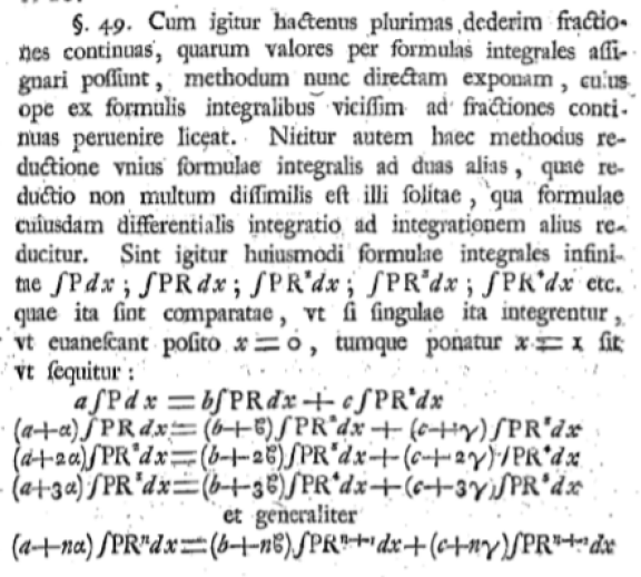
Figure 1.4: Moment Method

One page of Euler’s paper [E123]. Euler explains his idea how to solve the difference equation $(a+\alpha x)f(x)=(b+\beta x)f(x+1)+(c+\gamma x)f(x+2)$ by assuming it to be a certain integral ($\S$ 49). In the following paragraphs he applies it to continued fractions, which was his actual intention in that paper.

1.5.1 Origin of the Idea

Euler uses a technique, which we will refer here to as moment ansatz, to solve difference equations of the kind:

$$(a+\alpha x)f(x)=(b+\beta x)f(x+1)+(c+\gamma x)f(x+2),$$

where $\alpha,\beta,\gamma\leavevmode\nobreak\ \in\mathbb{R}\setminus\{0\}$ and $a,b,c\leavevmode\nobreak\ \in\mathbb{R}$, in his papers [E123] and [E594]. His actual intention was to derive continued fractions from this. For, dividing the above equation by $(a+\alpha x)$ and $f(x+1)$, one will find

$$\dfrac{f(x)}{f(x+1)}=\dfrac{b+\beta x}{a+\alpha x}+\dfrac{c+\gamma x}{a+\alpha x}\dfrac{f(x+2)}{f(x+1)}$$

or

$$\dfrac{f(x)}{f(x+1)}=\dfrac{b+\beta x}{a+\alpha x}+\dfrac{c+\gamma x}{a+\alpha x}\dfrac{1}{\frac{f(x+1)}{f(x+2)}}.$$

Replacing $x$ by $x+1$ one will get a similar equation for the quotient $\frac{f(x+1)}{f(x+2)}$ which can be inserted in the above equation. Repeating this procedure infinitely often, one will get a continued fraction for $\frac{f(x)}{f(x+1)}$.
Euler was interested in the continued fraction arising from this and he tried to solve the difference equation. In the following, we will explain how he did this.

$$A(x)f(x)=B(x)f(x+1)+C(x)f(x+2)$$

with more general functions $A(x)$, $B(x)$, $C(x)$ etc. also leads to continued fractions. But Euler only considered the case in which those functions are linear functions in his papers [E123] and [E594]. Indeed, his investigations do not go beyond the case of linear functions in any of his papers.

1.5.2 Euler’s Idea

Let us discuss his idea on the concrete example of the above difference equation. The generalisation to the general difference equation with linear coefficients is immediate. Euler assumed that the solution is given as an integral of the form

$$\int\limits_{a}^{b}t^{x-1}P(t)dt,$$

whence we have to determine the limits of the integration and the function $P(t)$. Euler, in modern formulation, assumed the solution of the difference equation to be the $x$-th moment of the function $P$. This is why we gave the method the name moment ansatz. In order to do so, Euler considered the auxiliary equation

$$(a+\alpha x)\int\limits^{t}t^{x-1}P(t)dt=(b+\beta x)\int\limits^{t}t^{x}P(t)dt+(c+\gamma x)\int\limits^{t}t^{x+1}P(t)dt+t^{x}Q(t);$$

here, $\int\limits^{t}$ is supposed to denote the indefinite integral over $t$ and $Q(t)$ is another function we have to determine; the use of this function will become clear in a moment.
Euler then differentiated the auxiliary equation with respect to $t$:

$$(a+\alpha x)t^{x-1}P(t)=(b+\beta x)t^{x}P(t)+(c+\gamma x)t^{x+1}P(t)+xt^{x-1}Q(t)+t^{x}Q^{\prime}(t).$$

Now divide by $t^{x-1}$:

$$(a+\alpha x)P(t)=(b+\beta x)tP(t)+(c+\gamma x)t^{2}P(t)+xQ(t)+tQ^{\prime}(t).$$

Comparing the coefficients of the powers of $x$, we will get the following systems of coupled equations:

$$\begin{array}[]{llllllll}1.&aP(t)&\leavevmode\nobreak\ =\nobreak\leavevmode&btP(t)&\leavevmode\nobreak\ +\nobreak\leavevmode&ct^{2}P(t)&\leavevmode\nobreak\ +\nobreak\leavevmode&tQ^{\prime}(t)\\ 2.&\alpha P(t)&\leavevmode\nobreak\ =\nobreak\leavevmode&\beta tP(t)&\leavevmode\nobreak\ +\nobreak\leavevmode&\gamma t^{2}P(t)&\leavevmode\nobreak\ +\nobreak\leavevmode&Q(t)\end{array}$$

Solving both equations for $P$, we find

$$\begin{array}[]{llllllll}1.&P(t)&\leavevmode\nobreak\ =\nobreak\leavevmode&\dfrac{tQ^{\prime}(t)}{a-bt-ct^{2}}\\ 2.&P(t)&\leavevmode\nobreak\ =\nobreak\leavevmode&\dfrac{Q(t)}{\alpha-\beta t-\gamma t^{2}}\end{array}$$

Therefore, we obtain the following equation for $Q(t)$

$$\dfrac{tQ^{\prime}(t)}{Q(t)}=\dfrac{a-bt-ct^{2}}{\alpha-\beta t-\gamma t^{2}}$$

Although this equation can be solved in general, we will not do this here, because it will be more illustrative to consider examples. Anyhow, having found $Q(t)$, we can also find $P(t)$ substituting the value of $Q(t)$ in one of the above equations.
Finally, we need the term $t^{x}Q(t)$ to vanish in the auxiliary equation. Hence the limits of integration are found from the solutions of the equation $t^{x}Q(t)=0$.

1.5.2.1 Application to the $\Gamma$-function - Finding the Integral Representation

As mentioned, everything becomes a lot clearer in certain examples. Therefore, let us consider the $\Gamma$-function, i.e. the functional equation $f(x+1)=xf(x)$. Euler considered the factorial explicitly in $\S 13$ of [E594], a paper published in 1785. We make the ansatz

$$f(x)=\int\limits_{a}^{b}t^{x-1}P(t)dt.$$

Hence we need to determine $P(t)$ and the limits of integration $a$ and $b$. Let us introduce the auxiliary equation:

$$\int\limits^{t}t^{x}P(t)dt=x\int\limits^{t}t^{x-1}P(t)dt+t^{x}Q(t)$$

Differentiating with respect to $t$ gives

$$t^{x}P(t)=xt^{x-1}P(t)+xt^{x-1}Q(t)+t^{x}Q^{\prime}(t).$$

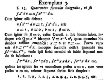
Figure 1.5: Euler finds the Integral Representation of $\Gamma(x)$ via the Moment Method

This is one of the examples that Euler considered. It led him to the familiar integral representation of the the $\Gamma$-function. Euler called the sequence of the factorial "hypergeometric series". The scan is taken from [E594].

Division by $t^{x-1}$ gives

$$tP(t)=xP(t)+xQ(t)+tQ^{\prime}(t).$$

Therefore, comparing the coefficients of $x$:

$$\begin{array}[]{lrlllll}1.&tP(t)&\leavevmode\nobreak\ =\nobreak\leavevmode&tQ^{\prime}(t)\\ 2.&0&\leavevmode\nobreak\ =\nobreak\leavevmode&P(t)+Q(t).\end{array}$$

Solving both equations for $P(t)$:

$$\begin{array}[]{llllllll}1.&P(t)&\leavevmode\nobreak\ =\nobreak\leavevmode&Q^{\prime}(t)\\ 2.&P(t)&\leavevmode\nobreak\ =\nobreak\leavevmode&-Q(t).\end{array}$$

Hence we obtain the following differential equation for $Q(t)$:

$$\dfrac{Q^{\prime}(t)}{Q(t)}=-1.$$

This equation is easily integrated and gives

$$\log(Q(t))=C-t\quad\text{or}\quad Q(t)=Ce^{-t},$$

where $C\neq 0$ is an arbitrary constant of integration. From this $P$ is found to be

$$P(t)=-e^{-t}.$$

Finally, we need to find the limits of integration. For this, we consider the equation $t^{x}Q(t)=Ct^{x}e^{-t}=0$. For $x>0$ we find the two solution $t=0$ and $t=\infty$. Therefore, the term $t^{x}Q(t)$ in the auxiliary equation vanishes in these cases and we find:

$$C\int\limits_{0}^{\infty}t^{x}e^{-t}dt=xC\int\limits_{0}^{\infty}t^{x-1}e^{-t}dt.$$

In other words, the equation $f(x+1)=xf(x)$ is satisfied by:

$$f(x)=C\int\limits_{0}^{\infty}t^{x-1}e^{-t}dt.$$

This is, of course, almost the famous integral representation of the $\Gamma$-function. (There the constant $C$ is one.)

Finding the Integral Representation of $\Gamma(x)$

We can force the function $f$ to be the $\Gamma$ by demanding it to satisfy all conditions of Wielandt’s theorem. The condition $\Gamma(1)=1$ forces $C=1$. More precisely, we have the theorem:

Theorem 1.5.1 (Integral Representation of $\Gamma(x)$).

The $\Gamma$-function is given by the following integral:

$$\Gamma(x)=\int_{0}^{\infty}t^{x-1}e^{-t}dt\quad\text{for}\quad\operatorname{Re}x>0.$$

Proof.

We have to check all conditions of Wielandt’s theorem. First, find $\Gamma(1)$.

$$\Gamma(1)=\int_{0}^{\infty}e^{-t}dt=\left[-e^{t}\right]_{0}^{\infty}=0-(-1)=1.$$

Secondly, the functional equation is satisfied, as demonstrated in the last section.
Finally, we have to check holomorphy (which is obvious) and that $\Gamma(x)$ is bounded in the strip $S:=\{x|1\leq x<2\}$. Hence consider

$$|\Gamma(x)|=\left|\int_{0}^{\infty}t^{x-1}e^{-t}dt\right|\leq\int_{0}^{\infty}\left|t^{x-1}\right|e^{-t}dt$$

In other words, we have

$$|\Gamma(x)|\leq\operatorname{Re}(\Gamma(x))\quad\text{for}\quad\operatorname{Re}x>0.$$

For checking Wielandt’s theorem we have to consider

$$\int_{0}^{\infty}t^{x-1}e^{-t}dt\quad\text{for}\quad 1\leq x<2.$$

But these integrals are obviously bounded, whence Wieldlandt’s theorem applies. ∎

1.5.2.2 Some Remarks on the Ansatz

We assume the solution to have the form $\int t^{x-1}P(t)dt$, which explains the name moment ansatz. But one can, of course, make other choices for the integrand. For the sake of an example, one can set $\int(R(t))^{x-1}$. By the same procedure, one would then arrive at the equation

$$\Gamma(x)=\int\limits_{0}^{1}\left(\log\dfrac{1}{t}\right)^{x-1}dt.$$

This was Euler’s preferred integral representation and actually the first he found in 1738 in [E19]. It follows from the representation just found by setting $e^{-t}=u$.
Furthermore, one can even generalize the ansatz to

$$f(x)=\int R(t)^{x-1}P(t)dt,$$

where $R(t)$ is another function to be determined. Carrying out the procedure as above, one would arrive at certain conditions on the function $R(t)$ which are trivially satisfied by $R(t)=t$. Indeed, Euler tried this most general ansatz in his 1750 paper [E123], but realizing that $R(t)=t$ meets all requirements, he quickly focused on that special case.

1.5.3 Examples of other Equations which can be solved by this Method

Having found the integral representation of the $\Gamma$-function from its difference equation, let us apply Euler’s method to more complicated but still familiar difference equations in order to find some interesting integral representations.

1.5.3.1 1. Example: Legendre Polynomials

The Legendre polynomials satisfy the following difference equation

$$(n+1)P_{n+1}(x)=(2n+1)xP_{n}(x)-nP_{n-1}(x).$$

Together with the conditions $P_{0}(x)=1$ and $P_{1}(x)=x$, this difference equation determines them completely. The moment ansatz can be used to find an explicit formula for $P_{n}(x)$. More precisely, we have the theorem:

Theorem 1.5.2 (Integral representation for the $n$-th Legendre Polynomial).

We have

$$P_{n}(x)=\dfrac{1}{\log(-1)}\int\limits_{x-\sqrt{x^{2}-1}}^{x+\sqrt{x^{2}-1}}\dfrac{t^{n}}{\sqrt{1-2xt+t^{2}}}dt.$$

where the principal branch of $\log(-1)$ is to be taken.

Proof.

This expression can be found by the moment ansatz. Since this is our first concrete example of a second order difference equation and one has to be more careful than in the case of the $\Gamma$-function, let us present the calculation in detail. We start with the auxiliary equation again which reads

$$(n+1)\int\limits^{t}t^{n}R(x,t)dt=(2n+1)x\int\limits^{t}t^{n-1}R(x,t)dt-n\int\limits^{t}t^{n-2}R(x,t)dt+Q(x,t)t^{n}.$$

We wish to find $R(x,t)$ and $Q(x,t)$ and the limits of integration. Let us differentiate that equation with respect to $t$, we find:

$$(n+1)t^{n}R(x,t)=(2n+1)xt^{n-1}R(x,t)-nt^{n-2}R(x,t)+{Q^{\prime}}(x,t)t^{n}+nt^{n-1}Q(x,t).$$

Dividing by $t^{n-2}$ and comparing the coefficients of the powers of $n$, we obtain the following system of equations

$$\begin{array}[]{lll}1.\quad t^{2}R(x,t)&=&2tR(x,t)x-R(x,t)+tQ(x,t)\\ 2.\quad t^{2}R(x,t)&=&tR(x,t)x+Q^{\prime}(x,t)t^{2}\end{array}$$

Solving both for $R(x,t)$

$$\begin{array}[]{lll}1.\quad R(x,t)&=&\dfrac{tQ(x,t)}{t^{2}-2tx+1}\\ 2.\quad R(x,t)&=&\dfrac{t^{2}{Q^{\prime}}(x,t)}{t^{2}-xt}\end{array}$$

Therefore,

$$\dfrac{tQ(t)}{t^{2}-2xt+1}=\dfrac{t^{2}{Q^{\prime}}(x,t)}{t^{2}-xt}$$

whence we find

$$Q(t)=C(x)\sqrt{t^{2}-2xt+1}.$$

$C(x)$ being an arbitrary function of $x$ that entered via integration with respect to $t$. Therefore,

$$R(x,t)=C(x)\dfrac{t}{\sqrt{1-2xt+t^{2}}}.$$

Integrating the differentiated auxiliary equation again from $a$ to $b$, we would have

$$P_{n}(x)=C(x)\int\limits_{a}^{b}\dfrac{t^{n}}{\sqrt{1-2xt+t^{2}}}dt$$

if we determine $a$ and $b$ in such a way that $Q(x,t)t^{n}$ vanishes for $a$ and $b$ for all $n$. Since $t^{0}=1$ has no zeros, we have to put $Q(x,t)=0$. This gives

$$a=x-\sqrt{x^{2}-1}\quad\text{and}\quad b=x+\sqrt{x^{2}-1}.$$

Therefore, it remains to find $C(x)$. For this we use the special case $P_{0}(x)=1$. We calculate

$$C(x)\int\limits_{x-\sqrt{x^{2}-1}}^{x+\sqrt{x^{2}-1}}\dfrac{t^{0}}{\sqrt{1-2xt+t^{2}}}dt=C(x)\left[\log\left(\sqrt{1-2xt+t^{2}}+t-x\right)\right]_{x-\sqrt{x^{2}-1}}^{x+\sqrt{x^{2}-1}}$$

Therefore,

$$C(x)=\dfrac{1}{\log(-1)},$$

where the principal branch of the logarithm is to be taken, of course. The explicit formula for the $n$-th Legendre polynomial hence reads

$$P_{n}(x)=\dfrac{1}{\log(-1)}\int\limits_{x-\sqrt{x^{2}-1}}^{x+\sqrt{x^{2}-1}}\dfrac{t^{n}}{\sqrt{1-2xt+t^{2}}}dt.$$

It is easily checked that the explicit formula also gives $P_{1}(x)=x$. Therefore, both initial conditions and the functional equations are satisfied and hence the above formula gives the $n-$th Legendre polynomial.
The formula for the $n$-th Legendre polynomial seems to be ambiguous, but one always arrives at the same value for $P_{n}(x)$ as long as the same branch of the logarithm is taken. ∎

1.5.3.2 Historical Remark on Legendre Polynomials

The Legendre polynomials were named after Legendre because of his 1785 paper [Le85]; he discovered them in his investigations on the gravitational potential. Nowadays, they are important in electrodynamics, more precisely, the multipole expansion. But they were in fact already discovered by Euler in his 1783 paper [E551] in a completely different context. In his 1782 paper [E606], Euler even gave the explicit formula for the $n-$th Legendre polynomial we derived above. But since in that work he was mainly interested in continued fractions for the quotients of two consecutive integrals, he did not find the constant $C(x)=\frac{1}{\log(-1)}$.

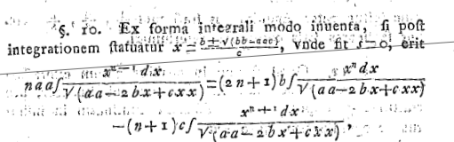
Figure 1.6: Euler and the Legendre Polynomials

Taken from [E606]. Euler solved the difference equation in terms of an integral. He was interested in the continued fraction of two consecutive Legendre polynomials. Thus, he did not find any of their more interesting properties, e.g., their orthogonality relation. This had to wait until Legendre’s paper [Le85].

Further, it seems that he did not notice the connection between the findings of [E551] published in 1783 and [E606] published in 1782. In other words, he was not aware that he already obtained an explicit formula for $P_{n}(x)$. This is even more interesting, because in [E551] he said that it is not possible for him to find such an explicit formula, although he provided all necessary tools in his earlier papers in 1750 in [E123] and in 1785 in [E594]. In summary, it seems that Euler was not aware that in those papers he basically discovered a general method to find a particular solution of the general homogeneous difference equation with linear coefficients.

1.5.3.3 2. Example: Hermite Polynomials

The Hermite polynomials satisfy the recurrence relation

$$H_{n+1}(x)=2xH_{n}(x)-2nH_{n-1}(x)$$

with the additional conditions $H_{0}(x)=1$, $H_{1}(x)=2x$. We then have the formula

Theorem 1.5.3 (Explicit Formula for the $n$-th Hermite Polynomial).

The following formula holds:

$$H_{n}(x)=\dfrac{i^{n}e^{x^{2}}}{2\sqrt{\pi}}\int\limits_{-\infty}^{\infty}t^{n}e^{\frac{1}{2}\left(-\frac{t^{2}}{2}-2xit\right)}dt$$

Proof.

We use the moment ansatz. We will not carry out the calculation since it is similar to the case of the Legendre polynomials. We will only state the intermediate results.
Of course, we start from the auxiliary equation:

$$\int\limits^{t}t^{n+1}P(t)dt=2x\int\limits^{t}t^{n}P(t)dt-2n\int\limits^{t}t^{n-1}P(t)dt+t^{n}Q(t).$$

From this we derive the following equations for $P(t)$ and $Q(t)$:

$$\begin{array}[]{llllllllll}1.&P(t)&\leavevmode\nobreak\ =\nobreak\leavevmode&\dfrac{Q^{\prime}(t)t}{t^{2}-2xt}\\ 2.&P(t)&\leavevmode\nobreak\ =\nobreak\leavevmode&\dfrac{Q(t)}{2},\end{array}$$

whence

$$Q(t)=C(x)e^{\frac{1}{2}\left(\frac{t^{2}}{2}-2xt\right)}\quad\text{and}\quad P(t)=\dfrac{1}{2}C(x)e^{\frac{1}{2}\left(\frac{t^{2}}{2}-2xt\right)}$$

In order to find the limits of integration, we need to solve $t^{n}e^{\frac{1}{2}\left(\frac{t^{2}}{2}-2xt\right)}=0$, which leads to $t=\pm i\infty$, if we want $n$ to be an arbitrary integer number. Therefore, up to this point we have:

$$H_{n}(x)=\dfrac{C(x)}{2}\int\limits_{-i\infty}^{i\infty}t^{n}e^{\frac{1}{2}\left(\frac{t^{2}}{2}-2xt\right)}dt.$$

It is convenient to get rid of the imaginary limits by the substitution $t=iy$. This gives

$$H_{n}(x)=\dfrac{C(x)}{2}i^{n+1}\int\limits_{-\infty}^{\infty}y^{n}e^{\frac{1}{2}\left(-\frac{y^{2}}{2}-2xiy\right)}dy.$$

From the initial condition $H_{0}(x)=1$ we find

$$\dfrac{C(x)}{2}=\dfrac{e^{x^{2}}}{2i\sqrt{\pi}}.$$

Therefore, we arrive at

$$H_{n}(x)=\dfrac{e^{x^{2}}i^{n}}{2\sqrt{\pi}}\int\limits_{-\infty}^{\infty}t^{n}e^{\frac{1}{2}\left(-\frac{t^{2}}{2}-2itx\right)}dt.$$

The condition $H_{1}(x)=2x$ is easily checked to be satisfied by the explicit formula. It is obvious that one can find similar explicit formulas for other orthogonal polynomials defined by second order homogeneous difference equations with linear coefficients, like, e.g., the Laguerre and Chebyshev polynomials. ∎

1.5.3.4 3. Example: Beta Function

Let us consider the $B$-function, which is defined as

Definition 1.5.1 ($B$-function).

The $B$-function, also referred to as Eulerian integral of the first kind, is defined as:

$$B(x,y):=\int\limits_{0}^{1}t^{x-1}(1-t)^{y-1}dt\quad\text{for}\quad\operatorname{Re}x,\operatorname{Re}y>0$$

From its definition it is immediate that $B$ satisfies the functional equation

$$B(x+1,y)=\dfrac{x}{x+y}B(x,y)\quad(*).$$

And one could start from this functional equation to obtain the integral representation via the moment ansatz. Euler did this in 1785 in $\S$ 17 of [E594]. Having already given several examples of this method, we do not want to do this here.
Here we want to use the results obtained up to this point to show:

Theorem 1.5.4.

We have

$$B(x,y)=\dfrac{\Gamma(x)\Gamma(y)}{\Gamma(x+y)}.$$

Proof.

We start from the functional equation $(*)$, of course. Further, we assume that $B$ can be written as product of two functions $B_{1}$, $B_{2}$. We demand those to satisfy the equations:

$$B_{1}(x+1,y)=xB_{1}(x,y)\quad\text{and}\quad(x+y)B_{2}(x+1,y)=B_{2}(x,y).$$

For the sake of brevity, we will drop the $y$ in the argument in the following; we consider the functional equation only in $x$, and $y$ can be seen as a parameter.
It is easily seen that $B_{1}(x)\cdot B_{2}(x)$ satisfies the functional equation for $B(x,y)$. Therefore, we need to solve the equations for $B_{1}$ and $B_{2}$ to find an expression for $B(x,y)$.
Let us consider $B_{1}$ first. It satisfies the functional equation of the $\Gamma$-function in $x$. Therefore, we immediately have

$$B_{1}(x)=C_{1}(y)\Gamma(x)\omega_{1}(x),$$

$C_{1}(y)$ being an arbitrary function of $y$, $\omega_{1}(x)$ being a periodic function with period $+1$.
To solve the functional equation for $B_{2}(x)$, let us introduce $D(x)=\frac{1}{B_{2}(x)}$. Then, $D(x)$ satisfies the functional equation:

$$D(x+1)=(x+y)D(x).$$

This equation is easily seen to be solved by

$$D(x)=C_{2}(y)\Gamma(x+y)\cdot\omega_{2}(x).$$

$C_{2}(y)$ is an arbitrary function of $y$, $\omega_{2}(x)$ being a periodic function of period $1$. And hence

$$B_{2}(x)=\dfrac{1}{C_{2}(y)\Gamma(x+y)}.$$

Combining the results, we have found

$$B(x,y)=\omega_{1}(x)\omega_{2}(x)C(y)\dfrac{\Gamma(x)}{\Gamma(x+y)},$$

where $C(y)=\frac{C_{1}(y)}{C_{2}(y)}$.
We can omit the periodic factor in this solution, since otherwise we would have:

$$B(x,y)=\int\limits_{0}^{1}dtt^{x-1}(1-t)^{y-1}=\Omega_{1}(x)\dfrac{\Gamma(x)\Gamma(y)}{\Gamma(x+y)},$$

where $\Omega_{1}(x)$ is a function with period $1$. But $\Omega_{1}(x)$ can be found from the special case $B(x,1)$. For, in this case we have on the one hand

$$B(x,1)=\int\limits_{0}^{1}dtt^{x-1}=\dfrac{1}{x}.$$

But on the other hand

$$B(x,1)=\dfrac{\Gamma(x)}{\Gamma(x+1)}\Omega_{1}(x)=\dfrac{\Omega_{1}(x)}{x}.$$

Here we used the functional equation of the $\Gamma$-function and $\Gamma(1)=1$. This already implies $\Omega_{1}(x)=1$ for all $x$. Hence the periodic function is simply $=1$.
It remains to determine the function $C(y)$. From the definition of $B(x,y)$ we find:

$$B(1,y)=\int\limits_{0}^{1}(1-t)^{y-1}dt=\dfrac{1}{y}.$$

First, from our solution we find

$$B(1,y)=C(y)\dfrac{\Gamma(1)}{\Gamma(y+1)}=C(y)\dfrac{1}{y\cdot\Gamma(y)},$$

where we used $\Gamma(1)=1$ and $\Gamma(y+1)=y\Gamma(y)$. Therefore, $C(y)$ must satisfy:

$$C(y)\dfrac{1}{y\Gamma(y)}=\dfrac{1}{y}\quad\text{or}\quad C(y)=\dfrac{1}{\Gamma(y)}.$$

Therefore, we finally arrived at the formula:

$$B(x,y)=\dfrac{\Gamma(x)\Gamma(y)}{\Gamma(x+y)}.$$

∎

1.5.3.5 Some Remarks on the Relation of $\Gamma$ and $B$.

The relation among the $B$- and $\Gamma$-function was already discovered by Euler essentially in 1738 in [E19]. He states it explicitly, e.g., in 1772 in [E421]. But the argument he gave there is not a rigorous proof, as we mentioned above in section 1.2.3, he only proved the formula for integers $x$ and $y$ and then, without any further explanation, replaced the factorials by the integral representation of $\Gamma(x)$.
Rigorous proofs were first given by Jacobi in 1834 in [Ja34] and Dirichlet in 1839 in [Di39], but they both use the theory of double integrals, which Euler did not know. We will discuss Euler’s argument, Dirichlet’s and Jacobi’s proof below in section LABEL:subsubsec:_Euler's_Proof, in section LABEL:subsubsec:_Dirichlet's_Proof and in section LABEL:subsubsec:_Jacobi's_Proof, respectively.
Our reasoning to obtain this fundamental relation does not require double integrals and our proof certainly was within Euler’s grasp. In [E594], he even considered similar questions, but never made the connection to the $B$- and $\Gamma$-functions.

1.5.3.6 4. Example: Hypergeometric Series

Finally, let us mention the hypergeometric series. It was first defined by Euler in [E710], a paper published only in 1801,

Definition 1.5.2 (Hypergeometric Series).

For $a,b,c\in\mathbb{C}\setminus\{{0,-1,-2,-3,\cdots\}}$ the hypergeometric series is defined by

$${}_{2}F_{1}(a,b,c;z)=1+\dfrac{ab}{c}\dfrac{z}{1!}+\dfrac{a(a+1)b(b+1)}{c(c+1)}\dfrac{z^{2}}{2!}+\cdots\quad\text{for}\quad|z|<1.$$

We will drop the subscripts $2$ and $1$, and write simply $F$, if there is no chance for confusion.
The first systematic study was done by Gauß in 1812 in [Ga28], whence the above series is often referred to as Gaussian hypergeometric series. Many people contributed to the nowadays highly developed theory of this function. We mention Kummer [Ku36] and Riemann [Ri57] as some of the contributors. The Gaußian hypergeometric series has been generalized in several ways. The number of parameters in the coefficients has been increased, leading to the Tomae functions ${}_{p}F_{q}$, see, e.g., [Sl09]. The number of variables has been increased, e.g., leading to Lauricella functions, which are also discussed in [Sl09]. Furthermore, we want to mention the GKZ systems and the modern text [Yo97]. Here we are mainly interested in hypergeometric integrals. A modern treatise on the subject is [Ao11]. What is of interest for us is that one can derive the integral representation of the hypergeometric series which is usually attributed to Euler from a certain difference equation which is satisfied by the the hypergeometric series. Gauß in his paper called them contiguity relations and gave a complete list of 15 of such equations. We will need one equation that follows from those he gave in the mentioned paper.

Theorem 1.5.5.

We have the following equation:

$$\begin{array}[]{lll}B(b+2,c-b){}F(a,b+2,c+2;x)&\leavevmode\nobreak\ =\nobreak\leavevmode&\left(\dfrac{b}{x(a-c-1)}\right)B(b,c-b)F(a,b,c;x)\\ &\leavevmode\nobreak\ +\nobreak\leavevmode&\left(\dfrac{(b-a+1)x+c}{x(c-a+1)}\right)B(b+1,c-b)F(a,b+1,c+1;x)\end{array}$$

The proof is simply done by expanding each hypergeometric function into a power series and comparing coefficients. We will not do this here. We will consider the above equation as an equation in $b$. Note that by dividing both sides by $B(b,c-b)$ and applying the relation to the $\Gamma$-function and its functional equation, the coefficients become linear functions in $b$. Then, it is a homogeneous difference equation with linear coefficients: $a,c,x$ are considered as parameters. Thus, we can solve this equation by the moment ansatz. Indeed, proceeding as in the previous cases (with the condition $F(a,0,c;x)=1$), after a long and tedious calculation we arrive at:

$$F(a,b,c;x)=\dfrac{\Gamma(c)}{\Gamma(a)\Gamma(c-b)}\int\limits_{0}^{1}t^{b-1}(1-t)^{c-b-1}(1-xt)^{-a}dt.$$

This is the Eulerian integral representation of the hypergeometric series.

Finally, let us mention one drawback of the moment ansatz. In Gauß’s paper one also finds contiguous relations, relating $F(a,b,c;x)$, $F(a+1,b,c;x)$ and $F(a-1,b,c;x)$ (see, e.g. equation [1] in $\S 7$ of [Ga28]). The coefficients are also linear in $a$. But in this case the moment ansatz does not produce a nice solution, if one just uses the ansatz

$$\int t^{a-1}P(t)dt,$$

since $P(t)$, as we have seen, also depends on $a$.

1.5.3.7 Historical Note on the Integral Representation

We wish to make some remarks on the origin of the the integral representation of the hypergeometric function. It is often ascribed to Euler that he found this representation, see, e.g., [An10], but it is actually not that simple. What can be said for certain is that we do not find the above equality explicitly in any of Euler’s publications. Therefore, let us briefly discuss, what Euler actually did.
First, as we already mentioned in the previous section, Euler studied the hypergeometric series in its most general form and defined it as the power series above in [E710], a paper written in 1778, but just published in 1801.
He proceeded to find the differential equation satisfied by it and found a transformation, now bearing his name, of the hypergeometric series in that paper. But he did NOT state the above integral representation anywhere. Nevertheless, on several instances, he did more general investigations, from which the formula would easily follow. Those investigations were mainly concerned with differential equations. We mention his 1763 paper [E274] and especially chapter 12 of his second book on integral calculus [E366] published in 1769. In both works, he derived differential equations for parameter integrals, depending on one ore more variables, by differentiating them under the integral sign.
His paper on the hypergeometric series, [E710], was written later, but nevertheless he did not make the connection to his earlier investigations. In conclusion, Euler could have written down the above equation, but he did not do so in any of his works.
Therefore, let us turn to the people, who actually stated the integral representation. The first to write down the integral representation appears to be Legendre in 1817 in [Le17], although Abel in 1827 in [Ab27] is often credited for it, confer, e.g., [Ni05]. Kummer also found it in 1837 in [Ku37a] and [Ku37b]. In those papers, he gave a general method to convert certain integrals into series and vice versa.
Having mentioned all this, it seems to be up to personal preference to call the integral formula the Eulerian integral representation or not.

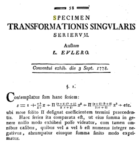
Figure 1.7: Euler and the hypergeometric Series

Definition of the hypergeometric series by Euler in [E710].

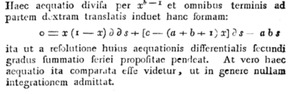
Figure 1.8: Euler and the hypergeometric Differential Equation

Euler finds the differential equation for the hypergeometric series in [E710].

Figure 1.9: Integral Representation of the hypergeometric Series

Euler got close to the integral representation of the hypergeometric series, taken from chapter 10 of [E366]. For a suitable choice of variables and after some simple substitutions, one arrives at the desired formula. Euler never related this result to the findings in [E710], the paper containing the first ever definition of the hypergeometric series as a power series.

1.5.4 Euler and the Mellin-Transform

1.5.4.1 Definition of the Mellin-Transform and inverse Mellin-Transform

Euler’s ansatz

$$F(x)=\int\limits_{a}^{b}t^{x-1}P(t)dt$$

for the solution of a homogeneous difference equation with linear coefficients bears quite a resemblance to the Mellin-Transform of a function $f(x)$. The Mellin-Transform $M(f)(s)$ is defined as

$$M(f)(s):=\int\limits_{0}^{\infty}t^{s-1}f(t)dt,$$

provided the integral exists. Although in Euler’s approach we had to calculate the limits of integration, we will argue that Euler’s method can be considered as a precursor of the Mellin-Transform, a concept introduced by Mellin in his 1895 paper [Me95]. To this end, let us introduce the Mellin-Transform properly.

Definition 1.5.3 (Mellin-Transform).

Let $t^{s-1}f(t)\in L^{1}(0,\infty)$, then the Mellin-Transform of the function $f$ is defined as:

$$F(s):=\int\limits_{0}^{\infty}t^{s-1}f(t)dt.$$

The inverse Mellin-Transform allows to recover the function $f$ from its Mellin-Transform. We have the

Theorem 1.5.6 (Inverse Mellin-Transform).

If $F(s)=\int\limits_{0}^{\infty}t^{s-1}f(t)dt$ exist, then we have

$$f(t)=\dfrac{1}{2\pi i}\int\limits_{c-i\infty}^{c+\infty}F(s)(t)^{-s}ds$$

with $c>0$, provided the integral exists.

We omit the proof here and refer the interested reader, e.g., to [Ti48]. We will not use this formula, but just stated it for the sake of completeness. Obviously, one can apply the inverse Mellin-Transform to find the function $P(t)$ in his ansatz. Thus, Euler’s method to find the function $P(t)$ is also a method to find the inverse Mellin-Transform.
In this section, we want to show that one can also start from the differential equation satisfied by $P(t)$ and using Euler’s ansatz one can recover the difference equation. We want to do this in Eulerian fashion and consider several examples of increasing complexity.
Before doing so, let us state the following theorem in advance:

Theorem 1.5.7.

Let $P(t)t^{s-1-n}\in L^{1}(0,\infty)$, $P\in\mathcal{C}^{n}(\mathbb{R})$ and $n\in\mathbb{N}$ a fixed natural number. If

$$F(s)=\int\limits_{0}^{\infty}t^{s-1}P(t)dt,$$

then

$$\int\limits_{0}^{\infty}t^{s-1}P^{(n)}(t)dt=(-1)(s-1)(s-2)\cdots(s-n)F(s-n).$$

The proof is by induction and integration by parts.

1.5.4.2 1. Example: $\Gamma$-function

Let us start with the most familiar example of a Mellin-Transfrom. We want to solve the equation

$$\Gamma(x+1)=x\Gamma(x)\quad\text{with}\quad\Gamma(1)=1\quad\text{for}\quad x>0$$

again. To this end, we start from the differential equation

$$P(t)=-P^{\prime}(t)$$

at which we arrived using Euler’s method in section 1.5.2.1. Thus, multiplying this equation by $t^{x}$ and integrating from $0$ to infinity, formally

$$\int\limits_{0}^{\infty}t^{x}P^{\prime}(t)dt=-\int\limits_{0}^{\infty}t^{x}P(t)dt,$$

whence by theorem 2.5.7

$$-x\int\limits_{0}^{\infty}t^{x-1}P(t)dt=-\int\limits_{0}^{\infty}t^{x}P(t)dt.$$

Therefore, calling $\Gamma(x)=\int\limits_{0}^{\infty}t^{x-1}P(t)dt$, we recover the equation

$$\Gamma(x+1)=x\Gamma(x).$$

Since the differential equation for $P$ is solved by $P(t)=Ce^{-t}$ with $C\neq 0$, as we also saw above, using the initial condition $\Gamma(1)=1$, we arrive at the integral representation of the $\Gamma$-function again.

1.5.4.3 Remark

Therefore, we used the differential equation, we found for $P(t)$ via the moment ansatz to reconstruct the difference equation we wanted to solve.
Generally speaking, we used that the Mellin-Transform converts a differential equation into a difference equation. Thus, vice versa the inverse Mellin-Transform converts a difference equation into a differential equation, which turned out to be the differential equation equation that we found using Euler’s method. The latter even works for general limits of integration as we will see in the following examples, whereas the Mellin-Transform is actually just defined for the limits $0$ and $\infty$.

1.5.4.4 2. Example: Generalized $\Gamma$-function

We now want to solve the difference equation

$$f(x+1)=(\alpha x+\beta)f(x)\quad\text{with},\quad f(1)=1,\alpha>0,\beta>0\quad\text{for}\quad x>0.$$

One can use Euler’s method again to solve this difference equation or simply guess the solution. Either way, the solution is given by

$$f(x)=C\int\limits_{0}^{\infty}t^{x-1+\frac{\beta}{\alpha}}e^{-\frac{t}{\alpha}}dt.$$

Thus, one finds that $P(t)=Ct^{\frac{\beta}{\alpha}}e^{-\frac{t}{\alpha}}$ in the moment ansatz. The constant $C$ is not important at the moment. We will determine it later in section 1.6.5. $P$ satisfies the following the differential equation:

$$P^{\prime}(t)\cdot t\alpha=\beta P(t)-tP(t).$$

Now assume that we did not know about the origin of that equation and we wanted to derive the corresponding difference equation. To this end, we multiply both sides by $t^{x-1}$ and integrate from $0$ to $\infty$:

$$\alpha\int\limits_{0}^{\infty}t^{x}P^{\prime}(t)dt=\beta\int\limits_{0}^{\infty}t^{x-1}P(t)dt-\int\limits_{0}^{\infty}t^{x}P(t)dt.$$

By theorem 2.5.7, this simplifies to

$$-x\alpha\int\limits_{0}^{\infty}t^{x-1}P(t)dt=\beta\int\limits_{0}^{\infty}t^{x-1}P(t)dt-\int\limits_{0}^{\infty}t^{x}P(t)dt.$$

Introducing $f(x)=\int\limits_{0}^{\infty}t^{x-1}P(t)dt$, the equation reads.

$$-x\alpha f(x)=\beta f(x)-\alpha f(x+1)$$

or, equivalently

$$f(x+1)=(\alpha x+\beta)f(x),$$

which is the initial difference equation again.
In the next example we want to see how one can derive the limits of integration, if they are not known in advance.

1.5.4.5 3. Example: Hermite Polynomials

We start from the differential equation

$$P(t)(t-2x)=2P^{\prime}(t),$$

multiply it by $t^{n}$, and integrate over $t$ from $a$ and $b$:

$$\int\limits_{a}^{b}P(t)t^{n+1}dt-2x\int\limits_{a}^{b}P(t)t^{n}dt=2\int\limits_{a}^{b}t^{n}P^{\prime}(t)dt.$$

Since theorem 2.5.7 only holds for $a=0$ and $b=\infty$, we have to keep the absolute part while integrating the right-hand side by parts:

$$\int\limits_{a}^{b}P(t)t^{n+1}dt-2x\int\limits_{a}^{b}P(t)t^{n}dt=\left.2t^{n}P(t)\right|_{a}^{b}-2n\int\limits_{a}^{b}t^{n-1}P(t)dt.$$

Introducing the notation $H_{n}(x)=\int\limits_{a}^{b}P(t)t^{n+1}dt$, we have:

$$H_{n+1}(x)-2xH_{n}(x)=\left.2t^{n}P(t)\right|_{a}^{b}-2nH_{n-1}(x).$$

Therefore, to recover the difference equation for the Hermite polynomials, see section 1.5.3.3, it has to be:

$$0=\left.2t^{n}P(t)\right|_{a}^{b}\quad\text{or}\quad 0=b^{n}P(b)-a^{n}P(a)\quad n\in\mathbb{N}.$$

Furthermore, we require $a\neq b$, since this solution is trivial. As we also saw in 1.5.3.3, $P(t)$ is given by

$$P(t)=C(x)e^{\frac{t^{2}}{4}-tx}.$$

$C(x)$ is just the integration constant. Therefore, a solution of the above equation is given by

$$(a,b)=(-i\infty,+i\infty),$$

whence, proceeding with this result, we recover the solution found in 1.5.3.3.
Therefore, we actually do not need Euler’s auxiliary function $Q(t)$ to find the limits of integration, but can also use the function $P(t)$ to do so.

1.5.4.6 4. Example: Legendre Polynomials

Finally, let us reconsider the Legendre polynomials already discussed in 1.5.3.1. We start from the differential equation

$$R^{\prime}(t)(t-2xt^{2}+t^{3})=(1-tx)R(t),$$

multiply it by $t^{n-2}$, and then integrate it from $a$ to $b$, whence:

$$\int\limits_{a}^{b}R^{\prime}(t)(t^{n-1}-2xt^{n}+t^{n+1})dt=\int(t^{n-2}-t^{n-1}x)R(t)dt.$$

Integration by parts on the left-hand side yields:

$$\left.R(t)t^{n-1}(t^{2}-2xt+1)\right|_{a}^{b}-\int\limits_{a}^{b}R(t)((n-1)t^{n-2}-2xnt^{n-1}+(n+1)t^{n})dt=\int\limits_{a}^{b}R(t)(t^{n-2}-t^{n-1}x)dt.$$

We want the absolute terms to vanish; using the explicit formula for $R(t)$ from 1.5.3.1, i.e. $\frac{t}{\sqrt{1-2xt+t^{2}}}$, this implies:

$$0=b^{n}\sqrt{1-2xb+b^{2}}-a^{n}\sqrt{1-2xa+a^{2}}\quad\forall n\in\mathbb{N}.$$

A solution, aside from $a=b$, is given by

$$(a,b)=\left(x-\sqrt{x^{2}-1},x+\sqrt{x^{2}+1}\right),$$

which is found, if each term in the above condition is set $=0$. Finally, let us introduce the notation $P_{n}(x)=\int\limits_{a}^{b}t^{n-1}P(t)dt$ with the solutions we just found for $a$ and $b$. Hence we arrive at

$$-(n-1)P_{n-1}(x)+2xnP_{n}(x)-(n+1)P_{(}n+1)(x)=P_{n-1}(x)-xP_{n}(x),$$

which, after some rearrangement, reads as:

$$(n+1)P_{n+1}(x)=(2n+1)xP_{n}(x)-nP_{n-1}(x)$$

which is the difference equation from which we started in 1.5.3.1.

1.5.4.7 Final Results

The examples we reconsidered illustrate lucidly that Euler, in some sense, anticipated the Mellin-Transform and found a way to calculate the inverse Mellin-Transform without using contour integration. As we already indicated, Euler’s approach is more general then Mellin’s, since Euler’s method works for general limits of integration.
Moreover, it is now evident that Euler’s results obtained via the moment ansatz can be justified rigorously using the theory of the Mellin-Transform and therefore, Euler’s results are indeed correct. And Euler’s momentum method is not just a precursor of the Mellin-Transform, but it is actually the same idea. Euler just discovered it in a completely different context, i.e. the solution of difference equations, see section 1.5.2, whereas Mellin introduced it in his studies of the hypergeometric differential equation. see, e.g., Mellin’s paper [Me95].

1.5.5 Modern Idea - Intersection Theory

Euler’s approach, referred to as moment method in section 1.5.2, started from the propounded difference equation and reduced it to a differential equation, whereas the Mellin-Transform approach outlined in section 1.5.4 started from a differential equation and derived the initially propounded difference equation. In this section, we want to introduce another method; it starts from a hypergeometric integral of the Eulerian type, i.e.

$$I=\int_{\mathcal{C}}t^{n-1}(1-t)^{\alpha}(1-xt)^{\beta}dt,\quad n,\alpha,\beta\in\mathbb{C}\setminus\mathbb{Z},$$

and derives a difference equation for it. We, following the treatise [Ao11], will briefly mention the fundamental theorems and ideas of the theory and give some examples, partially also found in [Fr19]. Before doing so, let us summarize the main ingredient of Euler’s approach.

1.5.5.1 Main Ingredient of Euler’s Approach

As mentioned in section 1.5.2, Euler explained his idea to solve homogeneous difference equations with linear coefficients in his 1750 paper [E123] $\S\S 49-53$, mainly focusing on continued fractions. But his main idea, aside from the ansatz

$$\int\limits_{a}^{b}t^{x-1}P(t)dt,$$

is the assumption of an auxiliary equation, i.e. adding the extra term $t^{x}Q(t)$. This was necessary to find the limits of integration. Then, we differentiated this auxiliary equation just to integrate it again later. Therefore, what we have essentially done, is to express the integral

$$\int\limits_{a}^{b}t^{x+1}P(t)dt$$

as a linear combination of one or two others of the same kind. More precisely, we found an equation

$$\int\limits_{a}^{b}t^{x+1}P(t)dt=C_{1}(x)\int\limits_{a}^{b}t^{x}P(t)dt+C_{2}(x)\int\limits_{a}^{b}t^{x-1}P(t)dt.$$

$C_{1}(x)$ and $C_{2}(x)$ are functions of $x$, linear in $x$ in our case. In physics, see, e.g., [Fr19], such equations are referred to as integration-by-parts-identities, or IBPs for short, and are frequently employed in the calculation of Feynman integrals of Feynman diagrams. The name IBP stems from the fact that the exponent of $t$ is lowered by $1$ by integrating by parts once.
Therefore, the extra term $t^{x}Q(t)$ can be understood as a term that has to be added to ensure that we arrive at the IBP given by the propounded difference equation. Intersection theory now turns this on its head and starts from an integral like the one above. It tells how many integrals of the same type one needs to express the given integral (e.g., it would immediately tell us that one requires two integrals to express $\int\limits_{a}^{b}t^{x+1}P(t)dt$) and furthermore it provides us with a tool to calculate the coefficients ($C_{1}(x)$ and $C_{2}(x)$ in our example).
But we will use it here to solve difference equations again, which will once more lead us to differential equations for the function $P(t)$. Thus, let us explain the origin of intersection theory first.

1.5.5.2 Overview

In the above integral, products of powers appear. Since we assume the powers to be non-integer numbers in general, we will modify de Rham’s theory presented in section 1.5.5.7, formalizing the ordinary theory of integrals of single-valued functions, to the multi-valued case. This modified de Rham theory, presented in section 1.5.5.8, is referred to as twisted de Rham theory. Since the key to ordinary de Rham theory is Stokes’ theorem, will we explain the analogue of this theorem for integrals of multi-valued functions first. We will do this in section 1.5.5.4.

1.5.5.3 Necessity for the Concept of a Twist

In this section, we want to motivate the concept of a twist. To this end, let $M$ be a $n$-dimensional affine variety obtained as the complement, in $\mathbb{C}^{n}$, of zeros $D_{j}:=\{P_{j}(u)=0\}$ of a finite number of polynomials $P_{j}(u)=P_{j}(u_{1},\cdots,u_{n})$, $1\leq j\leq m$; hence

$$M:=\mathbb{C}^{n}\setminus D,\quad D:=\bigcup\limits_{j=1}^{m}D_{j},$$

and consider the multi-valued function on $M$:

$$U(u)=\prod_{j=1}^{m}P_{j}(u)^{\alpha_{j}},\quad\alpha_{j}\in\mathbb{C}\setminus\mathbb{Z},\leavevmode\nobreak\ \leavevmode\nobreak\ 1\leq j\leq m.$$

Treating this $U(u)$, one way to get rid of its multi-valuedness such that the concepts of ordinary analysis can be applied to it, is to lift this $U$ to a covering manifold $\tilde{M}$ of $M$ and consider it on this $\tilde{M}$. But, in general the relation among $\tilde{M}$ and $M$ is so complicated that this approach is not preferable for practical calculations as we intend to perform them here.
Thus, instead of lifting $U$ to $\tilde{M}$, we introduce some quantities introducing a twist arising from the multi-valuedness, and then analyze $U$. In order to explain the key concepts as simply as possible, let us take a smooth triangulation $K$ on $M$. As mentioned earlier, we want to extend Stokes’ theorem to multi-valued differential forms $U\varphi$ with $\varphi\in\mathcal{A}^{\bullet}(M)$ and find the twisted version of de Rham’s theory afterwards.

1.5.5.4 Towards Stokes’ Theorem for Integrals of multi-valued Functions

We will argue rather intuitively, since the explanation of every mathematical detail is beyond the scope of this article. Let $\Delta$ be one of the $p$-simplexes of the smooth triangulation $K$ of $M$ and let $\varphi$ be a smooth $p$-form on $M$. To determine the integral of a multi-valued $p$-form we have to fix the branch of $U$ on $\Delta$. Then, we get to the following definition:

Definition 1.5.4.

Let the symbol $\Delta\otimes U_{\Delta}$ denote the pair of $\Delta$ and one of the branches $U_{\Delta}$ of $U$. Then, for $\varphi\in\mathcal{A}^{p}(M)$, the integral $\int\limits_{\Delta\otimes U_{\Delta}}U\cdot\varphi$ is defined as:

$$\int\limits_{\Delta\otimes U_{\Delta}}U\cdot\varphi:=\int\limits_{\Delta}\left[\text{the fixed branch }U_{\Delta}\text{ of }U\text{ on }\Delta\right]\cdot\varphi.$$

Since $U_{\Delta}$ can be continued analytically on a sufficiently small neighborhood of $\Delta$, on this neighborhood, for a single-valued $p$-form $U_{\Delta}\cdot\varphi$ and a $p$-simplex $\Delta$, the ordinary Stokes theorem holds and reads:

Theorem 1.5.8 (Stokes’s Theorem on $\Delta$).

For $\varphi\in\mathcal{A}^{p-1}(M)$ one has

$$\int\limits_{\Delta}d\left(U_{\Delta}\cdot\varphi\right)=\int\limits_{\partial\Delta}U_{\Delta}\cdot\varphi.$$

On the other hand, since

$$d\left(U_{\Delta}\cdot\varphi\right)=dU_{\Delta}\wedge\varphi+U_{\Delta}d\varphi=U_{\Delta}\left(d\varphi+\dfrac{dU_{\Delta}}{U_{\Delta}}\wedge\varphi\right)$$

on $\Delta$ and $\omega=\frac{dU}{U}$ is a single-value holomorphic $1$-form, setting

$$\nabla_{\omega}\varphi:=d\varphi+\omega\wedge\varphi,$$

we have:

$$d\left(U_{\Delta}\cdot\varphi\right)=U_{\Delta}\nabla_{\omega}\varphi.$$

$\nabla_{\omega}\varphi$ can be regarded as the defining equation of the covariant differential operator $\nabla_{\omega}$ associated to the connection form $\omega$. It satisfies $\nabla_{\omega}\cdot\nabla_{\omega}=0$ and in such a case $\nabla_{\omega}$ is said to be integrable or to define a Gauß-Manin connection of rank $1$ according to [De70]. Thus, we can rewrite Stokes’ theorem, using the symbol $\Delta\otimes U_{\Delta}$, as:

Theorem 1.5.9 (Stokes’ Theorem rewritten).

For $\varphi\in\mathcal{A}^{p-1}(M)$ we have:

$$\int\limits_{\Delta}d\left(U_{\Delta}\cdot\varphi\right)=\int\limits_{\Delta\otimes U_{\Delta}}U\cdot\nabla_{\omega}\varphi,$$

where

$$\nabla_{\omega}\varphi:=d\varphi+\omega\wedge\varphi\quad\text{and}\quad\omega=\dfrac{dU}{U}.$$

Next, we want to rewrite the right-hand side of the ordinary Stokes’ theorem (2.5.8). We will illustrate the idea by considering examples in low dimension.

1.5.5.5 Towards the twisted Homology Group

We start with the one-dimensional case. For an oriented $1$-simplex, with starting point $p$ and ending point $q$, and a smooth function (since $0$-forms are identified with functions) $\varphi$ on $M$, Stokes’ theorem (2.5.8.) becomes:

$$\int\limits_{\Delta}d\left(U_{\Delta}\cdot\varphi\right)=U_{\Delta}(q)\varphi(q)-U_{\Delta}(p)\varphi(p).$$

Here we have $\partial\Delta=\left\langle q\right\rangle-\left\langle p\right\rangle$ and $U_{\Delta}(q)$ is the value of the germ of the function $U_{q}$, determined by the branch $U_{\Delta}$ at the boundary $q$ of $\Delta$, at the point $q$.
Therefore, the symbol $\left\langle q\right\rangle\otimes U_{q}$ is determined and we have:

$$U_{\Delta}(q)\varphi(q)=\text{the integral of }U\cdot\varphi\text{ on }\left\langle q\right\rangle\otimes U_{q},$$

whence we conclude the formula:

$$\int\limits_{\Delta\otimes U_{\Delta}}U\cdot\nabla_{\omega}\varphi=\int\limits_{\left\langle q\right\rangle\otimes U_{q}-\left\langle p\right\rangle\otimes U_{p}}U\cdot\varphi.$$

Since, in the context of the rewritten Stokes theorem, the right-hand side is supposed to be the boundary of $\Delta\otimes U_{\Delta}$, we can define a boundary operator by:

Definition 1.5.5 (Boundary Operator for one dimensional $1$-simplex).

The boundary operator for this case can be defined as:

$$\partial_{\omega}(\Delta\otimes U_{\Delta}):=\left\langle q\right\rangle\otimes U_{q}-\left\langle p\right\rangle\otimes U_{p}.$$

Stokes’ theorem then reads:

$$\int\limits_{\Delta\otimes U_{\Delta}}U\cdot\nabla_{\omega}\varphi=\int\limits_{\partial_{\omega}(\Delta\otimes U_{\Delta})}U\cdot\varphi.$$

Let us also consider the two-dimensional case and let $\Delta$ be an oriented $2$-simplex with vertices $\left\langle 1\right\rangle$, $\left\langle 2\right\rangle$, $\left\langle 3\right\rangle$.

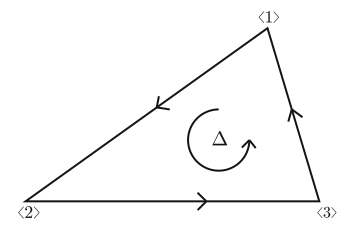
Figure 1.10: 2-simplex with Orientation in the two-dimensional Case

Auxiliary Figure for the determination of the boundary operator in the two-dimensional case. This is Figure 2.2 from [Ao11].

For a smooth $1$-form $\varphi$ on $M$, the right-hand side of the ordinary Stokes theorem reads:

$$\int\limits_{\partial\Delta}U_{\Delta}\cdot\varphi=\int\limits_{\left\langle 12\right\rangle}U_{\Delta}\cdot\varphi+\int\limits_{\left\langle 23\right\rangle}U_{\Delta}\cdot\varphi+\int\limits_{\left\langle 31\right\rangle}U_{\Delta}\cdot\varphi.$$

Let $U_{\left\langle 12\right\rangle}$ be the branch on the boundary $\left\langle 12\right\rangle$ of $\Delta$ determined by $U_{\Delta}$. Using the symbol $\left\langle 12\right\rangle\otimes U_{\left\langle 12\right\rangle}$, the above formula can be rewritten as follows:

$$\int_{\partial\Delta}U_{\Delta}\cdot\varphi=\int\limits_{\left\langle 12\right\rangle\otimes U_{\left\langle 12\right\rangle}}U\cdot\varphi+\int\limits_{\left\langle 23\right\rangle\otimes U_{\left\langle 23\right\rangle}}U\cdot\varphi+\int\limits_{\left\langle 31\right\rangle\otimes U_{\left\langle 31\right\rangle}}U\cdot\varphi.$$

This leads to the following definition of the boundary operator in this case:

Definition 1.5.6 (Boundary Operator for $2$-simplex in two-dimensional case).

The boundary operator in this case reads:

$$\partial_{\omega}(\Delta\otimes U_{\Delta}):=\left\langle 12\right\rangle\otimes U_{\left\langle 12\right\rangle}+\left\langle 23\right\rangle\otimes U_{\left\langle 23\right\rangle}+\left\langle 31\right\rangle\otimes U_{\left\langle 31\right\rangle}.$$

Hence Stokes’ theorem becomes:

$$\int\limits_{\Delta\otimes U_{\Delta}}U\cdot\nabla_{\omega}\varphi=\int\limits_{\partial(\Delta\otimes U_{\Delta})}U\varphi.$$

After these introductory examples, we can generalize them to the higher-dimensional case. Note that the boundary operators defined above are precisely those appearing in algebraic topology when one defines homology with coefficients in a local system. We will explain this below.
For now, consider the following differential equation on $M$

$$\nabla_{\omega}h=dh+\sum_{j=1}^{m}\alpha_{j}\dfrac{dP_{j}}{P_{j}}h=0$$

which has a general solution, formally expressible as:

$$h=c\prod_{j=1}^{m}P_{j}^{-\alpha_{j}},\quad c\in\mathbb{C}.$$

The space generated by the local solutions of the differential equation has dimension $1$. Cover the manifold $M$ by a sufficiently fine locally finite open cover $M=\cup U_{\nu}$ and fix a single-valued non-zero solution $h_{\nu}$ on each $U_{\nu}$. Since, provided $\mu\neq\nu$, $h_{\mu}$ and $h_{\nu}$ are solutions of the same differential function on the non-empty set $U_{\mu}\cap U_{\nu}$, setting

$$h_{\mu}(u)=g_{\mu\nu}(u)h_{\nu},\quad u\in U_{\mu}\cap U_{\nu}$$

the transition function $g_{\mu\nu}$ is a constant on $U_{\mu}\cap U_{\nu}$. Since a solution $h(u)$ on $U_{\mu}\cap U_{\nu}$ is expressed in two ways, i.e. as $h=\xi_{\mu}h_{\mu}=h=\xi_{\nu}h_{\nu}$ with $\xi_{\mu},\xi_{\nu}\in\mathbb{C}$, we find $\xi_{\mu}=g_{\mu\nu}^{-1}\xi_{\nu}$.
Therefore, the set of all local solutions of the given differential equation defines a flat line bundle $\mathcal{L}_{\omega}$ obtained by gluing the fibers $\mathbb{C}$ by the transition functions $\left\{g_{\mu\nu}^{-1}\right\}$. Let us denote the flat line bundle obtained from the transition functions $\left\{g_{\mu\nu}\right\}$ by $\mathcal{L}_{\omega}^{\vee}$ and call it the dual line bundle of the line bundle $\mathcal{L}_{\omega}$. By the above equation relating $h_{\nu}$ and $h_{\mu}$, $h_{\mu}^{-1}$ becomes a local section of $\mathcal{L}_{\omega}^{\vee}$. Moreover, from the initial differential equation, $\mathcal{L}_{\omega}^{\vee}$ can be considered as the flat line bundle generated by the set of all local solutions of

$$\nabla_{-\omega}h=dh-\sum_{j=1}^{m}\alpha_{j}\dfrac{dP_{j}}{P_{j}}h=0,$$

and $U(u)=\prod P_{j}^{\alpha_{j}}$ is its local section.
Often, e.g., in [Ao11], the term "flat line bundle" is used in the same sense as "system of rank $1$". Therefore, we call $\mathcal{L}_{\omega}^{\vee}$ the dual local system of $\mathcal{L}_{\omega}$. Hence we see that the boundary operators defined in the first two examples are those of the chain groups $C_{1}(K,\mathcal{L}_{\omega}^{\vee})$ and $C_{2}(K,\mathcal{L}_{\omega}^{\vee})$ with coefficients in $\mathcal{L}_{\omega}^{\vee}$. Naturally, if using $M$ instead of the simplicial complex $K$, we denote the chain group by $C_{q}(M,\mathcal{L}_{\omega}^{\vee})$ for the $q$-dimensional case. More precisely, we were lead to the definition:

Definition 1.5.7 ($p$-dimensional twisted Chain Group).

We call

$$C_{p}(M,\mathcal{L}_{\omega}^{\vee})=\left\{\begin{array}[]{l}\text{for a $p$-simplex $\Delta$ of $M$},\\ \text{the complex vector space}\\ \text{with basis $\Delta\otimes U_{\Delta}$}\end{array}\right\}$$

the $p$-dimensional twisted chain group.

Moreover, as a generalization of the above examples, we have:

Definition 1.5.8 (Boundary Operator of the $p$-simplex).

We define the boundary operator

$$\partial_{\omega}:C_{p}(M,\mathcal{L}_{\omega}^{\vee})\rightarrow C_{p-1}(M,\mathcal{L}_{\omega}^{\vee})$$

for the $p$-simplex $\Delta=\left\langle 012\cdots p\right\rangle$ as

$$\partial_{\omega}(\Delta\otimes U_{\Delta}):=\sum_{j=0}^{p}(-1)^{j}\left\langle 01\cdots\widehat{j}\cdots p\right\rangle\otimes U_{\left\langle 01\cdots\widehat{j}\cdots p\right\rangle}.$$

where $\widehat{j}$ indicates that this term is omitted.

Similarly to the ordinary homology theory, one has:

Theorem 1.5.10.

The boundary operator $\partial_{\omega}$ satisfies:

$$\partial_{\omega}\circ\partial_{\omega}=0.$$

Having given this theorem, we can define the twisted homology group:

Definition 1.5.9 (Twisted Homology Group).

The qoutient vector space

$$H_{p}(M,\mathcal{L}_{\omega}^{\vee}):=\left\{\text{Ker }\partial_{\omega}:C_{p}(M,\mathcal{L}_{\omega}^{\vee})\rightarrow C_{p-1}(M,\mathcal{L}_{\omega}^{\vee})\right\}/\partial_{\omega}C_{p+1}(M,\mathcal{L}_{\omega}^{\vee})$$

is called the $p$-dimensional twisted homology group, and an element of Ker $\partial_{\omega}$ is called a twisted cycle.

1.5.5.6 Locally finite Twisted Holonomy Group

Having arrived at the definition of the twisted homology group, we can now, in analogy to the ordinary homology group, introduce some related concepts. We start with the locally finite twisted homology group.
Since in general $M$ is not compact, it would require infinitely many simplices for its triangulation, hence it is natural to consider an infinite chain group which is locally finite. More precisely, we set:

Definition 1.5.10 (Locally finite $p$-dimensional twisted chain group).

The group

$$C_{p}^{lf}(M,\mathcal{L}_{\omega}^{\vee}):=\left\{\Sigma c_{\Delta}\Delta\otimes U_{\Delta}|\text{the $\Delta$'s are locally finite}\right\}$$

is called the locally finite Twisted chain Group.

Since $\partial_{\omega}\circ\partial_{\omega}=0$, $(C_{\bullet}^{lf}(M,\mathcal{L}_{\omega}^{\vee}))$ forms a complex, which in turn leads to the next

Definition 1.5.11 (Locally finite Twisted Holonomy Group).

The homology group obtained from the complex $(C_{\bullet}^{lf}(M,\mathcal{L}_{\omega}^{\vee}))$ is denoted by $(H_{\bullet}^{lf}(M,\mathcal{L}_{\omega}^{\vee}))$ and called the locally finite Twisted Holonomy Group.

Let us now consider Stokes’ theorem. Thus, let $\Delta$ be a $p$-simplex of $M$, $U_{\Delta}$ a branch of $U$ on $\Delta$, $\varphi\in\mathcal{A}^{p-1}(M)$, then the right-hand side of Stokes’ theorem becomes:

$$\begin{array}[]{lll}\int\limits_{\partial\Delta}U_{\Delta}\cdot\varphi&\leavevmode\nobreak\ =\nobreak\leavevmode&\sum_{i=0}^{p}(-1)^{i}\int\limits_{\left\langle 0\cdots\widehat{i}\cdots p\right\rangle}U_{\Delta}\cdot\varphi\\ &\leavevmode\nobreak\ =\nobreak\leavevmode&\sum_{i=0}^{p}(-1)^{i}\int\limits_{\left\langle 0\cdots\widehat{i}\cdots p\right\rangle\otimes U_{\left\langle 0\cdots\widehat{i}\cdots p\right\rangle}}U\cdot\varphi\\ &\leavevmode\nobreak\ =\nobreak\leavevmode&\int\limits_{\partial(\Delta\otimes U_{\Delta})}U\cdot\varphi.\end{array}$$

For a general twisted chain, one can just extend the definition $\mathbb{C}$-linearly and arrives at the following form of Stokes’ theorem:

Theorem 1.5.11 (Stokes’ Theorem for $C_{p}(M,\mathcal{L}_{\omega}^{\vee})$ and $C_{p}^{lf}(M,\mathcal{L}_{\omega}^{\vee})$).

• For $\sigma\in C_{p}(M,\mathcal{L}_{\omega}^{\vee})$ and $\varphi\in\mathcal{A}^{p-1}(M)$ we have:

  $$\int\limits_{\sigma}U\cdot\nabla_{\omega}\varphi=\int\limits_{\partial_{\omega}\sigma}U\cdot\varphi.$$

• For $\tau\in C_{p}^{lf}(M,\mathcal{L}_{\omega}^{\vee})$ and $\varphi\in\mathcal{A}_{c}^{p-1}(M)$ we have:

  $$\int\limits_{\tau}U\cdot\nabla_{\omega}\varphi=\int\limits_{\partial_{\omega}\tau}U\cdot\varphi.$$

Next, since we already see the similarity to the de Rham theory here, we want to construct the twisted version of the theory. To this end, using the last theorem, we have to establish relations among the cohomology of

$$\left(A^{\bullet}(M),\nabla_{\omega}\right),\quad\left(A_{p}^{\bullet}(M),\nabla_{\omega}\right)$$

and the twisted holonomy groups

$$H_{\bullet}\left(M,\mathcal{L}_{\omega}^{\vee}\right),\quad H_{\bullet}^{lf}\left(M,\mathcal{L}_{\omega}^{\vee}\right).$$

1.5.5.7 de Rham Theory

As mentioned in the preceding section, we want to establish that the cohomology of the complex $\left(A^{\bullet}(M),\nabla_{\omega}\right)$ is dual to the twisted homology $H_{\bullet}\left(M,\mathcal{L}_{\omega}^{\vee}\right)$. Since the proof of this fact is too long to present it here, we will simply state the theorem. The reader interested in the proof is, e.g., referred to [Ao11].
Furthermore, let us point out that ordinary de Rham theory corresponds to the case $\omega=0$ and thus twisted de Rham theory will be its natural generalization.
De Rham theory is summarized by de Rham’s theorem and duality theorems.

Theorem 1.5.12 (de Rham’s Theorem).

The following isomorphisms exist:

$$\begin{array}[]{ll}(1)&H^{p}(M,\mathbb{C})\simeq\left\{\begin{array}[]{c}H^{p}(\mathcal{A}^{\bullet}(M),d)\\ \uparrow\wr\\ H^{p}(\Omega^{\bullet}(M),d)\end{array}\right\}\xrightarrow{\sim}H^{p}(\mathcal{K}^{\bullet}(M),d)\xleftarrow{\sim}H_{2n-p}^{lf}(M,\mathbb{C})\\ (2)&H_{c}^{p}(M,\mathbb{C})\simeq H^{p}(\mathcal{A}_{c}^{\bullet}(M),d)\xrightarrow{\sim}H^{p}(\mathcal{K}_{c}^{\bullet}(M),d)\xleftarrow{\sim}H_{2n-p}(M,\mathbb{C}).\end{array}$$

Here, $\mathcal{K}_{c}^{p}$ is the sheaf of germs of currents of degree $p$ with compact support on $M$. A current is an element of the space containing both $\mathcal{C}^{\infty}$ differential forms and smooth singular chains.
Furthermore, we have the following

Theorem 1.5.13 (Duality Theorems).

The following bilinear forms are non-degenerate

$$\begin{array}[]{cccccccccccccc}(1)&H_{p}(M,\mathbb{C})&\leavevmode\nobreak\ \times\nobreak\leavevmode&H^{p}(\mathcal{A}^{\bullet}(M),d)&\leavevmode\nobreak\ \rightarrow\nobreak\leavevmode&\mathbb{C}\\ &&&(\left[\sigma\right],\left[\varphi\right])&\leavevmode\nobreak\ \longmapsto\nobreak\leavevmode&\int\limits_{\sigma}\varphi,\\ (2)&H^{2n-p}(\mathcal{A}_{c}^{\bullet}M,\mathbb{C})&\leavevmode\nobreak\ \times\nobreak\leavevmode&H^{p}(\mathcal{A}^{\bullet}(M),d)&\leavevmode\nobreak\ \rightarrow\nobreak\leavevmode&\mathbb{C}\\ &&&(\left[\alpha\right],\left[\beta\right])&\leavevmode\nobreak\ \longmapsto\nobreak\leavevmode&\int\limits_{M}\alpha\wedge\beta.\\ \end{array}$$

These are the fundamental theorems in de Rham theory. These results can be extended to twisted de Rham theory.

1.5.5.8 Twisted de Rham Theory

We state the most important theorems necessary to develop twisted de Rham theory

Theorem 1.5.14.

There is an natural isomorphism

$$H^{p}(M,\mathcal{L}_{\omega})\simeq\operatorname{Hom}_{\mathbb{C}}(H_{p}(M,\mathcal{L}_{\omega}^{\vee}),\mathbb{C})$$

Via this isomorphism, the cohomology group $H^{p}(M,\mathcal{L}_{\omega})$ can be considered as the dual space of the homology group $H_{p}(M,\mathcal{L}_{\omega}^{\vee})$. Therefore, the value $\left\langle\left[\sigma\right],\left[\varphi\right]\right\rangle$ of a cohomology class $\left[\varphi\right]\in H^{p}(M,\mathcal{L}_{\omega})$ at a homology class $\left[\sigma\right]\in H_{p}(M,\mathcal{L}_{\omega})$ is well-defined and we have the following

Theorem 1.5.15.

The following bilinear form is non-degenerate

$$\begin{array}[]{ccccccccc}H_{p}(M,\mathcal{L}_{\omega}^{\vee})&\leavevmode\nobreak\ \times\nobreak\leavevmode&H^{p}(M,\mathcal{L}_{\omega})&\leavevmode\nobreak\ \rightarrow&\mathbb{C}\\ &&\left(\left[\sigma\right],\left[\varphi\right]\right)&\leavevmode\nobreak\ \rightarrow\nobreak\leavevmode&\left\langle\left[\sigma\right],\left[\varphi\right]\right\rangle.\end{array}$$

In analogy to de Rham’s Theorem, we have the

Theorem 1.5.16.

The following isomorphisms exist

$$\begin{array}[]{ll}(1)&H^{p}(M,\mathcal{L}_{\omega})\simeq\left\{\begin{array}[]{c}H^{p}(\mathcal{A}^{\bullet}(M),\nabla_{\omega})\\ \uparrow\wr\\ H^{p}(\Omega^{\bullet}(M),\nabla_{\omega})\end{array}\right\}\xrightarrow{\sim}H^{p}(\mathcal{K}^{\bullet}(M),\nabla_{\omega})\xleftarrow{\sim}H_{2n-p}^{lf}(M,\mathcal{L}_{\omega})\\ (2)&H_{c}^{p}(M,\mathcal{L}_{\omega})\simeq H^{p}(\mathcal{A}_{c}^{\bullet}(M),\nabla_{\omega})\xrightarrow{\sim}H^{p}(\mathcal{K}_{c}^{\bullet}(M),\nabla_{\omega})\xleftarrow{\sim}H_{2n-p}(M,\mathcal{L}_{\omega}).\end{array}$$

Finally, we can give the most important theorem for our investigations.

Theorem 1.5.17.

The following bilinear forms are non-degenerate

$$\begin{array}[]{crccclcc}(1)&H_{p}(M,\mathcal{L}_{\omega}^{\vee})&\leavevmode\nobreak\ \times\nobreak\leavevmode&H^{p}(\mathcal{A}^{\bullet}(M),\nabla_{\omega})&\leavevmode\nobreak\ \rightarrow\nobreak\leavevmode&\mathbb{C}\\ &&&(\left[\sigma\right],\left[\varphi\right])&\leavevmode\nobreak\ \mapsto\nobreak\leavevmode&\int\limits_{\sigma}U\cdot\varphi.\\ (2)&H^{p}(\mathcal{A}_{c}^{\bullet}(M),\nabla_{\omega})&\leavevmode\nobreak\ \times\nobreak\leavevmode&H_{p}^{lf}(M),\mathcal{L}_{\omega}^{\vee})&\leavevmode\nobreak\ \rightarrow\nobreak\leavevmode&\mathbb{C}\\ &&&(\left[\psi\right],\left[\tau\right])&\leavevmode\nobreak\ \mapsto\nobreak\leavevmode&\int\limits_{\tau}U\cdot\psi.\\ (3)&H^{2n-p}(\mathcal{A}_{c}^{\bullet}(M),\nabla_{-\omega})&\leavevmode\nobreak\ \times\nobreak\leavevmode&H^{p}(\mathcal{A}^{\bullet}(M),\nabla_{\omega})&\leavevmode\nobreak\ \rightarrow\nobreak\leavevmode&\mathbb{C}\\ &&&(\left[\alpha\right],\left[\beta\right])&\leavevmode\nobreak\ \mapsto\nobreak\leavevmode&\int\limits_{M}\alpha\wedge\beta.\\ (4)&H_{p}(M,\mathcal{L}_{\omega}^{\vee})&\leavevmode\nobreak\ \times\nobreak\leavevmode&H_{2n-p}^{lf}(M,\mathcal{L}_{\omega})&\leavevmode\nobreak\ \rightarrow\nobreak\leavevmode&\mathbb{C}\\ &&&(\left[\sigma\right],\left[\tau\right])&\leavevmode\nobreak\ \mapsto\nobreak\leavevmode&\text{intersection number }\left[\sigma\right]\cdot[\tau].\end{array}$$

In the next sections we will explain the meaning of equation (4), i.e. the intersection number which is crucial for investigations of hypergeometric integrals.

1.5.5.9 Construction of twisted Cycles

In this section, we want to construct some twisted cycles explicitly. Starting from the one-dimensional case and the twisted cycle around one point, we will generalize this and will arrive at an explicit formula for $H_{1}(M,\mathcal{L}_{\omega}^{\vee})$.
We will explicitly construct $m-1$ independent twisted cycles associated to the multi-valued function

$$U(u)=\prod_{j=1}^{m}(u-x_{j})^{\alpha_{j}},\quad\alpha_{j}\notin\mathbb{Z}$$

which is defined $M=\mathbb{C}\setminus\{x_{1},\cdots,x_{m}\}$. Since later we will also be mainly interested in this case, we assume all the points $x_{j},\leavevmode\nobreak\ 1\leq j\leq m$ to lie on the real axis such that $x_{1}<\cdots<x_{m}$. We set $\omega=\frac{dU}{U}$ such that this $U$, as we explained in section 1.5.5.5, defines the rank $1$ local system $\mathcal{L}_{\omega}^{\vee}$. We choose the following branch of $U(u)$: we take the one that is single-valued on the lower half plane and that satisfies

$$\operatorname{arg}(u-x_{j})=\left\{\begin{array}[]{rl}0&(1\leq j\leq p)\\ -\pi&(p+1\leq j\leq m)\end{array}\right\}$$

on each interval $\Delta_{p}:=(x_{p},x_{p+1})$, $1\leq p\leq m-1$. From basic algebraic topology we know that
(1) $H_{\bullet}(M,\mathcal{L}_{\omega}^{\vee})$ is homotopy invariant
(2) The Mayer-Vietoris sequence holds
Thus, using (1) it suffices to calculate $H_{\bullet}(K,\mathcal{L}_{\omega}^{\vee})$ for the one-dimensional simplicial complex $K$ seen in the figure above. Note that, for the sake of simplicity, we also write $\mathcal{L}_{\omega}^{\vee}$ for the restriction of $\mathcal{L}_{\omega}^{\vee}$ on $M$ to $K$. To apply the Mayer-Vietoris sequence (2), let us write $K=K_{1}\cup K_{2}$, i.e. as the union of two subcomplexes

$$K_{1}=\bigcup_{j=1}^{m}S_{\varepsilon}^{1}(x_{j}),\quad K_{2}=\bigcup_{j=1}^{m-1}[x_{j}+\varepsilon,x_{j+1}-\varepsilon].$$

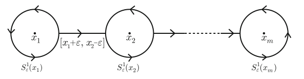
Figure 1.11: Construction of twisted Cycles in the one-dimensional Case

Auxiliary figure for the construction of a twisted cycles for the function $U(u)=\prod_{j=1}^{m}(u-x_{j})^{\alpha_{j}},\leavevmode\nobreak\ \alpha_{j}\notin\mathbb{Z}$. This is figure 2.5 from [Ao11].

In the first step, we calculate the twisted homology for each circle $S_{\varepsilon}^{1}(x_{j})$, i.e. we prove:

Theorem 1.5.18 (Twisted homology for a circle).

For $\alpha_{j}\notin\mathbb{Z}$, $1\leq j\leq m$, we have

$$H_{q}(S_{\varepsilon}^{1}(x_{j}),\mathcal{L}_{\omega}^{\vee})=0,\quad q=0,1,\cdots$$

Proof.

We triangulate the circle as seen in the figure above

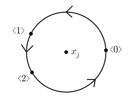
Figure 1.12: Triangulation of the Circle

Auxiliary figure for the calculation of $H_{q}(S_{\varepsilon}^{1}(x_{j}),\mathcal{L}_{\omega}^{\vee})$. This is figure 2.6 from [Ao11].

Thus, the chain group $C_{q}(S_{\varepsilon}^{1}(x_{j}),\mathcal{L}_{\omega}^{\vee})$ and the boundary operator $\partial_{\omega}$ are:

$$\begin{array}[]{l}C_{0}(S_{\varepsilon}^{1}(x_{j}),\mathcal{L}_{\omega}^{\vee})=\mathbb{C}\langle 0\rangle+\mathbb{C}\langle 1\rangle+\mathbb{C}\langle 2\rangle,\\ C_{1}(S_{\varepsilon}^{1}(x_{j}),\mathcal{L}_{\omega}^{\vee})=\mathbb{C}\langle 01\rangle+\mathbb{C}\langle 12\rangle+\mathbb{C}\langle 20\rangle,\\ \partial_{\omega}\langle 01\rangle=\langle 1\rangle-\langle 0\rangle,\quad\partial_{\omega}\langle 12\rangle=\langle 2\rangle-\langle 0\rangle,\quad\partial_{\omega}\langle 20\rangle=c_{j}\langle 0\rangle-\langle 2\rangle,\end{array}$$

with $c_{j}=\exp(2\pi i\alpha_{j})$. Writing these relations as a vectorial equation, we have

$$\partial_{\omega}\begin{pmatrix}\langle 01\rangle\\ \langle 12\rangle\\ \langle 20\rangle\end{pmatrix}=\begin{pmatrix}-1&1&0\\ 0&-1&1\\ c_{j}&0&-1\end{pmatrix}\begin{pmatrix}\langle 0\rangle\\ \langle 1\rangle\\ \langle 2\rangle\end{pmatrix}$$

and $\operatorname{det}(\partial_{\omega})=c_{j}-1$. This is not zero, since $\alpha_{j}\notin\mathbb{Z}$. Therefore, the map

$$\partial_{\omega}C_{1}(S_{\varepsilon}^{1}(x_{j}),\mathcal{L}_{\omega}^{\vee})\rightarrow C_{0}(S_{\varepsilon}^{1}(x_{j}),\mathcal{L}_{\omega}^{\vee})$$

is an isomorphism and hence the theorem is proven. ∎

Next, we have the

Theorem 1.5.19.

Provided $\alpha_{j}\notin\mathbb{Z}$, $1\leq j\leq m$, we have

$$\begin{array}[]{lcl}H_{0}(M,\mathcal{L}_{\omega}^{\vee})&\leavevmode\nobreak\ =\nobreak\leavevmode&0,\\ H_{1}(M,\mathcal{L}_{\omega}^{\vee})&\simeq\nobreak\leavevmode&\mathbb{C}\cdot\Delta_{j}(\omega)\end{array}$$

with the twisted cycle $\Delta_{j}(\omega)$

$$\Delta_{j}(\omega):=\dfrac{1}{c_{j}-1}S_{\varepsilon}^{1}(x_{j})+[x_{j}+\varepsilon,x_{j+1}-\varepsilon]-\dfrac{1}{c_{j+1}-1}S_{\varepsilon}^{1}(x_{j+1}).$$

We sketch the idea of the proof. One applies the Mayer-Vietoris sequence to the union $K=K_{1}\cup K_{2}$ to find the exact sequence

$$0\rightarrow H_{1}(K_{1},\mathcal{L}_{\omega}^{\vee})\oplus H_{1}(K_{2},\mathcal{L}_{\omega}^{\vee})\rightarrow H_{1}(K,\mathcal{L}_{\omega}^{\vee})\xrightarrow{\delta}$$

$$\rightarrow H_{0}(K_{1}\cap K_{2},\mathcal{L}_{\omega}^{\vee})\rightarrow H_{0}(K_{1},\mathcal{L}_{\omega}^{\vee})\oplus H_{0}(K_{2},\mathcal{L}_{\omega}^{\vee})\rightarrow H_{0}(K,\mathcal{L}_{\omega}^{\vee})\rightarrow 0.$$

Therefore, the task is to find $\delta$ such that one can determine $H_{1}(K,\mathcal{L}_{\omega}^{\vee})$. To this end, note that $K_{2}$ is homotopically equivalent to $m-1$ points and $K_{1}\cap K_{2}$ is homotopically equivalent to $2m-2$ points. Furthermore, using the last theorem, many terms in the sequence are seen to vanish, and we are left with the exact sequence:

$$\begin{array}[]{cccccccccccc}&0&\leavevmode\nobreak\ \rightarrow\nobreak\leavevmode&H_{1}(K,\mathcal{L}_{\omega}^{\vee})&\leavevmode\nobreak\ \xrightarrow{\delta}\nobreak\leavevmode&H_{0}(K_{1}\cap K_{2},\mathcal{L}_{\omega}^{\vee})&\leavevmode\nobreak\ \xrightarrow{i_{*}}\nobreak\leavevmode&H_{0}(K_{2},\mathcal{L}_{\omega}^{\vee})&\leavevmode\nobreak\ \rightarrow\\ &&&&&||\wr&&||\wr\\ &&&&&\mathbb{C}^{2m-2}&&\mathbb{C}^{m-1}\\ &&\leavevmode\nobreak\ \rightarrow\nobreak\leavevmode&H_{0}(K_{,}\mathcal{L}_{\omega}^{\vee})&\leavevmode\nobreak\ \rightarrow\nobreak\leavevmode&0\end{array}$$

The map $i_{*}$ is induced from he inclusion $i:K_{1}\cap K_{2}\rightarrow K_{2}$ and we find

$$i_{*}\left(\sum_{j=1}^{m-1}a_{j}\langle x_{j}+\varepsilon\rangle+b_{j}\langle x_{j+1}-\varepsilon\rangle\right)=\sum_{j=1}^{m-1}(a_{j}+b_{j})\langle x_{j}+\varepsilon\rangle,\quad a_{j},b_{j}\in\mathbb{C}.$$

Thus, $i_{*}$ is surjective and we find:

$$\begin{array}[]{llll}H_{0}(K,\mathcal{L}_{\omega}^{\vee})=0\\ \operatorname{Im}\delta=\operatorname{Ker}i_{*}=\bigoplus_{j=1}^{m-1}\mathbb{C}(\langle x_{j}-\varepsilon\rangle-\langle x_{j+1}-\varepsilon\rangle).\end{array}$$

One finds $\delta$, which is necessary to find $H_{1}(K,\mathcal{L}_{\omega}^{\vee})$, in the same way; we state the result. Defining

$$\Delta_{j}(\omega):=\dfrac{1}{c_{j}-1}S_{\varepsilon}^{1}(x_{j})+[x_{j}+\varepsilon,x_{j+1}-\varepsilon]-\dfrac{1}{c_{j+1}-1}S_{\varepsilon}^{1}(x_{j+1}),$$

one has

$$\delta(\Delta_{j}(\omega))=\langle x_{j}+\varepsilon\rangle-\langle x_{j+1}-\varepsilon\rangle$$

Therefore,

$$H_{1}(K,\mathcal{K}_{\omega}^{\vee})=\bigoplus_{j=1}^{m-1}\mathbb{C}\cdot\Delta_{j}(\omega).$$

1.5.5.10 Intersection Number for Twisted Cycles

We will explain the intersection number by means of a simple example which can then be generalized to the general case. First, we mention the

Theorem 1.5.20.

Under the assumption $\sum_{j=1}^{m}\alpha_{j}\notin\mathbb{Z}$, twisted cycles $\Delta_{\nu}\otimes U_{\Delta_{\nu}}$ defined by bounded chambers $\Delta_{\nu}$, $1\leq\nu\leq\binom{m-1}{n}$, form a basis of $H_{n}^{lf}(M,\mathcal{L}_{\omega}^{\vee})$:

$$H_{n}^{lf}(M,\mathcal{L}_{\omega}^{\vee})\simeq\bigoplus\limits_{\nu=1}^{\binom{m-1}{n}}\mathbb{C}\left[\Delta_{\nu}\otimes U_{\Delta_{\nu}}\right].$$

Concerning bounded champers: The arrangement of $m$ real hyperplanes in $\mathbb{R}^{n}$ decomposes that space into several chambers, which are referred to as bounded chambers.
Having stated this theorem in advance, let us explain what the intersection number between $H_{1}(M,\mathcal{L}_{\omega}^{\vee})$ and $H_{1}^{lf}(M,\mathcal{L}_{\omega}^{\vee})$ means. We will consider the case $m=2$, the general case can then be understood similarly.
Let $M=\mathbb{C}\setminus\{0,1\}$ and choose a branch of the multi-valued function $U(u)=u^{\alpha}(u-1)^{\beta}$, $\alpha,\beta,\alpha+\beta\notin\mathbb{Z}$. $H_{1}(M,\mathcal{L}_{\omega}^{\vee})$ is one dimensional and is basis is given by

$$\begin{array}[]{l}\Delta(\omega)=\dfrac{1}{c_{1}-1}S_{\varepsilon}^{1}(0)\otimes U_{S_{\varepsilon}^{1}(0)}+[\varepsilon,1-\varepsilon]\otimes U_{[\varepsilon,1-\varepsilon]}-\dfrac{1}{c_{2}-1}S_{\varepsilon}^{1}(1)\otimes U_{S_{\varepsilon}^{1}(1)},\\ c_{1}=\exp(2\pi i\sqrt{\alpha}),\quad c_{2}=\exp(2\pi i\beta)\end{array}$$

$S_{\varepsilon}^{1}(0)$ is a circle around $0$ with radius $p$ with starting point $\varepsilon$, which turns in anticlockwise direction, stopping at an infinitely near point before $\varepsilon$, and $U_{S_{\varepsilon}^{1}(0)}$ is the branch obtained by analytic continuation along $S_{\varepsilon}^{1}(0)$, and similarly for the rest.
Now, using the above theorem, $H_{1}^{lf}(M,\mathcal{L}_{\omega})$ is the one dimensional vector space with basis $(0,1)\otimes U_{(0,1)}^{-1}$, where $U_{(0,1)}$ is the restriction of the branch determined above to $(0,1)$. Define $\Delta:=\gamma\otimes U_{\gamma}^{-1}$, obtained by deforming the interval $(0,1)$ as in the figure above, this is homologous to $(0,1)\otimes U_{(0,1)}^{-1}$ in $H_{1}^{lf}(M,\mathcal{L}_{\omega})$.

The geometric intersections of $\Delta(\omega)$ and $\Delta$ are the three points $p$, $\frac{1}{2}$, $q$ and the signatures are $-$, $-$, $+$. Since the difference of the branches is cancelled by $U$ and $U^{-1}$, we finally arrive at:

$$\begin{array}[]{lll}\Delta(\omega)\cdot\Delta&\leavevmode\nobreak\ =\nobreak\leavevmode&\dfrac{1}{c_{1}-1}\times(-1)+(-1)+\left(-\dfrac{1}{c_{2}-1}\right)\times(+1)\\ &\leavevmode\nobreak\ =\nobreak\leavevmode&-\dfrac{c_{1}c_{2}-1}{(c_{1}-1)(c_{2}-1)}\end{array}$$

for the intersection number.

As already indicated, one can compute the intersection matrix for a general $m$ in a similar way. The result will look as follows: We set $\Delta_{j}:=(x_{j},x_{j+1})\otimes U_{(x_{j},x_{j+1})}^{-1}\in H_{1}^{lf}(M,\mathcal{L}_{\omega})$, $1\leq j\leq m-1$, $c_{j}=\exp(2\pi i\alpha_{j})$, $d_{j}:=c_{j}-1$, $d_{jk}=c_{j}c_{k}-1$, then we have:

$$\Delta_{j}(\omega)\cdot\Delta_{k}=\left\{\begin{array}[]{lll}\dfrac{c_{j}}{d_{j}},&j=k+1,\\ -\dfrac{d_{j,j+1}}{d_{j}d_{j+1}},&j=k,\\ -\dfrac{1}{d_{k}},&j+1=k\\ 0,&\text{otherwise}\end{array}\right.$$

Figure 1.13: Intersections of $\Delta(\omega)$ and $\Delta$

Figure showing the three intersection of $\Delta(\omega)$ and $\Delta$ at the three points $p$, $\frac{1}{2}$, $q$. This is Figure 2.7 from [Ao11].

Therefore, the intersection matrix, consisting of each intersection number, reads:

$$\begin{pmatrix}\Delta_{1}(\omega)\cdot\Delta_{1}&\cdots&\Delta_{1}(\omega)\cdot\Delta_{m-1}\\ \vdots&&\vdots\\ \Delta_{m-1}(\omega)\cdot\Delta_{1}&\cdots&\Delta_{m-1}(\omega)\cdot\Delta_{m-1}\end{pmatrix}$$

$$=-\begin{pmatrix}\dfrac{d_{12}}{d_{1}d_{2}}&\dfrac{-1}{d_{2}}&&0&\cdots&0&0\\ \dfrac{-c_{2}}{d_{2}}&\dfrac{d_{23}}{d_{2}d_{3}}&&&&0&0\\ &&&&&\vdots\\ 0&0&&&&\dfrac{d_{m-2,m-1}}{d_{m-2}d_{m-1}}&\dfrac{-1}{d_{m-1}}\\ 0&0&\cdots&&0&\dfrac{-c_{m-1}}{d_{m-1}}&\dfrac{d_{m-1,m}}{d_{m-1}d_{m}}\end{pmatrix}$$

1.5.5.11 Intersection Numbers for Twisted Cocycles

Although the intersection number of twisted cycles is of great importance in the general theory of hypergeometric functions, for us, more interested in difference equations, we need the intersection number of twisted cocycles. Above, in the main theorem of section 1.5.5.8, equation (3),

$$H^{n}(M,\mathcal{L}_{\omega})\times H_{c}^{n}(M,\mathcal{L}_{\omega}^{\vee})\rightarrow\mathbb{C}$$

can be considered to define an intersection number of twisted cocycles. Indeed, the calculation works similarly to the case of twisted cycles and was carried out explicitly in [Ch95] such that it will enough to mention the necessary definitions briefly and consider examples after this.
Here, we set $M=\mathbb{P}^{1}\setminus\{x_{0},\cdots,x_{m}\}$, where the case $x_{i}=\infty$ is not excluded. We define

$$\omega:=\sum_{j=0}^{m}\alpha_{j}\dfrac{du}{u-x_{j}},\leavevmode\nobreak\ \leavevmode\nobreak\ \nabla_{\omega}:=d+\omega\wedge,\leavevmode\nobreak\ \leavevmode\nobreak\ \nabla_{\omega}^{\vee}:=d-\omega\wedge$$

and let $D$ be the divisor of $\mathbb{P}^{1}$ determined by the $m+1$ points $x_{0},\cdots,x_{m}$, and denote the sheaf of logarithmic $p$-forms that may have logarithmic poles only along $D$ by $\Omega_{\mathbb{P}^{1}}^{p}(\log D)$ and the sub-sheaf of $\Omega_{\mathbb{P}^{1}}^{p}(\log D)$ of $p$-forms which have poles along $D$ of at least order $1$ by $\Omega_{\mathbb{P}^{1}}^{p}(\log D)(-D)$, then we have the

Theorem 1.5.21.

The following bilinear form is non-degenerate

$$I:\Gamma\left(\mathbb{P}^{1},\Omega_{\mathbb{P}^{1}}^{1}(\log D)\right)\times H^{1}(\mathbb{P}^{1},\mathcal{O}_{\mathbb{P}^{1}}(-D))\rightarrow\mathbb{C}.$$

This defines the intersection number

Definition 1.5.12 (Intersection Number for twisted Cocycles).

We define the intersection number of $\varphi^{+}$, $\psi^{-}$ by

$$I_{c}(\varphi^{+},\psi^{-}):=I(\varphi,i^{-1}(\psi^{-})),$$

where

$$\varphi,\psi\in\Gamma\left(\mathbb{P}^{1},\Omega_{\mathbb{P}^{1}}^{1}(\log D)\right)\quad\text{and}\quad\varphi^{+}=\varphi\leavevmode\nobreak\ \text{mod}\leavevmode\nobreak\ \mathbb{C}\cdot\omega,\quad\psi^{-}=\psi\leavevmode\nobreak\ \text{mod}\leavevmode\nobreak\ \mathbb{C}\cdot(-\omega)$$

and $i$ is the inclusion map

$$\left(\Omega^{\bullet}(\log D)(-D),\nabla_{\omega}^{\vee}\right)\xrightarrow{i}\left(\Omega^{\bullet}(\log D),\nabla_{\omega}^{\vee}\right)$$

1.5.5.12 Calculating Examples - Using a different Notation

Having given all necessary concepts to understand the notion of a twist, we finally want to calculate some examples. To do this as conveniently as possible, we want to introduce a more compact notation, i.e. the one used in the application-oriented paper [Fr19]. There, the concept of twisted cohomology etc. is not explicitly introduced. But having introduced all the necessary concepts and theorems, the reader can now always add the corresponding mathematical concepts to the more physicist-oriented paper.
Let us mention in advance that in the following calculations the manifold of interest is always $M=\mathbb{P}^{1}\setminus\mathcal{P}$, where $\mathcal{P}$ is the set of poles of the $1$-form $\omega$. Now, let us go through the most important definitions of [Fr19]. We will use the notation and symbols of that paper such that it is easier for the reader to compare.
First they pair $\left\langle\varphi\right|$, which is a cocylce, and $\left|\mathcal{C}\right]$, which is a domain in $\mathbb{P}$, to obtain an integral of the above form. More precisely, they define

$$\left\langle\varphi\right|\mathcal{C}]:=\int_{\mathcal{C}}u\varphi.$$

This defines a bilinear form in the spirit of the main theorem of section 1.5.5.8 and hence can be used to find linear relations among hypergeometric functions. To see this, let $\nu$ be the number of linearly independent cocycles, and denote an arbitrary basis of differential forms by

$$\left\langle e_{1}\right|,\quad\left\langle e_{2}\right|,\cdots,\left\langle e_{\nu}\right|.$$

Note that we know from our considerations that the dimension $\nu$ of the space of cocylcles is finite. Then, as known from linear algebra, a decomposition is achieved by expressing the arbitrary cocycle $\left\langle\varphi\right|$ as a linear combination of the base elements. This can be done as follows. We need a dual space of twisted cocycles, whose basis we want to denote by $\left|h_{i}\right\rangle$ with $i\in\{1,2,\cdots\nu\}$. This will lead us to the definition of the intersection number from [Fr19]:

Definition 1.5.13 (Intersection Number in this new Notation).

Let $\left\langle e_{i}\right|$ with $i\in\{1,2,\cdots,\nu\}$ be a base element of the space of cocycles and $\left|h_{i}\right\rangle$ with $i\in\{1,2,\cdots,\nu\}$ a basis element of a second space dual to the first of the space of cocycles, then we define the intersection numbers

$$\mathbf{C}_{ij}:=\left\langle e_{i}|h_{j}\right\rangle.$$

These are the entries of a $\nu\times\nu$ matrix.

1.5.5.13 Derivation of the Decomposition Formula

Having defined the intersection numbers, our next task is to find the decomposition formula, i.e. how to find the coefficients in the linear combination of $\left\langle\varphi\right|$ in terms of the basis elements. This is the most important formula in [Fr19]. It is used in all examples there.
To derive the decomposition formula, let us define a $(\nu+1)\times(\nu+1)$ matrix $\mathbf{M}$ as follows:

$$\mathbf{M}=\begin{pmatrix}\left\langle\varphi|\psi\right\rangle&\left\langle\varphi|h_{1}\right\rangle&\left\langle\varphi|h_{2}\right\rangle&\cdots&\left\langle\varphi|h_{\nu}\right\rangle\\ \left\langle e_{1}|\psi\right\rangle&\left\langle e_{1}|h_{1}\right\rangle&\left\langle e_{1}|h_{2}\right\rangle&\cdots&\left\langle e_{1}|h_{\nu}\right\rangle\\ \left\langle e_{2}|\psi\right\rangle&\left\langle e_{2}|h_{1}\right\rangle&\left\langle e_{2}|h_{2}\right\rangle&\cdots&\left\langle e_{2}|h_{\nu}\right\rangle\\ \vdots&\vdots&\vdots&\ddots&\vdots\\ \left\langle e_{\nu}|\psi\right\rangle&\left\langle e_{\nu}|h_{1}\right\rangle&\left\langle e_{\nu}|h_{2}\right\rangle&\cdots&\left\langle e_{\nu}|h_{\nu}\right\rangle\\ \end{pmatrix}\equiv\begin{pmatrix}\left\langle\varphi|\psi\right\rangle&\mathbf{A}^{\intercal}\\ \mathbf{B}&\mathbf{C}\end{pmatrix}$$

Each entry is given by a pairing i.e. a bilinear. The matrix $\mathbf{C}$ is a submatrix of $\mathbf{M}$. $\mathbf{B}$ is columnvector, $\mathbf{A}^{\intercal}$ is a row vector.
Since we have $\nu+1$ cocycles labelling the rows and columns and the corresponding vector spaces have dimension $\nu$, the determinant of $\mathbf{M}$ must vanish. Therefore, from the common formula for the determinant of a matrix with block matrices:

$$\operatorname{det}(\mathbf{M})=\operatorname{det}(\mathbf{C})\cdot\left(\left\langle\varphi|\psi\right\rangle-\mathbf{A}^{\intercal}\mathbf{C}^{-1}\mathbf{B}\right)=0.$$

But by definition the matrix $\mathbf{C}$ cannot be zero, whence the other factor must be zero. From this we conclude

$$\left\langle\varphi|\psi\right\rangle=\mathbf{A}^{\intercal}\mathbf{C}^{-1}\mathbf{B}$$

or writing out the products

$$\left\langle\varphi|\psi\right\rangle=\sum_{i,j=1}^{\nu}\left\langle\varphi|h_{j}\right\rangle\left(\mathbf{C}^{-1}\right)_{ji}\left\langle e_{i}|\psi\right\rangle$$

Therefore, since $\left|\psi\right\rangle$ is arbitrary, we arrive at the the decomposition formula:

Theorem 1.5.22 (Decomposition Formula).

Let $\left\langle e_{i}\right|$ with $i\in\{1,2,\cdots\nu\}$ be a basis element of the space of cocycles and $\left\langle e_{i}\right|$ with $i\in\{1,2,\cdots\nu\}$ a basis element of the dual space of the space of cocycles, then we have the decomposition formula

$$\left\langle\varphi\right|=\sum_{i,j=1}^{\nu}\left\langle\varphi|h_{j}\right\rangle\left(\mathbf{C}^{-1}\right)_{ji}\left\langle e_{i}\right|$$

The decomposition formula provides us with a projection of $\left\langle\varphi\right|$ onto the basis elements $\left\langle e_{i}\right|$. Contracting both sides with the twisted cocycle $\left|\mathcal{C}\right]$ (this means multiplying by $u$ and integrating over $\mathcal{C}$), we find the formula

Corollary 1.5.22.1.

$$\int_{\mathcal{C}}u\varphi=\sum_{i,j=1}^{\nu}\left\langle\varphi|h_{j}\right\rangle\left(\mathbf{C}^{-1}\right)_{ji}\int_{\mathcal{C}}ue_{i}.$$

Therefore, we find the coefficients of the decomposition

Corollary 1.5.22.2.

Given

$$I=K\left\langle\varphi|\mathcal{C}\right]=\sum_{i=1}^{\nu}c_{i}J_{i},$$

where

$$J_{i}\equiv KE_{i}\quad\text{with}\quad E_{i}\equiv\left\langle e_{i}|\mathcal{C}\right],$$

we have

$$c_{i}=\sum_{j=1}^{\nu}\left\langle\varphi|h_{j}\right\rangle\left(\mathbf{C}^{-1}\right)_{ji}.$$

1.5.5.14 The case of $1$-forms

In this section, we descend to $1$-forms and show how to calculate intersection numbers and to apply the decomposition formula. First, we need to find the dimension $\nu$ of the vector space under consideration. This is addressed by the following theorem.

Theorem 1.5.23.

Let $\omega$ be a differential $1$-form defined on $X=\mathbb{P}^{1}\setminus\mathcal{P}$, where $\mathcal{P}$ is the set of poles of $\omega$. Then, the dimension $\nu$ of the vector space of cocycles is

$$\nu=\{\text{number of solutions of }\omega=0\}.$$

Following [Ch95] and [Ma98], we define the intersection number $\left\langle\varphi_{L}|\varphi_{R}\right\rangle_{\omega}$ as follows:

Definition 1.5.14 (Intersection Number $\left\langle\varphi_{L}|\varphi_{R}\right\rangle_{\omega}$).

Let $\mathcal{P}$ be the set of poles of $\omega$, a meromphic $1$-form on $\mathbb{P}$, i.e

$$\mathcal{P}=\left\{z|z\text{ is a pole of }\omega\right\}$$

Then, we have:

$$\left\langle\varphi_{L}|\varphi_{R}\right\rangle_{\omega}=\sum_{p\in\mathcal{P}}\operatorname{Res}_{z=p}\left(\psi_{p}\varphi_{R}\right),$$

where $\psi_{p}$ is a function and solves the differential equation $\nabla_{\omega}\psi=\psi_{L}$ around $p$, i.e.

$$\nabla_{\omega_{p}}\psi_{p}=\varphi_{L,p}.$$

In general, $f_{p}$ denotes the Laurent expansion of the function $f$ around $p$.

1.5.5.15 1. Example: $B$-function

We will start with the simplest hypergeometric integral - the $B$-function, defined as the integral

$$B(x,y)=\int\limits_{0}^{1}dzz^{x-1}(1-z)^{y-1}.$$

Moreover, in section 1.5.3.4 we found the relation:

$$B(x,y)=\dfrac{\Gamma(x)\Gamma(y)}{\Gamma(x+y)}.$$

We will discuss the $B$-function in more detail to see how the method works in contrast to other more familiar methods discussed in this chapter.

1. Approach: Direct Integration

Let us put

$$I_{n}=\int_{\mathcal{C}}uz^{n}dz,\quad u=z^{\gamma}(1-z)^{\gamma},\quad\mathcal{C}=[0,1].$$

We can use the relation among $\Gamma$ and $B$ to express $I_{n}$ directly:

$$I_{n}=\dfrac{\Gamma(1+\gamma)\Gamma(1+\gamma+n)}{\Gamma(2+2\gamma+n)}.$$

Therefore,

$$I_{n}=\dfrac{\Gamma(1+\gamma+n)\Gamma(2+2\gamma)}{\Gamma(1+\gamma)\Gamma(2+2\gamma+n)}I_{0}.$$

For $n=1$, this reduces to

$$I_{1}=\dfrac{1}{2}I_{0}.$$

2. Approach: Integration-by-Parts

Let us see, whether we can find the last relation among $I_{1}$ and $I_{0}$ by integration by parts. For this aim, note that

$$\int_{\mathcal{C}}d\left((z(1-z))^{\gamma+1}z^{n-1}\right)=0.$$

Expanding the integrand gives:

$$(\gamma+n)I_{n-1}-(1+2\gamma+n)I_{n}=0.$$

Hence

$$I_{n}=\dfrac{(\gamma+n)}{(1+2\gamma+n)}I_{n-1},$$

which for $n=1$ gives

$$I_{1}=\dfrac{1}{2}I_{0}.$$

3. Approach: Intersection Numbers

We want to find the relation among the $B$-integrals again. We define

$$I_{n}=\int u\phi_{n+1}\equiv_{\omega}\left\langle\phi_{n+1}|\mathcal{C}\right],\quad\phi_{n+1}\equiv z^{n}dz.$$

Additionally,

$$u=z^{\gamma}(1-z)^{\gamma},\quad\omega=d\log u=\gamma\left(\dfrac{1}{z}+\dfrac{1}{z-1}\right)dz.$$

The equation $\omega=0$ obviously has only $1$ solution. Hence the dimension of the space under consideration is $\nu=1$. Further, we need to find the poles of $\omega$. The poles $z=0$ and $z=1$ are immediate. To consider $z=\infty$, perform the substitution $t=\frac{1}{z}$, whence $dt=-\frac{1}{z^{2}}$. Therefore,

$$\omega=-\gamma\left(t+\dfrac{t}{1-t}\right)\dfrac{dt}{t^{2}}.$$

Since this tends to $\infty$ for $t\rightarrow 0$, the set of poles is:

$$\mathcal{P}=\{0,1,\infty\}.$$

we want to express $I_{1}$ in terms of some integrals of the same class. Since $\nu=1$, we only need one integral and choose it to be $I_{0}$. Therefore, we know

$$I_{1}=c_{1}I_{0}\quad\Leftrightarrow\quad_{\omega}\left\langle\phi_{2}|\mathcal{C}\right]=c_{1}{}\cdot{}_{\omega}\left\langle\phi_{1}|\mathcal{C}\right]$$

and we need to find $c_{1}$.
Since $\nu=1$, the matrix $\mathbf{C}_{ij}$ is simply a number, i.e. $\left\langle\phi_{1}|\phi_{1}\right\rangle$. Hence, in total we need to evaluate the numbers $\left\langle\phi_{1}|\phi_{1}\right\rangle$, $\left\langle\phi_{2}|\phi_{1}\right\rangle$.
For this we need the residues. For each pole $p\in\mathcal{P}$ we need $\phi_{i,p}$ - the series expansion of $\phi_{i}$ about $z=p$ - and $\psi_{i,p}$ - the series expansion of $\psi_{i}$ around $z=p$, which is found from the differential equation

$$\nabla_{\omega_{p}}\psi_{i,p}=\phi_{i,p}.$$

Note that the following Laurent expansions are known

$$\phi_{i,p}=\sum_{k=\operatorname{min}-1}\phi_{i,p}^{(k)}z^{k}\quad\text{and}\quad\omega_{p}=\sum_{k=-1}\omega_{p}^{k}z^{k}$$

and we need to find

$$\psi_{p}=\sum_{k=\operatorname{min}}^{\operatorname{max}}\alpha_{k}z^{k}.$$

In other words, the coefficients $\alpha_{k}$ are to be found. $\operatorname{max}(\phi_{i})=\operatorname{ord}_{p}(\phi_{i})+1$ and $\operatorname{min}(\phi_{i})=-\operatorname{ord}_{p}(\phi_{i})-1$. We introduced $\operatorname{min}$ and $\operatorname{max}$, since those determine the range of coefficients necessary to determine the residue we need. We do not need the rest of the Laurent series.
Writing out the above differential equation for differential forms, we arrive at the following simpler differential equation for functions:

$$\dfrac{d}{dz}\psi_{p}+\omega_{p}\psi_{p}=\phi_{i,p}.$$

Now we can begin with the calculation of the intersection numbers. We start with $\left\langle\phi_{1}|\phi_{1}\right\rangle$. For $p=0$ and $p=1$ we find that $\operatorname{min}=1>\operatorname{max}=-1$. Therefore, the resulting residues are zero. For $p=\infty$ on the other hand, we find $\operatorname{min}=-1$ and $\operatorname{min}=1$. Therefore, our series for $\psi_{\infty}$ has the following three terms:

$$\psi_{\infty}=\alpha_{1}\dfrac{1}{z}+\alpha_{0}+\alpha_{1}z^{1}.$$

Substituting this series in the above differential equations together with the series expansion of $\phi_{1,\infty}$ and $\omega_{\infty}$ and comparing coefficients, we find

$$\alpha_{-1}=\dfrac{1}{2\gamma+1},\quad\alpha_{0}=-\dfrac{1}{2(2\gamma+1)},\quad\alpha_{1}=\dfrac{\gamma}{2(2\gamma-1)(2\gamma+1)}.$$

Therefore, the intersection number is

$$\left\langle\phi_{1}|\phi_{1}\right\rangle=\operatorname{Res}_{z=\infty}(\psi_{\infty}\phi_{1})=\dfrac{\gamma}{2(2\gamma-1)(2\gamma+1)}.$$

Let us go over to $\left\langle\phi_{2}|\phi_{1}\right\rangle$. As in the first case, the differential equation has no solution for $p=0$ and $p=1$. For $p=\infty$ we find that the series must look as follows:

$$\psi_{\infty}=\alpha_{-2}\dfrac{1}{z^{2}}+\alpha_{-1}\dfrac{1}{z}+\alpha_{0}+\alpha_{1}z.$$

The coefficients are found by the same procedure as above and are calculated to be

$$\alpha_{-2}=\dfrac{1}{2(\gamma+1)},\quad\alpha_{-1}=\dfrac{\gamma}{2(\gamma+1)(\gamma+2)},\quad\alpha_{0}=\dfrac{1}{4(2\gamma+1)},\quad\alpha_{1}=-\dfrac{\gamma}{4(2\gamma-1)(2\gamma+1)}.$$

Thus,

$$\left\langle\phi_{2}|\phi_{1}\right\rangle=\operatorname{Res}_{z=\infty}(\psi_{\infty}\phi_{1})=\dfrac{\gamma}{4(2\gamma-1)(2\gamma+1)}.$$

Now we can apply the decomposition formula and find

$$c_{1}=\left\langle\phi_{2}|\phi_{1}\right\rangle(\left\langle\phi_{1}|\phi_{1}\right\rangle)^{-1}=\dfrac{1}{2},$$

i.e.

$$I_{1}=\dfrac{1}{2}I_{0}$$

in agreement with the approaches above.

1.5.5.16 2. Example: Hypergeometric Function

Above in section 1.5.3.6 we saw that we can express the Gaussian hypergeometric series as

$$B(b,c-b){}_{2}F_{1}(a,b,c;x)=\int\limits_{0}^{1}z^{b-1}(1-z)^{c-b-1}(1-xz)^{-a}dz.$$

Hence the integration contour is $\mathcal{C}=[0,1]$. $B(a,b)$ is the $B$-function. We want to use intersection theory to find a difference equation for hypergeometric series. We write:

$$B(b,c-b)_{2}F_{1}(a,b,c;x)=\int_{\mathcal{C}}u\varphi={}_{\omega}\left\langle\varphi|\mathcal{C}\right],$$

with the letters $u$, $\omega$ and $\varphi$ being

$$\begin{array}[]{lll}u&\leavevmode\nobreak\ =\nobreak\leavevmode&z^{b-1}(1-xz)^{-a}(1-z)^{-b+c+1}\\ \omega&\leavevmode\nobreak\ =\nobreak\leavevmode&d\log u=\dfrac{xz^{2}(c-a-2)+z(ax-c+x+2)-bxz+b-1}{(z-1)z(xz-1)}dz\\ \varphi&\leavevmode\nobreak\ =\nobreak\leavevmode&dz.\end{array}$$

Therefore, we have

$$\nu=2\quad\text{and}\quad\mathcal{P}=\left\{0,1,\frac{1}{x},\infty\right\}.$$

This indicates that we can express one hypergeometric integrals by two others. This is not surprising, since we know Gauß’s contiguous relations. But let us find a specific one by using intersection theory.
We chose the basis $\{\left\langle\phi_{1}\right|,\left\langle\phi_{2}\right|\}$, where, as above $\phi_{i+1}=z^{i}dz$.
In this example, the matrix $\mathbf{C}$ is a $2\times 2$ matrix and looks as follows:

$$\mathbf{C}=\begin{pmatrix}\left\langle\phi_{1}|\phi_{1}\right\rangle&\left\langle\phi_{1}|\phi_{2}\right\rangle\\ \left\langle\phi_{2}|\phi_{1}\right\rangle&\left\langle\phi_{2}|\phi_{2}\right\rangle\end{pmatrix}$$

The intersection numbers are calculated as above, we just list the results:

$$\begin{array}[]{lll}\left\langle\phi_{1}|\phi_{1}\right\rangle&\leavevmode\nobreak\ =\nobreak\leavevmode&\bigg{(}x^{2}(-(a-b+1))(b-c+1)-2ax(-b+c-1)+a(c-2)\bigg{)}/\bigg{(}x^{2}(a\\ &\leavevmode\nobreak\ -\nobreak\leavevmode&c+1)(a-c+2)(a-c+3)\\ \left\langle\phi_{1}|\phi_{2}\right\rangle&\leavevmode\nobreak\ =\nobreak\leavevmode&\bigg{(}x^{3}(-(a-b+1)(a-b+2)(b-c+1))-ax^{2}(-b+c+1)(2a-3b\\ &\leavevmode\nobreak\ +\nobreak\leavevmode&c+2)+ax(a+2c-5)(-b+c+1)-a(c-3)(c-2)\bigg{)}/\bigg{(}x^{3}(a-c+1)\\ &&(a-c+2)(a-c+3)(a-c+4)\bigg{)},\\ \left\langle\phi_{2}|\phi_{1}\right\rangle&\leavevmode\nobreak\ =\nobreak\leavevmode&\bigg{(}x^{3}(-(a-b))(a-b+1)(b-c+1)-ax^{2}(-b+c-1)(2a-3b+c)\\ &\leavevmode\nobreak\ +\nobreak\leavevmode&ax(a+2c-3)(-b+c+1)-a(c-2)(c-1)\bigg{)}/\bigg{(}x^{3}(a-c)(a-c+1)\\ &&(a-c+2)(a-c+3)\bigg{)},\\ \left\langle\phi_{2}|\phi_{2}\right\rangle&\leavevmode\nobreak\ =\nobreak\leavevmode&\bigg{(}-ax^{2}(a^{2}b-a^{2}c+a^{2}-3ab^{2}+7abc-8ab-4ac^{2}+9ac-5a-3b^{2}c\\ &\leavevmode\nobreak\ +\nobreak\leavevmode&6b^{2}+4bc^{2}-10bc+6b-c^{3}+2c^{2}-c)+x^{4}(-(a^{3}-3a^{2}b+3a^{2}+3ab^{2}\\ &\leavevmode\nobreak\ -\nobreak\leavevmode&6ab+2a-b^{3}+3b^{2}-2b))(b-c+1)+2ax^{3}(a-b+1)(ab-ac+a\\ &\leavevmode\nobreak\ -\nobreak\leavevmode&2b^{2}+3bc-2b-c^{2}+c)+2a(c-2)x(a+c-2)(b-c+1)+a(c^{3}-6c^{2}\\ &\leavevmode\nobreak\ +\nobreak\leavevmode&11c-6)\bigg{)}/\bigg{(}x^{4}(a-c)(a-c+1)(a-c+2)(a-c+3)(a-c+4)\bigg{)}.\end{array}$$

Now we found everything necessary for the application of the decomposition formula, which in this case reads

$$\left\langle\phi_{n}\right|=\sum_{i,j=1}^{2}\left\langle\phi_{n}|\phi_{j}\right\rangle\left(\mathbf{C}^{-1}\right)_{ji}\left\langle\phi_{i}\right|.$$

As an example, let us take $\left\langle\phi_{3}|\mathcal{C}\right]=B(b+2,c-b){}_{2}F_{1}(a,b+2,c+2;x)$ in terns of $B(b,c-b){}_{2}F_{1}(a,b,c;x)$ and $B(b+1,c-b){}_{2}F_{1}(a,b+1,c+1;x)$. Then, we find

$$\begin{array}[]{lll}B(b+2,c-b){}_{2}F_{1}(a,b+2,c+2;x)&\leavevmode\nobreak\ =\nobreak\leavevmode&\left(\dfrac{b}{x(a-c-1)}\right)B(b,c-b){}_{2}F_{1}(a,b,c;x)\\ &\leavevmode\nobreak\ +\nobreak\leavevmode&\left(\dfrac{(b-a+1)x+c}{x(c-a+1)}\right)B(b+1,c-b){}_{2}F_{1}(a,b+1,c+1;x)\end{array}$$

which relation can also be derived from the contiguous relations for hypergeometric functions.

1.5.5.17 3. Example: $\Gamma$-function

Having explained the idea, let us apply the idea to the $\Gamma$-function and recover its integral representation from its functional equation one more time. We still assume that it is possible to write $\Gamma(x)$ as an integral of the form

$$\Gamma(x)=\int\limits_{0}^{\infty}t^{x-1}P(t)dt$$

and we have to determine $P(t)$. We want to solve $\Gamma(x+1)=x\Gamma(x)$. In the language of intersection theory, we have

$$u=t^{x}P(t)\quad\text{and hence}\quad\omega=d\log u=\left(\dfrac{x}{t}+\dfrac{P^{\prime}(t)}{P(t)}\right)dt.$$

Since we seek to express $\Gamma(x+1)$ by one other integral, this forces us to arrange that

$$\dfrac{x}{t}+\dfrac{P^{\prime}(t)}{P(t)}=0$$

has precisely one solution for $t$. This in turn implies

$$\dfrac{P^{\prime}(t)}{P(t)}=C\quad\text{or}\quad P(t)=Be^{Ct}.$$

for some constants $B$ and $C\neq 0$ we have to determine from the remaining conditions. We need to find the poles of $\omega$, i.e. the $1$-form defined above. Inserting the result we found for $P(t)$, we have

$$\omega=\left(\dfrac{x}{t}+C\right)dt.$$

One pole is obviously given by $t=0$. But we also have to consider $t=\infty$. Therefore, put $u=\frac{1}{t}$. Hence locally around $t=\infty$

$$\omega=-\left(xu+C\right)\dfrac{du}{u^{2}}$$

which is infinite for $u=0$ and hence indicates a pole at $t=\infty$. Therefore,

$$\mathcal{P}=\{0,\infty\}.$$

As in the first example, we need the intersection numbers $\left\langle\phi_{1}|\phi_{1}\right\rangle$ and $\left\langle\phi_{2}|\phi_{1}\right\rangle$. Since we forced $\nu=1$, the intersection matrix is just $\mathcal{C}_{11}=\left\langle\phi_{1}|\phi_{1}\right\rangle$, i.e a $1\times 1$-matrix. The two necessary intersection numbers are calculated as in the preceding examples. As in the first example only the point $p=\infty$ actually contributes and we find:

$$\begin{array}[]{lllllll}\left\langle\phi_{1}|\phi_{1}\right\rangle&\leavevmode\nobreak\ =\nobreak\leavevmode&\dfrac{x}{C^{2}}\\ \left\langle\phi_{2}|\phi_{1}\right\rangle&\leavevmode\nobreak\ =\nobreak\leavevmode&-\dfrac{x^{2}}{C^{3}}\\ \end{array}$$

Therefore, the decomposition formula yields

$$c_{1}=\left\langle\phi_{2}|\phi_{1}\right\rangle\left\langle\phi_{1}|\phi_{1}\right\rangle^{-1}=-\dfrac{x}{C}.$$

Recall that we want to solve the equation

$$\Gamma(x+1)=x\Gamma(x).$$

Therefore, this gives the condition

$$-\dfrac{x}{C}=x\quad\Rightarrow\quad C=-1.$$

Hence, we finally arrive at the solution:

$$\Gamma(x)=B\int\limits_{0}^{\infty}t^{x-1}e^{-t}dt.$$

$B$ is a constant different from $0$. Using the initial condition $\Gamma(1)=1$, one finds the integral representation of $\Gamma(x)$ again.

1.5.5.18 Remarks

This last example shows that intersection theory can also be used backwards to solve certain difference equations, although it is quite a lot of work compared to Euler’s method. But note the difference, how we found the function $P(t)$ here in contrast to the other methods. We recovered the differential equation for $P$ by requiring an equation to have only one solution in $t$. This is quite different from Euler’s method or the inverse Mellin-Transform. Furthermore, one has to insert the integration limits from the beginning in contrast to Euler’s method, where you calculate them explicitly. But since we showed above in section 1.5.4 how to circumvent this problem, this is not to be considered an defect of intersection theory in this regard.
Therefore, we have now presented three methods to solve homogeneous difference equations with linear difference equations, where intersection theory is clearly the most general.

1.6 Solution of the Equation $\log\Gamma(x+1)-\log\Gamma(x)=\log x$ by Conversion into a Differential Equation of infinite Order

1.6.1 Overview

We solve the general difference equation

$$f(x+1)-f(x)=g(x)$$

by converting it into a differential equation of infinite order via Taylor’s theorem. This was done by Euler in 1753 in [E189]. Unfortunately, there is an error in Euler’s approach that we will explain in section 1.6.2.3 and correct in section 1.6.3, before we solve the equation by the more modern approach of Fourier analysis in section 1.6.3.2. But we will also present a solution that Euler could have given in section 1.6.4, and present Euler’s, corrected, derivation of the Stirling-Formula given in [E189] in section 1.6.4.1.

1.6.2 Euler’s Idea

Euler’s reasoning involves some purely formal operations. Therefore, we will not try to give the conditions under which the operations are valid here. Nevertheless, it is a beautiful example of the "Ars Inveniendi" (Art of Finding).

1.6.2.1 Presentation of his Idea

As mentioned, the main source for this section is [E189]. Here, Euler actually intended to solve various interpolation problems. One of them is to interpolate the function $f$ defined for positive integers:

$$f(n):=\sum_{k=0}^{n-1}g(k),$$

$g$ being an arbitrary function. Obviously, $f$ satisfies the functional equation:

$$f(n+1)-f(n)=g(n)\quad\forall n\in\mathbb{N}.$$

One possible way to interpolate $f$ is to solve the above difference equation for general $n\in\mathbf{C}$ which was Euler’s intention [E189]. For this he used Taylor’s theorem to write, now for $x\in\mathbb{C}$:

$$f(x+1)=\sum_{n=0}^{\infty}\dfrac{f^{(n)}(x)}{n!}.$$

Therefore, the above difference equation becomes:

$$\sum_{n=1}^{\infty}\dfrac{f^{(n)}(x)}{n!}=g(x).$$

This can be seen as an inhomogeneous ordinary differential equation of infinite order with constant coefficients.
In [E62] and [E188], Euler explained a method to solve such differential equations, if the order is finite. That method is still the same we use today and can be found in any modern textbook on differential equations.

1.6.2.2 Actual Solution

Let us present Euler’s solution. This first step to solve an equation of such a kind (at least in the case of finite order) is to consider the characteristic polynomial, i.e., the polynomial resulting by substituting $\frac{d^{n}}{dx^{n}}$ for $z^{n}$ in the differential operator acting on $f$. This "polynomial" in our case reads:

$$P(z)=e^{z}-1.$$

Next, Euler wants to find the zeros of $P$. Using the theory of complex logarithms, which he had developed in [E168] and [E807], he found the zeros to be

$$z_{k}=2k\pi i,\quad k\in\mathbb{Z}.$$

All zeros are easily seen to be simple. From this Euler (assuming that the case of infinite order can be treated as the case of finite order) concluded that each zero will lead to a term

$$e^{z_{k}x}\int\limits^{x}e^{-z_{k}t}g(t)dt.$$

$\int\limits^{x}$ means that we have to put $x=t$ after the integration. Therefore, Euler claimed that the solution of the general difference equation reads

$$f(x)=\sum_{k=-\infty}^{\infty}e^{2k\pi ix}\int\limits^{x}e^{-2k\pi it}g(t)dt.$$

Note that each integral leads to an integration constant $c_{k}$, whence this solution is not a particular but the complete solution.

1.6.2.3 Mistake in Euler’s Approach

Unfortunately, Euler’s solution is incorrect. It gives the correct solution only in the homogeneous case. One finds

$$f(x)=\sum_{k=-\infty}^{\infty}c_{k}e^{2k\pi ix}$$

as solution of $f(x+1)=f(x)$. $c_{k}$ are arbitrary constants of integration. Interestingly, Euler found that each periodic function has Fourier series. But Euler did not realize what a broad field of mathematics he had entered and did not pursue this any further.
But his solution formula already fails to give the correct result in the case $g(t)=1$. The correct formula, as we will prove in the following, reads:

$$f(x)=-\dfrac{1}{2}g(x)+\sum_{k=-\infty}^{\infty}c_{k}e^{2k\pi ix},$$

or, presented in the more convenient form,

$$f(x)=\int\limits^{x}g(t)dt-\dfrac{1}{2}g(x)+\sum_{k\in\mathbb{Z}\setminus\{0\}}e^{2k\pi ix}\int\limits^{x}e^{-2k\pi it}g(t)dt.$$

Furthermore, Euler’s mistake is not a computational but a conceptual one. His approach to construct the solution from the zeros of the characteristic "polynomial" (in analogy to the finite case where this is possible) simply does not work in the case of infinite order. Instead of the zeros one has to use the partial fraction decomposition:

$$\dfrac{1}{e^{z}-1}=-\dfrac{1}{2}+\dfrac{1}{z}+\sum_{k\in\mathbb{Z}\setminus\{0\}}\dfrac{1}{z-2k\pi i}.$$

Comparing this to the solution it is easily seen that each term $\frac{1}{z-2k\pi i}$ leads to a term $e^{2k\pi ix}\int\limits^{x}e^{-2k\pi it}g(t)dt$ in the solution, whereas $-\frac{1}{2}$ explains the term $-\frac{1}{2}g(x)$. We will prove this in the following section, but need to give some definitions and state some auxiliary theorems in advance.

1.6.3 Correction of Euler’s Approach

1.6.3.1 Preparations - Lemmata and Definitions

Theorem 1.6.1 (Fundamental Theorem of Algebra).

Let $P(z)=a_{0}+a_{1}z+\cdots+a_{n}z^{n}$ be a non-constant polynomial of degree $n$ with complex coefficients, then $P(z)$ has exactly $n$ zeros in $\mathbb{C}$, where the zeros have to be counted with multiplicity.

This theorem is usually proved by applying Liouville’s theorem. We refer the reader to any modern book on complex analysis for a proof and mention [Fr06] as an example.
As a historical note, we add that Euler also tried to prove the fundamental theorem of Algebra in [E170]. But his proof is incomplete, as pointed out by Gauß in his 1799 dissertation [Ga99]. We refer to [Du91] for a review of Euler’s paper [E170] from the modern perspective.

But let us go over to the correction of Euler’s approach concerning the solution of the difference equation. We need to introduce some definitions.

Definition 1.6.1 (Schwartz Space).

We denote by $\mathcal{S}$ the set of all functions $f\in C^{\infty}(\mathbb{R}^{n})$ such that

$$\sup_{x\in\mathbb{R}^{n}}\max_{|\alpha|,|\beta|<N\in\mathbb{N}}|x^{\alpha}D^{\beta}f(x)|<\infty$$

holds. The linear space $\mathcal{S}$ endowed with the convergence

$$f_{j}\rightarrow 0:\Leftrightarrow\sup_{x\in\mathbb{R}^{n}}\max_{|\alpha|,|\beta|<N\in\mathbb{N}}|x^{\alpha}D^{\beta}f_{j}(x)|\rightarrow 0$$

is called the Schwartz space. $D$ is the differentiation operator and multi-index notation is used.

Next, we introduce the Fourier transform and state the Fourier inversion formula.

Definition 1.6.2 (Fourier Transform and Fourier Inversion Formula).

We define the Fourier transformation of a function $f\in L_{1}(\mathbb{R}^{n})$ as:

$$\widehat{f}(p):=\int\limits_{\mathbb{R}^{n}}e^{-ix\cdot p}f(x)dx,$$

where $x\cdot p=\sum_{i=1}^{n}x_{k}p_{k}$.
If also $\widehat{f}$ is integrable, the following formula, the Fourier inversion formula holds:

$$f(x)=\frac{1}{(2\pi)^{n}}\int\limits_{\mathbb{R}^{n}}e^{ix\cdot p}\widehat{f}(p)dp.$$

Next, we state a theorem, often very useful in calculations involving Fourier transforms.

Theorem 1.6.2 (Convolution Theorem).

Let $\mathcal{F}$ be the operator of the Fourier transform, that $\mathcal{F}\{f\}=\widehat{f}$ and $\mathcal{F}\left\{g\right\}=\widehat{g}$ are the Fourier transforms of the functions $f$ and $g\in\mathcal{S}$, then we have

$$\mathcal{F}\left\{f*g\right\}=(2\pi)^{\frac{n}{2}}\mathcal{F}\left\{f\right\}\cdot\mathcal{F}\left\{g\right\}\quad\text{and}\quad(2\pi)^{\frac{n}{2}}\mathcal{F}\left\{f\cdot g\right\}=\mathcal{F}\left\{f\right\}*\mathcal{F}\left\{g\right\},$$

where $(f*g)(x)$ means the convolution product defined via

$$(f*g)(x):=\int_{-\infty}^{\infty}f(\tau)g(x-\tau)d\tau=\int_{-\infty}^{\infty}f(x-\tau)g(\tau)d\tau$$

The theorem is straight-forward by a simple application of Fubini’s theorem, so that we omit it here. One finds a proof in most textbook that covers the Fourier transform. We refer to [Ti48].

Theorem 1.6.3 (Convolution Theorem for the inverse Fourier Transform).

Let $\mathcal{F}^{-1}$ be the operator of the inverse Fourier transform, so that $\mathcal{F}^{-1}\left\{f\right\}$ and $\mathcal{F}^{-1}\left\{g\right\}$ the inverse Fourier transforms $f$ and $g\in\mathcal{S}$, then we have

$$f*g=(2\pi)^{\frac{n}{2}}\mathcal{F}^{-1}\left\{\mathcal{F}\left\{f\right\}\cdot\mathcal{F}\left\{g\right\}\right\}\quad\text{and}\quad(2\pi)^{\frac{n}{2}}f\cdot g=\mathcal{F}^{-1}\left\{\mathcal{F}\left\{f\right\}*\mathcal{F}\left\{g\right\}\right\}$$

The proof is just by applying the inverse Fourier transform to the equations in the convolution theorem.

Before we present the solution algorithm for the general difference equation, we need two more properties of the Fourier Transform. First that the Fourier transform changes differential operators $D$ into $-ip$, i.e. an algebraic object. More precisely, we have:

Theorem 1.6.4.

Let $f\in\mathcal{S}(\mathbb{R}^{n})$, then

$$\mathcal{F}(D^{\alpha}f)(x)=(ip)^{\alpha}\widehat{f}(p).$$

$\alpha$ denotes a multi-index again.

The proof is just by integration by parts. Furthermore, we have

Theorem 1.6.5.

If $f\in\mathcal{S}(\mathbb{R}^{n})$, then $\widehat{f}\in\mathcal{S}(\mathcal{R}^{n})$.

This is an easy application of the fact that the Fourier transform interchanges differentiation and multiplication. Finally, we have the following property of the inverse Fourier transform:

Theorem 1.6.6.

The Fourier transform is a bijective mapping on the Schwartz space.

The proof of this (and the two previous theorems) can be found, e.g., in [St02].

1.6.3.2 Solution Algorithm for the general difference equation - Finding a particular solution

Having stated all the definitions and theorems, we can now finally give the solution for the general difference equation with constant coefficients.

Theorem 1.6.7.

Let the following equation be propounded:

$$\sum_{k=0}^{N}a_{k}f(x+k)=g(x),$$

with $f$ and $g\in\mathcal{S}(\mathbb{R})$ and let denote $z_{k}$ the zeros, which we, for the sake of brevity, assume to be simple, of the polynomial

$$P(z)=\sum_{k=0}^{N}a_{k}z^{k}.$$

And let $p_{l}$ be a solutions of the equation

$$e^{ip_{l}}=z_{k}.$$

Further, find the partial fraction decomposition:

$$\sum_{k=0}^{N}\left[a_{k}e^{+ip\cdot k}\right]^{-1}=C+\sum_{l\in\mathbb{Z}}\frac{b_{l}}{i(p-p_{l})}.$$

Then, a particular solution of the difference equation is given by

$$f(x)=Cg(x)+\sum_{l\in\mathbb{Z}}b_{l}\int\limits^{x}e^{-ip_{l}(x-\tau)}g(\tau)d\tau,$$

where $\int\limits^{x}f(\tau)d\tau$ means that we integrate with respect to $\tau$ and then write $x$ for $\tau$ after the integration and the constant of integration is to be kept. This solution is unique up to the addition of a function, satisfying the equation:

$$\sum_{k=0}^{N}a_{k}f(x+k)=0.$$

Proof.

To give a proof, it is easier to start from the solution and derive the difference equation. We do not present the calculation in detail. All steps are justified, by using the theorems in the preparations. With $p_{k}$ defined as above, consider

$$f(x):=Cg(x)+\sum_{l\in\mathbb{Z}}b_{l}e^{ip_{l}x}\int\limits^{x}e^{-ip_{l}\tau}g(\tau)d\tau.$$

Taking the Fourier transform of this expression, simplifying it by using the convolution theorem and the inverse convolution theorem, we arrive at the following expression:

$$\widehat{f}(p)=\widehat{g}(p)\left(C+\sum_{l\in\mathbb{Z}}b_{l}\frac{1}{i(p-p_{l})}\right).\\$$

The expression in brackets is just the partial fraction decomposition of the polynomial in $e^{ipk}$, hence we have

$$\widehat{f}(p)=\widehat{g}(p)\left[\sum_{k=0}^{N}a_{k}e^{ipk}\right]^{-1}.$$

Solving for $\widehat{g}(p)$ gives

$$\widehat{g}(p)=\widehat{f}(p)\left[\sum_{k=0}^{N}a_{k}e^{-ipk}\right].$$

Finally, taking the inverse Fourier transform, we get

$$g(x)=\sum_{k=0}^{N}a_{k}f(x+k),$$

which is the difference equation propounded and completes our proof. That we can add a function satisfying

$$\sum_{k=0}^{N}a_{k}f(x+k)=0,$$

is obvious. ∎

1.6.3.3 Case of multiple Roots

Although we only proved the theorem for simple zeros of the polynomial, we can directly generalize it to multiple zeros. Suppose, that $z_{k}$ is a multiple zero of order $m$ of the polynomial $P(z)$ defined above. Then in the formula

$$\sum_{k=0}^{N}\left[a_{k}e^{ip\cdot k}\right]^{-1}=C+\sum_{l\in\mathbb{Z}}\frac{b_{l}}{i(p-p_{l})}$$

we just have to replace

$$\frac{b_{l}}{p-p_{l}}\quad\text{by}\quad\sum_{j=1}^{m}\frac{b_{j}}{(p-p_{l})^{j}}.$$

In general, we have that

$$\frac{j!}{(ip-ip_{l})^{j+1}}\widehat{g(p)}$$

leads to the term

$$\int\limits^{x}(\tau-x)^{j}e^{ip_{l}(\tau-x)}g(\tau)d\tau$$

in the final solution.

1.6.3.4 Application to the difference equation $f(x+1)-f(x)=g(x)$.

The difference equation we are interested in is a special case of the theorem we just proved. Here,

$$P(z)=z-1.$$

Considering the solutions of

$$e^{ip_{l}}=z_{k}=1,$$

$p_{l}$ is found to satisfy:

$$ip_{l}=2k\pi i\quad k\in\mathbb{Z}.$$

Therefore, we need to find the partial fraction decomposition of

$$\dfrac{1}{e^{ip}-1}$$

which (comparing to the result we mentioned above in 1.6.2.3) is found to be

$$-\dfrac{1}{2}+\sum_{l=\infty}^{\infty}\dfrac{1}{ip-2l\pi i}$$

or in terms of $p_{l}$, see also section LABEL:subsec:_Euler_and_the_Partial_Fraction_Decomposition_of_Transcendental_Functions:

$$\dfrac{1}{e^{ip}-1}=-\dfrac{1}{2}+\sum_{l=\infty}^{\infty}\dfrac{1}{i(p-p_{l})}.$$

Therefore, the solution of the difference equation is concluded to be

$$f(x)=-\dfrac{1}{2}+\sum_{l=\infty}^{\infty}e^{2l\pi ix}\int\limits^{x}e^{-2\pi ilt}g(t)dt.$$

Precisely, as we stated the solution above in section 1.6.2.3.

1.6.3.5 Explicit Solution of the general Difference Equation via Fourier-Transform

Above in section 1.6.3.2 we just explained how to proceed in general. Therefore, we want to add the explicit calculation in the example of the simple difference equation, i.e.

$$f(x+1)-f(x)=g(x).$$

Assuming the function $f,g$ have all the necessary properties, i.e. are $\in\mathcal{S}(\mathbb{R})$, we now present the solution of the above equation. First, we rewrite this equation as

$$\sum_{n=1}^{\infty}\dfrac{f^{(n)}(x)}{n!}=g(x)$$

using Taylor’s theorem and apply the Fourier-Transform; then, our equation becomes

$$\left(e^{ip}-1\right)\widehat{f}(p)=\widehat{g}(p).$$

Thus,

$$\widehat{f}(p)=\dfrac{1}{e^{ip}-1}\widehat{g}(p).$$

Using the partial fraction decomposition of $\frac{1}{e^{z}-1}$ given in 1.6.2.3, we find

$$\widehat{f}(p)=\left(\dfrac{1}{ip}-\dfrac{1}{2}+\sum_{k\in\mathbb{Z}\setminus\{0\}}\dfrac{1}{ip-2k\pi i}\right)\widehat{g}(p).$$

Next, we want to take the inverse Fourier transform of the last equation. The inverse Fourier transform of $-\frac{1}{2}\widehat{g}(p)$ is simply $-\frac{1}{2}g(x)$. Therefore, let us consider

$$\mathcal{F}^{-1}\left(\dfrac{1}{ip}\widehat{g}(p)\right)=\dfrac{1}{2\pi}\int\limits_{-\infty}^{\infty}\dfrac{1}{ip}\widehat{g}(p)e^{ixp}dp$$

Now note that one can write

$$\int\limits_{i\infty}^{x}e^{iyp}dy=\left.\dfrac{e^{iyp}}{ip}\right|_{i\infty}^{x}=\dfrac{e^{ixp}}{ip}.$$

Inserting this into the above formula, we have

$$\mathcal{F}^{-1}\left(\dfrac{1}{ip}\widehat{g}(p)\right)=\dfrac{1}{2\pi}\int\limits_{-\infty}^{\infty}\left(\int\limits_{i\infty}^{x}e^{iyp}dy\right)\widehat{g}(p)dp.$$

Applying Fubini’s theorem, this becomes

$$=\dfrac{1}{2\pi}\int\limits_{i\infty}^{x}\left(\int\limits_{-\infty}^{\infty}\widehat{g}(p)e^{iyp}dp\right)dy.$$

The inner integral times $\frac{1}{2\pi}$ is just the inverse Fourier transform of $\widehat{g}(p)$. Therefore, in total

$$\mathcal{F}^{-1}\left(\dfrac{1}{ip}\widehat{g}(p)\right)=\int\limits_{i\infty}^{x}g(y)dy.$$

Let us now consider the more general case

$$\mathcal{F}^{-1}\left(\dfrac{1}{ip-2k\pi i}\widehat{g}(p)\right)=\dfrac{1}{2\pi}\int\limits_{-\infty}^{\infty}\dfrac{\widehat{g}(p)}{i(p-2k\pi)}e^{ixp}dp.$$

Substituting $p-2k\pi=q$, this becomes

$$=\dfrac{1}{2\pi}\int\limits_{-\infty}^{\infty}\dfrac{\widehat{g}(q+2k\pi)}{iq}e^{ix(q+2k\pi)}dq.$$

Rewriting $\frac{e^{ixq}}{iq}$ as above and applying Fubini’s theorem, we find

$$\mathcal{F}^{-1}\left(\dfrac{1}{ip}\widehat{g}(p)\right)=\dfrac{1}{2\pi}e^{2\pi ix}\int\limits_{i\infty}^{x}\left(\int\limits_{-\infty}^{\infty}e^{iyq}\widehat{g}(q+2k\pi)dq\right)dy.$$

The inner integral times $\frac{1}{2\pi}$ is just the inverse Fourier transform of $\widehat{g}(q+2k\pi)$. To find this integral, one just has to set $p=q+2k\pi$ again. More precisely,

$$\begin{array}[]{llll}\dfrac{1}{2\pi}\int\limits_{-\infty}^{\infty}e^{iyq}\widehat{g}(q+2k\pi)&\leavevmode\nobreak\ =\nobreak\leavevmode&\dfrac{1}{2\pi}\int\limits_{-\infty}^{\infty}e^{iy(p-2k\pi)}\widehat{g}(p)dp\\ &\leavevmode\nobreak\ =\nobreak\leavevmode&=\dfrac{1}{2\pi}e^{-2k\pi iy}\int\limits_{-\infty}^{\infty}e^{iyp}\widehat{g}(p)dp\\ &\leavevmode\nobreak\ =\nobreak\leavevmode&\dfrac{1}{2\pi}e^{-2k\pi iy}g(y),\end{array}$$

since the last integral times $\frac{1}{2\pi}$ is the inverse Fourier transform of $\widehat{g}(p)$. Therefore, in total, we found

$$\mathcal{F}^{-1}\left(\dfrac{\widehat{g}(p)}{ip-2k\pi i}\right)=e^{2k\pi ix}\int\limits_{i\infty}^{x}e^{-2k\pi y}g(y).$$

Finally, inserting everything in the complete formula

$$f(x)=\int\limits_{i\infty}^{x}g(y)dy-\dfrac{1}{2}g(x)+\sum_{k\in\mathbb{Z}\in\{0\}}e^{+2k\pi ix}\int\limits_{i\infty}^{x}e^{-2k\pi iy}g(y)dy.$$

So, there are no integration constants in this formula and the solution we found is a particular solution, as we claimed. But since the full solution is obtained by adding an arbitrary function of period $1$, we hence derive the general solution

$$f(x)=\int\limits^{x}g(y)dy-\dfrac{1}{2}g(x)+\sum_{k\in\mathbb{Z}\setminus\{0\}}e^{2k\pi ix}\int\limits^{x}e^{-2k\pi iy}g(y)dy,$$

as we stated it above in 1.6.2.3.

1.6.4 A Solution Euler could have given

Fourier analysis came after Euler, i.e. he had no access to it. But here we argue that he could have derived the correct solution from his results, if only we overlook some details of mathematical rigor.
The first idea is to consider $\frac{d}{dx}$ and the higher derivatives as operators acting on the function $f(x)$. Then, solving a differential equation is equivalent to finding the inverse operator to the operator acting on $f$ and applying it to both sides of the equation. Let us again write $\frac{d}{dx}=z$. The fundamental theorem of calculus implies

$$\dfrac{1}{z}f=\int fdx.$$

And the difference equation we want to solve then becomes

$$f(x)=\dfrac{1}{e^{z}-1}X.$$

We can now simplify this equation inserting the partial fraction decomposition of $(e^{z}-1)^{-1}$. We obtain

$$f(x)=\left(\dfrac{1}{z}-\dfrac{1}{2}+\sum_{k\in\mathbb{Z}\setminus\{0\}}\dfrac{1}{z-2k\pi i}\right)X.$$

We only need to find out what $\frac{1}{z-\alpha}X$ is. For this, let us write

$$\begin{array}[]{ll}\dfrac{1}{z-\alpha}X&=\dfrac{1}{z\left(1-\frac{\alpha}{z}\right)}X\\ &=\dfrac{1}{z}\sum_{n=0}^{\infty}\dfrac{\alpha^{n}}{z^{n}}X,\end{array}$$

where we used the geometric series in the second step. $\frac{1}{z^{n+1}}X$ is the $n+1$ times iterated integral of $X$. Euler considered integrals of this kind in [E679], a paper written in 1778. His formulas yield

$$\int\limits^{n}Xdx=\int\limits^{x}\dfrac{(x-t)^{n-1}}{(n-1)!}X(t)dt.$$

Here, $\int\limits^{n}$ denotes the $n$ times iterated integral, $\int\limits^{x}$ indicates that one has to put $x=t$ after the integration.
Substituting this formula and using the Taylor series for $e^{x}$, we find

$$\dfrac{1}{z-\alpha}X=\sum_{n=0}^{\infty}\dfrac{\alpha^{n}}{n!}\int\limits^{x}(x-t)^{n}X(t)dt=\int\limits^{x}e^{\alpha(x-t)}X(t)dt.$$

Therefore, we can write our solution as

$$\begin{array}[]{llllllllllll}f(x)&\leavevmode\nobreak\ =\nobreak\leavevmode&\int\limits^{x}Xdx&\leavevmode\nobreak\ -\nobreak\leavevmode&\dfrac{1}{2}X(x)&\leavevmode\nobreak\ +\nobreak\leavevmode&\sum_{k\in\mathbb{Z}\setminus\{0\}}\int\limits^{x}e^{2k\pi i(x-t)}X(t)dt\\ &\leavevmode\nobreak\ =\nobreak\leavevmode&\int\limits^{x}Xdx&\leavevmode\nobreak\ -\nobreak\leavevmode&\dfrac{1}{2}X(x)&\leavevmode\nobreak\ +\nobreak\leavevmode&2\sum_{k=1}^{\infty}\int\limits^{x}\cos\left(2k\pi(x-t)\right)X(t)dt,\end{array}$$

where we used the formula $\cos x=\frac{e^{ix}+e^{-ix}}{2}$ in the second line.
Note that this is almost the formula Euler gave, in Euler’s formula only the term $-\frac{1}{2}X$ is missing, making his result incorrect.
Although we have operated completely non-rigorously, the formula, as we found it, is correct, see [We14].
This formal calculus is a beautiful example of the "Ars inveniendi" and is validated by the techniques from Fourier analysis.

1.6.4.1 An Application - Derivation of the Stirling Formula for the Factorial

In the last paragraphs of [E189], Euler tried to derive the Stirling formula for $\Gamma(x)$ from his general solution of the general difference equation. But since he missed the term $-\frac{1}{2}g(x)$ in the solution of the difference equation, his formula is incorrect. He gave a correct derivation of the formula in [E212]. We will present his idea from [E189] and derive the Stirling formula from the solution of the difference equation:

$$\log\Gamma(x+1)-\log\Gamma(x)=\log(x).$$

More precisely, we prove the formula

Theorem 1.6.8 (Stirling Formula for $\Gamma(x+1)$).

$$\Gamma(x+1)\sim\sqrt{2\pi x}\dfrac{x^{x}}{e^{x}}\quad\text{for}\quad x\rightarrow\infty.$$

Before we start with the proof, we want to mention that we will, presenting Euler’s argument, argue formally. For, we will write $=$, although we will encounter a series which actually is an asymptotic series and thus $=$ is not the correct sign to use here. For definition of asymptotic series, the reader is, e.g., referred to [Ha48], [Ba09] and the chapter on divergent series in [Va06]. Having said this in advance, let us go over to Euler’s proof.

Proof.

His idea was to simplify the solution of the difference equation we derived; applied to $\log\Gamma(x)$ this solution reads

$$\log\Gamma(x)=-\dfrac{1}{2}\log x+\int\limits^{x}\log(t)dt+\sum_{k\in\mathbb{Z}\setminus\{0\}}e^{2k\pi ix}\int\limits^{x}e^{-2\pi it}\log(t)dt,$$

We simplify this general solution following Euler in [E189]. First, we have

$$\int\limits^{x}\log tdt=x\log x-x+C,$$

$C$ being the constant of integration. Secondly, by iterated partial integration, we obtain

$$\int\limits^{x}\log te^{-2k\pi it}dt=C_{k}-\dfrac{\log xe^{-2k\pi ix}}{2k\pi i}+\sum_{n=1}^{\infty}\dfrac{(-1)^{n}}{(2k\pi i)^{n+1}}\dfrac{(n-1)!}{x^{n}}e^{-2k\pi ix},$$

$C_{k}$ being the constant of integration. Therefore,

$$\log\Gamma(x)=x\log x-x+\Pi(x)-\dfrac{1}{2}\log x+\sum_{k\in\mathbb{Z}\setminus\{0\}}\left[-\dfrac{\log x}{2k\pi i}+\sum_{n=1}^{\infty}\dfrac{(-1)^{n}}{(2k\pi i)^{n+1}}\dfrac{(n-1)!}{x^{n}}\right],$$

where $\Pi(x)$ is an arbitrary periodic function with period $1$, i.e., a solution of the homogeneous equation $y(x+1)-y(x)=0$. Now note that for a natural number $m$

$$\sum_{k\in\mathbb{Z}\setminus\{0\}}\dfrac{1}{k^{2m-1}}=0\quad\text{and}\quad\sum_{k\in\mathbb{Z}\setminus\{0\}}\dfrac{1}{k^{2m}}=2\sum_{k=1}^{\infty}\dfrac{1}{k^{2m}}.$$

Therefore,

$$\log\Gamma(x)=x\log x-x+\Pi(x)-\frac{1}{2}\log x+\sum_{k=1}^{\infty}\sum_{m=1}^{\infty}\dfrac{(-1)^{2m-1}}{x^{2m-1}}\dfrac{2(2m-2)!}{(2k\pi i)^{2m}}.$$

Now recall Euler’s famous formula for the even $\zeta$-values

$$\sum_{k=1}^{\infty}\dfrac{1}{k^{2m}}=\dfrac{(-1)^{m-1}B_{2m}(2\pi)^{2m}}{2(2m)!},$$

where $B_{n}$ are the Bernoulli numbers.
Hence, having substituted those explicit values for the sums, we finally arrive at

$$\log\Gamma(x)=x\log x-x-\frac{1}{2}\log x+\Pi(x)+\sum_{k=1}^{\infty}\dfrac{B_{2m}}{2m(2m-1)x^{2m-1}}.$$

This is where Euler stopped. But in his case, the term $-\frac{1}{2}\log x$ was missing, as we mentioned in section 1.6.2.3.
But having simplified the solution this far, let us now check the conditions of the Bohr-Mollerup theorem. Demanding them to be satisfied by the solution, we can prove that indeed $\Pi(x)=\frac{1}{2}\log(2\pi)$. We start with logarithmic convexity.
One way of arguing that $\Pi(x)=A$, i.e., a constant, is as follows. Recall the following condition for convexity.

Definition 1.6.3 (Convexity for a differentiable function).

A differentiable function $y(x)$ is convex on the interval $I$ if and only if

$$\dfrac{y(a)-y(b)}{a-b}\geq y^{\prime}(b)\quad\forall\leavevmode\nobreak\ a,b\in I.$$

Let us denote the convex part of the right-hand side in the final equation, i.e., the sum of every function except the periodic function $\Pi(x)$ since all of them are easily seen to be convex on the positive real axis, by $C(x)$.
Then, since $y(x)=\Pi(x)+C(x)$ and $y(x)$ is convex by assumption, we have

$$\dfrac{\Pi(a)-\Pi(b)+C(a)-C(b)}{a-b}\geq\dfrac{\Pi(a)-\Pi(b)}{a-b}+C^{\prime}(b)$$

and

$$\dfrac{\Pi(a)-\Pi(b)+C(a)-C(b)}{a-b}\geq C^{\prime}(b)+\Pi^{\prime}(b)$$

Therefore, we must have either

$$\dfrac{\Pi(a)-\Pi(b)}{a-b}+C^{\prime}(b)\geq C^{\prime}(b)+\Pi^{\prime}(b),$$

in which case $\Pi(x)$ would already be convex and everything works out nicely, since the only differentiable periodic function that is convex on the whole positive real axis is the constant function, or we have

$$C^{\prime}(b)+\Pi^{\prime}(b)\geq C^{\prime}(b)+\dfrac{\Pi(a)-\Pi(b)}{a-b},$$

or equivalently

$$\Pi^{\prime}(b)\geq\dfrac{\Pi(a)-\Pi(b)}{a-b}.$$

Since this inequality must hold for all positive $a$ and $b$, let us put $b=a+1$. Then, since $\Pi(x)$ and hence also $\Pi^{\prime}(x)$ is periodic,

$$\Pi^{\prime}(a)\geq 0.$$

This condition must hold for all positive $a$. Hence $\Pi(x)$ is a monotonically increasing function on the positive real axis. But the only differentiable periodic function that is monotonically increasing on the whole positive real axis is, again, the constant function. This completes the proof that $\Pi(x)$ is indeed a constant.
In the next step, we have to determine the constant explicitly. This is done using the condition $y(1)=0$. Therefore,

$$0=y(1)=-1+A+\sum_{k=1}^{\infty}\dfrac{B_{2m}}{2m(2m-1)}.$$

This equation, at least in principle, allows to find the constant $A$. We say "in principle", since the sum diverges because of the rapid growth of the Bernoulli numbers. Nevertheless, applying techniques to sum divergent series, see, e.g., [Ha48] written in 1948, the sum can be evaluated and we find $A=\log\sqrt{2\pi}$.
The evaluation of this constant was Stirling’s great contribution to the Stirling-formula - he gave a more general formula in 1730 in [St30] and essentially used the Wallis product formula for $\pi$ to find the constant $A$. But the formula we want to prove and was named after him, was actually discovered by de Moivre in 1718 in [dM18], who could at that time only evaluate the constant numerically. See, e.g, [Du91], [Le86], [Pe24] for a discussion on this matter.
In order to avoid the use of divergent series here, let us present Euler’s strategy to find $A$, taken from [E212] $\S 158$ chapter 6 of the second part. Euler argues that, since $A$ is constant, we can determine it from any case. First, let us assume that $x$ is an integer and $x\gg 1$ so that the term $\sum_{k=1}^{\infty}\frac{B_{2m}}{2m(2m-1)x^{2m-1}}$ is negligible. Then, we have the summation

$$\sum_{k=1}^{x}\log k=A+\left(x+\dfrac{1}{2}\right)\log x-x$$

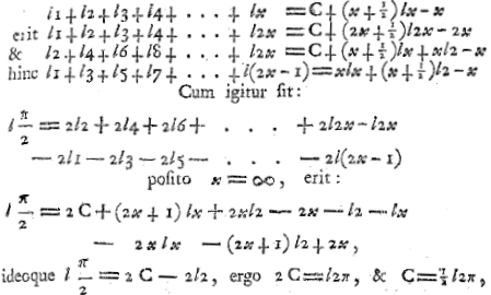
Figure 1.14: Euler and Stirling’s Constant

Taken from [E212]. Euler uses the Wallis product formula for $\pi$ to find the Stirling constant, $\log\sqrt{2\pi}$, in the Stirling formula. Euler wrote $l$ for $\log$.

and hence

$$\sum_{k=1}^{2x}\log k=A+\left(2x+\dfrac{1}{2}\right)\log(2x)-2x.$$

Moreover,

$$\sum_{k=1}^{x}\log(2k)=\sum_{k=1}^{x}\log k+\sum_{k=1}^{x}\log 2=x\log 2+A+\left(x+\dfrac{1}{2}\right)\log x-x.$$

Therefore, finally

$$\sum_{k=1}^{x}\log(2k-1)=\sum_{k=1}^{2x}\log k-\sum_{k=1}^{x}\log(2k)=x\log x+\left(x+\dfrac{1}{2}\right)\log 2-x.$$

Now, Euler’s idea also was to use the Wallis product formula for $\pi$, i.e.

$$\dfrac{\pi}{2}=\dfrac{2}{1}\cdot\dfrac{2\cdot 4}{3\cdot 3}\cdot\dfrac{4\cdot 6}{5\cdot 5}\cdot\dfrac{6\cdot 8}{7\cdot 7}\cdot\dfrac{8\cdot 10}{9\cdot 9}\cdot\text{etc.}$$

Therefore,

$$\log\dfrac{\pi}{2}=\lim_{x\rightarrow\infty}\left(2\sum_{k=1}^{x}\log(2k)-\log(2x)-2\sum_{k=1}^{x}\log(2k-1)\right).$$

Thus, combining the corresponding equations and taking the limit, we find

$$\log\dfrac{\pi}{2}=2A-2\log 2$$

and hence

$$A=\log\sqrt{2\pi}.$$

Finally, we can write down our expression for $y(x)=\log\Gamma(x)$ in its final form:

$$\log\Gamma(x)=x\log x-x-\dfrac{1}{2}\log x+\log\sqrt{2\pi}+\sum_{k=1}^{\infty}\dfrac{B_{2m}}{2m(2m-1)x^{2m-1}}.$$

Finally, taking exponentials we arrive at the limit formula. Concerning this formula, we stress here again that this is an asymptotic expansion and thus one rather should write:

$$\log\Gamma(x)\sim x\log x-x-\dfrac{1}{2}\log x+\log\sqrt{2\pi}+\sum_{k=1}^{\infty}\dfrac{B_{2m}}{2m(2m-1)x^{2m-1}}.$$

∎

1.6.5 Generalized Factorials

1.6.5.1 Euler’s Results on generalized factorials

In [E661], as the title Variae considerationes circa series hypergeometricas suggests, Euler studied more general factorials. The generalisation is that the difference equation $f(n+1)=nf(n)$ is now replaced by the slightly more general one $f(n+1)=(a+bn)f(n)$ with positive real numbers $a,b$. Having discussed the moment ansatz, we can easily solve such equations, but Euler had other ideas. He wanted to find Stirling-like formulas and used the Euler-Maclaurin summation formula. Otherwise, the ideas in this paper are not new. Regardless, we want to state his results. He introduced the following functions:

$$\begin{array}[]{lll}\Gamma(i)&\leavevmode\nobreak\ =\nobreak\leavevmode&a(a+b)(a+2b)(a+3b)\cdots(a+(i-1)b)\\ \Delta(i)&\leavevmode\nobreak\ =\nobreak\leavevmode&a(a+2b)(a+4b)\cdots(a+(2i-2)b)\\ \theta(i)&\leavevmode\nobreak\ =\nobreak\leavevmode&(a+b)(a+3b)\cdots(a+(2i-1)b).\end{array}$$

He established several relations among them and found the Stirling-like formulas, i.e. asymptotic expansions,

$$\begin{array}[]{lll}\Gamma(i)&\leavevmode\nobreak\ \sim\nobreak\leavevmode&Ae^{-i}(a-b+bi)^{\frac{a}{b}+i-\frac{1}{2}}\\ \Delta(i)&\leavevmode\nobreak\ \sim\nobreak\leavevmode&Be^{-i}(a-2b+2bi)^{\frac{a}{2b}+i-\frac{1}{2}}\\ \theta(i)&\leavevmode\nobreak\ \sim\nobreak\leavevmode&Ce^{-i}(a-b+2bi)^{\frac{a}{2b}+i}.\end{array}$$

All equations hold only for $i\rightarrow\infty$. In these formulas, $\Gamma(i)$ is not to be confused with our $\Gamma$-function. We simply adopted Euler’s notation from [E661]. Euler could not determine the constants $A$, $B$, $C$ as in the case of Stirling’s formula, since he did not have access to a Wallis-like product and could not argue analogously as we showed in section 1.6.4.1. But we, in possession of all necessary tools, will evaluate these constants in the next sections.

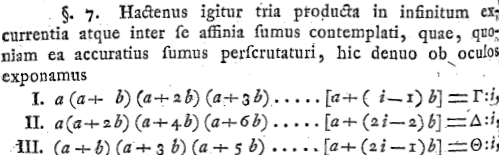
Figure 1.15: Euler’s generalized Factorials

Euler’s definition of the generalized factorials he considered in [E661]. The scan is taken from the same paper.

1.6.5.2 Evaluation of the Constant $A$

We will present the evaluation of the constant $A$ in the first of the three asymptotic expansions. We claim that the following calculations could all have been done by Euler himself, since all steps involved concepts or techniques that he used elsewhere in a similar way. We have:

Theorem 1.6.9.

Let $F$ be a meromorphic function that is logarithmically convex on the positive real axis. Furthermore, let $F$ satisfy:

$$F(x+1)=(a+bx)F(x)\quad\forall\leavevmode\nobreak\ a,b,x>0\quad\text{and}\quad F(1)=1.$$

Then $F$ has the following asymptotic expansion:

$$F(x)\sim A\left(a-b+bx\right)^{\frac{a}{b}-\frac{1}{2}+x}e^{-x}\quad\text{for}\quad x\rightarrow\infty$$

with

$$A=\dfrac{b^{-\frac{a}{b}-\frac{1}{2}}\sqrt{2\pi}e^{1-\frac{a}{b}}}{\Gamma\left(1+\frac{a}{b}\right)}.$$

Proof.

That the general asymptotic formula is correct follows from an application of the Euler-Maclaurin summation formula, which will be discussed in section 1.7, and was already shown by Euler in [E661], as we mentioned above. Thus, we will only determine the constant $A$.
To this end, recall the solution for the propounded difference equation we found in section 1.5.4.4, i.e.

$$F(x)=C\int\limits_{0}^{\infty}t^{x-1+\frac{a}{b}}e^{-\frac{t}{b}}dt\quad\text{for}\quad x-1+\frac{a}{b}>0.$$

$C$ is a constant that we did not need in the previous investigations. But we will determine it here. Before doing so, let us express $F$ in terms of the familiar $\Gamma$-function. Substituting $\frac{t}{b}=y$ in the above integral, we find:

$$F(x)=C\int\limits_{0}^{\infty}b^{x+\frac{a}{b}}y^{x-1+\frac{a}{b}}e^{-y}dy=Cb^{x+\frac{a}{b}}\Gamma\left(x+\dfrac{a}{b}\right),$$

where we used the integral representation of the $\Gamma$-function in the last step. Therefore, from $F(1)=1$:

$$C=\dfrac{b^{-\frac{a}{b}-1}}{\Gamma\left(1+\frac{a}{b}\right)}.$$

Finally, we have to use the Stirling-formula from section 1.6.4.1 yielding the asymptotic expansion of $\Gamma(x+1)$ for large $x$; we just have to replace $x$ by $x+\frac{a}{b}$ in that formula and find the asymptotic expansion:

$$F(x+1)\sim\dfrac{b^{-\frac{a}{b}-1}}{\Gamma\left(1+\frac{a}{b}\right)}b^{x+1+\frac{a}{b}}\sqrt{2\pi}\left(x+\dfrac{a}{b}\right)^{x+\frac{a}{b}+\frac{1}{2}}e^{-x-\frac{a}{b}}\quad\text{for}\quad x\rightarrow\infty$$

Therefore,

$$F(x)\sim\dfrac{b^{-\frac{a}{b}-1}}{\Gamma\left(1+\frac{a}{b}\right)}b^{x+\frac{a}{b}}\sqrt{2\pi}\left(x-1+\dfrac{a}{b}\right)^{x+\frac{a}{b}-\frac{1}{2}}e^{-x-\frac{a}{b}+1}\quad x\rightarrow\infty.$$

Massaging this into a form resembling Euler’s:

$$F(x)\sim\dfrac{b^{-\frac{a}{b}-\frac{1}{2}}}{\Gamma\left(1+\frac{a}{b}\right)}\sqrt{2\pi}\left(bx-b+a\right)^{x+\frac{a}{b}-\frac{1}{2}}e^{-x}\cdot e^{1-\frac{a}{b}}\quad x\rightarrow\infty.$$

Therefore, comparing this to Euler’s result we find:

$$A=\dfrac{\sqrt{2\pi}\cdot e^{1-\frac{a}{b}}}{\Gamma\left(1+\frac{a}{b}\right)}\cdot b^{-\frac{a}{b}-\frac{1}{2}}.$$

∎

1.6.5.3 Finding the other Constants

Having found $A$ in this way, one can proceed analogously to find the others. Concerning the function $\Delta(x)$, satisfying

$$\Delta(x+1)=(a+2bx)\Delta(x),\quad a,b>0\quad\text{with}\quad\Delta(1)=1,$$

we can derive the asymptotic expansion just replacing $b$ by $2b$ in the expansion found for $F$. Hence we find:

$$\Delta(x)\sim\dfrac{(2b)^{-\frac{a}{2b}-\frac{1}{2}}}{\Gamma\left(1+\frac{a}{2b}\right)}\sqrt{2\pi}\left(2bx-2b+a\right)^{x+\frac{a}{2b}-\frac{1}{2}}e^{-x}\cdot e^{1-\frac{a}{2b}}\quad x\rightarrow\infty.$$

Thus, the constant $B$ in Euler’s formulas from section 1.6.5.1 is:

$$B=\dfrac{(2b)^{-\frac{a}{2b}-\frac{1}{2}}}{\Gamma\left(1+\frac{a}{2b}\right)}\sqrt{2\pi}e^{1-\frac{a}{2b}}.$$

Finally, Euler introduced the function $\theta(x)$ satisfying

$$\theta(x+1)=(a+(2b+1)x)\theta(x),\quad a,b>0\quad\text{with}\quad\theta(0)=1.$$

Additionally, it is logarithmically convex, as it follows from Euler’s definition given in 1.6.5.1. Here, one is inclined to derive the asymptotic expansion from the one of $F$ again. But this does not lead to a form resembling Euler’s. To get to such a form, note that

$$\Delta\left(x+\dfrac{1}{2}\right)=k\theta(x)$$

for a constant $k$, since both sides satisfy the same functional equation and are logarithmically convex on the positive real axis. From the special case $x=0$ the constant $k$ is found to be $=\frac{1}{\Delta(\frac{1}{2})}$. Let us evaluate $k$. First, we have:

$$\Delta(x)=\dfrac{(2b)^{-\frac{a}{2b}-1}}{\Gamma\left(1+\frac{a}{2b}\right)}\cdot(2b)^{x+\frac{a}{2b}}\cdot\Gamma\left(x+\dfrac{a}{2b}\right).$$

Hence

$$\Delta\left(\dfrac{1}{2}\right)=(2b)^{-\frac{1}{2}}\cdot\dfrac{\Gamma\left(\frac{1}{2}+\frac{a}{2b}\right)}{\Gamma\left(1+\frac{a}{2b}\right)}.$$

Therefore, we can now use the asymptotic expansion of $\Delta$ to find the one for $\theta:$

$$\theta(x)\sim\dfrac{1}{\Delta\left(\frac{1}{2}\right)}\cdot B(2bx-b+a)^{x+\frac{a}{2b}}e^{-x-\frac{1}{2}}.$$

Thus, the constant $C$ in Euler’s formulas from 1.6.5.1 can be expressed in terms of $k=\frac{1}{\Delta\left(\frac{1}{2}\right)}$ and $B$, which we already found:

$$C=k\cdot Be^{-\frac{1}{2}}$$

1.6.5.4 Euler’s Relations among the Constants

As mentioned in section 1.6.5.1, in $\S 17$ of [E661], Euler also proved some relations among the constants $A$, $B$ and $C$ in the asymptotic expansions. More precisely, he proved:

$$B=\Delta\left(\frac{1}{2}\right)e^{\frac{1}{2}}C\quad\text{and}\quad B=\sqrt{A\Delta\left(\frac{1}{2}\right)e}.$$

The relation among $B$ follows directly from our calculations so that we focus on the derivation of the other one, among $A$ and $B$. To prove it from our explicit formulas for $A$ and $B$, we need the following

Theorem 1.6.10 (Legendre’s duplication formula for $\Gamma$).

The following equation holds for all $z\in\mathbb{C}$:

$$\Gamma(z)\Gamma\left(z+\dfrac{1}{2}\right)=2^{1-2z}\sqrt{\pi}\Gamma(2z).$$

This formula is a special case of the Gaußian multiplication formula for the $\Gamma$-function, which will be discussed in quite some detail below in section LABEL:subsec:_Multiplication_Formula.
But, for now, let us consider $A\cdot\Delta\left(\frac{1}{2}\right)\cdot e$; inserting the values for $A$ and $\Delta\left(\frac{1}{2}\right)$:

$$A\Delta\left(\dfrac{1}{2}\right)\cdot e=\dfrac{b^{-\frac{a}{b}-\frac{1}{2}}\sqrt{2\pi}e^{1-\frac{a}{b}}}{\Gamma\left(1+\frac{a}{b}\right)}\cdot(2b)^{-\frac{1}{2}}\dfrac{\Gamma\left(\frac{1}{2}+\frac{a}{2b}\right)}{\Gamma\left(1+\frac{a}{2b}\right)}\cdot e.$$

Applying Legendre’s duplication formula for $z=\frac{1}{2}+\frac{a}{2b}$, this equation becomes

$$A\Delta\left(\dfrac{1}{2}\right)\cdot e=\dfrac{b^{-\frac{a}{b}-\frac{1}{2}}\sqrt{2\pi}\cdot e^{2-\frac{a}{b}}(2b)^{-\frac{1}{2}}\cdot\sqrt{\pi}\cdot 2^{-\frac{a}{b}}}{\Gamma\left(\frac{1}{2}+\frac{a}{2b}\right)\left(\Gamma\left(1+\frac{a}{2b}\right)\right)^{2}}\Gamma\left(\dfrac{1}{2}+\dfrac{a}{2b}\right).$$

This expression can be simplified to

$$A\Delta\left(\dfrac{1}{2}\right)\cdot e=\dfrac{(2b)^{-\frac{a}{b}-1}\cdot 2\pi\cdot e^{2-\frac{a}{b}}}{\left(\Gamma\left(1+\frac{a}{2b}\right)\right)^{2}}$$

The right-hand side is just $B^{2}$; thus, the relation is proven.
Finally, we want to point out that Euler in [E661] found the relations among $A$, $B$, $C$ from the relations among the functions $\Delta$, $F$ and $\theta$. Therefore, Legendre’s duplication formula for the $\Gamma$-function follows from the relations among $A$, $B$ and $C$. Euler did not notice this, of course. But below in LABEL:subsubsec:_Euler's_Version_of_the_Multiplication_Formula we will show that later in his career Euler found a formula equivalent to the multiplication formula for the $\Gamma$-function containing Legendre’s formula as a special case.

1.7 Solution of $\log\Gamma(x+1)-\log\Gamma(x)=\log x$ via the Euler-Maclaurin Formula

1.7.1 Overview on the Section

We will present Euler’s derivation in section 1.7.2 and the modern derivation of the Euler-Maclaurin summation formula in section 1.7.4. Euler also saw the formula as the solution of the difference equation, i.e., as a tool to calculate finite sums.

1.7.2 Euler’s Derivation of the Formula

Euler derived the Euler-Maclaurin summation formula on various occasions. The first occasion was in 1738 in [E25], but he also gave derivations in 1741 in [E47] and in his book [E212] published 1755.
He saw it as a tool to calculate finite sums and this helps to understand his derivation. For, we already mentioned that

$$f(n):=\sum_{k=1}^{n}g(k)$$

satisfies the functional equation

$$f(n)-f(n-1)=g(n)\quad\forall n\in\mathbb{N}.$$

And the idea to find the function $f$ is still the same as in section 1.6.2 (or in [E189]), i.e. to solve the above difference equation. Using Taylor’s theorem, he wrote

$$f(n-1)=\sum_{k=0}^{\infty}\dfrac{(-1)^{k}f^{(k)}(n)}{k!}.$$

This, as above, led him to a differential equation of infinite order, i.e.

$$\sum_{k=1}^{\infty}\dfrac{(-1)^{k}f^{(k)}(n)}{k!}=g(n).$$

Now, it is important to note that at the time of his first proof in 1738 in [E25] and later in 1741 in [E47], Euler had not developed the theory how to solve differential equations with constant coefficients yet. But Euler had another idea: He made an educated guess. More precisely, he assumed the solution to be of the following form:

$$f(n)=\alpha\int\limits^{n}g(k)dk+\beta\dfrac{dg(n)}{dn}+\gamma\dfrac{d^{2}g(n)}{dn^{2}}+\delta\dfrac{d^{3}g(n)}{dn^{3}}+\varepsilon\dfrac{d^{4}g(n)}{dn^{4}}+\text{etc.}$$

Inserting this ansatz into the differential equation of infinite order gives recursive relations to define the coefficients $\alpha,\beta,\gamma$ etc.

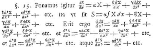
Figure 1.16: Finding the Euler-Maclaurin Summation Formula

Scan taken from [E47]. Euler makes the ansatz with undetermined coefficients $\alpha$, $\beta$, $\gamma$ etc. to solve the differential equation of infinite order (derived from the difference equation $S(x+1)-S(x)=X$) for $S$. In the following paragraphs, he found the recursive relation for the coefficients. This led him to the Euler-Maclaurin summation formula.

In his 1755 book [E212], Euler then also proved that the coefficients are generated by:

$$\dfrac{z}{e^{-z}-1}$$

if it is expanded into a Taylor series around the origin. This is almost the modern definition of the Bernoulli numbers.

Definition 1.7.1 (Bernoulli Numbers).

The Bernoulli numbers are defined via a generating function. More precisely, we define the $n$-th Bernoulli number $B_{n}$ via

$$\dfrac{z}{e^{z}-1}=\sum_{n=0}^{\infty}\dfrac{B_{n}}{n!}z^{n}.$$

Euler calculated many of the Bernoulli numbers, which were defined by Jacob Bernoulli in the context of combinatorics in his 1713 book [Be13], and proved some elementary properties about them, e.g., that all odd Bernoulli numbers except $B_{1}=-\frac{1}{2}$ vanish. He was mainly interested in them, since they appear in his formula for $\zeta(2n)=\frac{1}{1^{2n}}+\frac{1}{2^{2n}}+\frac{1}{3^{2n}}+\cdots$, a connection he realized for the first time in 1750 in [E130]. See also Sandifer’s article in [Br07] (pp. 279 - 303).
Using the Bernoulli numbers, one can write the Euler-Maclaurin formula as

$$f(n+1)=\sum_{k=0}^{n}g(k)=\int\limits^{n}g(k)dk+\sum_{k=0}^{\infty}\dfrac{B_{k+1}}{(k+1)!}\dfrac{d^{k}g(n)}{dn^{k}}.$$

The constant of integration must be determined in such a way that the condition $f(1)=g(0)$ is satisfied. This is at least, how Euler used the formula. The modern formula avoids this problem, essentially by subtracting two sums from each other. Furthermore, we stress that the infinite sum does in general not converge for any value of $n$ and is to be understood as an asymptotic series. We addressed this issue already, when we discussed the Stirling formula 1.6.4.1.

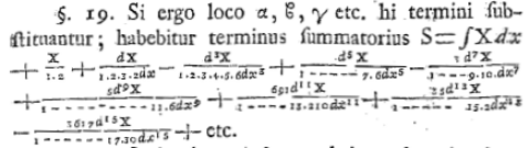
Figure 1.17: The Euler-Maclaurin Sum Formula

Taken from [E47]. Euler states the Euler-Maclaurin formula explicitly for the first time. $\alpha$, $\beta$, $\gamma$ etc. are defined recursively in the same paper. They are the Bernoulli numbers, a fact Euler did not realize at that time.

1.7.2.1 Several Remarks

The derivation of the above series is purely formal and the convergence of the sum is not guaranteed. Indeed, since the Bernoulli numbers increase rapidly (roughly as $(2n)!$, which follows from Euler’s formula for $\zeta(2n)$.), the series actually converges very rarely. Euler was aware of this and only used it for numerical calculations truncating the sum after a certain number of terms. The Euler-Maclaurin summation formula leads to the notion of a semi-convergent series, a term coined by Gauß in 1812 in [Ga28]. $B_{n}$ is small for the first few $n$, whence the series seems to converge taking only a few terms, although the sum if continued to infinity must ultimately diverge, if the derivatives of $g$ do not vanish. An explicit formula for the remainder term, if the sum is truncated at some point, was given by Jacobi in 1834 in [Ja34a] and Poisson.
The issue of semi-convergence troubled Euler and many others, including Gauß in [Ga28]. Nowadays, the right-hand side of the above series is understood as an asymptotic expansion of the sum on the right. We mention [Ha48], [Ba09] and [Va06] again as references discussing the notion of an asymptotic expansion.
Leaving the issues of convergence aside, let us discuss the nature of the formula. Recalling its origin, the solution of a differential equation of infinite order, it has to be a particular solution of that equation. In other words, it has to be a special case of the solution given above in section 1.6. Staying purely formal, it is easier to understand this connection, what we will do in the following section.

1.7.2.2 Purely formal Derivation

We will use the idea that we can replace $\frac{d}{dx}$ by $z$ and an integral by $\frac{1}{z}$ and vice versa. Above we saw that a solution of

$$f(x+1)-f(x)=g(x)$$

is given by

$$f(x)=\dfrac{1}{e^{z}-1}g(x).$$

And next, we expanded $\frac{1}{e^{z}-1}$ into partial fractions and derived the complete solution of the simple difference equation. But we can also expand $\frac{1}{e^{z}-1}$ differently, i.e. into a Laurent series around $z=0$. Using the definition of the Bernoulli numbers above, we find

$$\dfrac{1}{e^{z}-1}=\sum_{n=0}^{\infty}\dfrac{B_{n}}{n!}z^{n-1}=\dfrac{B_{0}}{z}+\sum_{n=0}^{\infty}\dfrac{B_{n+1}}{(n+1)!}z^{n}.$$

Therefore, replacing $\frac{1}{e^{z}-1}$ by the right-hand side of this equation and then replacing $z^{n}$ by $\frac{d^{n}}{dx^{n}}$ and $\frac{1}{z}$ by $\int\limits^{x}$ in the above equation, we have

$$f(x)=B_{0}\int\limits^{x}g(t)dt+\sum_{n=0}^{\infty}\dfrac{B_{n+1}}{(n+1)!}\dfrac{d^{n}g(x)}{dx^{n}}.$$

It is easy to see that this is the Euler-Maclaurin summation formula again. Therefore, the naive and formal derivation easily reproduces both, the general solution and the particular solution provided by the Euler-Maclaurin series, from the general difference equation.

1.7.3 Historical Overview

For the sake of completeness, it will be convenient to give a least a short overview about the results in the theory of differential equations of infinite order. The overview can be subdivided in formal results and rigorously proven results. Naturally, the formal results extend much further, but will we see that the general formulas, derived in purely formal manner, do not hold in every case. And the study of the first rigorous results will reveal, why the the formal approaches are not correct in the most general case.

1.7.3.1 Formal Approaches - From Euler to Bourlet

Although many people contributed to the formal theory of differential equations of infinite order, including Lagrange [La72], Laplace [La20] and many others, the most general result was derived by Bourlet [Bo97] and [Bo99], who basically treated the problem of solving a differential equation as a problem to find the left-inverse operator of the corresponding differential operator as we did in the case of the general difference equation. He wrote $z=\frac{d}{dx}$, and considered the equation

$$F(x,z)f(x)=\sum_{n=0}^{\infty}a_{n}(x)\frac{d^{n}}{dx^{n}}f(x)=g(x),$$

where Bourlet, like Euler, did not specify the functions $a_{n}(x),f(x),g(x)$. Now Bourlet’s simple idea was that, since $F(x,z)$ is an operator, it has (in modern language), a left inverse $X(x,z)$. And treating $z$ as a variable quantity, he derived a partial differential equation that determines $X(x,z)$. It reads as follows:

$$\sum_{n=0}^{\infty}\frac{1}{n!}\frac{\partial^{n}X}{\partial z^{n}}\cdot\frac{\partial^{n}F}{\partial x^{n}}=1.$$

As appealing as this formula might look, it is not true in general. To see this, this consider the equation:

$$\sum_{n=0}^{\infty}\frac{(-x)^{n}}{n!}\frac{d^{n}}{dx^{n}}f(x)=g(x).$$

On the one hand we see, that the left hand side is by Taylor’s theorem equal to:

$$f(0).$$

Thus, $g(x)$ cannot be chosen arbitrarily. On the other hand, Bourlet’s formula would lead to an inverse function, because the corresponding differential equation can be solved. So it gives a solution to an ill-defined question.

1.7.3.2 Rigorous Results - From Carmichel to today

Therefore, formally the theory is established by Bourlet’s formula, a beautiful account of this is given in [Da36], where the main focus is put on solving the equations by mostly formal means. Because of the problems with the formal procedure, mathematicians considered more special problems and considered more special classes of functions, for which rigorous results can be proven. One of the first overview papers on the rigorous results was [Ca36]. Most of the results described in that paper only consider the existence of a solution, but do not give explicit solution formulas. One exception is the theorem we want to quote here.

Theorem 1.7.1.

In the linear differential equation of infinite order

$$a_{0}y+a_{1}y^{\prime}+\cdots=\phi(x)$$

let the constants $a_{\nu}$ be such constants that the function

$$F(z)=a_{0}+a_{1}z+a_{2}z^{2}+\cdots$$

is analytic in the region $|z|\leq q$, i.e. inside a disc, where $q$ is a given positive constant or zero, and let $\phi(x)$ be a function of exponential type not exceeding $q$. If $F(z)$ vanishes at least once in the region $|z|\leq q$, let $n$ be the number of its zeros in this region (each counted according to its multiplicity) and let $P(z)$ be the polynomial of degree $n$ with leading coefficient unity, that $\frac{F(z)}{P(z)}$ does not vanish in the region. If $F(z)$ does not vanish in the region, let $P(z)$ be identically equal to $1$. When $P(z)\equiv 1$, let $P_{n-1}(z)$ be identically equal to zero; otherwise, let it be an arbitrary polynomial of degree $n-1$ (including the case of an arbitrary constant when $n=1$). Then the general solution $y(x)$, subject to the condition that it shall be a function of exponential type not exceeding $q$, may be written in the form

$$y(x)=\frac{1}{2\pi i}\int_{C_{\rho}}\frac{\Psi(s)}{F(s)}ds+\frac{1}{2\pi i}\int_{C_{\rho}}\frac{P_{n-1}(s)}{P_{n}(s)}ds$$

where

$$\Psi(s)=\sum_{\nu=0}^{\infty}\frac{\phi^{(\nu)}(0)}{s^{\nu+1}},$$

and where $C_{\rho}$ is a circle of radius $\rho$ about $0$ as center, $\rho$ being greater than $q$ and such that $F(z)$ is analytic in the region $q>|z|\leq\rho$ and does not vanish there.
If $\phi(x)$ is exactly of exponential type $q$, then the named solution $y(x)$ is also of exponential type $q$.

Having stated this theorem, we see, how carefully it is formulated and that the class of functions is quite restricted. But we have to keep in mind that in the time of this paper, i.e. 1936, the notion and theory of distributions did not exist, making the theorems quite difficult to state. The more recent treatments, e.g., [Du10] start with constructing the appropriate function spaces, before solving any differential equations.

1.7.4 Modern Derivation

It will be illustrative to compare a modern proof of the Euler-Maclaurin summation formula to Euler’s idea. Most modern proofs in modern introductory textbooks are similar. We will present it as it is found in [Koe00] (pp. 223-226). The proof in [Va06] is the same. The proof of the general formula proceeds in several steps, slowly ascending from special cases to the general formula.

1.7.4.1 Euler Maclaurin Formula for $\mathcal{C}^{1}-$functions

We first have to define an auxiliary function

Definition 1.7.2.

We define a function $H:\mathbb{R}\rightarrow\mathbb{R}$ as follows

$$H(x):=\left\{\begin{array}[]{ll}x-[x]-\frac{1}{2}&\quad\text{for}\quad x\in\mathbb{R}\setminus\mathbb{Z}\\ 0&\quad\text{for}\quad x\in\mathbb{Z}\end{array}\right\}$$

$[x]$ is the Gauß bracket of $x$ and expresses the integer part of $x$.

This function obviously has period $1$. Having introduced $H$ in this way, we can state the elementary form of the summation formula

Theorem 1.7.2 (Euler summation formula (simple version)).

Let $f:[1,n]\rightarrow\mathbb{C}$, $n\in\mathbb{N}$ be a once continuously differentiable function, then

$$\sum_{k=1}^{n}f(k)=\int\limits_{1}^{n}f(x)dx+\dfrac{1}{2}(f(1)+f(n))+\int\limits_{1}^{n}H(x)f^{\prime}(x)dx.$$

Proof.

By integration by parts over the interval $[k,k+1]$, one has

$$\int\limits_{k}^{k+1}1\cdot f(x)dx=\left[\left(x-k-\dfrac{1}{2}\right)f(x)\right]_{k}^{k+1}-\int\limits_{k}^{k+1}\left(x-k-\dfrac{1}{2}\right)f^{\prime}(x)dx.$$

Since the function $(x-k-\frac{1}{2})f^{\prime}$ is identical to $Hf^{\prime}$ in the interval $[k;k+1]$, their integrals over the same intervals are identical, thus,

$$\int\limits_{k}^{k+1}1\cdot f(x)dx=\dfrac{1}{2}(f(k+1)-f(k))-\int\limits_{k}^{k+1}H(x)f^{\prime}(x)dx.$$

Summation over $k$ from $1$ to $n-1$ and addition of $\frac{1}{2}(f(1)+f(n))$ then gives the formula. ∎

1.7.4.2 General Euler-Maclaurin Summation Formula

As in the simple case, we need to introduce some auxiliary functions

Definition 1.7.3.

We define functions $H_{k}:\mathbb{R}\rightarrow\mathbb{R}$ recursively as follows:
1) $H_{k}$ is a primitive of $H_{k-1}$, $k\geq 2\in\mathbb{N}$ and $H_{1}:=H$
2) $\int\limits_{0}^{1}H_{k}(x)dx=0$.

Now we can state the general Euler-Maclaurin summation formula

Theorem 1.7.3 (Euler-Maclaurin Summation Formula).

Let $f:[1,n]\rightarrow\mathbb{C}$ be a $\mathcal{C}^{2k+1}$-function and $k\geq 1$. Then we have

$$\sum_{\nu=1}^{n}=\int\limits_{1}^{n}f(x)+\dfrac{1}{2}\left(f(1)+f(n)\right)+\left[\sum_{\kappa=1}^{k}H_{\kappa}(0)f^{(2\kappa-1)}\right]_{1}^{n}+R(f);$$

with

$$R(f)=\int_{1}^{n}H_{2k+1}f^{(2k+1)}dx.$$

Proof.

One just has to note that $H_{k}$ is a periodic function for all $k$, which is seen as follows by induction. We know that $H_{1}=H$ is periodic. Thus, consider

$$H_{k+1}(x+1)-H_{k+1}(x)=\int\limits_{x}^{x+1}H_{k}(t)dt=\int\limits_{0}^{1}H_{k}(t)dt=0,$$

where we used the defining properties of $H_{k}$ and the induction assumption that $H_{k}$ is periodic. Having noticed this, one proceeds just as in the case of the simple Euler-Maclaurin formula, but integrates by parts $2k+1$-times to arrive at the formula.
∎

1.7.4.3 Comparison to Euler’s Idea

First, we want to mention that this idea of the modern proof is basically Jacobi’s, see [Ja34a]. Furthermore, we want to point out that we have in general

$$H_{k}(0)=\dfrac{1}{k!}B_{k}.$$

Thus, Euler’s result and the modern result agree. Anyhow, the modern proof does not obtain the formula from the solution of a difference equation but rather starts from the results and proves it to be correct. In Euler’s case, the formula resulted as an answer to a more general question.
Finally, we used the procedure of iterated integration by parts above in our derivation of the Stirling formula for $n!$ in section 1.6.4.1 and simply ignored $R(f)$ in the calculation. As already mentioned in the same section, this is not justified. A rigorous reasoning requires the theory of asymptotic expansions which we did not want to discuss at that point and hence operated on a formal level. Nevertheless, if understood as an asymptotic expansion, dropping $R(f)$ in the Stirling-formula is justified.

1.8 Interpolation Theory and Difference Calculus

This section mainly discusses chapter 16 and 17 of [E212] and the paper [E613], which Euler stated to be an elaboration of the mentioned chapters.

1.8.1 Overview

Euler again tried to solve the difference equation

$$f(x+1)-f(x)=g(x)$$

in order to find an explicit formula for

$$\sum_{k=1}^{x}g(k-1).$$

The sum, only defined for integer $x$, is interpolated by the solution of the difference equation. But this time, Euler used the rules of difference calculus which he had developed in [E212] to solve the difference equation. Interestingly, addressing issues of convergence, this led him to the concept of Weierstraß products in section LABEL:subsec:_Modern_Idea_-_Weierstrass_product.

1.8.2 Euler’s Idea

Euler’s idea, outlined in [E613], is best explained by an example. Euler tried to find the sum

$$\sum_{k=1}^{x}g(k).$$

This time, he simply added $0$ in a clever way. For, we formally have

$$\begin{array}[]{cccccccccccccccccccccccccc}\sum_{k=1}^{x}g(k)&\leavevmode\nobreak\ =\nobreak\leavevmode&g(1)&\leavevmode\nobreak\ +\nobreak\leavevmode&g(2)&\leavevmode\nobreak\ +\nobreak\leavevmode&g(3)&\leavevmode\nobreak\ +\nobreak\leavevmode&g(4)&\leavevmode\nobreak\ +\nobreak\leavevmode&\text{etc.}\\ &\leavevmode\nobreak\ -\nobreak\leavevmode&g(x+1)&\leavevmode\nobreak\ -\nobreak\leavevmode&g(x+2)&\leavevmode\nobreak\ -\nobreak\leavevmode&g(x+3)&\leavevmode\nobreak\ -\nobreak\leavevmode&g(x+4)&\leavevmode\nobreak\ -\nobreak\leavevmode&\text{etc.}\\ \end{array}$$

Or, in short notation

$$\sum_{k=1}^{x}g(k)=\sum_{k=1}^{\infty}\left(g(k)-g(x+k)\right).$$

As Euler observed, this can only work, if $g(k)-g(x+k)$ converges to zero for $k\rightarrow\infty$.
If the series does not converge, one can again add $0$ in a clever way. If the resulting series does still not converge, one can do it again. Indeed, one can repeat the process arbitrarily often to increase the convergence as much as one wants.
In [E613] Euler divided sums into classes according to the behaviour of their infinitesimal terms. More precisely, the first class contains those series, in which we have $\lim_{k\rightarrow\infty}g(k)=0$. The second class contains those series whose differences of infinitesimal terms vanish, i.e. $\lim_{k\rightarrow\infty}g(x+k+1)-g(x+k)=0$. The third class contains the series, whose second differences vanish etc. From this definition it immediately follows that the series of the $i+1$-th class are a subset of the series of the $i$-th class.
Euler then gave formulas for the first, second and third class and explains how the general formula for the $i-$th class can be constructed. We will only need the first and second class for our discussion. The formula for the first class was stated above. Therefore, we will give the formula for the second class. It reads

$$\begin{array}[]{cccccccccccccccccccccccc}\sum_{k=1}^{x}g(k)&\leavevmode\nobreak\ =\nobreak\leavevmode&(1-x)g(1)&\leavevmode\nobreak\ +\nobreak\leavevmode&(1-x)g(2)&\leavevmode\nobreak\ +\nobreak\leavevmode&(1-x)g(3)&\leavevmode\nobreak\ +\nobreak\leavevmode&\text{etc.}\\ +xg(1)&\leavevmode\nobreak\ +\nobreak\leavevmode&xg(2)&\leavevmode\nobreak\ +\nobreak\leavevmode&xg(3)&\leavevmode\nobreak\ +\nobreak\leavevmode&xg(4)&\leavevmode\nobreak\ +\nobreak\leavevmode&\text{etc.}\\ &\leavevmode\nobreak\ -\nobreak\leavevmode&g(x+1)&\leavevmode\nobreak\ -\nobreak\leavevmode&g(x+2)&\leavevmode\nobreak\ -\nobreak\leavevmode&g(x+3)&\leavevmode\nobreak\ -\nobreak\leavevmode&\text{etc.}\end{array}$$

Or in short notation:

$$\sum_{k=1}^{x}g(k)=xg(1)+\sum_{k=1}^{\infty}\left((1-x)g(k)+xg(k+2)-g(x+k)\right).$$

Whereas the left-hand side only makes sense for integer $x$, this restriction is not necessary on the right-hand side. Therefore, we can interpolate the sum in this way. But let us consider some examples first.

1.8.3 Examples

1.8.3.1 Harmonic Series

Euler chose the harmonic series as his first example, i.e.

$$f(x)=\sum_{k=1}^{x}\dfrac{1}{k}=1+\dfrac{1}{2}+\dfrac{1}{3}+\dfrac{1}{4}+\cdots+\dfrac{1}{x}$$

This series belongs to the first class and hence we can write

$$\begin{array}[]{cccccccccccccc}f(x)&\leavevmode\nobreak\ =\nobreak\leavevmode&\dfrac{1}{1}&\leavevmode\nobreak\ +\nobreak\leavevmode&\dfrac{1}{2}&\leavevmode\nobreak\ +\nobreak\leavevmode&\dfrac{1}{3}&\leavevmode\nobreak\ +\nobreak\leavevmode&\dfrac{1}{4}&\leavevmode\nobreak\ +\nobreak\leavevmode&\text{etc.}\\ &\leavevmode\nobreak\ -\nobreak\leavevmode&\dfrac{1}{x+1}&\leavevmode\nobreak\ -\nobreak\leavevmode&\dfrac{1}{x+2}&\leavevmode\nobreak\ -\nobreak\leavevmode&\dfrac{1}{x+3}&\leavevmode\nobreak\ -\nobreak\leavevmode&\dfrac{1}{x+4}&\leavevmode\nobreak\ -\nobreak\leavevmode&\text{etc.}\\ \end{array}$$

And adding each two terms written above each other, we find:

$$f(x)=\sum_{k=1}^{\infty}\dfrac{x}{k(x+k)}=\dfrac{x}{1(x+1)}+\dfrac{x}{2(x+2)}+\dfrac{x}{3(x+3)}+\dfrac{x}{4(x+4)}+\text{etc.},$$

Trying to find the derivative of the function, in his book [E212], Euler arrived at the Taylor series expansion of this series. For this, he just expanded each term $\frac{x}{k(x+k)}$ into a power series via the geometric series and summed the resulting series columnwise.

1.8.3.2 $\Gamma(x)$-function

But we are mainly interested in the expression for the $\Gamma$-function arising from this idea. Since we have $\Gamma(x+1)=x\Gamma(x)$, we also have $\log\Gamma(x+1)-\log\Gamma(x)=\log x$. Therefore, we can, as we did above, consider $\log\Gamma(x)$ as the solution of the simple difference equation, and for integer $x$ we have

$$\log\Gamma(x+1)=\sum_{k=1}^{x}\log(k).$$

Since $\log(k+1)-\log(k)=\log\left(1+\frac{1}{k}\right)$ tends to zero for infinite $k$, the series belongs to the second class. Applying the corresponding formula, we obtain

$$\begin{array}[]{cccccccccccccccccccccccc}\sum_{k=1}^{x}\log(k)&\leavevmode\nobreak\ =\nobreak\leavevmode&(1-x)\log(1)&\leavevmode\nobreak\ +\nobreak\leavevmode&(1-x)\log(2)&\leavevmode\nobreak\ +\nobreak\leavevmode&(1-x)\log(3)&\leavevmode\nobreak\ +\nobreak\leavevmode&\text{etc.}\\ +x\log(1)&\leavevmode\nobreak\ +\nobreak\leavevmode&x\log(2)&\leavevmode\nobreak\ +\nobreak\leavevmode&x\log(3)&\leavevmode\nobreak\ +\nobreak\leavevmode&x\log(4)&\leavevmode\nobreak\ +\nobreak\leavevmode&\text{etc.}\\ &\leavevmode\nobreak\ -\nobreak\leavevmode&\log(x+1)&\leavevmode\nobreak\ -\nobreak\leavevmode&\log(x+2)&\leavevmode\nobreak\ -\nobreak\leavevmode&\log(x+3)&\leavevmode\nobreak\ -\nobreak\leavevmode&\text{etc.}\end{array}$$

Collecting the columns, we arrive at:

$$\log(\Gamma(x+1))=\log(1^{1-x})+\log\left(\dfrac{1^{1-x}2^{x}}{x+1}\right)+\log\left(\dfrac{2^{1-x}3^{x}}{x+2}\right)+\log\left(\dfrac{3^{1-x}4^{x}}{x+3}\right)+\text{etc.}$$

Taking exponentials, we arrive at Euler’s first formula for $x!$ in [E19].

$$x!=\Gamma(x+1)=1^{1-x}\cdot\dfrac{1^{1-x}2^{x}}{x+1}\cdot\dfrac{2^{1-x}3^{x}}{x+2}\cdot\dfrac{3^{1-x}4^{x}}{x+3}\cdot\text{etc.}=\prod_{k=1}^{\infty}\dfrac{k^{1-x}(k+1)^{x}}{x+k}$$

1.8.4 Difference Calculus according to Euler

Here, we will explain in a bit more detail how Euler arrived at his formulas. To this end, we need to explain his results on difference calculus. He outlined his ideas in his book [E212] and also in [E613]. We want to state and prove his main formula from [E613] for the finite sum of $x$ terms.

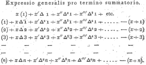
Figure 1.18: Euler’s Key Formula in the Calculus of Differences

Taken from [E613]. Euler’s main formula from the paper. He used the word "summatory" to describe the sum of a series up to $n$ terms and writes $(x)$ to denote the sum from $1$ to $x$. $\Delta^{k}$ denotes the $k$-th difference. Furthermore, Euler did not use a separate letter to denote a function. This is suppressed in his notation, e.g., $(x+3)$ is to be understood a $(f(x+3))$ for a general function $f$.