Immersed boundary simulations of fluid shear-induced deformation of a cantilever beam

Abstract

We derive a mathematical model and the corresponding computational scheme to study deflection of a two-dimensional elastic cantilever beam immersed in a channel, where one end of the beam is fixed to the channel wall. The immersed boundary method has been employed to simulate numerically the fluid-structure interaction problem. We investigate how variations in physical and numerical parameters change the effective material properties of the elastic beam and compare the results qualitatively with linear beam theory. We also pay careful attention to “corner effects” – irregularities in beam shape near the free and fixed ends – and show how this can be remedied by smoothing out the corners with a “fillet” or rounded shape. Finally, we extend the immersed boundary formulation to include porosity in the beam and investigate the effect that the resultant porous flow has on beam deflection.

1 Introduction

In this paper, we derive a mathematical model and the corresponding computational scheme to study the deflection of a two-dimensional deformable elastic cantilever beam in response to a surrounding fluid flow. We will study cantilever beam immersed in a channel flow, where one end of the beam is fixed to the channel wall. We will not impose a given shear flow but rather drive the motion via two walls: one fixed and one moving with constant velocity. In the absence of a beam or other channel obstruction, the flow would develop into a simple linear shear flow (also called Couette flow). We also study the effect of introducing a small porosity into the beam structure, and compare the flow over porous and solid (non-porous) beams. The choice of such a porous cantilever is motivated by our interest in modelling biofilm structures in the near future [1]. A biofilm is a collection of microorganisms (immersed in fluid) that adhere to each other and often also on a nearby surface. Fluid-structure interaction (FSI) plays a key role in several phases of the biofilm life cycle, one being in the deformation of biofilm columns due to fluid forces. We extract from this scenario an idealized 2D model problem in which a rectangular cantilever beam deforms in response to a shear flow. The method we develop may also be useful for simulating other systems arising in applications from biology (e.g., glycocalyx, cilia) and engineering (e.g., MEMS, micropillars).

The study of a cantilever beam is a classical problem in solid mechanics [2] that has been applied in studies of a wide range of applications. These studies include the response of a cantilever to a uniformly distributed or varying load [2] or to a surrounding fluid flow [3, 4, 5, 6, 7]. For example, Pozrikidis [4] studied shear flow over a periodic array of cylindrical rods attached to a substrate in order to determine the macroscopic slip velocity. He also computed the hydrodynamics load exerted along the rod as well as estimating the flow-induced deflection. Shortly afterwards, Pozrikidis [5] studied shear flow past an elastic rod attached to a plane surface (as well as a doubly-periodic array of such rods), motivated by the study of biological flows involving ciliated surfaces. His mathematical framework combined slender-body theory for computing the hydrodynamic load with classical beam theory for computing the rod dynamics. Small vibrations of a thin flexible beam immersed in a laminar flow was studied by Farjoun and Schaeffer [6], where the authors assumed that the dominant restoring force was due to tension caused by shear stress. Goza and Colonius [8] presented a strongly coupled immersed boundary method for FSI problems involving thin deforming bodies. The method was found to be stable for arbitrary choices of solid to fluid mass ratios.

Because we are motivated by the study of problems involving deforming biofilm layers, where the effects of porosity can be important, we will also be investigating the behaviour of porous flexible cantilevers in response to fluid flow. The closest work we have been able to identify regarding porous beams is a mathematical model for an incompressible poro-elastic beam [9] in which the internal porous fluid flow is confined to the axial direction of the deformed beam. Other related studies of poroelastic beams can be found in [7, 10, 9, 11], where again the beam was restricted to be permeable in the axial direction only.

Our modelling approach is based on the immersed boundary or IB method, which has been used in the study of problems in fluid-structure interaction problems from biology in particular, but also in a variety of engineering and other applications (see [12, 13] and references therein). The problem under consideration here involves fluid interacting with rigid 1D structures (channel walls) as well as a 2D deformable region (a beam, which can be either porous or solid). Hence, our problem has a mixture of different solid geometries for which the IB method is an ideal choice [14, 13]. Some researchers have applied the IB method to simulate the dynamics of cilia which individually bear a striking resemblance to a flexible cantilever beam (e.g., [15, 16, 17]). The issue of porous elastic boundaries has also been addressed in the IB context, for example by Kim and Peskin [18] who were the first to incorporate porosity within the IB framework in a study of parachute dynamics. Their approach to handling porous air vents at the apex of the chute was to allow allow the normal velocity of the canopy to differ from that of the fluid by an amount proportional to the normal component of the boundary force. Stockie [19] followed Kim and Peskin’s approach by incorporating porosity directly through Darcy’s law. We extended the ideas in [18, 19] for a 1D porous membrane with pores directed normal to the surface, to handle the case of solid porous 2D region. We then apply this approach to study deformation of a porous rectangular cantilever beam with no restriction on the direction of the pores. For the general situation we consider here, we have not been able to find any other numerical or experimental results with which we can draw direct comparisons.

The organisation of this paper is as follows. We start in Section 2 by defining the problem geometry and list the governing equations. We also define the IB force density that encompasses the influence of the cantilever beam and bounding walls on the flow. In Section 3 we perform numerical simulations of an elastic, cantilever beam and compare the results to experimental and analytical results available in the literature. Finally, in Section 4, we modify the governing equations to introduce porosity into the beam and compare the results from numerical simulations to the non-porous case.

2 Immersed boundary method

The term “immersed boundary method” is commonly used in the literature to refer not only to a numerical method but also to the underlying mathematical formulation [13]. In this work, we only list the governing equations. The details of the governing equations as well as the numerical algorithm has been discussed in [20, 21].

2.1 Governing equations

The IB formulation consists of a coupled system of nonlinear integro-differential equations that describe both the force generated by a solid, deformable, elastic body and the dynamics of a surrounding incompressible, Newtonian fluid. The method is capable of handling immersed boundaries with a very general shape and configuration, although this study has been restricted to the 2D geometry pictured in Figure 1 wherein an initially rectangular cantilever beam is placed inside a fluid-filled channel. The channel is embedded inside a larger, rectangular fluid domain $\Omega=[0,L_{x}]\times[0,L_{y}]$ and is represented by two horizontal walls. For simplicity, we impose periodic boundary conditions in both the $x$- and $y$-directions of the fluid domain, and the top and bottom channel walls are horizontal lines separated a small distance $h$ from the top and bottom domain boundaries respectively. The lower channel wall $\Gamma^{w1}$ is fixed in space along $y=h$, while the upper wall $\Gamma^{w2}$ lies along $y=L_{y}-h$ and moves to the right with a given constant horizontal speed $u_{\text{\emph{top}}}>0$. In the absence of obstructions in the channel, this setup would generate a horizontal linear shear flow with shear rate $\gamma=u_{\text{\emph{top}}}/(L_{y}-2h)$.

The deformable cantilever beam $\Gamma^{b}$ is initially a rectangle with thickness $W_{b}$ and length $H_{b}$, and has its lower end fixed to the center of the bottom wall. Note that the channel walls $\Gamma^{w1}$ and $\Gamma^{w2}$ are taken to be idealized one-dimensional structures of zero thickness, while the beam is treated as a solid elastic structure, with a well-defined thickness. The details regarding the specification of the geometry and forces on the walls and beam are delayed until Section 2.2.

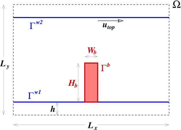
Figure 1: A general elastic boundary $\Gamma=\mathop{\bigcup}_{i=1}^{3}\Gamma^{i}$ that consists of several possibly disconnected components is immersed within a doubly-periodic rectangular fluid domain $\Omega$.

The governing equations for this problem are:

• The motion of the fluid is governed by incompressible Navier-Stokes equations. The variables involved are: $\boldsymbol{u}$ [$\mathrm{cm/s}$](fluid velocity), $p$ [$\mathrm{g/cm\,s^{2}}$](pressure), $\rho$ [$\mathrm{g/cm^{3}}$] (density), $\mu$ [$\mathrm{g/cm\,s}$](dynamic viscosity), $\boldsymbol{f}_{\mbox{}\!\text{\scriptsize\emph{IB}}}(\boldsymbol{q},t)$ [$\mathrm{g/s^{2}}$] ( IB forcing term which captures the effect of the immersed elastic structure on the surrounding fluid)

  $$\rho\frac{\partial\boldsymbol{u}}{\partial t}+\rho\boldsymbol{u}\cdot\nabla\boldsymbol{u}=\mu\nabla^{2}\boldsymbol{u}-\nabla p+\boldsymbol{f}_{\mbox{}\!\text{\scriptsize\emph{IB}}},$$ (1)

  $$\nabla\cdot\boldsymbol{u}=0.$$ (2)

• IB forcing term is calculated by the following equation:

  $$\boldsymbol{f}_{\mbox{}\!\text{\scriptsize\emph{IB}}}(\boldsymbol{x},t)=\int_{\Gamma}\boldsymbol{F}_{\mbox{}\!\text{\scriptsize\emph{IB}}}(\boldsymbol{q},t)\,\delta(\boldsymbol{x}-\boldsymbol{X}(\boldsymbol{q},t))\,d\boldsymbol{q},$$ (3)

  The variables involved are: $\boldsymbol{F}_{\mbox{}\!\text{\scriptsize\emph{IB}}}(\boldsymbol{q},t)$ $[\mbox{$\mathrm{g/s^{2}}$}]$(elastic force density) , $\Gamma$ (immersed structure),$\boldsymbol{X}(\boldsymbol{q},t)$ ($\boldsymbol{X}$ [$\mathrm{cm}$])describes the location of the immersed structure and $\boldsymbol{q}$ represents dimensionless parameterization of points on $\Gamma$ ), $\boldsymbol{x}=(x,y)$ [$\mathrm{cm}$]( Fluid domain $\Omega$’s Eulerian coordinates), $\delta(\boldsymbol{x})=\delta(x)\delta(y)$ ( 2D dirac delta function represented by cartesian product of two 1D dirac delta function).

• The motion of the immersed structure is given by the following fibre evolution equation:

  $$\frac{\partial\boldsymbol{X}}{\partial t}=\boldsymbol{u}(\boldsymbol{X}(\boldsymbol{q},t),t)=\int_{\Omega}\boldsymbol{u}(\boldsymbol{x},t)\,\delta(\boldsymbol{x}-\boldsymbol{X}(\boldsymbol{q},t))\,d\boldsymbol{x},$$ (4)

  The discrete version of the above equations are discussed in [20, 21]. In the next section, we discuss the discrete version of $\boldsymbol{F}_{\mbox{}\!\text{\scriptsize\emph{IB}}}$.

2.2 Discrete specification of the IB force density

We next specify the elastic IB forces that are generated by the channel walls and cantilever beam pictured in Figure 1. Keep in mind that because of the two-dimensional geometry, the equivalent three-dimensional flow can be envisioned as extending to infinity in both directions perpendicular to the $x,y$–plane, and hence the walls are actually horizontal planar surfaces whereas the beam behaves as an infinite cantilever plate. We separate the IB force density $\boldsymbol{F}_{\mbox{}\!\text{\scriptsize\emph{IB}}}$ into the sum of three terms, $\boldsymbol{F}_{\mbox{}\!\text{\scriptsize\emph{IB}}}=\boldsymbol{F}^{w}+\boldsymbol{F}^{b}+\boldsymbol{F}^{a}$, where $\boldsymbol{F}^{w}$ represents the force generated by the channel walls, $\boldsymbol{F}^{b}$ is that generated by the beam, and $\boldsymbol{F}^{a}$ derives from the attachment force between the wall and the bottom edge of the beam. Each of these forces is developed separately in the following three sections.

2.2.1 Force density for channel walls, $\boldsymbol{F}^{w}$

Each horizontal wall is discretized using a sequence of IB points that are equally spaced in the fiber parameter $s$. For example, along the stationary bottom wall we define the initial wall point positions by $\boldsymbol{X}^{w1}_{\ell}=\left(\ell h_{w},h\right)$, where $h_{w}=L_{x}/N_{w}$ and $\ell=1,2,\dots,N_{w}$. In the IB framework, the wall is actually permitted to deviate slightly from its target configuration by connecting each wall point to a fixed “tether point” (initially at the same location) using a very stiff spring that exerts a force of the form

$$\boldsymbol{F}^{w1}_{\ell}=\sigma_{w}(\boldsymbol{X}^{w1}_{\ell}-\boldsymbol{X}_{\ell}),$$ (5)

where $\sigma_{w}$ [$\mathrm{g/cm\,s^{2}}$] is the wall spring stiffness and $\boldsymbol{X}_{\ell}$ is the location of the moving IB point. Any deviation of the wall point from corresponding the tether point location generates a force that brings the IB point back towards the tether point, so if the value of $\sigma_{w}$ is large then the wall points can be treated as rigid structure. The tether points do not generate any force but only serve to determine target locations for the moving IB points.

The given horizontal velocity of the top wall points is easily incorporated in the above framework by simply specifying a given motion for the tether points, so that the IB force density becomes

$$\boldsymbol{F}^{w2}_{\ell}=\sigma_{w}(\boldsymbol{X}^{w2}_{\ell}(t)-\boldsymbol{X}_{\ell}),$$ (6)

where $\boldsymbol{X}^{w2}_{\ell}(t)=\big{(}\operatorname{mod}\left(\ell h_{w}+u_{\text{\emph{top}}}t,L_{x}\big{)},L_{y}-h\right)$ and the “modulo $L_{x}$” operation enforces the periodic boundary conditions in $x$. The total force density generated by the two channel walls may then be written as

$$\boldsymbol{F}^{w}=\sum_{\ell=1}^{N_{w}}(\boldsymbol{F}^{w2}_{\ell}+\boldsymbol{F}^{w1}_{\ell}).$$ (7)

2.2.2 Force density for cantilever beam, $\boldsymbol{F}^{b}$

The cantilever beam is discretized using a collection of $N_{b}$ Lagrangian points that lie on its circumference as well as distributed throughout the interior of the beam. We employ the unstructured triangular mesh generator DistMesh [22] (implemented in Matlab) to generate an approximately uniform triangulation for the beam such as that depicted in Figure 2a. The nodes of the triangulation are the IB points $\boldsymbol{X}_{\ell}$, for $\ell=1,2,\dots,N_{b}$ and a network of springs is defined by the edges of the triangles that acts to maintain the shape of the beam.

(a) Rectangular beam		(b) Smoothed beam
(731 points, 1304 triangles)		(743 points, 1320 triangles)

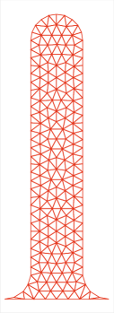
Figure 2: Unstructured triangular mesh for the two beam shapes, generated by distmesh2d. Both have the same height and width, and the fillets for the smoothed beam are constructed in such a way that the areas of the two shapes are equal.

We generate the triangulation using the function distmesh2d with the “scaled edge length function” huniform, which is a built-in function that aims to find a mesh that is as uniform as possible. The “initial edge length” parameter has been assigned equal to $\min(h_{x},h_{y})/3$, which ensures that in practice the mesh satisfies the following constraint

$$\max_{k,\ell}|\boldsymbol{X}_{k}-\boldsymbol{X}_{\ell}|<\frac{1}{2}\,\min(h_{x},h_{y}),$$ (8)

and hence prevents leakage of fluid through the IB that can occur if IB points become too widely separated [13]. We will also perform numerical simulations on the “smoothed beam” shape shown in Figure 2b, where the rectangular corners are replaced by fillets or chamfers – the reasons for the choice of this smoothed shape will be explained later in Section 3.4.

We have defined the spring forces acting on the network, based on the model of Alpkvist and Klapper for viscoelastic biofilm structures [1]. The vector joining two IB points labeled $\ell$ and $m$ is denoted by $\boldsymbol{d}_{\ell,m}(t)=\boldsymbol{X}_{\ell}(t)-\boldsymbol{X}_{m}(t)$ , and the corresponding distance by $d_{\ell,m}(t)=|\boldsymbol{d}_{\ell,m}(t)|$. The network of springs is initially assumed to be in equilibrium (i.e., all spring forces are in balance) so that resting length of each spring is equal to its initial length $d_{\ell,m}(0)$. An incidence matrix whose entries $\mathbb{I}_{\ell,m}$ are either 1 or 0 depending on whether or not the IB points labelled $\ell$ and $m$ are connected to each other is represented by $\mathbb{I}$. Then the net force density acting on the $\ell^{th}$ IB point in the network is given by

$$\boldsymbol{F}^{b}_{\ell}=\sum_{m=1}^{N_{b}}\sigma_{b}\mathbb{I}_{\ell,m}\frac{\boldsymbol{d}_{\ell,m}}{d_{\ell,m}}(d_{\ell,m}(0)-d_{\ell,m}),$$ (9)

where the summation is done over those nodes m of the network for which $\boldsymbol{X}_{m}$ is connected to $\boldsymbol{X}_{\ell}$. The spring stiffness $\sigma_{b}$ [$\mathrm{g/cm\,s^{2}}$] is assumed to be constant for all network connections. The total elastic force density will be generated by all IB points of the beam and will be represented by the expression:

$$\boldsymbol{F}^{b}=\sum_{\ell=1}^{N_{b}}\boldsymbol{F}^{b}_{\ell}.$$ (10)

2.2.3 Force density for attachment between beam and bottom wall, $\boldsymbol{F}^{a}$

In order to hold the lower end of the cantilever beam stationary and coincident with the channel wall, we impose an additional attachment force that connects the points at the base of the beam to the fixed tether points on the bottom wall. The wall and beam points are initially collocated and each pair of points is connected by a very stiff spring. Denote by ${\cal A}$ the attachment point index set which consists of all pairs of IB point indices $(\ell,m)$ for which $\ell$ corresponds to the bottom wall tether point that is linked to the beam IB point $m$. Then the force density arising from the spring joining these two points is

$$\boldsymbol{F}^{a}_{\ell,m}=-\sigma_{a}\,\boldsymbol{d}_{\ell,m},$$ (11)

where $\boldsymbol{d}_{\ell,m}=\boldsymbol{X}^{w1}_{\ell}-\boldsymbol{X}_{m}(t)$ is the vector connecting the wall tether point with fixed location $\boldsymbol{X}^{w1}_{\ell}$ and the beam point at $\boldsymbol{X}_{m}(t)$. Note that the springs in this case have a zero resting length, so that the IB forces act to keep the point pairs in the same location. The spring constant $\sigma_{a}$ is chosen equal to that of the wall–tether connections so that $\sigma_{a}=\sigma_{w}\gg\sigma_{b}$. The total wall–beam attachment force can then be written as

$$\boldsymbol{F}^{a}=\sum_{(\ell,m)\in{\cal A}}\boldsymbol{F}^{a}_{\ell,m}.$$ (12)

3 Numerical simulations of a solid beam

Our numerical simulations presented in this section consist of a parametric study in which we vary values of the beam spring stiffness $\sigma_{b}$, beam length $H_{b}$, and top wall velocity $u_{\text{\emph{top}}}$, the latter of which is related to shear rate via $\gamma=u_{\text{\emph{top}}}/(L_{y}-2h)$. We start with a “base case” corresponding to a beam having dimensions $H_{b}=0.0077$ and $W_{b}=0.0014$. The fluid domain is a square of size $L_{x}=L_{y}=0.03$, and the channel walls are located a distance $h=0.00328$ from the boundaries, which means that the channel width is $L_{y}-2h=0.0234$. This choice of geometry is motivated by one of the test cases considered by Alpkvist and Klapper in [1], and yields a beam aspect ratio $H_{b}/W_{b}\approx 5$ that is large enough to satisfy the thin-beam assumption in the linear theory. This beam length is also small enough (roughly one-third of the channel width) that it doesn’t significantly hinder the bulk flow through the channel. The base value for the top wall velocity is $u_{\text{\emph{top}}}=0.02$, while the spring stiffness values are $\sigma_{b}=560$ and $\sigma_{w}=\sigma_{a}=1000$. For the numerical discretization, we take a fluid grid with $N_{x}=N_{y}=64$ grid points in each direction, and choose $N_{b}=731$ and $N_{w}=210$ in order to satisfy the constraint (8) on the spacing between IB points for the beam and walls. The base case values of all parameters are summarized in Table 1.

As parameters are varied from the base case, we focus on the deflection of the beam from its vertical stress-free state and also the changes in the flow structure. In all cases, the fluid velocity is initialized to zero and the speed of the top wall is ramped up linearly from 0 to $u_{\text{\emph{top}}}$ over the time interval $[0,0.5]$. As the fluid within the channel accelerates and begins to move toward the right, the beam responds by bending downward and to the right as pictured in Figure 3. Because the beam is solid, the flow deflects around the beam, generating a fairly complex flow structure that features recirculation zones in the area near the bottom wall (refer to the streamline patterns in Figure 3a). The beam continues to deform in response to the flow until an equilibrium is attained in which the fluid force acting on the beam and the elastic bending force from the deformed beam are equal. A typical computation requires on the order of 5 to 10 $\mathrm{s}$ for the beam to reach its steady state.

(a)		(b)

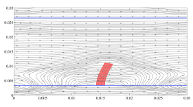
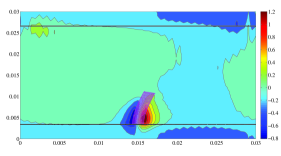
Figure 3: Flow streamlines (left) and pressure contours (right) for the base case simulation at steady state.

We remark that during the course of these rectangular beam simulations, especially for cases with large deflection, we sometimes observe large non-physical irregularities in the shape of the beam in the vicinity of the free end and the attachment at the lower wall especially at high shear rates. For this reason, we also perform a series of simulations with a smoothed beam shape for which the corners at the free end and the beam–wall anchor points are rounded using a fillet or chamfer (refer to Fig. 2b). These results are presented in Section 3.5, and we will see that they exhibit more reasonable deformations near the corners.

Parameter	Description	Value	Units
$L_{x}$	Domain width	0.03	$\mathrm{cm}$
$L_{y}$	Domain height	0.03	$\mathrm{cm}$
$h$	Wall separation distance	0.0033	$\mathrm{cm}$
$H_{b}$	Beam length	0.0077	$\mathrm{cm}$
$W_{b}$	Beam width	0.0014	$\mathrm{cm}$
$\sigma_{b}$	Beam spring stiffness	560	$\mathrm{g/cm\,s^{2}}$
$\sigma_{w}$	Wall spring stiffness	1000	$\mathrm{g/cm\,s^{2}}$
$\sigma_{a}$	Attachment spring stiffness	1000	$\mathrm{g/cm\,s^{2}}$
$u_{\text{\emph{top}}}$	Top wall velocity	0.02	$\mathrm{cm/s}$
$\rho$	Water density	1.0	$\mathrm{g/cm^{3}}$
$\mu$	Water viscosity	0.01	$\mathrm{g/cm\,s}$
Re	Reynolds number $=\rho u_{\text{\emph{top}}}H_{b}/\mu$	0.0154
$N_{x}$, $N_{y}$	Number of fluid grid points	64
$N_{b}$	Number of beam IB points	731
$N_{w}$	Number of wall IB points	210
$\Delta t$	Time step	$10^{-5}$	$\mathrm{s}$

Table 1: “Base case” parameter values for the solid elastic beam problem.

3.1 Euler-Bernoulli beam theory

Before reporting the results of our numerical simulations, we briefly summarize some key results from the Euler-Bernoulli beam theory that pertain to small deflections of a thin cantilever beam. In this case the steady-state configuration of the beam can be desribed by a fourth-order ordinary differential equation [2]

$$EI\frac{d^{4}\xi}{dy^{4}}=q,$$ (13)

where $\xi(y)$ is the horizontal deflection from the vertical equilibrium state at location $y$ along the beam, and $q(y)$ is a given load distribution (in units of force per unit length, $\mathrm{dyne/cm}$ or $\mathrm{g/s^{2}}$). The parameter $EI$ is the flexural rigidity of the beam, which is the product of the Young’s modulus $E$ [$\mathrm{g/cm\,s^{2}}$] and the second moment of area $I$ [$\mathrm{cm^{4}}$]. The linear theory is derived based on the assumptions that the beam is very thin ($W_{b}\ll H_{b}$) and that the deflection $d$ is small relative to the length of the beam ($d/H_{b}\ll 1$).

In particular, we list well-known analytical solutions for the maximum (tip) deflection of the beam in response to two types of applied load: (a) a constant load $q_{0}$ [$\mathrm{dyne/cm}$] distributed across the entire length of the beam : $\displaystyle d=\frac{q_{0}H_{b}^{4}}{8EI}$ and (b) a linearly-varying load that decreases from a maximum $q_{0}$ at the wall to zero at the tip :$\displaystyle d=\frac{q_{0}H_{b}^{4}}{30EI}$ . The tip deflection in all two cases varies according to $d\propto H_{b}^{m}/EI$, with exponent $m=4$. These expressions will be compared qualitatively to the simulated deflections in Section 3.2.

3.2 Dependence of deflection on IB spring stiffness, $\sigma_{b}$

We begin by investigating the effect of changing the spring stiffness $\sigma_{b}$ for links in the beam triangulation, which in turn determines the effective flexural rigidity of the overall beam structure. We note that the beam dimensions $H_{b}=0.0077$ and $W_{b}=0.0014$ corresponding to an aspect ratio of $H_{b}/W_{b}\approx 5$, which is consistent with the thin beam assumption in the linear theory.

Figure 4a depicts the time evolution of the beam tip deflection for values of $\sigma_{b}=140,280,560,1120$, where deflection $d$ is measured in the $x$-direction from the vertical equilibrium configuration. The steady-state deflection values vary from roughly 10% of the beam length for the stiffest beam up to 65% for the smallest value of $\sigma_{b}=70$. It seems reasonable therefore to expect that the larger $\sigma_{b}$ simulations will fall within the small deflection regime, while the smaller $\sigma_{b}$ results might not. Nonetheless, all curves exhibit a similar qualitative behaviour in that the shear flow bends the beam away toward the right and then gradually equilibrates at some maximum deflection. As expected, the stiffer beams have a smaller deflection and also reach their equilibrium state over a shorter time period.

(a) Deflection versus time.

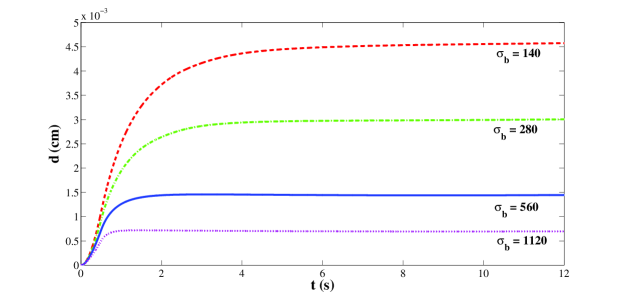
(b) Final deflection versus $\sigma_{b}$.

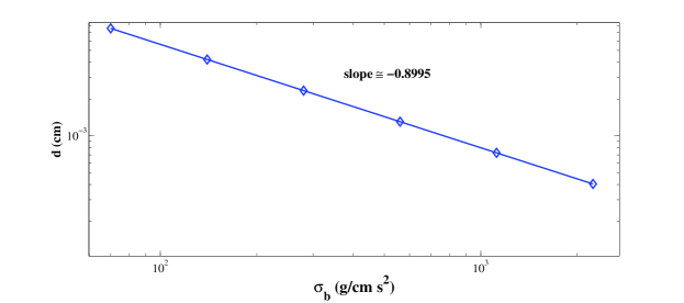
Figure 4: Deflection of the solid cantilever beam as $\sigma_{b}$ is varied, with $H_{b}=0.0077$ and $u_{\text{\emph{top}}}=0.02$. (a) Tip deflection versus time corresponding to $\sigma_{b}\in[70,2240]$. (b) The final (steady-state) tip deflection is plotted against $\sigma_{b}$ with diamond points ($\diamond$) on top of which is superimposed a solid line corresponding to the linear least squares fit (normalized RMS error $=$ 0.055).

Figure 4b plots the steady-state deflection $d$ for all simulations versus $\sigma_{b}$, along with a number of additional results for $\sigma_{b}$ in the interval $[70,2240]$ that fill out the range. The data points are approximated very well by a straight line on a log–log scale; indeed, a least squares fit yields a line with with slope $=-0.8995$ which suggests that the deflection is roughly inversely proportional to $\sigma_{b}$. We can compare these results to the linear beam theory in Section 3.1 which predicts that the deflection is inversely proportional to the flexural rigidity, $EI$, where $E$ is Young’s modulus, $I$ is the area moment of inertia. Assuming that the linear theory holds here (thin beam, small deflection) our computational results suggest that the effective flexural rigidity of our triangulated spring link structure is directly proportional to the spring stiffness, or in other words that $EI\propto\sigma_{b}$.

3.3 Dependence of deflection on beam length, $H_{b}$

Next we perform simulations with different values of the beam length $H_{b}=0.0056$, 0.007, 0.0077, 0.0084, 0.0098, 0.014 (corresponding to aspect ratios of $H_{b}/W_{b}=4$, 5, 5.5, 6, 7, 10 respectively) while holding $\sigma_{b}=560$ and $u_{\text{\emph{top}}}=0.02$ constant. The computed results in Figure 5 show that the tip deflection $d$ increases with $H_{b}$, which is to be expected since a longer beam is clearly more flexible. Furthermore, the dependence of $d$ on $H_{b}$ is again roughly linear on a log-log scale which denotes a power law relationship, and a least squares fit suggests that $d\propto H_{b}^{3.8094}$. This power law exponent is very close to the value 4 predicted by the linear beam theory for the cases when the load force is constant or linearly-varying along the length.

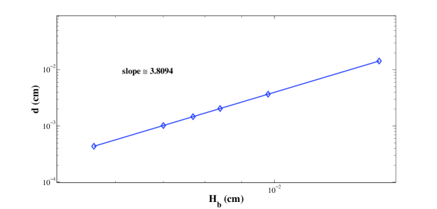
Figure 5: Plot of $H_{b}$ and final deflection $d$ for the non-porous cantilever. Parameters: $\sigma_{b}=560\;\mbox{$\mathrm{g/cm\,s^{2}}$}$, $u_{\text{\emph{top}}}=0.02\;\mbox{$\mathrm{cm/s}$}$. Computed results are shown using diamond points ($\diamond$) on top of which is superimposed a solid line corresponding to the linear least squares fit (normalized RMS error $=$ 0.0432).

3.4 Dependence of deflection on shear velocity, $u_{\text{\emph{top}}}$

In our final sensitivity study, we vary the hydrodynamic force acting on the beam by changing the top wall velocity $u_{\text{\emph{top}}}$. In contrast with the previous cases, we consider much stronger shear flows corresponding to $u_{\text{\emph{top}}}$ values taken from the interval $[0.003,0.6]$, which at the upper end generates beam deformations that are well outside the linear regime. Figure 6 depicts the deformed beam and corresponding streamlines for values of $u_{\text{\emph{top}}}=0.003,0.01,0.02,0.04$, computed over long enough times ($t\approx 25$s) that the beam has essentially reached a steady state configuration.

(a) $u_{\text{\emph{top}}}=0.003$
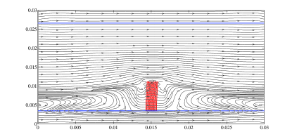
(b) $u_{\text{\emph{top}}}=0.01$
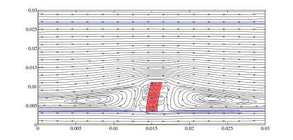
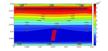
(c) $u_{\text{\emph{top}}}=0.02$ (base case)
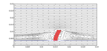
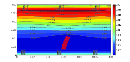
(d) $u_{\text{\emph{top}}}=0.04$

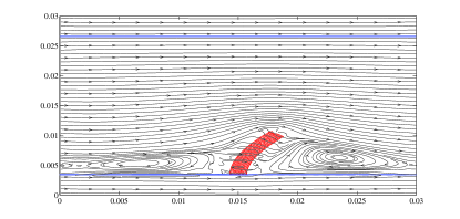
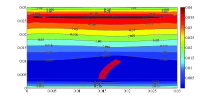
Figure 6: Deflected beam for several values of $u_{\text{\emph{top}}}$, showing streamlines (left) and contours of velocity magnitude (right). Other parameter values are $H_{b}=0.0077\;\mbox{$\mathrm{cm}$}$, $\sigma_{b}=560\;\mbox{$\mathrm{g/cm\,s^{2}}$}$.

If we consider the value of the last streamline lying above the beam tip (from Figure 6), which yields the following values of $\|u\|$:

$\|u\|$	$u_{\text{\emph{top}}}$	$\|u\|/u_{\text{\emph{top}}}$
0.0005	0.003	0.17
0.001	0.01	0.1
0.002	0.02	0.1
0.005	0.04	0.125

Consider the ratio of $\|u\|/u_{\text{\emph{top}}}$ which is approximately 0.1 for all cases, suggesting a clear separation into a boundary layer region where the velocity drops roughly below 10% of the top wall speed.

In each case, the flow separates roughly into two regions: a slow inner flow near the wall that “stalls” ahead of and behind the beam; and a much faster outer shear flow that bypasses the beam. As the outer shear flow increases in strength for higher $u_{\text{\emph{top}}}$, the flow is characterized by recirculating eddies ahead of and behind the beam. We remark also that streamlines pass through the beam and the wall, which at first seems counter-intuitive if the immersed boundaries (and the adjacent fluid) are supposed to be stationary at equilibrium. However, it is important to keep in mind that the IB points making up both the wall and beam experience very small-amplitude oscillations even when the flow is near steady state, and so there are still small non-zero velocities in the neighbourhood of the immersed boundaries.

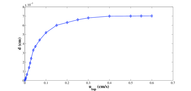
Figure 7: Maximum tip deflection as a function of $u_{\text{\emph{top}}}$ for the solid beam, with parameters $H_{b}=0.0077\;\mbox{$\mathrm{cm}$}$ and $\sigma_{b}=560\;\mbox{$\mathrm{g/cm\,s^{2}}$}$.

The results of these simulations, as well as for a number of other flow speeds, are summarized in Figure 7 on a plot of tip deflection versus top wall velocity, which clearly shows that the beam deformation can be divided into three regimes according to $u_{\text{\emph{top}}}$:

• For $u_{\text{\emph{top}}}\lessapprox 0.03$ or $\gamma\lessapprox 1.282$, the beam deflection is small enough that the linear beam theory applies and the load force varies roughly linearly with $u_{\text{\emph{top}}}$.

• For $u_{\text{\emph{top}}}\gtrapprox 0.12$ or $\gamma\gtrapprox 5.128$, the beam has reached the maximum allowable deflection beyond which any additional increase in $u_{\text{\emph{top}}}$ has little effect on the shape of the beam at steady-state. This behaviour can be attributed to the fact that at larger values of the shear rate, the beam undergoes a significant vertical deflection as it bends downward and to the right, to the point where a large fraction of the beam is oriented parallel to the bulk flow. This in turn reduces the net fluid load force acting on the beam to the point where increasing $u_{\text{\emph{top}}}$ any further does not change the deflection (refer to Figure 6d).

• For intermediate values of $0.03\lessapprox u_{\text{\emph{top}}}\lessapprox 0.12$ or $1.282\lessapprox\gamma\lessapprox 5.128$, the beam is in a transitional state between the low and high shear regimes described above.

Another feature of the beam deformations that becomes evident at higher $u_{\text{\emph{top}}}$ is a large deviation from the original rectangular shape for the IB points near either end of the beam, most notably at the corners. This behaviour is emphasized in Figure 8 which shows two zoomed-in plots of the corner regions near the upper and lower ends of the beam. Near the wall (in the area denoted as region A) large bending forces are generated that cause the beam to “bow out” on both sides. Furthermore, there are noticeable “kinks” at both bottom corners involving the left- and right-most IB points immediately adjacent to the lower wall. At the free end of the beam (zoomed in as region B) the left corner undergoes a significant distortion and the corner point protrudes a significant distance out into the flow owing to the very large shear forces experienced in that region. Both of these behaviours seem non-physical and would not be expected in an actual beam with uniform elastic properties. We attribute the anomalous deformations near both ends of the beam to the existence of sharp corners in the rectangular shape, and the purpose of the next section is to investigate a modified beam shape that aims to eliminate these anomalies.

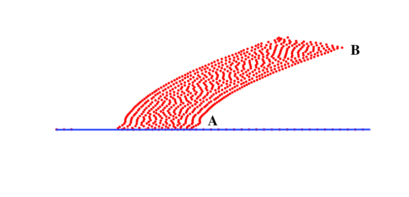
$\nearrow$   B

$\rightarrow$   A

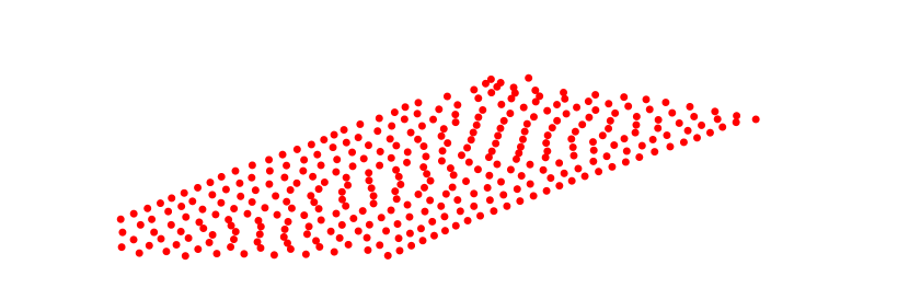
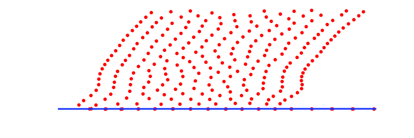
Figure 8: Zoomed view of the large deformations near the corners of the beam when $u_{\text{\emph{top}}}=0.15$.

3.5 Smoothed cantilever beam

We next consider a modified beam shape that has the corners at both ends smoothed out as shown in Figure 2b using using fillets or chamfers. In particular, all four corners have been replaced using circular arcs that have diameter equal to the beam width $W_{b}$. The resulting shape is triangulated as before using distmesh2d, and we choose parameter values that are identical to the $u_{\text{\emph{top}}}=0.15$ simulation from the previous section. The resulting equilibrium beam configuration is depicted in Figure 9, which exhibits a shape that is much more regular than in the rectangular case, even for this high value of the fluid velocity.

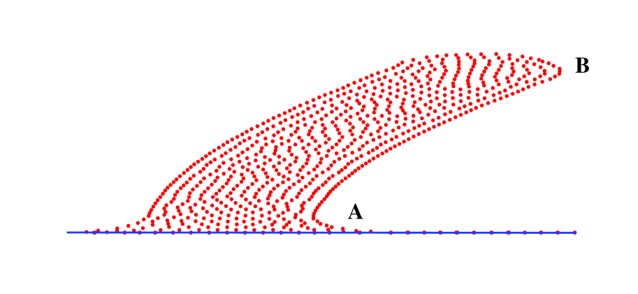
$\nearrow$   B

$\rightarrow$   A

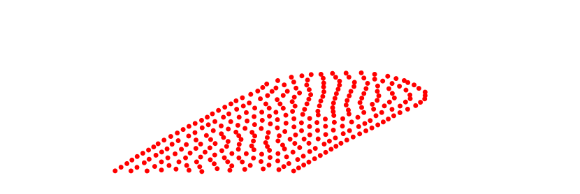
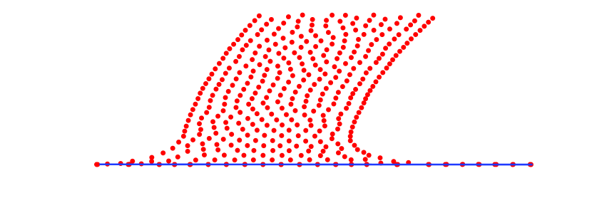
Figure 9: Zoomed view of the two ends of the smoothed beam when $u_{\text{\emph{top}}}=0.15$.

Although the change in beam shape due to smoothing out of the corners does influence the solution, these changes are very small as seen in the two plots of tip deflection versus $u_{\text{\emph{top}}}$ and $\sigma_{b}$ in Figure 10. Indeed, the relative differences between the two solutions is less than 1%. We will therefore employ the smoothed beam shape in all simulations from this point onward. And with a view to applications, the rounded beam shape also has the advantage that it is much more realistic in the context of biofilm problems.

(a)

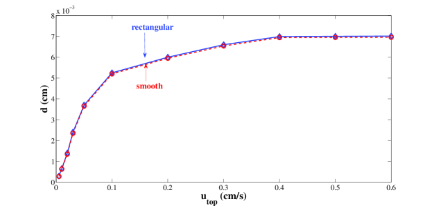
(b)

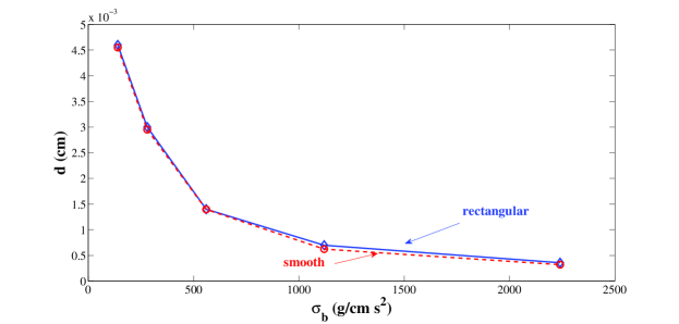
Figure 10: Maximum tip deflection for the rectangular and smooth shapes, plotted as a function of (a) top wall velocity $u_{\text{\emph{top}}}$ and (b) beam spring stiffness $\sigma_{b}$.

4 Numerical simulations of a porous beam

In this section, we consider a porous deformable structure, so that fluid can flow through the structure in response to transmural pressure gradients. Porous structures abound in biological systems, including such examples as artery walls [23] and porous biofilm layers [24, 25, 26, 27]. Porous immersed boundaries also appear in engineering applications such as filtration and separation processes.

Several efforts have been made to generalize the IB method to handle porous structures. The first attempt to incorporate porosity within the IB framework was a study of parachute dynamics by Kim and Peskin [18], wherein the air vents at the apex on the chute were dealt with by allowing the normal velocity of the canopy to differ from that of the fluid by an amount proportional to the normal component of the boundary force (which according to the jump conditions is also proportional to the pressure jump). Stockie [19] built on Kim and Peskin’s approach by incorporating porosity directly using Darcy’s law. The IB method has also been used to study flow through granular media at the pore scale by treating the grains making up the medium as immersed boundaries [15], although the grains themselves are rigid and impermeable in these studies. Layton [28] generalized the closely related immersed interface method by introducing a porous slip velocity in the direction normal to the interface that is driven by differences in both transmural water pressure and solute concentration. In this thesis, we will extend the ideas in [18, 19] for a 1D porous membrane to the case of a solid porous region in 2D. We will use this approach to study the deformation of a porous rectangular cantilever beam, as well as the same smoothed cantilever shape from the previous section.

4.1 Extending the IB formulation to include porosity

The system of equations (1)–(4) is now generalized to include the effect of porosity on the deformable structure. We follow the approaches of Kim and Peskin [18] and Stockie [19] by incorporating a porous slip velocity in the fiber evolution equation. The primary assumption made in [19] and [18] is that all the pores are directed normal to the fiber. The slip velocity is given by $\boldsymbol{u}_{p}=u_{p}\cdot\boldsymbol{t}+v_{p}\cdot\boldsymbol{n}$ where $\boldsymbol{t}$ and $\boldsymbol{n}$ are the unit normal and tangential vectors to the fiber. Due to the assumption just mentioned, the tangential component $v_{p}=0$. For a porous 2D region, it is not realistic to continue with their assumption.

Indeed, we assume a more general porous structure with no restriction in the direction of the pores and fluid can flow in any direction in the porous region. The only way to determine the direction of the fluid velocity is to look at the direction of the pressure gradient, $\nabla p$, that drives the porous flow. In our approach, we also incorporate porous effects via a porous slip velocity $\boldsymbol{u}_{p}$; however here $\boldsymbol{u}_{p}$ is related to the pressure gradient (and not the pressure jump) via Darcy’s law:

$$\boldsymbol{u}_{p}=-\frac{K}{\mu}\nabla p,$$ (14)

where $K$ represents the structure permeability [$cm^{2}$].

The porous beam obeys the same governing equations except that the fiber evolution equation (4) is replaced with

$$\frac{\partial\boldsymbol{X}}{\partial t}=-\boldsymbol{u}_{p}+\int_{\Omega}\boldsymbol{u}(\boldsymbol{x},t)~{}\delta(\boldsymbol{x}-\boldsymbol{X}(s,t))d\boldsymbol{x}.$$ (15)

The negative sign indicates that when the fluid moves through the porous region outward with slip velocity $\boldsymbol{u}_{p}$, the beam in turn moves in the opposite direction, $-\boldsymbol{u}_{p}$.

In our simulations, we have fixed values of $H_{b}=0.0077\;\mbox{$\mathrm{cm}$}$, $\sigma_{b}=560\;\mbox{$\mathrm{g/cm\,s^{2}}$}$ and $u_{\text{\emph{top}}}=0.02\;\mbox{$\mathrm{cm/s}$}$, which corresponds to a shear rate of $0.0855\;\mbox{$\mathrm{s^{-1}}$}$. Permeability $K$ lies in the range $[10^{-10},10^{-4}]\;\mbox{$\mathrm{cm^{2}}$}$ and Figure 11 shows the streamline plots for different values of $K$. It is evident from the figure that for high value of $K$, the fluid passes through the beam without any obstruction but that is not the case for smaller values of $K$. When $K$ is taken as small as $K=10^{-9}$, the flow is almost identical to that for the beam in the non-porous case ($K=0$). Figure 12 shows how the maximum deflection experienced by the cantilever varies with permeability, from which we observe the following:

• For $K\lessapprox 10^{-8}$: the beam is essentially solid and the deflection is the same as in the non-porous case.

• For $10^{-8}\lessapprox K\lessapprox 10^{-6}$: there is a slight increase in maximum deflection. We ascribe this to an increase in porous flow through the beam that acts to enhance the horizontal component of velocity in the region near the beam which in turn increases the shearing force acting on the beam.

• For $K\gtrapprox 10^{-6}$: the porous slip velocity is so large that fluid can pass through the solid structure more freely, hence decreasing the forces acting to deform the beam.

(a) $K=10^{-10}$
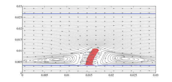
(b) $K=10^{-8}$
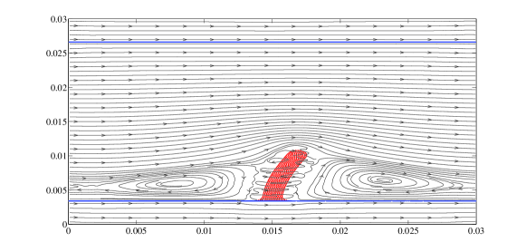
(c) $K=10^{-6}$
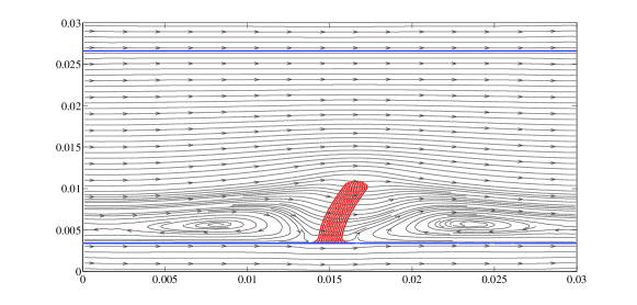
(d) $K=5\times 10^{-5}$

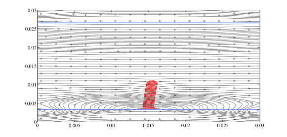
Figure 11: Streamline plots at the point of maximum deflection for a smoothed porous beam with different permeability values.

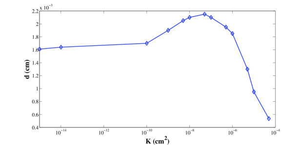
Figure 12: Final deflection ($d$) versus permeability ($K$) for the smoothed porous beam.

5 Conclusions

The main aim of this study was to derive a mathematical model and the corresponding computational scheme to study the deflection of a two-dimensional deformable elastic cantilever beam in response to a surrounding viscous, incompressible fluid flow. The choice of cantilever was motivated by our efforts to model biofilm structures in the near future. Our study included careful validation of the IB approach so that in the future the model can be easily generalized to irregular and highly deformable 3D structures with porosity, detachment etc. We investigated how variations in physical and numerical parameters change the effective material properties of the elastic beam and also made a qualitative comparison of the results with linear beam theory. We also paid attention to “corner effects” (irregularities in beam shape near free end and near wall connection points) and showed how this can be remedied by smoothing out the corners with a filled or round (a standard technique in solid modelling to reduce stress, and in aerodynamics to reduce interference drag). Finally we extended the previous work done on porous IB membranes, by introducing porosity into our deformable elastic beam. In our study we have not imposed any restrictions on the orientation of the pores. The results obtained are consistent with physical intuition. For example, physical intuition suggests that for higher values of permeability, the fluid should pass through the beam without obstruction as compared to smaller values of permeability. The streamline plots obtained in this study also suggests the same. Along the same lines of argument we can say that as permeability of the beam increases, the deflection of the beam should decrease as the force acting to deform the beam decreases and this argument is in good agreement with our numerical results.

In future, we aim to investigate the relationship $EI\propto\sigma_{b}$ by studying two analytical approximations. Our first approach will be by finding a polynomial fit to “typical” computed load, and then deriving the corresponding Euler-Bernoulli beam solution. A second method will apply a simpler spring network and attempt to derive the equilibrium configuration analytically. We will also aim for irregular, deformable shapes corresponding to biofilm columns and streamers. Last but not least, there is a limitation in assuming a 2D geometry and so one of our future aims will be to extend our IB model to 3D cantilevers in the shape of deformed cylinders or parallelipipeds.

References

- [1] E. Alpkvist, I. Klapper, Description of mechanical response including detachment using a novel particle model of biofilm/flow interaction, Water Science and Technology 55 (8-9) (2007) 265–273.
- [2] S. Timoshenko, D. Young, Elements of strength of materials (1968).
- [3] K. Kamrin, C. H. Rycroft, J.-C. Nave, Reference map technique for finite-strain elasticity and fluid–solid interaction, Journal of the Mechanics and Physics of Solids 60 (11) (2012) 1952–1969.
- [4] C. Pozrikidis, Shear flow over cylindrical rods attached to a substrate, Journal of Fluids and Structures 26 (3) (2010) 393–405.
- [5] C. Pozrikidis, Shear flow past slender elastic rods attached to a plane, International Journal of Solids and Structures 48 (1) (2011) 137–143.
- [6] Y. Farjoun, D. G. Schaeffer, A thin cantilever beam in a flow, in: AIP Conference Proceedings, Vol. 1389, 2011, pp. 1446–1449.
- [7] L. P. Li, K. Schulgasser, G. Cederbaum, Theory of poroelastic beams with axial diffusion, Journal of the Mechanics and Physics of Solids 43 (12) (1995) 2023–2042.
- [8] A. Goza, T. Colonius, A strongly-coupled immersed-boundary formulation for thin elastic structures, Journal of Computational Physics 136 (2017) 401–411.
- [9] X. Yang, C. Wang, A nonlinear mathematical model for large deflection of incompressible saturated poroelastic beams, Applied Mathematics and Mechanics (English Edition) 28 (12) (2007) 1587–1595.
- [10] L. P. Li, K. Schulgasser, G. Cederbaum, Large deflection analysis of poroelastic beams, International Journal of Nonlinear Mechanics 33 (1) (1998) 1–14.
- [11] X. Yang, Q. Wen, Dynamic and quasi-static bending of saturated poroelastic timoshenko cantilever beam, Applied Mathematics and Mechanics (English Edition) 31 (8) (2010) 995––1008.
- [12] L. J. Fauci, R. Dillon, Biofluidmechanics of reproduction, Annu. Rev. Fluid Mech. 38 (2006) 371–394.
- [13] C. S. Peskin, The immersed boundary method, Acta numerica 11 (2002) 479–517.
- [14] C. S. Peskin, Flow patterns around heart valves: a numerical method, Journal of computational physics 10 (2) (1972) 252–271.
- [15] R. Dillon, L. Fauci, A microscale model of bacterial and biofilm dynamics in porous media, Biotechnology and Bioengineering 68 (5) (2000) 536–547.
- [16] R. H. Dillon, L. J. Fauci, C. Omoto, X. Yang, Fluid dynamic models of flagellar and ciliary beating, Annals of the New York Academy of Sciences 1101 (1) (2007) 494–505.
- [17] E. A. Schwartz, M. L. Leonard, R. Bizios, S. S. Bowser, Analysis and modeling of the primary cilium bending response to fluid shear, American Journal of Physiology-Renal Physiology 272 (1) (1997) F132–F138.
- [18] Y. Kim, C. S. Peskin, 2–d parachute simulation by the immersed boundary method, SIAM Journal on Scientific Computing 28 (6) (2006) 2294–2312.
- [19] J. M. Stockie, Modelling and simulation of porous immersed boundaries, Computers & Structures 87 (11) (2009) 701–709.
- [20] S. Ghosh, The immersed boundary method for simulating gravitational settling and fluid shear-induced deformation of elastic structures, Ph.D. thesis, Science: Department of Mathematics (2013).
- [21] S. Ghosh, J. M. Stockie, Numerical simulations of particle sedimentation using the immersed boundary method, Communications in Computational Physics 18 (02) (2015) 380–416.
- [22] P. O. Persson, G. Strang, A simple mesh generator in matlab, SIAM review 46 (2) (2004) 329–345.
- [23] Z. J. Huang, J. M. Tarbell, Numerical simulation of mass transfer in porous media of blood vessel walls, American Journal of Physiology-Heart and Circulatory Physiology 273 (1) (1997) H464–H477.
- [24] M. C. M. van Loosdrecht, J. J. Heijnen, H. Eberl, J. Kreft, C. Picioreanu, Mathematical modelling of biofilm structures, Antonie van Leeuwenhoek 81 (2002) 245–256.
- [25] V. T. Nguyen, E. Morgenroth, H. J. Eberl, A mesoscale model for hydrodynamics in biofilms that takes microscopic flow effects into account, Water science and technology 52 (7) (2005) 167–172.
- [26] M. Thullner, P. Baveye, Computational pore network modeling of the influence of biofilm permeability on bioclogging in porous media, Biotechnology and Bioengineering 99 (6) (2008) 1337–1351.
- [27] Y. Davit, H. Byrne, J. Osborne, J. Pitt-Francis, D. Gavaghan, M. Quintard, Hydrodynamic dispersion within porous biofilms, Physical Review E 87 (1) (2013) 012718.
- [28] A. T. Layton, Modeling water transport across elastic boundaries using an explicit jump method, SIAM Journal on Scientific Computing 28 (6) (2006) 2189–2207.