Twisted bilayer graphene: low-energy physics, electronic and optical properties

Abstract

Van der Waals (vdW) heterostructures —formed by stacking or growing two-dimensional (2D) crystals on top of each other— have emerged as a new promising route to tailor and engineer the properties of 2D materials. Twisted bilayer graphene (tBLG), a simple vdW structure where the interference between two misaligned graphene lattices leads to the formation of a moiré pattern, is a test bed to study the effects of the interaction and misalignment between layers, key players for determining the electronic properties of these stackings. In this chapter, we present in a pedagogical way the general theory used to describe lattice mismatched and misaligned vdW structures. We apply it to the study of tBLG in the limit of small rotations and see how the coupling between the two layers leads both to an angle dependent renormalization of graphene’s Fermi velocity and appearance of low-energy van Hove singularities. The optical response of this system is then addressed by computing the optical conductivity and the dispersion relation of tBLG surface plasmon-polaritons.

Keywords: van der Waals heterostructures, twisted bilayer graphene, low-energy model, van Hove singularities, optical conductivity, surface plasmon-polaritons

I Introduction

Two-dimensional (2D) crystals are a new family of promising materials, with graphene being the first and most well known example of this large class. Having as a common feature their low dimensionality, 2D materials display a plethora of physical properties, ranging from the insulating to the superconducting, having a high potential for many technological applications (Geim2009, ; Butler2013, ; Das2015, ). Van der Waals (vdW) heterostructures —formed by stacking or growing 2D crystals on top of each other— have emerged as a new promising route to tailor and engineer the properties of 2D materials (NovoselovNeto2012, ; Novoselov2016, ). The variety of possible structures generated seems to be practically unlimited but, at the same time, their behavior is expected to be hard to predict due to the complexity of the layered structure. In order to create structures with tailored properties, one must first be able to model and predict the properties of a given vdW structure. These are determined not only by the properties of the individual 2D layers, but also by the mutual interaction between them when brought into close proximity.

The focus of this chapter is on one of the simplest vdW structures, the twisted bilayer graphene (tBLG): a graphene sheet on top of other graphene sheet, with a twist angle. By understanding and modeling the properties of this simple stacking, we are taking a step into the ultimate goal of understanding and predicting the behavior of arbitrary vdW heterostructures, which will, in principle, allow us to create revolutionary new materials with tailored properties. We investigate, within a theoretical framework, the electronic spectrum reconstruction and the optical response.

The complex geometry of the tBLG affects significantly its electronic properties, making even the single-particle models quite involved. Before moving onto a review of these models, we thus devote some attention to the crystal structure. The twist angle, $\theta$, between one graphene layer with respect to the other gives origin to a competition between different periodicities of the individual layers, which manifests itself in the appearance of a moiré pattern that can be visualized experimentally (Fig. 1). This pattern displays a periodicity (or quasiperiodicity), forming a lattice, which is referred to as moiré superlattice, with a large multiatomic supercell. While the moiré pattern exists for any $\theta$, a strictly periodic commensurate superstructure only occurs for the so-called commensurate angles. Commensurate angles are given by the expression (Santos2012, )

$$\cos(\theta)=\frac{3m^{2}+3mr+r^{2}/2}{3m^{2}+3mr+r^{2}},\quad 0^{\circ}<\theta<30^{\circ},$$ (1)

where $m$ and $r$ are coprime positive integers.

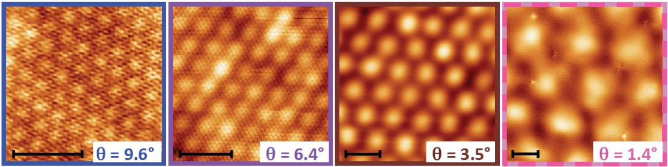
Figure 1: Scanning tunneling microscope images of tBLG moiré patterns. All scale bars are $5\,\text{nm}$. Source: Ref. (Brihuega2012, ).

For commensurate structures, ab initio numerical studies based on density functional theory have been performed (Latil2007, ; Morell2010, ; LaissardiereMayouMagaud2012, ). However, since the unit cell of the tBLG superlattice contains a large number of sites, especially at small $\theta$, these ab initio calculations incur a significant computational cost and are therefore rather unpractical. To avoid this difficulty, semi-analytical theories have been developed in order to describe the low-energy electronic properties of the tBLG. These theories focus mainly on the low-energy electronic states near the individual layer Dirac cones in a way that the model Hamiltonian describes Dirac electrons moving in each layer and hybridized by interlayer hopping. The first low-energy theory of this kind, which focused on the limit of small misalignment, was proposed by Lopes dos Santos et al. (Santos2007, ), and further developed in Ref. (Santos2012, ). A similar treatment based on a continuum approximation was done by Bistritzer and MacDonald (Bistritzer2011, ), generalizing the method to incommensurate structures. In Ref. (Gail2011, ), the authors made further simplifications to these low-energy Hamiltonians and derived an effective $2\times 2$ Hamiltonian, from which analytical expressions for the electronic spectrum can be obtained. A general description of incommensurate double layers, formed by any 2D materials and valid for arbitrary misalignment, was developed in Ref. (Koshino2015, ). This theory reduces to previous ones in the case of tBLG at small twist angle. More recently, in Ref. (Weckbecker2016, ), the authors proposed a model which is identical to that derived by Bistritzer and MacDonald, but with a rescaling in the coupling momentum scale, in better agreement with tight-binding ab initio calculations.

The chapter is organized as follows: in section II, we introduce basic concepts related to the theoretical description of graphene systems. Section III contains the derivation of a low-energy effective model for the tBLG, which is the starting point for the remaining work. In section IV, we compute the optical conductivity within the linear response theory and apply this result to the study of the spectrum of tBLG surface plasmon-polaritons. Finally, in section V, we present our main conclusions.

II Basics of monolayer and bilayer graphene

In this section, we start with a review of the tight-binding model for single layer graphene (SLG). This allows us to introduce general concepts and fix notation. We also analyze the description of SLG within a folded zone scheme, which will provide us a better understanding of the tBLG system. Finally, we briefly describe the properties of a particular stacking of bilayer graphene (BLG), the Bernal stacking. The description of an arbitrary arrangement of BLG, the tBLG, is left for the next section.

II.1 Single layer graphene

II.1.1 Lattice geometry

A SLG is a 2D layer made out of carbon atoms arranged into a honeycomb structure. We choose the coordinate system depicted in Fig. 2, such that the zig-zag direction is aligned with the $x$-axis and the armchair direction with the $y$-axis. Each unit cell contains two carbon atoms that belong to different sublattices, $A$ and $B$. The unit cells form a hexagonal Bravais lattice $\left\{\boldsymbol{R}\right\}$, with positions

$$\boldsymbol{R}=n_{1}\bm{a}_{1}+n_{2}\bm{a}_{2},\quad n_{1},n_{2}\in\mathbb{Z},$$ (2)

where the basis vectors $\bm{a}_{1}$ and $\bm{a}_{2}$ are given by

$$\bm{a}_{1}=a\left(1/2,\sqrt{3}/2\right),\quad\bm{a}_{2}=a\left(-1/2,\sqrt{3}/2\right),$$ (3)

and $a\simeq 2.46$\mathrm{\SIUnitSymbolAngstrom}$$ is the lattice parameter (GeimMacDonald2007, ), which is related to the carbon-carbon distance, $d$, by $a=\sqrt{3}d$. The area of the unit cell is

$$A_{u.c.}=\left|\bm{a}_{1}\times\bm{a}_{2}\right|=\frac{\sqrt{3}}{2}a^{2}.$$ (4)

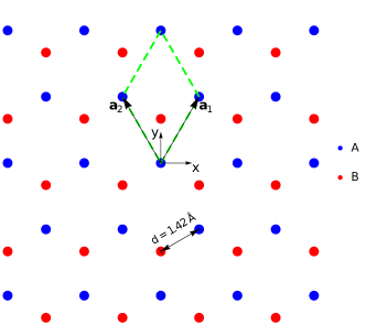
Figure 2: SLG geometry. The honeycomb structure can be seen as two interpenetrating hexagonal lattices, $A$ (blue) and $B$ (red). The dashed green line marks a unit cell of this system, which contains 2 atoms. The coordinate system is chosen to be centered at a carbon of sublattice $A$.

We will focus on systems with periodic boundary conditions, $N=\mathcal{N}_{1}\mathcal{N}_{2}$ unit cells (such that $n_{i}=0,1,...,\mathcal{N}_{i}-1$), in the limit of $\mathcal{N}_{i}\rightarrow\infty$.

II.1.2 Tight-binding model

We intend to describe the physical properties of a SLG. An isolated carbon atom has electronic configuration 1s²2s²2p². In graphene, from the four outer electrons, three of them are arranged in a $sp_{2}$ hybridization and form in-plane covalent $\sigma$ bonds between nearest neighbor carbon atoms. The remaining $p_{z}$ electron is delocalized. Most of the electronic properties of graphene are governed by the delocalized $p_{z}$ electrons. The relevant dynamics of these electrons can be accurately modeled within a simple single-orbital, nearest-neighbor tight-binding model (NetoGuineaPeresEtAl2009, ), which is the approach we shall also adopt here.

In the tight-binding approximation, we represent the electronic Hamiltonian in terms of an orthonormal atomic-like basis, the so-called Wannier states. In the second quantization formalism, a general tight-binding Hamiltonian can be written as

$$H=\sum_{\bm{R},\bm{\delta},\alpha,\beta}c_{\alpha}^{\dagger}\left(\bm{R}\right)h_{\bm{\delta}}^{\alpha\beta}c_{\beta}\left(\bm{R}+\bm{\delta}\right).$$ (5)

In this expression, $c_{\alpha}^{\dagger}(\bm{R})$ $\left(c_{\alpha}(\bm{R})\right)$ are creation (annihilation) operators for an electron in an atomic-like state of kind $\alpha$, which is centered at $\bm{R}+\bm{\tau}_{\alpha}$, where $\bm{R}$ is the position of the unit cell and $\bm{\tau}_{\alpha}$ is the relative position of the orbital center inside the unit cell. We will focus on spin independent models and therefore we have omitted the spin degree of freedom. Alternatively, this can be included into the index $\alpha$. We represent a state created by $c_{\alpha}^{\dagger}(\bm{R})$ as $\left|\bm{R},\alpha\right\rangle$ and we write the orbital in real space as $w_{\alpha}\left(\bm{r}-\bm{R}-\bm{\tau}_{\alpha}\right)$ (with $\bm{r}$ the position). $h_{\bm{\delta}}^{\alpha\beta}$ are hopping integrals, given by

$$h_{\bm{\delta}}^{\alpha\beta}=\left\langle\bm{R},\alpha\right|H\left|\bm{R}+\bm{\delta},\beta\right\rangle,$$ (6)

where $\bm{\delta}$ runs over neighboring unit cells. Translational invariance of the system has been assumed, which is manifest in the assumption that $h_{\bm{\delta}}^{\alpha\beta}$ is independent of $\bm{R}$. Due to the localization of the atomic-like orbitals, $h_{\bm{\delta}}^{\alpha\beta}$ decays very fast for large values of $\left|\bm{\delta}\right|$ and, therefore, we usually need to consider just a few hoppings to describe the electronic properties of the system.

In the single-orbital tight-binding model for graphene, we have two kinds of orbitals, the $p_{z}$ orbitals located at the $A$ and $B$ sites ($\alpha=A,B$), which, in the coordinate system of Fig. 2, are centered at positions $\bm{\tau}_{A}=(0,0)$ and $\bm{\tau}_{B}=(0,d)$. In the nearest-neighbor approximation, we only keep the on-site and nearest-neighbor hoppings,

$$h_{\bm{0}}^{AA} =h_{\bm{0}}^{BB}\equiv\epsilon_{p_{z}},$$ (7)

$$h_{\bm{\delta}_{NN}}^{AB} =h_{-\bm{\delta}_{NN}}^{BA}\equiv-t,$$ (8)

where $\bm{\delta}_{NN}$ are the vectors that, for any $A$ site, link its unit cell to the one of the corresponding nearest-neighbor $B$ sites, $\bm{\delta}_{NN}=\boldsymbol{0},\,-\bm{a}_{1},\,-\bm{a}_{2}$, and neglect all other hoppings. According to ab initio calculations, $t=2.97$\mathrm{eV}$$ (Reich2002, ). Without loss of generality, we can redefine the zero of energy to coincide with the on-site energy and therefore set $\epsilon_{p_{z}}=0$. The tight-binding Hamiltonian for SLG is thus written as

$$H=-t\sum_{\bm{R}}c_{A}^{\dagger}\left(\bm{R}\right)\left(c_{A}\left(\bm{R}\right)+c_{B}\left(\bm{R}-\bm{a}_{1}\right)+c_{B}\left(\bm{R}-\bm{a}_{2}\right)\right)+\text{h.c.},$$ (9)

where h.c. stands for hermitian conjugate.

In order to diagonalize the Hamiltonian, we make use of Bloch’s theorem. Bloch’s theorem states that, in a periodic system, the electron wavefunction has the form of a Bloch wave,

$$\psi_{\bm{k},n}(\bm{r})=e^{i\bm{k}\cdot\bm{r}}u_{\bm{k},n}(\bm{r}),$$ (10)

where $\bm{k}$ is the crystal or Bloch momentum, $n$ is a band index and $u_{\bm{k},n}(\bm{r})$ a periodic function with the same periodicity of the crystal, i.e., $u_{\bm{k},n}(\bm{r})=u_{\bm{k},n}(\bm{r}+\bm{R})$ for all crystal lattice vectors $\bm{R}$. An equivalent statement of Bloch’s theorem is that electronic states in a periodic system satisfy

$$\psi_{\bm{k},n}(\bm{r}+\bm{R})=e^{i\bm{k}\cdot\bm{R}}\psi_{\bm{k},n}(\bm{r}),$$ (11)

being eigenstates of the lattice translation operator with corresponding eigenvalue $e^{i\bm{k}\cdot\bm{R}}$. Graphene wavefunctions that satisfy Bloch’s theorem can be written in the localized basis as

$$\psi_{\bm{k},\alpha}(\bm{r})=\frac{1}{\sqrt{N}}\sum_{\bm{R}}e^{i\bm{k}\cdot\left(\bm{R}+\bm{\tau}_{\alpha}\right)}w_{\alpha}\left(\bm{r}-\bm{R}-\bm{\tau}_{\alpha}\right),$$ (12)

or, in bra-ket notation,

$$\left|\psi_{\bm{k},\alpha}\right\rangle=\frac{1}{\sqrt{N}}\sum_{\bm{R}}e^{i\bm{k}\cdot\left(\bm{R}+\bm{\tau}_{\alpha}\right)}\left|\bm{R},\alpha\right\rangle.$$ (13)

In general, eigenstates will be a superposition of states involving all atomic-like orbitals. Therefore, we look for eigenstates of the SLG Hamiltonian, Eq. (9), in the general form

$$\left|\psi_{\bm{k}}\right\rangle=\sum_{\alpha}u_{\alpha}(\bm{k})\left|\psi_{\bm{k},\alpha}\right\rangle,$$ (14)

where $u_{\alpha}(\bm{k})$ are complex amplitudes. Note that there is some arbitrariness in these expressions, since we can drop the phase $e^{i\bm{k}\cdot\bm{\tau}_{\alpha}}$ in Eq. (13) and include it in the complex amplitudes $u_{\alpha}(\bm{k})$ in Eq. (14) (BenaMontambaux2009, ). Obviously, no physical quantity can depend on this choice, but the representation of operators can. The convention used in Eq. (13) simplifies the representation of the current operator within the tight-binding model (Indranil2003, ) and we will therefore stick to it.

From the time-independent single-particle Schrödinger equation,

$$H\left|\psi\right\rangle=E\left|\psi\right\rangle,$$ (15)

where $E$ is the energy, choosing $\left|\psi\right\rangle$ of the form of Eq. (13) and applying the bras $\left\langle\bm{R},A\right|$ and $\left\langle\bm{R},B\right|$ (for any $\bm{R}$), we end up with a closed system of equations that we conveniently write in a matrix form,

$$H(\bm{k})\cdot\begin{bmatrix}u_{A}(\bm{k})\\ u_{B}(\bm{k})\end{bmatrix}=E\begin{bmatrix}u_{A}(\bm{k})\\ u_{B}(\bm{k})\end{bmatrix},$$ (16)

where $H(\bm{k})$ is the Hamiltonian in the $\left|\psi_{\bm{k},A}\right\rangle,\left|\psi_{\bm{k},B}\right\rangle$ basis,

$$H(\bm{k})=\begin{bmatrix}0&-tf(\bm{k})\\ -tf^{*}(\bm{k})&0\end{bmatrix},$$ (17)

with

$$f(\bm{k})=\sum_{i=1}^{3}e^{i\bm{k}\cdot\bm{d}_{i}},$$ (18)

in which $\bm{d}_{1}=\left(\bm{a}_{1}+\bm{a}_{2}\right)/3$, $\bm{d}_{2}=\left(-2\bm{a}_{1}+\bm{a}_{2}\right)/3$, $\bm{d}_{3}=\left(\bm{a}_{1}-2\bm{a}_{2}\right)/3$ are the positions of the three nearest neighboring $B$ sites to an $A$ site and ^∗ stands for complex conjugate. The eigenvalues of $H(\bm{k})$ are given by

$$E_{\pm}(\bm{k})=\pm t\sqrt{4\cos\left(\frac{\sqrt{3}}{2}dk_{x}\right)\cos\left(\frac{3}{2}dk_{y}\right)+2\cos\left(\sqrt{3}dk_{x}\right)+3}.$$ (19)

This spectrum is represented in Fig. 3(b).

II.1.3 Low-energy Dirac Hamiltonian

If we are only interested in the low-energy properties of graphene, which are the most relevant experimentally, a simplified Hamiltonian can be obtained. As we can see in Fig. 3(b), the spectrum of SLG is gapless with the two bands touching at the two inequivalent corners of the Brillouin zone (BZ): the K and K${}^{\prime}=-$K points, with

$$\text{K}=\frac{4\pi}{3\sqrt{3}d}\left(1,0\right).$$ (20)

In neutral graphene, we have one $p_{z}$ electron, per carbon atom, contributing to the electronic structure. Also, we know that we have as many bands as atoms in the unit cell and that every state gets filled with two electrons, due to spin degeneracy. Therefore, the neutral configuration corresponds to the situation where half of the bands are filled, by increasing order of energy. This implies that, in neutral graphene, the band $E_{-}(\bm{k})$ is completely full and the band $E_{+}(\bm{k})$ is empty, with the Fermi level lying at $E=0$ and intersecting the bands at K and K^′. The physics of graphene is thus dominated by electronic states close to these points. Writing the electronic Bloch-momentum as $\bm{k}=\pm\text{K}+\bm{q}$ and Taylor expanding to lowest order in $\bm{q}$, we obtain the low-energy Hamiltonian

$$H^{\pm\text{K}}(\bm{q})=\hbar v_{F}\begin{bmatrix}0&\pm q_{x}-iq_{y}\\ \pm q_{x}+iq_{y}&0\end{bmatrix}=\hbar v_{F}\bm{q}\cdot\left(\pm\sigma_{x},\sigma_{y}\right),$$ (21)

where the Fermi velocity, $v_{F}$, is identified as $v_{F}=\frac{3td}{2\hbar}$, $\hbar$ is the reduced Planck constant, $\sigma_{x}$ and $\sigma_{y}$ are Pauli matrices and the $\pm$ sign indicates the point around which the expansion is made. This low-energy Hamiltonian is recognized as a (massless) Dirac Hamiltonian and for this reason the K and K^′ points are called Dirac points.

II.1.4 Reciprocal space and folded band description

Given the real space direct lattice, Eq. (2), we can define a set of points $\left\{\bm{G}\right\}$ such that $e^{i\bm{G}\cdot\bm{R}}=1$. These points also form a lattice, which is referred to as reciprocal lattice. The points of the reciprocal lattice $\left\{\bm{G}\right\}$ can be written in terms of a basis as

$$\bm{G}=m_{1}\bm{b}_{1}+m_{2}\bm{b}_{2},\quad m_{1},m_{2}\in\mathbb{Z},$$ (22)

where the reciprocal lattice basis vectors $\bm{b}_{1}$ and $\bm{b}_{2}$ obey, by definition, the relation

$$\bm{a}_{i}\cdot\bm{b}_{j}=2\pi\delta_{i,j}.$$ (23)

For graphene, this leads to

$$\bm{b}_{1}=\frac{4\pi}{3d}\left(\sqrt{3}/2,1/2\right),\quad\bm{b}_{2}=\frac{4\pi}{3d}\left(-\sqrt{3}/2,1/2\right).$$ (24)

The reciprocal lattice for SLG is shown in Fig. 3(a).

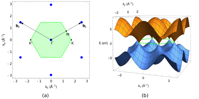
Figure 3: SLG reciprocal space (a) and electronic spectrum (b). In (a), the blue circles represent points in the reciprocal lattice; just like the direct lattice, the reciprocal one is also hexagonal, though rotated and with a different lattice parameter. The green primitive unit cell marks the first BZ; some relevant points are represented in it: $\text{$\Gamma$}=(0,0)$, $\text{M}=\left(1,1/\sqrt{3}\right)\frac{\pi}{a}$, $\text{K}=\left(\frac{4\pi}{3a},0\right)$, $\text{K}^{\prime}=-\text{K}$. The green dashed line marks the first BZ boundaries.

By definition, Bloch states are unchanged under shifts of the crystal-momentum by a reciprocal lattice vector, $\bm{k}\rightarrow\bm{k}+\bm{G}$. This means that the electronic properties of a periodic system are completely characterized if we focus on crystal-momenta that are restricted to a unit cell in reciprocal space, the first BZ.

We now notice that, for the geometry described in Fig. 2, we are free to pick a larger unit cell, with a corresponding smaller BZ, provided that this cell captures the periodicity of the system. As an example, we consider unit cells with the shape of a rhombus containing $2\times 3^{p}$ ($p\in\mathbb{N}$) carbon atoms. The basis vectors for the corresponding lattice are given by

$$\bm{a}_{1}^{(p)} =\sqrt{3}^{p+1}d\begin{cases}\left(1/2,\sqrt{3}/2\right)&\text{if }p\text{ is even}\\ \left(\sqrt{3}/2,1/2\right)&\text{if }p\text{ is odd}\end{cases},$$ (25)

$$\bm{a}_{2}^{(p)} =\sqrt{3}^{p+1}d\begin{cases}\left(-1/2,\sqrt{3}/2\right)&\text{if }p\text{ is even}\\ \left(-\sqrt{3}/2,1/2\right)&\text{if }p\text{ is odd}\end{cases}.$$ (26)

For $p=0$ we recover the minimal unit cell. The enlarged unit cells for $p=1$ and $p=2$ are shown in Fig. 4. The corresponding reciprocal lattice vectors are

$$\bm{b}_{1}^{(p)} =\frac{4\pi}{\sqrt{3}^{p}3d}\begin{cases}\left(\sqrt{3}/2,1/2\right)&\text{if }p\text{ is even}\\ \left(1/2,\sqrt{3}/2\right)&\text{if }p\text{ is odd}\end{cases},$$ (27)

$$\bm{b}_{2}^{(p)} =\frac{4\pi}{\sqrt{3}^{p}3d}\begin{cases}\left(-\sqrt{3}/2,1/2\right)&\text{if }p\text{ is even}\\ \left(-1/2,\sqrt{3}/2\right)&\text{if }p\text{ is odd}\end{cases}.$$ (28)

It is apparent that, as the unit cell size and $\left|\bm{a}_{i}^{(p)}\right|$ increase, $\left|\bm{b}_{i}^{(p)}\right|$ and the corresponding BZ become smaller. At the same time, the number of sublattice sites in the unit cell increases from $2$ to $2\times 3^{p}$, which leads to $2\times 3^{p}$ bands. Since the system being described is always the same, these additional bands are obtained by folding the original bands into the smaller BZ.

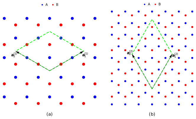
Figure 4: Basis vectors and unit cells for a folded band description of SLG with (a) $p=1$ (6-atom unit cell), (b) $p=2$ (18-atom unit cell).

We now wish to write the Hamiltonian in reciprocal space for the case of an enlarged unit cell. We could always rewrite the Hamiltonian for the larger unit cell in direct space and then follow the same procedure as in section II.1.2. However, we will follow an alternative approach. We expect that it should be possible to write the folded Hamiltonian directly in reciprocal space in terms of the Bloch waves defined for the unfolded one. We first discuss the $p=1$ case. By inspecting Fig. 5(a), and according to the previous discussion, we see that, when using the enlarged unit cell, we are reducing the size of the BZ by $1/3$. Although the description is different, the overall system is the same. Hence, the information from regions $2$ and $3$ of the original BZ must be encoded into the reduced BZ (region $1$). Let us now imagine that we already have the Hamiltonian for the folded case. Since we have six atoms per unit cell, we must have six bands. If we then represent the spectrum using an extended zone scheme —the first two bands in the first BZ, the second ones in the second BZ and the third ones in the third BZ— we obtain a spectrum that coincides exactly with the unfolded one. This provides a way of putting the information from regions $2$ and $3$ into $1$. We observe that, for each $\bm{k}$ in region $1$, we can get to regions $2$ and $3$ (or equivalent regions) by translations of $\bm{b}_{1}^{(1)}$ and $\bm{b}_{2}^{(1)}$.

Recalling the unfolded original Hamiltonian,

$$H_{\bm{k}}^{(0)}=\begin{bmatrix}0&-tf(\bm{k})\\ -tf^{*}(\bm{k})&0\end{bmatrix},$$ (29)

we may now write the folded Hamiltonian in the enlarged basis, $\left|\bm{k}\right\rangle$, $\left|\bm{k}+\bm{b}_{1}^{(1)}\right\rangle$, $\left|\bm{k}+\bm{b}_{2}^{(1)}\right\rangle$, as

$$H_{\bm{k}}^{(1)}=\begin{bmatrix}H_{\bm{k}}^{(0)}&0&0\\ 0&H_{\bm{k}+\bm{b}_{1}^{(1)}}^{(0)}&0\\ 0&0&H_{\bm{k}+\bm{b}_{2}^{(1)}}^{(0)}\end{bmatrix}.$$ (30)

For a given $p>0$, it is straightforward to generalize and write

$$H_{\bm{k}}^{(p)}=\begin{bmatrix}H_{\bm{k}}^{(p-1)}&0&0\\ 0&H_{\bm{k}+\bm{b}_{1}^{(p)}}^{(p-1)}&0\\ 0&0&H_{\bm{k}+\bm{b}_{2}^{(p)}}^{(p-1)}\end{bmatrix}.$$ (31)

Note that inside $H^{(p)}$, we have information of all Hamiltonians back to the original one, $H^{(0)}$.

In Fig. 5(b), we plot the eigenvalues for both the original and $1/3$ folded Hamiltonians. This construction will be useful to understand the tBLG, as we will see in section III.3.2.

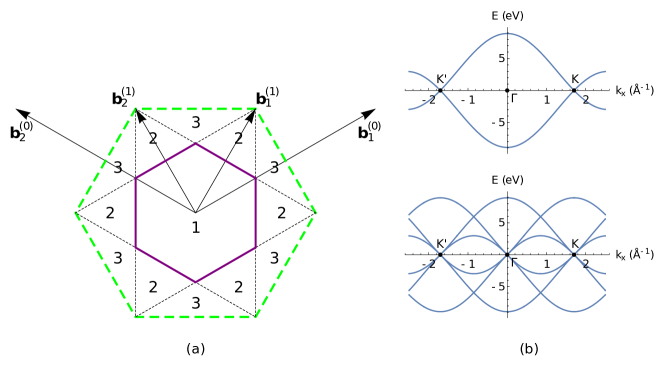
Figure 5: (a) Reciprocal space folding scheme. The green dashed line marks the original BZ, while the purple line marks the BZ for a $p=1$ folding. Regions labeled by $1$, $2$ and $3$ correspond to the first, second and third BZs for the folded case. (b) Electronic spectrum of SLG for $p=0$ (top) and $p=1$ (bottom). Plots with $k_{y}=0$.

II.1.5 Density of states and carrier density profile

We finish the discussion of the SLG addressing two quantities —the density of states (DOS) and the carrier density profile— that help to characterize the electronic structure of the system when doped with electrons or holes. By definition, the DOS describes the number of states, per interval of energy, at each energy level, available to be occupied. As for the carrier density profile, it defines the relation between the density of carriers $n$ (positive for electrons, negative for holes) that is needed to reach a given Fermi level $\mu$; this is a useful quantity since the carrier density is the parameter well defined in experimental results. Given the electronic spectrum, both the DOS and the carrier density profile can be calculated in a straightforward manner.

Results for the DOS and carrier density profile in SLG are presented in Fig. 6. We first address the carrier density. Experimentally, record values up to $\left|n\right|\sim 4\times 10^{14}${\mathrm{cm}}^{-2}$$ have been reported (Efetov2010, ). Nevertheless, under ambient conditions, typical values for doping are one order of magnitude below (Das2008, ; Mak2009, ). We will stick within this range, which corresponds to the zoomed region in Fig. 6(b). As can be seen from this inset, the corresponding Fermi level is far away from what is needed to reach the peaks in the DOS —the so-called van Hove singularities—, making them inaccessible. This is a big downside since electronic instabilities that can lead to new phases of matter are expected when we cross a van Hove singularity (Fleck1997, ; Gonzalez2008, ; Nandkishore2012, ). One of the reasons that motivates the study of tBLG systems is precisely the fact that we can bring van Hove singularities to arbitrarily low energies by varying the twist angle (Li2010, ).

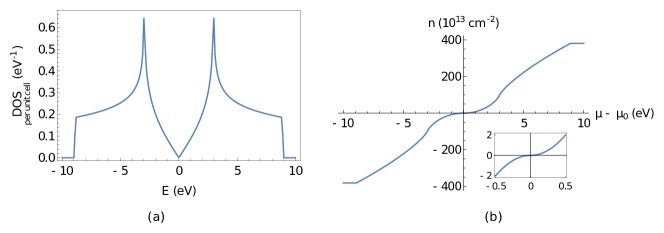
Figure 6: DOS (a) and carrier density profile (b) for SLG. (a) shows the DOS per unit cell. In (b), $\mu_{0}$ is the Fermi level for neutral graphene.

II.2 Introduction to bilayers: Bernal-stacked bilayer graphene

II.2.1 Structure

A BLG is a stacking of two SLGs, where the typical experimental interlayer distance is $d_{\perp}=3.35$\mathrm{\SIUnitSymbolAngstrom}$$ (RozhkovSboychakovRakhmanovEtAl2015, ). Among the possible stacking arrangements, two are worth pointing out: 1) AA stacking, where each carbon atom from the top layer is placed exactly above its correspondent in the bottom layer; 2) AB stacking, or Bernal stacking, which is obtained by sliding one of the layers with respect to the other along the armchair direction, such that the atoms of sublattice $A$ from one layer are aligned with the atoms of sublattice $B$ from the other layer, implying the remaining to be located in the center of the hexagons (Fig. 7). Both AA and AB stacking share the same Bravais lattice structure with SLG, having the same unit cell. Experimentally, the AA stacking is considered metastable, while both the Bernal stacking and the tBLG are found to be stable (RozhkovSboychakovRakhmanovEtAl2015, ). In this section, we analyze the electronic properties of Bernal-stacked BLG.

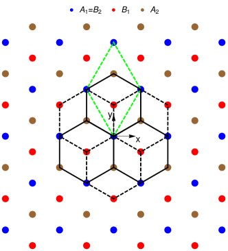
Figure 7: Bernal-stacked BLG geometry (top view). We label the bottom layer (dashed black lines) as 1 and the top layer (solid black lines) as 2. The unit cell used for the SLG (green dashed line) is maintained, keeping both direct and reciprocal space descriptions identical as before, except that each unit cell now contains four atoms.

II.2.2 Tight-binding model

To model this system, we retain the approximations used before for each individual layer; in addition, we take into account interlayer hopping, in a transversal tight-binding approximation between nearest-neighbors. We start by writing the Hamiltonian for the bilayer as a sum of three terms,

$$H=H_{1}+H_{2}+H_{\perp},$$ (32)

where $H_{\ell}$ is the Hamiltonian for each individual layer $\ell=1,2$, while $H_{\perp}$ takes into account interlayer coupling. In the second quantized formalism, using the same approximations as for the SLG case (Eq. (9)), we obtain

$$H_{1} =-t\sum_{\bm{R}}c_{1,A}^{\dagger}\left(\bm{R}\right)\left[c_{1,B}\left(\bm{R}\right)+c_{1,B}\left(\bm{R}-\bm{a}_{1}\right)+c_{1,B}\left(\bm{R}-\bm{a}_{2}\right)\right]+\text{h.c.},$$ (33)

$$H_{2} =-t\sum_{\bm{R}}c_{2,A}^{\dagger}\left(\bm{R}\right)\left[c_{2,B}\left(\bm{R}\right)+c_{2,B}\left(\bm{R}-\bm{a}_{1}\right)+c_{2,B}\left(\bm{R}-\bm{a}_{2}\right)\right]+\text{h.c.},$$ (34)

where $c_{\ell,\alpha}^{\dagger}\left(\bm{R}\right)/c_{\ell,\alpha}\left(\bm{R}\right)$ is the creation/annihilation fermionic operator for an electron in a atomic-like state $\left|\ell,\bm{R},\alpha\right\rangle$ located at cell $\bm{R}$, sublattice $\alpha$ and layer $\ell$. For $H_{\perp}$, we consider a homogeneous interlayer hopping, $t_{\perp}$, between nearest neighbors only,

$$\left\langle 1,\bm{R},A\right|H_{\perp}\left|2,\bm{R},B\right\rangle=t_{\perp},$$ (35)

and set $t_{\perp}=0.33$\mathrm{eV}$$, which is compatible with the range of estimated values (RozhkovSboychakovRakhmanovEtAl2015, ). In the second quantized formalism, we can thus write

$$H_{\perp}=t_{\perp}\sum_{\bm{R}}c_{1,A}^{\dagger}\left(\bm{R}\right)c_{2,B}\left(\bm{R}\right)+\text{h.c.}.$$ (36)

We now move to the reciprocal space and write the Hamiltonian in terms of fermionic operators of electronic states of the Bloch form,

$$\left|\psi_{\ell,\bm{k},\alpha}\right\rangle=\frac{1}{\sqrt{N}}\sum_{\bm{R}}e^{i\bm{k}\cdot\left(\bm{R}+\bm{\tau}_{\ell,\alpha}\right)}\left|\ell,\bm{R},\alpha\right\rangle,$$ (37)

where $\bm{\tau}_{\ell,\alpha}$ are the in-plane positions of the four carbon atoms in the unit cell, which read as $\bm{\tau}_{1,A}=\bm{\tau}_{2,B}=\left(0,0\right)$ and $\bm{\tau}_{1,B}=-\bm{\tau}_{2,A}=\left(0,d\right)$. The corresponding creation operators can be written as

$$c_{\ell,\alpha}^{\dagger}(\bm{k})=\frac{1}{\sqrt{N}}\sum_{\bm{R}}e^{i\bm{k}\cdot\left(\bm{R}+\bm{\tau}_{\ell,\alpha}\right)}c_{\ell,\alpha}^{\dagger}(\bm{R}),$$ (38)

which can be understood as a discrete Fourier Transform of the operators $c_{\ell,\alpha}^{\dagger}(\bm{R})$. Using the property

$$\sum_{\bm{R}}e^{i\bm{R}\cdot\left(\bm{k}-\bm{k}^{\prime}\right)}=N\sum_{\bm{G}}\delta_{\bm{k}-\bm{k}^{\prime},\bm{G}},$$ (39)

which for $\bm{k},\bm{k}^{\prime}\in\text{BZ}$ yields $\sum_{\bm{R}}e^{i\bm{R}\cdot\left(\bm{k}-\bm{k}^{\prime}\right)}=N\delta_{\bm{k},\bm{k}^{\prime}}$, we can invert Eq. (38), obtaining

$$c_{\ell,\alpha}^{\dagger}(\bm{R})=\frac{1}{\sqrt{N}}\sum_{\bm{k}}e^{-i\bm{k}\cdot\left(\bm{R}+\bm{\tau}_{\ell,\alpha}\right)}c_{\ell,\alpha}^{\dagger}(\bm{k}),$$ (40)

where the sum (which becomes an integral in the limit of an infinite crystal) is restricted to the first BZ. Therefore, we can write the Hamiltonian in a second quantized form as

$$H=\sum_{\bm{k}}\Psi^{\dagger}(\bm{k})\cdot H(\bm{k})\cdot\Psi(\bm{k}),$$ (41)

where we have introduced $\Psi^{\dagger}(\bm{k})=\left[\begin{array}[]{cccc}c_{1,A}^{\dagger}(\bm{k})&c_{1,B}^{\dagger}(\bm{k})&c_{2,A}^{\dagger}(\bm{k})&c_{2,B}^{\dagger}(\bm{k})\end{array}\right]$ and

$$H(\bm{k})=\left[\begin{array}[]{cccc}0&-tf(\bm{k})&0&t_{\perp}\\ -tf^{*}(\bm{k})&0&0&0\\ 0&0&0&-tf(\bm{k})\\ t_{\perp}&0&-tf^{*}(\bm{k})&0\end{array}\right].$$ (42)

Diagonalizing $H(\bm{k})$, we obtain the electronic spectrum for Bernal-stacked BLG as four bands,

$$E_{\pm,\pm}(\bm{k})=\pm t\sqrt{\left(\frac{t_{\perp}}{2t}\right)^{2}+4\cos\left(\frac{\sqrt{3}}{2}dk_{x}\right)\cos\left(\frac{3}{2}dk_{y}\right)+2\cos\left(\sqrt{3}dk_{x}\right)+3}\pm\frac{t_{\perp}}{2}.$$ (43)

The pair of bands $E_{+,-}(\bm{k})$ and $E_{-,+}(\bm{k})$ are gapless and touch at the K and K^′ points of the BZ. We show the obtained band structure along a representative path in first BZ in Fig. 8.

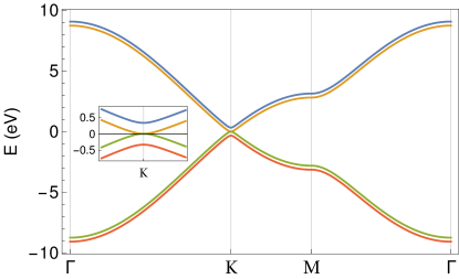
Figure 8: Electronic spectrum for Bernal-stacked BLG, along the $\bm{k}$-space trajectory $\text{$\Gamma$}\rightarrow\text{K}\rightarrow\text{M}\rightarrow\text{$\Gamma$}$.

III Twisted bilayer graphene

In this section, we aim at deriving a model for the tBLG system. We follow the work done by Bistritzer and MacDonald (Bistritzer2011, ) and construct a continuum low-energy effective Hamiltonian, which is valid for twist angles $\theta\lesssim 10^{\circ}$ and independent of the structure being commensurate or incommensurate. The electronic properties of this system are then addressed.

III.1 Geometry and moiré pattern

We begin by establishing a general geometry for a tBLG. A completely arbitrary arrangement can be achieved in the following manner: we start with a perfectly aligned BLG (for concreteness we take this to be Bernal-stacked) and, with one of the layers fixed, which we will refer to as layer 1, we translate the second, layer 2, by a vector $\bm{\tau}_{0}$ and then rotate it by an angle $\theta$ (anti-clockwise and about the origin). This way, each layer $\ell=1,2$ is described by the following lattice points:

$$\bm{R}_{\ell}=n_{1}\bm{a}_{\ell,1}+n_{2}\bm{a}_{\ell,2},\quad n_{1},n_{2}\in\mathbb{Z},$$ (44)

where $\bm{a}_{\ell,1}$ and $\bm{a}_{\ell,2}$ are the basis vectors of each layer, which are related by $\bm{a}_{2,i}=\mathcal{R}_{\theta}\cdot\bm{a}_{1,i}$, where $\mathcal{R}_{\theta}$ is the rotation matrix that describes an anti-clockwise rotation by $\theta$ about the origin of a 2D coordinate system,

$$\mathcal{R}_{\theta}=\begin{bmatrix}\cos(\theta)&-\sin(\theta)\\ \sin(\theta)&\cos(\theta)\end{bmatrix}.$$ (45)

The positions of the $A$ and $B$ sites for each layer are given by

$$\bm{\tau}_{1,A}=\left(0,0\right), \bm{\tau}_{2,A}=\mathcal{R}_{\theta}\cdot\left[\left(0,-d\right)+\bm{\tau}_{0}\right],$$ (46)

$$\bm{\tau}_{1,B}=\left(0,d\right), \bm{\tau}_{2,B}=\mathcal{R}_{\theta}\cdot\left[\left(0,0\right)+\bm{\tau}_{0}\right].$$ (47)

Associated to the lattices $\left\{\bm{R}_{\ell}\right\}$, we have the corresponding reciprocal lattices $\left\{\bm{G}_{\ell}\right\}$ which are spanned by the vectors $\bm{b}_{\ell,1}$, and $\bm{b}_{\ell,2}$. The reciprocal lattice basis vectors are also related via rotation as $\bm{b}_{2,i}=\mathcal{R}_{\theta}\cdot\bm{b}_{1,i}$.

The distinct periodicity of the two layers gives origin to an interference effect that leads to the formation of a moiré pattern. The moiré pattern is nothing more than a beat effect (SanJose2014, ) and can be understood as follows. Let us consider two functions $h_{1}(\bm{r})$ and $h_{2}(\bm{r})$ with the same periodicity as the layers $1$ and $2$, respectively. We choose these functions as

$$h_{\ell}(\bm{r})=\sum_{k=1}^{3}\cos\left(\bm{G}_{\ell,k}\cdot\bm{r}\right),$$ (48)

where we have written $\bm{G}_{\ell,1}=\bm{b}_{\ell,1}$, $\bm{G}_{\ell,2}=\bm{b}_{\ell,2}$, $\bm{G}_{\ell,3}=\bm{b}_{\ell,1}-\bm{b}_{\ell,2}$. We can study the interference effects between the two layers by studying the function $h_{m}(\bm{r})=h_{1}(\bm{r})+h_{2}(\bm{r})$. Standard manipulation allows us to write

$$h_{m}(\bm{r})=\sum_{k=1}^{3}2\cos\left(\frac{\bm{G}_{1,k}+\bm{G}_{2,k}}{2}\cdot\bm{r}\right)\cos\left(\frac{\bm{G}_{1,k}-\bm{G}_{2,k}}{2}\cdot\bm{r}\right).$$ (49)

Therefore, we see that the function will have fast oscillations controlled by $\left(\bm{G}_{1,k}+\bm{G}_{2,k}\right)/2$, which are modulated by a slowly oscillating envelop function that oscillates with $\left(\bm{G}_{1,k}-\bm{G}_{2,k}\right)/2$. It is this envelop function that is responsible for the moiré pattern. Given that only the amplitude (and not the sign) of the envelop affects the visibility of the moiré pattern, this appears to oscillate with $\bm{G}_{1,k}-\bm{G}_{2,k}$. For this same reason, the moiré pattern is not affected by the translations of one layer with respect to the other. Therefore, the function $h_{m}(\bm{r})$ will display a quasi-periodic pattern, with an associated reciprocal lattice $\left\{\bm{G}^{m}\right\}$ that is spanned by the moiré basis vectors

$$\bm{b}_{1}^{m}=\bm{b}_{1,1}-\bm{b}_{2,1},\quad\bm{b}_{2}^{m}=\bm{b}_{1,2}-\bm{b}_{2,2}.$$ (50)

In the coordinate system where layer 2 is rotated by $\theta/2$ and layer 1 is rotated by $-\theta/2$, these are given by

$$\bm{b}_{1}^{m}=\sqrt{3}\left|\Delta\text{K}\right|\left(\frac{1}{2},-\frac{\sqrt{3}}{2}\right),\quad\bm{b}_{2}^{m}=\sqrt{3}\left|\Delta\text{K}\right|\left(\frac{1}{2},\frac{\sqrt{3}}{2}\right),$$ (51)

where $\left|\Delta\text{K}\right|=2\text{$\left|\text{K}\right|$}\sin\left(\theta/2\right)$ is the separation between the Dirac points of the two layers, with $\text{$\left|\text{K}\right|$}=4\pi/\left(3\sqrt{3}d\right)$.

Associated to the reciprocal lattice $\left\{\bm{G}^{m}\right\}$, we can define a moiré real lattice $\left\{\bm{R}^{m}\right\}$, spanned by basis vectors $\bm{a}_{1}^{m}$ and $\bm{a}_{2}^{m}$, such that $\bm{a}_{i}^{m}\cdot\bm{b}_{j}^{m}=2\pi\delta_{i,j}$, which are explicitly given by

$$\bm{a}_{1}^{m}=\frac{4\pi}{3\left|\Delta\text{K}\right|}\left(\frac{\sqrt{3}}{2},-\frac{1}{2}\right),\quad\bm{a}_{2}^{m}=\frac{4\pi}{3\left|\Delta\text{K}\right|}\left(\frac{\sqrt{3}}{2},\frac{1}{2}\right).$$ (52)

The unit cell of the moiré lattice has area

$$A_{m.u.c.}=\left|\bm{a}_{1}^{m}\times\bm{a}_{2}^{m}\right|=\frac{\sqrt{3}}{2}\left(\frac{4\pi}{3\left|\Delta\text{K}\right|}\right)^{2}=\frac{3\sqrt{3}d^{2}}{8\sin^{2}(\theta/2)}.$$ (53)

In Fig. 9, we show an example of the emergence of a moiré pattern in the function $h_{m}(\bm{r})$ and compare it to the moiré pattern that appears when the two lattices that form a tBLG structure are superimposed.

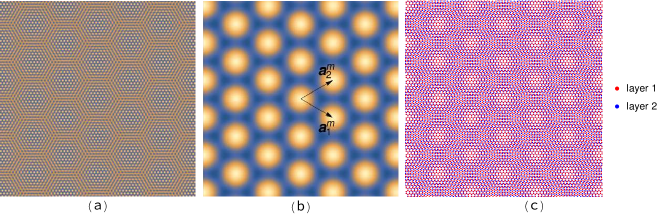
Figure 9: Formation of moiré pattern due to the interference of two periodic structures. (a) Density plot of the function $h_{m}(\bm{r})$. (b) Density plot of the envelop function $\tilde{h}_{m}(\bm{r})=\sum_{k=1}^{3}2\cos\left[\left(\bm{G}_{1,k}-\bm{G}_{2,k}\right)\cdot\bm{r}\right]$. The basis vectors of the moiré lattice are also shown. (c) Representation of the structure of tBLG. The emergence of the moiré pattern is clear. In all plots it was considered a twist angle $\theta=5^{\circ}$ (layer 2 rotated by $\theta/2$, layer 1 rotated by $-\theta/2$) and $\bm{\tau}_{0}=\left(0,d\right)$, such that in the unrotated limit, AB stacked BLG is recovered. The consideration of different values of $\bm{\tau}_{0}$ just leads to a shift in real space of the moiré pattern.

III.2 Model Hamiltonian

We will now see how a tBLG structure can be modeled. The approach described here closely follows the work of Ref. (Bistritzer2011, ) for tBLG in the small angle limit, which was generalized for other materials and arbitrary angles in Ref. (Koshino2015, ). The starting point of the method is a tight-binding representation of the Hamiltonian, which is partitioned as

$$H=H_{1}+H_{2}+H_{\perp},$$ (54)

where $H_{\ell}$ is the Hamiltonian of the isolated layer $\ell=1,2$ and $H_{\perp}=V_{12}+V_{21}$ is the interlayer Hamiltonian, which describes hybridization between the two layers. $V_{12}$ describes electron hopping from layer $2$ to layer $1$ and $V_{21}=V_{12}^{\dagger}$ describes the inverse process. The general approach is based on a two-center approximation for the interlayer Hamiltonian and in an expansion of the full Hamiltonian in terms of Bloch waves of the individual layers.

III.2.1 Hamiltonian for rotated graphene monolayers

We want to express the full Hamiltonian in terms of Bloch waves for the individual layers of the form of Eqs. (13) and (37),

$$\left|\psi_{\ell,\bm{k},\alpha}\right\rangle=\frac{1}{\sqrt{N_{\ell}}}\sum_{\bm{R}_{\ell}}e^{i\bm{k}\cdot\left(\bm{R}_{\ell}+\bm{\tau}_{\ell,\alpha}\right)}\left|\ell,\bm{R}_{\ell},\alpha\right\rangle,$$ (55)

where $\ell=1,2$ labels the layer, $\alpha=A,B$ is the sublattice, $N_{\ell}$ is the number of unit cells of each layer, $\bm{R}_{\ell}$ are the lattice sites, $\bm{\tau}_{\ell,\alpha}$ are the positions of the orbital centers in the unit cell and $\left|\ell,\bm{R}_{\ell},\alpha\right\rangle$ are localized atomic-like Wannier states. In this basis, and in the single-orbital nearest-neighbor approximation, the Hamiltonian for each layer reads as

$$H_{\ell}(\bm{k})=\begin{bmatrix}0&-tf_{\ell}(\bm{k})\\ -tf_{\ell}^{*}(\bm{k})&0\end{bmatrix},$$ (56)

where $f_{\ell}(\bm{k})=\sum_{i=1}^{3}e^{i\bm{k}\cdot\bm{d}_{\ell,i}}$, with $\bm{d}_{\ell,1}=\left(\bm{a}_{\ell,1}+\bm{a}_{\ell,2}\right)/3$, $\bm{d}_{\ell,2}=\left(-2\bm{a}_{\ell,1}+\bm{a}_{\ell,2}\right)/3$, $\bm{d}_{\ell,3}=\left(\bm{a}_{\ell,1}-2\bm{a}_{\ell,2}\right)/3$.

If we are interested in low-energy states, we can describe each layer with a Dirac Hamiltonian by writing $\bm{k}=\pm\text{K}_{\ell}+\bm{q}$, where $\pm\text{K}_{\ell}$ points are the Dirac points of each layer with $\text{K}_{1}=\left(\frac{4\pi}{3a},0\right)$ and $\text{K}_{2}=\mathcal{R}_{\theta}\cdot\text{K}_{1}$, and expanding to lowest order in $\bm{q}$. The obtained Hamiltonians can be written in a unified way as

$$H_{\ell}^{\pm\text{K}}(\bm{q})=\pm\hbar v_{F}\left|\bm{q}\right|\left[\begin{array}[]{cc}0&e^{\mp i\left(\theta_{\bm{q}}-\theta_{\ell}\right)}\\ e^{\pm i\left(\theta_{\bm{q}}-\theta_{\ell}\right)}&0\end{array}\right],$$ (57)

where $\theta_{1}=0$, $\theta_{2}=\theta$ and $\theta_{\bm{q}}$ is the angle that the momentum $\bm{q}$ makes with the $x$ axis, such that $\bm{q}=\left|\bm{q}\right|\left(\cos\theta_{\bm{q}},\sin\theta_{\bm{q}}\right)$. The above equation can also be written in a compact form as

$$H_{\ell}^{\pm\text{K}}(\bm{q})=v_{F}\hbar\bm{q}\cdot\left(\pm\sigma_{x}^{\theta_{\ell}},\sigma_{y}^{\theta_{\ell}}\right),$$ (58)

where $\sigma_{x}^{\theta}=\sigma_{x}\cos\theta-\sigma_{y}\sin\theta$ and $\sigma_{y}^{\theta}=\sigma_{x}\sin\theta+\sigma_{y}\cos\theta$ are rotated Pauli matrices.

III.2.2 General interlayer Hamiltonian in terms of Bloch waves

We write the interlayer Hamiltonian in second quantization in the basis of atomic-like localized states of each layer as

$$V_{12}=\sum_{\bm{R}_{1},\alpha,\bm{R}_{2},\beta}c_{1,\alpha}^{\dagger}\left(\bm{R}_{1}\right)t_{12}^{\alpha\beta}\left(\bm{R}_{1},\bm{R}_{2}\right)c_{2,\beta}\left(\bm{R}_{2}\right),$$ (59)

where

$$t_{12}^{\alpha\beta}\left(\bm{R}_{1},\bm{R}_{2}\right)=\left\langle 1,\bm{R}_{1},\alpha\right|H_{\perp}\left|2,\bm{R}_{2},\beta\right\rangle$$ (60)

is the interlayer hopping in the tight-binding basis. Writing the operators in terms of Bloch waves,

$$c_{\ell,\alpha}^{\dagger}\left(\bm{R}_{\ell}\right)=\frac{1}{\sqrt{N_{\ell}}}\sum_{\bm{k}_{\ell}}e^{-i\bm{k}_{\ell}\cdot\left(\bm{R}_{\ell}+\bm{\tau}_{\ell,\alpha}\right)}c_{\ell,\alpha}^{\dagger}\left(\bm{k}_{\ell}\right),$$ (61)

with the sum over $\bm{k}_{\ell}$ restricted to the BZ of layer $\ell$, we obtain

$$V_{12}=\sum_{\bm{k}_{1},\alpha,\bm{k}_{2},\beta}c_{1,\alpha}^{\dagger}\left(\bm{k}_{1}\right)T_{12}^{\alpha\beta}\left(\bm{k}_{1},\bm{k}_{2}\right)c_{2,\beta}^{\dagger}\left(\bm{k}_{2}\right),$$ (62)

where

$$T_{12}^{\alpha\beta}\left(\bm{k}_{1},\bm{k}_{2}\right)=\frac{1}{\sqrt{N_{1}N_{2}}}\sum_{\bm{R}_{1},\bm{R}_{2}}e^{-i\bm{k}_{1}\cdot\left(\bm{R}_{1}+\bm{\tau}_{1,\alpha}\right)}t_{12}^{\alpha\beta}\left(\bm{R}_{1},\bm{R}_{2}\right)e^{i\bm{k}_{2}\cdot\left(\bm{R}_{2}+\bm{\tau}_{2,\beta}\right)}.$$ (63)

The previous change of basis does not lead to a great simplification. Progress can be made if, in the spirit of a two-center approximation, we assume that the interlayer hopping $t_{12}^{\alpha\beta}\left(\bm{R}_{1},\bm{R}_{2}\right)$ is only a function of the separation between the center of the two orbitals, i.e.

$$t_{12}^{\alpha\beta}\left(\bm{R}_{1},\bm{R}_{2}\right)=t_{12}^{\alpha\beta}\left(\bm{R}_{1}+\bm{\tau}_{1,\alpha}-\bm{R}_{2}-\bm{\tau}_{2,\beta}\right).$$ (64)

We now write the interlayer hopping in terms of a 2D Fourier transform,

$$t_{12}^{\alpha\beta}\left(\bm{R}_{1}+\bm{\tau}_{1,\alpha}-\bm{R}_{2}-\bm{\tau}_{2,\beta}\right)=\int_{\mathbb{R}^{2}}\frac{d^{2}\bm{p}}{\left(2\pi\right)^{2}}e^{i\bm{p}\cdot\left(\bm{R}_{1}+\bm{\tau}_{1,\alpha}-\bm{R}_{2}-\bm{\tau}_{2,\beta}\right)}t_{12}^{\alpha\beta}\left(\bm{p}\right).$$ (65)

Provided $t_{12}^{\alpha\beta}\left(\bm{r}\right)$ is known, where $\bm{r}$ is the in-plane separation between the two orbitals, we can evaluate $t_{12}^{\alpha\beta}\left(\bm{p}\right)$ by inverting the Fourier transform,

$$t_{12}^{\alpha\beta}\left(\bm{p}\right)=\int_{\mathbb{R}^{2}}d^{2}\bm{r}e^{-i\bm{p}\cdot\bm{r}}t_{12}^{\alpha\beta}\left(\bm{r}\right).$$ (66)

Inserting Eq. (65) into Eq. (63), we obtain

$$T_{12}^{\alpha\beta}\left(\bm{k}_{1},\bm{k}_{2}\right)=\frac{1}{\sqrt{N_{1}N_{2}}}\int_{\mathbb{R}^{2}}\frac{d^{2}\bm{p}}{\left(2\pi\right)^{2}}\sum_{\bm{R}_{1}}e^{-i\left(\bm{k}_{1}-\bm{p}\right)\cdot\left(\bm{R}_{1}+\bm{\tau}_{1,\alpha}\right)}t_{12}^{\alpha\beta}\left(\bm{p}\right)\sum_{\bm{R}_{2}}e^{i\left(\bm{k}_{2}-\bm{p}\right)\cdot\left(\bm{R}_{2}+\bm{\tau}_{2,\beta}\right)}.$$ (67)

Using the sum rule $\sum_{\bm{R}_{\ell}}e^{i\bm{k}\cdot\bm{R}_{\ell}}=N_{\ell}\sum_{\bm{G}_{\ell}}\delta_{\bm{k},\bm{G}_{\ell}}$, this can be written as

$$T_{12}^{\alpha\beta}\left(\bm{k}_{1},\bm{k}_{2}\right)=\sqrt{N_{1}N_{2}}\int_{\mathbb{R}^{2}}\frac{d^{2}\bm{p}}{\left(2\pi\right)^{2}}\sum_{\bm{G}_{1},\bm{G}_{2}}e^{-i\bm{G}_{1}\cdot\bm{\tau}_{1,\alpha}}t_{12}^{\alpha\beta}\left(\bm{p}\right)e^{i\bm{G}_{2}\cdot\bm{\tau}_{2,\beta}}\delta_{\bm{k}_{1}-\bm{p},\bm{G}_{1}}\delta_{\bm{k}_{2}-\bm{p},\bm{G}_{2}}.$$ (68)

Now, we use the relation between a $\delta$-Kronecker and a $\delta$-Dirac function, $\delta_{\bm{k},\bm{k}^{\prime}}=\delta\left(\bm{k}-\bm{k}^{\prime}\right)\left(2\pi\right)^{2}/A$, where $A$ is the total area of the system, to perform the integration over $\bm{p}$, obtaining

$$T_{12}^{\alpha\beta}\left(\bm{k}_{1},\bm{k}_{2}\right)=\sqrt{\frac{N_{1}N_{2}}{A^{2}}}\sum_{\bm{G}_{1},\bm{G}_{2}}e^{-i\bm{G}_{1}\cdot\bm{\tau}_{1,\alpha}}t_{12}^{\alpha\beta}\left(\bm{k}_{1}+\bm{G}_{1}\right)e^{-i\bm{G}_{2}\cdot\bm{\tau}_{2,\beta}}\delta_{\bm{k}_{1}+\bm{G}_{1},\bm{k}_{2}+\bm{G}_{2}},$$ (69)

where we also made the redefinition $\bm{G}_{2}\rightarrow-\bm{G}_{2}$ . Noticing that the total area can be written as $A=A_{u.c.1}N_{1}=A_{u.c.2}N_{2}$, where $A_{u.c.\ell}$ is the area of the unit cell of layer $\ell$ ($A_{u.c.1}=A_{u.c.2}=A_{u.c.}=\sqrt{3}a^{2}/2$), the above equation can be written as

$$T_{12}^{\alpha\beta}\left(\bm{k}_{1},\bm{k}_{2}\right)=\frac{1}{\sqrt{A_{u.c.1}A_{u.c.2}}}\sum_{\bm{G}_{1},\bm{G}_{2}}e^{-i\bm{G}_{1}\cdot\bm{\tau}_{1,\alpha}}t_{12}^{\alpha\beta}\left(\bm{k}_{1}+\bm{G}_{1}\right)e^{-i\bm{G}_{2}\cdot\bm{\tau}_{2,\beta}}\delta_{\bm{k}_{1}+\bm{G}_{1},\bm{k}_{2}+\bm{G}_{2}}.$$ (70)

This equation shows that two states of layer 1 and 2 with respective crystal-momentum $\bm{k}_{1}$ and $\bm{k}_{2}$ are only coupled if reciprocal lattice vectors $\bm{G}_{1}$ and $\bm{G}_{2}$ of each layer exist such that

$$\bm{k}_{1}+\bm{G}_{1}=\bm{k}_{2}+\bm{G}_{2}.$$ (71)

This is the so-called generalized umklapp condition (Koshino2015, ).

III.2.3 Interlayer hopping for $p_{z}$ orbitals

To make further progress, we must specify the functional form of $t_{12}^{\alpha\beta}\left(\bm{r}\right)$. First, since in graphene both $A$ and $B$ sites correspond to the same $p_{z}$ orbital of carbon, we assume $t_{12}^{AA}\left(\bm{r}\right)=t_{12}^{BB}\left(\bm{r}\right)=t_{12}^{AB}\left(\bm{r}\right)=t_{12}^{BA}\left(\bm{r}\right)=t_{\perp}\left(\bm{r}\right)$. In the two-center approximation, we express $t_{\perp}\left(\bm{r}\right)$ in terms of Slater-Koster parameters (SlaterKoster1954, ), $V_{pp\sigma}$ and $V_{pp\pi}$, as follows:

$$t_{\perp}\left(\bm{r}\right)=\cos^{2}(\gamma)\ V_{pp\sigma}\left(\sqrt{d_{\perp}^{2}+\left|\bm{r}\right|^{2}}\right)+\sin^{2}(\gamma)\ V_{pp\pi}\left(\sqrt{d_{\perp}^{2}+\left|\bm{r}\right|^{2}}\right),$$ (72)

where $d_{\perp}=3.35$\mathrm{\SIUnitSymbolAngstrom}$$ (assuming the same interlayer distance as in Bernal-stacked BLG) and $\gamma$ is the angle between the $z$ axis and the line connecting the two orbital centers, which leads to

$$\cos^{2}(\gamma)=\frac{d_{\perp}^{2}}{d_{\perp}^{2}+\left|\bm{r}\right|^{2}},\quad\sin^{2}(\gamma)=\frac{\left|\bm{r}\right|^{2}}{d_{\perp}^{2}+\left|\bm{r}\right|^{2}}.$$ (73)

In order to evaluate $t_{\perp}\left(\bm{p}\right)$, we still need to model the dependency of the Slater-Koster parameters on the separation. In Ref. (LaissardiereMayouMagaud2012, ), the authors explored an exponentially decreasing model for $V_{pp\sigma}$ and $V_{pp\pi}$, which we shall adopt:

$$V_{pp\sigma}(r)=t_{\perp}\ \text{exp}\left[q_{\sigma}(1-r/d_{\perp})\right],\quad V_{pp\pi}(r)=-t\ \text{exp}\left[q_{\pi}(1-r/d)\right].$$ (74)

We stress that $V_{pp\pi}(d)=-t$ and $V_{pp\sigma}(d_{\perp})=t_{\perp}$, which recovers the values for both SLG and Bernal-stacked BLG. To fix $q_{\pi}$, the authors took the characteristic second nearest-neighbor hopping amplitude in SLG, $t^{\prime}\approx 0.1t$ (KretininYuJalilEtAl2013, ), and obtained

$$\frac{V_{pp\pi}(d)}{V_{pp\pi}(\sqrt{3}d)}=\frac{t}{t^{\prime}}\Leftrightarrow q_{\pi}\simeq 3.15.$$ (75)

The remaining parameter, $q_{\sigma}$, was fixed assuming equal spatial exponentially decreasing coefficients, i.e.,

$$\frac{q_{\pi}}{d}=\frac{q_{\sigma}}{d_{\perp}}\Leftrightarrow q_{\sigma}\simeq 7.42.$$ (76)

Using this model, we can evaluate $t_{\perp}\left(\bm{p}\right)$ by evaluating numerically the integral

$$t_{\perp}\left(\bm{p}\right)=2\pi\int_{0}^{\infty}drrJ_{0}\left(\left|\bm{p}\right|r\right)t_{\perp}\left(r\right),$$ (77)

where $J_{0}(x)$ is a Bessel function of the first kind, which results from the angular integration in Eq. (66). From the above equation, it is clear that $t_{\perp}\left(\bm{p}\right)$ is actually just a function of $\left|\bm{p}\right|$. In addition, we can anticipate that $t_{\perp}\left(\bm{p}\right)$ should decay very rapidly with $\left|\bm{p}\right|$ on the reciprocal lattice scale. Intuitively, since $d_{\perp}>d$ by more than a factor of 2, the two-center interlayer hopping term, $t_{\perp}\left(\bm{r}\right)$, which depends on the three-dimensional separation, $\sqrt{\bm{r}^{2}+d_{\perp}^{2}}$, will be weakly dependent on $\bm{r}$ for values $\left|\bm{r}\right|\lesssim d_{\perp}$, which determine the dominant interlayer hopping. Therefore, $t_{\perp}(\bm{r})$ has a broadened distribution and its Fourier transform, $t_{\perp}(\bm{p})$, must be sharp and decline very rapidly for $\left|\bm{p}\right|d_{\perp}>1$. This expectation is proven correct in Fig. 10, where we plot the numerical result obtained for $t_{\perp}\left(\bm{p}\right)$.

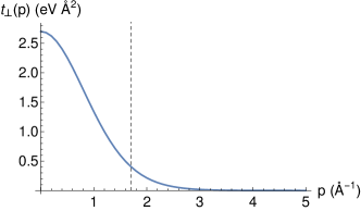
Figure 10: Fourier transform for the interlayer hopping in tBLG. The vertical dashed line marks the position of the Dirac point: $p=\left|\text{K}\right|$.

The fact that $t_{\perp}\left(\bm{p}\right)$ decays rapidly for large values of $\left|\bm{p}\right|$ has important consequences, as it means that only a few umklapp processes contribute significantly to the interlayer coupling.

III.2.4 Interlayer Hamiltonian for small twist angles

We now wish to specialize to the case of tBLG in the limit of small twist angles. For small $\theta$, the Dirac points $\text{K}_{1}$ and $\text{K}_{2}$ are close to each other and we can neglect coupling between $\text{K}_{\ell}$ and $-\text{K}_{\ell}$ points. If we are only interested in low-energy physics we can expand all quantities around these points. Therefore, close to the $\text{K}_{\ell}$ points, we can write

$$\bm{k}_{\ell}=\text{K}_{\ell}+\bm{q}_{\ell}.$$ (78)

As a result, the interlayer coupling, Eq. (70), becomes

$$T_{12}^{\alpha\beta}\left(\bm{q}_{1},\bm{q}_{2}\right)=\frac{1}{A_{u.c.}}\sum_{\bm{G}_{1},\bm{G}_{2}}e^{-i\bm{G}_{1}\cdot\bm{\tau}_{1,\alpha}}t_{12}^{\alpha\beta}\left(\text{K}_{1}+\bm{q}_{1}+\bm{G}_{1}\right)e^{-i\bm{G}_{2}\cdot\bm{\tau}_{2,\beta}}\delta_{\text{K}_{1}+\bm{q}_{1}+\bm{G}_{1},\text{K}_{2}+\bm{q}_{2}+\bm{G}_{2}}.$$ (79)

For states close to the Dirac points, we have $\left|\bm{q}_{1}\right|,\left|\bm{q}_{2}\right|\ll\left|\text{K}\right|$, and we can approximate $t_{\perp}\left(\text{K}_{1}+\bm{q}_{1}+\bm{G}_{1}\right)\simeq t_{\perp}\left(\text{K}_{1}+\bm{G}_{1}\right)$. As previously discussed, $t_{\perp}\left(\bm{p}\right)$ decays rapidly as a function of $\left|\bm{p}\right|$ and we can thus keep only the three most relevant processes, which correspond to interlayer hopping terms with momentum close to the three equivalent Dirac points. Therefore, we restrict the sum to $\bm{G}_{\ell}=\bm{g}_{\ell,1},\,\bm{g}_{\ell,2},\,\bm{g}_{\ell,3}$, with $\bm{g}_{\ell,1}=\bm{0}$, $\bm{g}_{\ell,2}=\bm{b}_{\ell,2}$ and $\bm{g}_{\ell,3}=-\bm{b}_{\ell,1}$. This leads to

$$T_{12}^{\alpha\beta}\left(\bm{q}_{1},\bm{q}_{2}\right)=T_{\bm{q}_{b}}^{\alpha\beta}\delta_{\bm{q}_{1}-\bm{q}_{2},-\bm{q}_{b}}+T_{\bm{q}_{tr}}^{\alpha\beta}\delta_{\bm{q}_{1}-\bm{q}_{2},-\bm{q}_{tr}}+T_{\bm{q}_{tl}}^{\alpha\beta}\delta_{\bm{q}_{1}-\bm{q}_{2},-\bm{q}_{tl}},$$ (80)

where we used that fact that $\left|\text{K}_{1}+\bm{g}_{1,n}\right|=\left|\text{K}\right|=4\pi/\left(3a\right)$ for $n=1(b),2(tr),3(tl)$. In the above equation, we have defined $T_{\boldsymbol{q}_{n}}^{\alpha\beta}=\frac{t_{\perp}\left(\left|\text{K}\right|\right)}{A_{u.c.}}e^{i\bm{g}_{1,n}\cdot\bm{\tau}_{1,\alpha}}e^{-i\bm{g}_{2,n}\cdot\bm{\tau}_{2,\beta}}$, which, in the $A,B$ basis, can be written in the following matrix form:

$$T_{\bm{q}_{b}} =\frac{t_{\perp}\left(\left|\text{K}\right|\right)}{A_{u.c.}}\left[\begin{array}[]{cc}1&1\\ 1&1\end{array}\right],$$ (83)

$$T_{\bm{q}_{tr}} =\frac{t_{\perp}\left(\left|\text{K}\right|\right)}{A_{u.c.}}e^{-i\bm{g}_{1,2}\cdot\bm{\tau}_{0}}\left[\begin{array}[]{cc}e^{i\phi}&1\\ e^{-i\phi}&e^{i\phi}\end{array}\right],$$ (86)

$$T_{\bm{q}_{tl}} =\frac{t_{\perp}\left(\left|\text{K}\right|\right)}{A_{u.c.}}e^{-i\bm{g}_{1,3}\cdot\bm{\tau}_{0}}\left[\begin{array}[]{cc}e^{-i\phi}&1\\ e^{i\phi}&e^{-i\phi}\end{array}\right],$$ (89)

with $\phi=2\pi/3$. In addition, we have also introduced the vectors

$$\bm{q}_{b} =\text{K}_{1}-\text{K}_{2},$$ (90)

$$\bm{q}_{tr} =\text{K}_{1}+\bm{g}_{1,2}-\text{K}_{2}-\bm{g}_{2,2},$$ (91)

$$\bm{q}_{tl} =\text{K}_{1}+\bm{g}_{1,3}-\text{K}_{2}-\bm{g}_{2,3}.$$ (92)

In the coordinate system where layer $2$ is rotated by $\theta/2$ and layer $1$ by $-\theta/2$, these three vectors are given explicitly given by

$$\bm{q}_{b} =\left|\Delta\text{K}\right|\left(0,-1\right),$$ (93)

$$\bm{q}_{tr} =\left|\Delta\text{K}\right|\left(\frac{\sqrt{3}}{2},\frac{1}{2}\right),$$ (94)

$$\bm{q}_{tl} =\left|\Delta\text{K}\right|\left(-\frac{\sqrt{3}}{2},\frac{1}{2}\right).$$ (95)

In Fig. 11, we represent the different transfered momenta in reciprocal space.

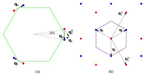
Figure 11: Momentum-space geometrical picture for the interlayer hopping on a tBLG. (a) The green dashed line marks the first BZ for an unrotated SLG; the red (blue) circles mark the three equivalent Dirac points for layer 1 (2). States from both layers couple when $\bm{q}_{2}-\bm{q}_{1}=\bm{q}_{b},\bm{q}_{tr},\bm{q}_{tl}$. (b) The three equivalent Dirac points in the first BZ result in three distinct hopping processes in reciprocal space; when we capture processes to all orders in the interlayer hopping, but considering only the transference of momentum by $\bm{q}_{b},\bm{q}_{tr},\bm{q}_{tl}$, we obtain this $\bm{k}$-space honeycomb structure, which captures the periodicity of the moiré pattern. The purple dashed line marks a moiré unit cell in reciprocal space.

The interlayer hopping from layer $2$ to layer $1$ can be obtained from the hermitian conjugate of Eq. (80),

$$T_{21}^{\alpha\beta}\left(\bm{q}_{2},\bm{q}_{1}\right)=\left(T_{\bm{q}_{b}}^{\beta\alpha}\right)^{*}\delta_{\bm{q}_{2}-\bm{q}_{1},\bm{q}_{b}}+\left(T_{\bm{q}_{tr}}^{\beta\alpha}\right)^{*}\delta_{\bm{q}_{2}-\bm{q}_{1},\bm{q}_{tr}}+\left(T_{\bm{q}_{tl}}^{\beta\alpha}\right)^{*}\delta_{\bm{q}_{2}-\bm{q}_{1},\bm{q}_{tl}}.$$ (96)

If we set $\theta=0$ and $\bm{\tau}_{0}=\bm{0}$, we recover Bernal-stacked BLG, with the interlayer coupling given by

$$T_{12}^{\alpha\beta}\left(\bm{q}_{2},\bm{q}_{1}\right)=\frac{t_{\perp}\left(\left|\text{K}\right|\right)}{A_{u.c.}}\left\{\left[\begin{array}[]{cc}1&1\\ 1&1\end{array}\right]+\left[\begin{array}[]{cc}e^{i\phi}&1\\ e^{-i\phi}&e^{i\phi}\end{array}\right]+\left[\begin{array}[]{cc}e^{-i\phi}&1\\ e^{i\phi}&e^{-i\phi}\end{array}\right]\right\}=\frac{3t_{\perp}\left(\left|\text{K}\right|\right)}{A_{u.c.}}\left[\begin{array}[]{cc}0&1\\ 0&0\end{array}\right].$$ (97)

Comparing Eq. (97) with the Hamiltonian for Bernal-stacked BLG, Eq. (42), we get

$$t_{\perp}=\frac{3t_{\perp}\left(\left|\text{K}\right|\right)}{A_{u.c.}}.$$ (98)

This relation fixes the value of $t_{\perp}(K)$ as

$$t_{\perp}\left(\left|\text{K}\right|\right)\simeq 0.58$\mathrm{eV}\text{\,}{\mathrm{\SIUnitSymbolAngstrom}}^{2}$,$$ (99)

which is, to a good approximation, consistent with the result obtained by the numerical calculation (Fig. 10).

The derivation of the interlayer coupling for states close to the $-\text{K}_{\ell}$ points expansion is completely analogous to the $+\text{K}_{\ell}$ case. Therefore, we just present the final result, which reads as

$$\tilde{T}_{12}^{\alpha\beta}\left(\bm{q}_{1},\bm{q}_{2}\right)=\tilde{T}_{\boldsymbol{q}_{b}}^{\alpha\beta}\delta_{\bm{q}_{1}-\bm{q}_{2},\bm{q}_{b}}+\tilde{T}_{\boldsymbol{q}_{tr}}^{\alpha\beta}\delta_{\bm{q}_{1}-\bm{q}_{2},\bm{q}_{tr}}+\tilde{T}_{\boldsymbol{q}_{tl}}^{\alpha\beta}\delta_{\bm{q}_{1}-\bm{q}_{2},\bm{q}_{tl}},$$ (100)

with

$$\tilde{T}_{\boldsymbol{q}_{b}} =\frac{t_{\perp}\left(\left|\text{K}\right|\right)}{A_{u.c.}}\left[\begin{array}[]{cc}1&1\\ 1&1\end{array}\right],$$ (103)

$$\tilde{T}_{\boldsymbol{q}_{tr}} =\frac{t_{\perp}\left(\left|\text{K}\right|\right)}{A_{u.c.}}e^{i\bm{g}_{1,2}\cdot\bm{\tau}_{0}}\left[\begin{array}[]{cc}e^{-i\phi}&1\\ e^{i\phi}&e^{-i\phi}\end{array}\right],$$ (106)

$$\tilde{T}_{\boldsymbol{q}_{tl}} =\frac{t_{\perp}\left(\left|\text{K}\right|\right)}{A_{u.c.}}e^{i\bm{g}_{1,3}\cdot\bm{\tau}_{0}}\left[\begin{array}[]{cc}e^{i\phi}&1\\ e^{-i\phi}&e^{i\phi}\end{array}\right].$$ (109)

III.3 Electronic properties

Having obtained a model Hamiltonian capable of describing tBLG, we will now analyze how the dispersion relation of electrons is affected by the interlayer coupling.

III.3.1 Renormalization of the Fermi velocity

We start by studying perturbatively the effect of interlayer coupling to states close to the Dirac points of one layer. Let us consider a state of layer $1$, with crystal-momentum $\text{K}_{1}+\bm{q}$. According to Eq. (80), this state will couple to states of layer $2$ with crystal momentum $\text{K}_{2}+\bm{q}_{2}$, with three possibilities for $\boldsymbol{q}_{2}$:

$$\bm{q}_{2} =\bm{q}+\bm{q}_{b},\quad\bm{q}_{2}=\bm{q}+\bm{q}_{tr},\quad\text{or}\quad\bm{q}_{2}=\bm{q}+\bm{q}_{tl}.$$ (110)

Considering only these states, we can build the following truncated Hamiltonian matrix:

$$H_{4,\text{tBLG}}^{\text{K}}(\bm{q})=\begin{bmatrix}H_{1}^{\text{K}}(\bm{q})&T_{\bm{q}_{b}}&T_{\bm{q}_{tr}}&T_{\bm{q}_{tl}}\\ T_{\bm{q}_{b}}^{\dagger}&H_{2}^{\text{K}}(\bm{q}+\bm{q}_{b})&0&0\\ T_{\bm{q}_{tr}}^{\dagger}&0&H_{2}^{\text{K}}(\bm{q}+\bm{q}_{tr})&0\\ T_{\bm{q}_{tl}}^{\dagger}&0&0&H_{2}^{\text{K}}(\bm{q}+\bm{q}_{tl})\end{bmatrix},$$ (111)

which is written in the basis $\left|1,\text{K}_{1}+\bm{q},\alpha\right\rangle$, $\left|2,\text{K}_{2}+\bm{q}+\bm{q}_{b},\alpha\right\rangle$, $\left|2,\text{K}_{2}+\bm{q}+\bm{q}_{tr},\alpha\right\rangle$, $\left|2,\text{K}_{2}+\bm{q}+\bm{q}_{tl},\alpha\right\rangle$.

If $\left|\bm{q}\right|\ll\left|\bm{q}_{n}\right|$ and $t_{\perp}\ll v_{F}\hbar\left|\bm{q}_{n}\right|$, we can integrate out the states from layer $2$ and obtain an effective Hamiltonian for layer 1. By doing so, we get

$$H_{1,\text{eff}}^{\text{K}}(\bm{q})=H_{1}^{\text{K}}(\bm{q})-\sum_{n=1}^{3}T_{\boldsymbol{q}_{n}}\cdot\left[H_{2}^{\text{K}}(\bm{q}+\bm{q}_{n})\right]^{-1}\cdot T_{\boldsymbol{q}_{n}}^{\dagger}.$$ (112)

From Eq. (58), it is straightforward to see that $\left[H_{2}^{\text{K}}(\bm{q})\right]^{-1}=\left(\bm{\sigma}^{\theta}\cdot\bm{q}\right)/\left(v_{F}\hbar\left|\bm{q}\right|^{2}\right)$. Expanding to lowest order in $\bm{q}$, we obtain

$$H_{1,\text{eff}}^{\text{K}}(\bm{q})=H_{1}^{\text{K}}(\bm{q})-\frac{1}{v_{F}\hbar\left|\Delta\text{K}\right|^{2}}\sum_{n=1}^{3}\left[T_{\boldsymbol{q}_{n}}\cdot\bm{\sigma}^{\theta}\cdot T_{\boldsymbol{q}_{n}}^{\dagger}\right]\cdot\left(\bm{q}-\bm{q}_{n}+2\bm{q}_{n}\frac{\bm{q}_{n}\cdot\bm{q}}{\bm{q}_{n}^{2}}\right).$$ (113)

Performing the sum over $\bm{q}_{n}$, we get

$$H_{1,\text{eff}}^{\text{K}}(\bm{q})=v_{F}\hbar\left(1-9\alpha^{2}\right)\left[\begin{array}[]{cc}0&q_{x}-iq_{y}\\ q_{x}+iq_{y}&0\end{array}\right]-6v_{F}\hbar\left|\Delta\text{K}\right|\sin\left(\frac{\theta}{2}\right)\alpha^{2}\left[\begin{array}[]{cc}1&0\\ 0&1\end{array}\right],$$ (114)

where $\alpha=t_{\perp}\left(\left|\text{K}\right|\right)/\left(v_{F}\hbar\left|\Delta\text{K}\right|A_{u.c.}\right)$. The second term in Eq. (114) is just a shift in the zero of energy. The first term leads to a renormalization of the Fermi velocity (Santos2007, ),

$$\frac{v_{F}^{*}(\theta)}{v_{F}}=1-\left(\frac{t_{\perp}\left(\left|\text{K}\right|\right)}{v_{F}\hbar\left|\text{K}\right|A_{u.c.}}\right)^{2}\frac{1}{4\sin^{2}\left(\theta/2\right)},$$ (115)

which shows that, depending on the twist angle, the effective Fermi velocity can take significantly smaller values. Notice that for small angles, the Fermi velocity can actually become zero. Clearly, for very small angles we can no longer assume that $t_{\perp}\ll v_{F}\hbar\left|\bm{q}_{n}\right|$, and the perturbative approach breaks down. However, it is true that at certain “magic angles” (which occur for $\theta\lesssim 1.05^{\circ}$) the Fermi velocity does vanish and flat bands appear at the Fermi level of tBLG (Bistritzer2011, ).

III.3.2 Band structure, density of states and carrier density profile

In order to obtain an accurate description of the electronic properties of tBLG, we must go beyond the perturbative approach previously described. To do so, we must go beyond the truncation employed in the Hamiltonian of Eq. (111). This Hamiltonian does not include the fact that each of the states $\left|2,\text{K}_{2}+\bm{q}+\bm{q}_{n},\alpha\right\rangle$ of layer $2$ is also coupled to several states of layer $1$, as described by Eq. (96), and so on, for increasing truncation orders.

It is worth noticing that the three transfered momenta in the interlayer hopping, Eqs. (90)-(92), can be written as

$$\bm{q}_{b}=\Delta\text{K},\quad\bm{q}_{tr}=\Delta\text{K}+\bm{b}_{2}^{m},\quad\bm{q}_{tl}=\Delta\text{K}-\bm{b}_{1}^{m},$$ (116)

which tells us that, in the interlayer hopping, there is a transference of momentum by reciprocal lattice vectors of the moiré pattern. This motivates us to look for eigenstates of the tBLG structure of the form

$$\left|\psi_{\bm{q}}^{m}\right\rangle=\sum_{\ell,\alpha,m_{1},m_{2}}u_{\alpha}^{(\ell)}\left(\bm{q},m_{1},m_{2}\right)\left|\ell,\bm{q},\left(m_{1},m_{2}\right),\alpha\right\rangle,$$ (117)

where we defined

$$\left|\ell,\bm{q},\left(m_{1},m_{2}\right),\alpha\right\rangle\equiv\left|\ell,\text{K}_{\ell}+\bm{q}+m_{1}\bm{b}_{1}^{m}+m_{2}\bm{b}_{2}^{m},\alpha\right\rangle.$$ (118)

For example, if we consider the states (we will drop the crystal-momenta $\bm{q}$ and the sublattice index $\alpha$ for simplicity) $\left|1,\left(0,0\right)\right\rangle,\,\left|2,(0,0)\right\rangle,\,\left|2,(0,1)\right\rangle\,\left|2,(-1,0)\right\rangle,\,\left|1,\left(0,-1\right)\right\rangle,\,\left|1,\left(1,0\right)\right\rangle,\,\left|1,\left(0,1\right)\right\rangle,\,\left|1,\left(1,1\right)\right\rangle,\,\left|1,\left(-1,0\right)\right\rangle,\,\left|1,\left(-1,-1\right)\right\rangle$, we obtain the following matrix:

$$H_{10,\text{tBLG}}^{\text{K}}(\bm{q})=\left[\begin{array}[]{cccccccccc}H_{1}^{\text{K}}&T_{\bm{q}_{b}}&T_{\bm{q}_{tr}}&T_{\bm{q}_{tl}}&0&0&0&0&0&0\\ T_{\bm{q}_{b}}^{\dagger}&H_{2}^{\text{K}}&0&0&T_{\bm{q}_{tr}}^{\dagger}&T_{\bm{q}_{tl}}^{\dagger}&0&0&0&0\\ T_{\bm{q}_{tr}}^{\dagger}&0&H_{2}^{\text{K}}&0&0&0&T_{\bm{q}_{b}}^{\dagger}&T_{\bm{q}_{tl}}^{\dagger}&0&0\\ T_{\bm{q}_{tl}}^{\dagger}&0&0&H_{2}^{\text{K}}&0&0&0&0&T_{\bm{q}_{b}}^{\dagger}&T_{\bm{q}_{tr}}^{\dagger}\\ 0&T_{\bm{q}_{tr}}&0&0&H_{1}^{\text{K}}&0&0&0&0&0\\ 0&T_{\bm{q}_{tl}}&0&0&0&H_{1}^{\text{K}}&0&0&0&0\\ 0&0&T_{\bm{q}_{b}}&0&0&0&H_{1}^{\text{K}}&0&0&0\\ 0&0&T_{\bm{q}_{tl}}&0&0&0&0&H_{1}^{\text{K}}&0&0\\ 0&0&0&T_{\bm{q}_{b}}&0&0&0&0&H_{1}^{\text{K}}&0\\ 0&0&0&T_{\bm{q}_{tr}}&0&0&0&0&0&H_{1}^{\text{K}}\end{array}\right],$$ (119)

where for compactness we have also suppressed the momenta argument of $H_{1/2}^{\text{K}}$, which should read as $\bm{q}+m_{1}\bm{b}_{1}^{m}+m_{2}\bm{b}_{2}^{m}$ for $H_{1}^{\text{K}}$ and $\bm{q}+\bm{q}_{b}+m_{1}\bm{b}_{1}^{m}+m_{2}\bm{b}_{2}^{m}$ for $H_{2}^{\text{K}}$. By computing the eigenvalues of $H_{10,\text{tBLG}}^{\text{K}}(\bm{q})$ we obtain an approximation for the electronic band structure in the moiré BZ. The index $10$ means that we are considering ten moiré reciprocal lattice vectors, which due to the sublattice degree of freedom, implies that $H_{10,\text{tBLG}}^{\text{K}}(\bm{q})$ is a $20\times 20$ matrix. By considering more and more moiré reciprocal lattice vectors, this approximation can be improved. In this matrix construction, we point out the similarities with what we have shown for the folded band description of SLG in section II.1.4. In fact, if we disregard the interlayer (off-diagonal) hopping terms, we see that we are basically using a folded band description that explicitly captures the moiré periodicity to some extent (depending on the truncation order). In real space, this corresponds to take an enlarged unit cell with the moiré periodicity.

Results for the electronic spectrum and the DOS, taking contributions from states close to K and $\text{K}^{\prime}$, are shown in Fig. 12. We show how both K and $\text{K}^{\prime}$ points are folded into the same moiré BZ in Fig. 13. It is apparent that, in a K expansion, the wave vector $\bm{q}$ is measured from $\text{K}_{1}$ ($\bm{k}=\text{K}_{1}+\bm{q}$) while, in a $\text{K}^{\prime}$ expansion, we measure it from $\text{K}_{1}^{\prime}$. Therefore, in order to match both moiré unit cells in reciprocal space (purple and green), we identify the points $\text{K}_{1}$ and $\text{K}_{2}^{\prime}$ as the same point in the moiré BZ, such that the paths $\text{K}_{m}\rightarrow\text{K}_{m}^{\prime}\rightarrow\text{M}_{m}\rightarrow\text{K}_{m}$ become equivalent. By doing so, we are making a correspondence $H^{\text{K}}(\bm{q})\leftrightarrow H^{\text{K}^{\prime}}(\bm{q}+\bm{q}_{b})$ in the Hamiltonians obtained within K and $\text{K}^{\prime}$ expansions.

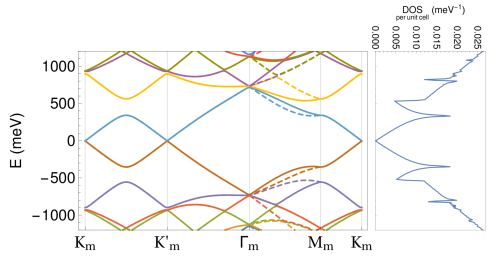
Figure 12: Electronic spectrum and DOS for tBLG with $\theta=5^{\circ}$. Solid and dashed lines in the spectrum are for K and $\text{K}^{\prime}$ expansions, respectively; the color code clarifies the situation in which K and $\text{K}^{\prime}$ bands are superimposed.

Figure 13: Picture of K and $\text{K}^{\prime}$ expansions on a tBLG. (a) Blue/red hexagons describe the BZs for layers 1/2. Dashed purple/green hexagons represent moiré unit cells in reciprocal space for K/$\text{K}^{\prime}$ expansions. (b) Moiré BZ with relevant points plotted in it.

Looking at the spectrum of Fig. 12, we see that a symmetry for positive and negative bands is apparently conserved. As predicted in the previous section, we also observe a renormalization of the Fermi velocity (Santos2007, ; Bistritzer2011, ). In addition, we verify the emergence of low energy van Hove singularities. These singularities are due to the avoided crossings of the Dirac cones of the two layers that occur at the middle point between $\text{K}_{1}$ and $\text{K}_{2}$. Therefore, it is possible to tune the position in energy of these van Hove singularities by varying the twist angle. In this chapter, we have avoided the so-called “magic angles” (Bistritzer2011, ), for which the Fermi velocity vanishes due to the merging of the two van Hove singularities.

The DOS and carrier density profile are plotted in Fig. 14 for different twist angles $\theta$. We confirm that, by varying the twist angle, van Hove singularities can be brought to experimentally accessible energies. As for the carrier density profile, we observe that we start to lose the signature behavior of the decoupled BLG —tBLG with $t_{\perp}=0$— when we approach small angles.

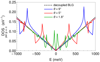
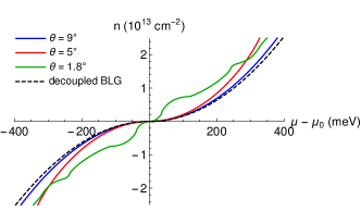
Figure 14: DOS and carrier density profile for different angles of a tBLG. Since the size of the unit cells varies with the angle, the DOS is normalized to the graphene unit cell (g.u.c.). $\mu_{0}$ is the Fermi level at half filling. Decoupled BLG corresponds to tBLG with $t_{\perp}=0$.

The method described in this section to evaluate the moiré band structure of tBLG is analogous to the plane-wave expansion of the form

$$\psi_{\bm{k},n}(\bm{r})=\sum_{\bm{G}}u_{\bm{k},n}\left(\bm{G}\right)e^{i\left(\bm{k}+\bm{G}\right)\cdot\bm{r}},$$ (120)

which can be used to determine the electronic spectrum of a periodic system with lattice $\left\{\bm{R}\right\}$ and reciprocal lattice $\left\{\bm{G}\right\}$. The main difference is that in the present case the expansion is made in terms of Bloch waves. There is, yet, another important difference. The plane-wave expansion in a periodic system, Eq. (120), always contains an infinite number of $\bm{G}$ vectors, which is then truncated, leading to electronic bands evaluated with a certain numerical precision. The expansion for tBLG in Eq. (117) can be either infinite or finite. For a commensurate system, there will be a certain $\bm{G}^{m}$ that coincides with a reciprocal lattice vector of both individual layers, such that an expansion of the form of Eq. (117) becomes finite. For an incommensurate structure there is never a $\bm{G}^{m}$ that coincides with reciprocal lattice vectors of both layers and therefore the expansion in Eq. (117) is formally infinite. This also has an important physical consequence. In a incommensurate structure, the electronic properties are independent of the in-plane translation $\bm{\tau}_{0}$. This can be seen by performing a unitary transformation in the basis states (Bistritzer2011, ; Koshino2015, ),

$$\left|\ell,\boldsymbol{q},(m_{1},m_{2}),\alpha\right\rangle\rightarrow e^{i\left(m_{1}\boldsymbol{b}_{1,1}+m_{2}\boldsymbol{b}_{1,2}\right)\cdot\bm{\tau}_{0}}\left|\ell,\boldsymbol{q},(m_{1},m_{2}),\alpha\right\rangle,$$ (121)

which makes the Hamiltonians independent of $\bm{\tau}_{0}$ (check, for instance, the Hamiltonian of Eq. (119)), allowing us to set $\bm{\tau}_{0}=\bm{0}$ without any loss of generality. Such transformation does not eliminate the $\bm{\tau}_{0}$ dependency in a commensurate structure, as can be easily understood by comparing the Hamiltonians for AA and AB stacked BLG.

Finally, we finish with a discussion about the validity of the model. The leading corrections involve hopping amplitudes that, due to the momentum conservation $\text{K}_{1}+\bm{q}_{1}+\bm{G}_{1}=\text{K}_{2}+\bm{q}_{2}+\bm{G}_{2}$, are negligible when compared to $t_{\perp}(\left|\text{K}\right|)$. We should also not forget that we are using a Dirac approximation for the individual layers. Therefore, we expect our model to be accurate up to energies of $\sim 1$\mathrm{eV}$$, which can still capture the first low-energy bands for $\theta\lesssim 10^{\circ}$. In case of larger angles, it is still possible (Koshino2015, ) to apply the same technology presented here, but one must consider the general form of the interlayer coupling, Eq. (70), and the full tight-binding Hamiltonian of the individual layers, Eq. (56).

IV Optical response

The study of light-matter interactions is a topic of interest in science, with a wide variety of applications, for example in the field of photonics. For the tBLG system, the response to an applied electromagnetic field can be characterized by its optical conductivity, which has been measured experimentally (Wang2010, ; Zou2013, ; Cao2016, ). On the theoretical side, we highlight the following works: in Ref. (Tabert2013, ), the authors used the simplified model from Ref. (Gail2011, ) to study the dynamic (frequency dependent) conductivity at different levels of chemical potential; tight-binding-based calculations of the dynamic conductivity were performed by Moon and Koshino (Moon2013, ); the real and imaginary parts of the conductivity were calculated by Stauber et al. (Stauber2013, ), using a continuum low-energy model based on Refs. (Santos2007, ; Bistritzer2011, ).

Over the last few years, graphene plasmonics has emerged as a new research topic. Surface plasmon-polaritons (SPPs) are collective excitations of coupled charge density modulations and photons, which propagate along surfaces. The interest on plasmons in graphene picked up after the experimental excitation of graphene SPPs in the $\mathrm{THz}$ spectral range by Ju et al. in 2011 (Ju2011, ). The excitation of graphene SPPs was achieved by shining electromagnetic radiation onto a periodic grid of graphene micro-ribbons, in a way that the periodic grid provides the momentum that the light lacks for exciting the plasmons. Other methods of excitation are also possible, as the one depicted in Fig. 15, where a continuous graphene sheet is shined with light that goes through a metallic grid. Owing to the 2D nature of the collective excitations, graphene SPPs are confined much more strongly than those in conventional metals (particularly in the $\mathrm{THz}$ spectral range), making it a promising candidate for future applications (Jablan2009, ; Koppens2011, ; Luo2013, ). In addition, perhaps the most important advantage of using graphene is the tunability of the graphene SPPs, since carrier densities in graphene can be easily controlled by electrical gating and doping (Ju2011, ; Vakil2011, ; Fang2012, ; Fei2012, ; Chen2012, ; Grigorenko2012, ). As we will see, within the semi-classical model, the dispersion relation of SPPs in graphene depends explicitly on the optical conductivity, wherefore the study of their spectrum follows as a direct application. For an in-depth introduction to the field of plasmonics in graphene, we point the interested reader to Ref. (Goncalves2016, ).

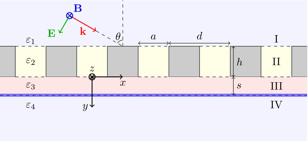
Figure 15: Possible scheme to excite SPPs in graphene: a graphene layer (blue line) is located between two dielectric media (III and IV), with a periodic grid of metallic micro-ribbons placed on top; the polarized light is shined from the outside (medium I). The periodic grid provides the momentum that is required to satisfty the energy-momentum conservation relation between the incident light and the excited SPP.

The goal of this section is to study the response of the tBLG system to an electromagnetic stimuli. We begin with the optical conductivity, which we evaluate having as a starting point the electronic Hamiltonian described in the previous section. Within the linear response theory, we take the velocity gauge Passos2018 and derive expressions that can be implemented when an analytical Hamiltonian matrix is known. As benchmark, we compute the results for the SLG; then, we apply the same method to the tBLG. Next, we study the dispersion relation of SPPs supported by tBLG. We consider few-layer graphene embedded in dielectric media and derive the equation that describes the propagation of transverse magnetic waves along the 2D surface, which depends on the dynamic conductivity. Again, we make the calculations for both the SLG and the tBLG. We point out that SPPs in tBLG were first studied by Stauber et al. (Stauber2013, ).

IV.1 Conductivity

IV.1.1 Linear response theory

General tight-binding description

We recall that the starting point of our description of tBLG was a tight-binding Hamiltonian, which in general can be written as in Eq. (5),

$$H=\sum_{\bm{R},\bm{\delta},\alpha,\beta}c_{\alpha}^{\dagger}\left(\bm{R}\right)h_{\bm{\delta}}^{\alpha\beta}c_{\beta}\left(\bm{R}+\bm{\delta}\right).$$ (122)

This Hamiltonian can be coupled to an external electromagnetic field using a minimal coupling approach (Doughty1990, ). For a tight-binding model, minimal coupling reduces to the Peierls substitution, where each hopping $h_{\bm{\delta}}^{\alpha\beta}$ is multiplied by the phase that the electron acquires when hopping from one atomic center to other. Therefore, the Hamiltonian becomes

$$H_{A}(t)=\sum_{\bm{R},\bm{\delta},\alpha,\beta}c_{\alpha}^{\dagger}\left(\bm{R}\right)\exp\left[-i\frac{e}{\hbar}\int_{\bm{R}+\bm{\delta}+\bm{\tau}_{\beta}}^{\bm{R}+\bm{\tau}_{\alpha}}d\bm{r}\cdot\bm{A}(\bm{r},t)\right]h_{\bm{\delta}}^{\alpha\beta}c_{\beta}\left(\bm{R}+\bm{\delta}\right),$$ (123)

where $\bm{A}(\bm{r},t)$ is the electromagnetic vector potential and $e>0$ is the elementary charge.

In the following, we will be interested in the response to homogeneous electromagnetic fields, for which the previous expression reduces to

$$H_{A}(t)=\sum_{\bm{R},\bm{\delta},\alpha,\beta}c_{\alpha}^{\dagger}\left(\bm{R}\right)\exp\left[-i\frac{e}{\hbar}\bm{A}(t)\cdot\left(\bm{\tau}_{\alpha}-\bm{\delta}-\bm{\tau}_{\beta}\right)\right]h_{\bm{\delta}}^{\alpha\beta}c_{\beta}\left(\bm{R}+\bm{\delta}\right).$$ (124)

Writing the fermionic operators according to Eq. (40),

$$c_{\alpha}^{\dagger}(\bm{R})=\frac{1}{\sqrt{N}}\sum_{\bm{k}}e^{-i\bm{k}\cdot\left(\bm{R}+\bm{\tau}_{\alpha}\right)}c_{\alpha}^{\dagger}(\bm{k}),$$ (125)

we get

$$H_{A}(t)=\sum_{\bm{k},\alpha,\beta}c_{\alpha}^{\dagger}\left(\bm{k}\right)h_{0}\left(\bm{k}+\frac{e}{\hbar}\bm{A}(t)\right)c_{\beta}\left(\bm{k}\right),$$ (126)

where $h_{0}\left(\bm{k}\right)=\sum_{\bm{\delta}}h_{\bm{\delta}}^{\alpha\beta}e^{i\bm{k}\cdot\left(\bm{\delta}+\bm{\tau}_{\beta}-\bm{\tau}_{\alpha}\right)}$ are the matrix elements of the reciprocal-space tight-binding Hamiltonian in the $\alpha,\beta$ basis. For SLG, $\alpha,\beta$ are sublattice indeces whereas, for Bernal-stacked BLG, they label both sublattice and layer. In the case of tBLG, $\alpha,\beta$ run over all the entries of matrices as the one shown in Eq. (119). In this case, we also have to separate the sum over $\boldsymbol{k}\in\text{BZ}$ into two sums over $\boldsymbol{q}$ in moiré BZs centered around K and $\text{K}^{\prime}$. Finally, we stress that, in the $\alpha,\beta$ basis, the Hamiltonians are not diagonal.

Perturbative treatment to the minimal coupling

Starting from the Hamiltonian given by Eq. (126) and expanding it in $\bm{A}(t)$, we obtain the standard description of an unperturbed Hamiltonian $H_{0}$ plus a time-dependent perturbation $V(t)$,

$$H_{A}(t)=H_{0}+V(t),$$ (127)

with

$$H_{0}=\sum_{\bm{k},\alpha,\beta}c_{\alpha}^{\dagger}\left(\bm{k}\right)h_{0}\left(\bm{k}\right)c_{\beta}\left(\bm{k}\right),$$ (128)

$$V(t)=\sum_{\bm{k},\alpha,\beta}\left(\frac{e}{\hbar}\frac{\partial h_{0}(\bm{k})}{\partial k_{a_{1}}}A_{a_{1}}(t)+\frac{1}{2!}\left(\frac{e}{\hbar}\right)^{2}\frac{\partial^{2}h_{0}(\bm{k})}{\partial k_{a_{1}}\partial k_{a_{2}}}A_{a_{1}}(t)A_{a_{2}}(t)+...\right)c_{\bm{k},\alpha}^{\dagger}c_{\bm{k},\beta}.$$ (129)

In the equation above, we clarify that we are using Einstein’s summation convention for the mute indices $a_{i}=x,y$. It must also be noted that, in the Dirac approximation for graphene, only the first term is non-zero. However, for a general tight-binding Hamiltonian, terms to all orders in $\bm{A}(t)$ exist.

The homogenous 2D current density operator can be obtained as

$$J_{a_{1}}(t)=-\frac{1}{A}\frac{\partial H_{A}(t)}{\partial A_{a_{1}}}=-\frac{e}{\hbar A}\sum\limits_{\bm{k},\alpha,\beta}\left(\frac{\partial h_{0}(\bm{k})}{\partial k_{a_{1}}}+\frac{e}{\hbar}\frac{\partial^{2}h_{0}(\bm{k})}{\partial k_{a_{1}}\partial k_{a_{2}}}A_{a_{2}}(t)+...\right)c_{\bm{k},\alpha}^{\dagger}c_{\bm{k},\beta},$$ (130)

where $A$ is the area of the 2D system. Using the time-dependent perturbation theory in the interaction representation, we get, for the average current density,

$$\left\langle J_{a_{1}}^{I}(t)\right\rangle= \left\langle J_{a_{1}}^{I}(t)\right\rangle_{0}+\left(-\frac{i}{\hbar}\right)\int_{t_{0}}^{t}dt_{1}\left\langle\left[J_{a_{1}}^{I}(t),V_{I}(t_{1})\right]\right\rangle_{0}$$

$$+\left(-\frac{i}{\hbar}\right)^{2}\int_{t_{0}}^{t}dt_{1}\int_{t_{0}}^{t_{1}}dt_{2}\left\langle\left[\left[J_{a_{1}}^{I}(t),V_{I}(t_{1})\right],V_{I}(t_{2})\right]\right\rangle_{0}+...\quad,$$ (131)

where $\left\langle\ \right\rangle_{0}$ represents a thermal average over unperturbed states. Here, we are assuming that the initial condition of our system ($t=t_{0})$ is a thermal state of the unperturbed Hamiltonian $H_{0}$.

We now want to write Eqs. (129) and (130) in the interaction picture. First, we change to the basis $\left|\lambda\right\rangle$, which diagonalizes $H_{0}(\bm{k})$ with eigenvalues $\epsilon_{\lambda}(\boldsymbol{k})=\hbar\omega_{\lambda}$ (where we have omitted the momentum dependency of the angular frequencies $\omega_{\lambda}$), and write the fermionic operators in the interaction picture as

$$c_{\bm{k},\alpha}=\sum\limits_{\lambda}\left\langle\alpha|\lambda\right\rangle e^{-i\omega_{\lambda}(t-t_{0})}c_{\bm{k},\lambda},\quad c_{\bm{k},\alpha}^{\dagger}=\sum\limits_{\lambda}\left\langle\lambda|\alpha\right\rangle e^{i\omega_{\lambda}(t-t_{0})}c_{\bm{k},\lambda}^{\dagger}.$$ (132)

Then, we plug Eq. (132) into Eqs. (129) and (130) and, using the closure relation, $\sum\limits_{\gamma}\left|\gamma\right\rangle\left\langle\gamma\right|=1$, we obtain

$$V_{I}(t)=\sum\limits_{\bm{k},\lambda,\lambda^{\prime}}\left\langle\lambda\right|\left(\frac{e}{\hbar}\frac{\partial h_{0}(\bm{k})}{\partial k_{a_{1}}}A_{a_{1}}(t)+\frac{1}{2!}\left(\frac{e}{\hbar}\right)^{2}\frac{\partial^{2}h_{0}(\bm{k})}{\partial k_{a_{1}}\partial k_{a_{2}}}A_{a_{1}}(t)A_{a_{2}}(t)+...\right)\left|\lambda^{\prime}\right\rangle e^{i\omega_{\lambda\lambda^{\prime}}(t-t_{0})}c_{\bm{k},\lambda}^{\dagger}c_{\bm{k},\lambda^{\prime}},$$ (133)

$$J_{a_{1}}^{I}(t)=-\frac{e}{\hbar A}\sum\limits_{\bm{k},\lambda,\lambda^{\prime}}\left\langle\lambda\right|\left(\frac{\partial h_{0}(\bm{k})}{\partial k_{a_{1}}}+\frac{e}{\hbar}\frac{\partial^{2}h_{0}(\bm{k})}{\partial k_{a_{1}}\partial k_{a_{2}}}A_{a_{2}}(t)+...\right)\left|\lambda^{\prime}\right\rangle e^{i\omega_{\lambda\lambda^{\prime}}(t-t_{0})}c_{\bm{k},\lambda}^{\dagger}c_{\bm{k},\lambda^{\prime}},$$ (134)

where we have defined $\omega_{\lambda\lambda^{\prime}}=\omega_{\lambda}-\omega_{\lambda^{\prime}}$.

Equilibrium current

Collecting the zeroth-order terms (in the fields) from the average current, Eq. (131), we obtain the so-called equilibrium current,

$$J_{a_{1}}^{0}(t)=-\frac{e}{\hbar A}\sum_{\bm{k},\lambda,\lambda^{\prime}}\left\langle\lambda\left|\frac{\partial h_{0}(\bm{k})}{\partial k_{a_{1}}}\right|\lambda^{\prime}\right\rangle e^{i\omega_{\lambda\lambda^{\prime}}(t-t_{0})}\left\langle c_{\bm{k},\lambda}^{\dagger}c_{\bm{k},\lambda^{\prime}}\right\rangle_{0}.$$ (135)

In the equation above, the thermal average is trivially computed as $\left\langle c_{\bm{k},\lambda}^{\dagger}c_{\bm{k},\lambda^{\prime}}\right\rangle_{0}=\delta_{\lambda,\lambda^{\prime}}\ n_{F}\left(\epsilon_{\lambda}(\bm{k})\right)$, where $n_{F}$ stands for the Fermi-Dirac function, $n_{F}\left(\epsilon\right)=\left(e^{\frac{\epsilon-\mu}{k_{B}T}}+1\right)^{-1}$, in which $k_{B}$ is the Boltzmann constant, $T$ is the absolute temperature and $\mu$ is the Fermi level.

Taking into account the time inversion symmetry in reciprocal space, we can show that the equilibrium current is zero, $J_{a_{1}}^{0}(t)=0$. We point out that, even in our model for the tBLG, time inversion symmetry is not broken: we can explicitly see that, for every point $\bm{q}$ in the moiré BZ centered around K ($\bm{k}=\text{K}+\bm{q}$), we have a completely equivalent point $-\bm{k}=-\text{K}-\bm{q}$, which corresponds to a point $-\bm{q}$ in the moiré BZ centered around $\text{K}^{\prime}=-\text{K}$.

Linear response current and conductivity

We now collect the first order terms, which lead to the following linear response current:

$$J_{a_{1}}^{1}(t)= -\frac{e^{2}}{\hbar^{2}A}\sum\limits_{\bm{k},\lambda,\lambda^{\prime}}\left\langle\lambda\left|\frac{\partial^{2}h_{0}}{\partial k_{a_{1}}\partial k_{a_{2}}}\right|\lambda^{\prime}\right\rangle A_{a_{2}}(t)e^{i\omega_{\lambda\lambda^{\prime}}(t-t_{0})}\left\langle c_{\bm{k},\lambda}^{\dagger}c_{\bm{k},\lambda^{\prime}}\right\rangle_{0}$$

$$+\frac{ie^{2}}{\hbar^{3}A}\sum\limits_{\bm{k},\lambda_{1},\lambda_{2}}\sum\limits_{\bm{k}^{\prime},\lambda_{3},\lambda_{4}}\left\langle\lambda_{1}\left|\frac{\partial h_{0}}{\partial k_{a_{1}}}\right|\lambda_{2}\right\rangle\left\langle\lambda_{3}\left|\frac{\partial h_{0}}{\partial k_{a_{2}}^{\prime}}\right|\lambda_{4}\right\rangle\left\langle\left[c_{\bm{k},\lambda_{1}}^{\dagger}c_{\bm{k},\lambda_{2}}\ ,\ c_{\bm{k}^{\prime},\lambda_{3}}^{\dagger}c_{\bm{k}^{\prime},\lambda_{4}}\right]\right\rangle_{0}\times$$

$$\times\int_{t_{0}}^{t}dt_{1}\ e^{i\omega_{\lambda_{1}\lambda_{2}}(t-t_{0})}e^{i\omega_{\lambda_{3}\lambda_{4}}(t_{1}-t_{0})}A_{a_{2}}(t_{1}),$$ (136)

where, for simplicity, we have supressed the momentum argument in $h_{0}$.

Using the fermionic commutation relations, we obtain

$$\left\langle\left[c_{\bm{k},\lambda_{1}}^{\dagger}c_{\bm{k},\lambda_{2}}\ ,\ c_{\bm{k}^{\prime},\lambda_{3}}^{\dagger}c_{\bm{k}^{\prime},\lambda_{4}}\right]\right\rangle_{0}=\delta_{\bm{k},\bm{k}^{\prime}}\delta_{\lambda_{1},\lambda_{4}}\delta_{\lambda_{2},\lambda_{3}}\left(n_{F}(\epsilon_{\lambda_{1}})-n_{F}(\epsilon_{\lambda_{2}})\right),$$

where we have also omitted the momentum dependency of the eigenvalues, and use this to simplify Eq. (136) into

$$J_{a_{1}}^{1}(t)= -\frac{e^{2}}{\hbar^{2}A}\sum\limits_{\bm{k},\lambda}\left\langle\lambda\left|\frac{\partial^{2}h_{0}}{\partial k_{a_{1}}\partial k_{a_{2}}}\right|\lambda\right\rangle n_{F}(\epsilon_{\lambda})A_{a_{2}}(t)\$$

$$+\frac{ie^{2}}{\hbar^{3}A}\sum\limits_{\bm{k},\lambda_{1},\lambda_{2}}\left\langle\lambda_{1}\left|\frac{\partial h_{0}}{\partial k_{a_{1}}}\right|\lambda_{2}\right\rangle\left\langle\lambda_{2}\left|\frac{\partial h_{0}}{\partial k_{a_{2}}}\right|\lambda_{1}\right\rangle\left(n_{F}(\epsilon_{\lambda_{1}})-n_{F}(\epsilon_{\lambda_{2}})\right)\int_{t_{0}}^{t}dt_{1}\ e^{i\omega_{\lambda_{1}\lambda_{2}}(t-t_{1})}A_{a_{2}}(t_{1}).$$ (137)

At this point, we apply a Fourier transform to the magnetic vector potential,

$$A_{a}(t)=\int_{\mathbb{R}}\frac{d\omega}{2\pi}A_{a}(\omega)e^{-i\omega t},$$ (138)

where $\omega$ is the angular frequency of the light, and use the relation between the Fourier amplitude of the magnetic vector potential, $A_{a}(\omega)$, and the Fourier amplitude of the electric field, $E_{a}(\omega)$,

$$A_{a}(\omega)=\frac{E_{a}(\omega)}{i\omega},$$ (139)

to obtain

$$A_{a}(t)=\int_{\mathbb{R}}\frac{d\omega}{2\pi}\frac{E_{a}(\omega)}{i\omega}e^{-i\omega t},$$ (140)

where, in the adiabatic regime, we make $\omega\rightarrow\omega+i\gamma,\ \gamma\rightarrow 0^{+}$, meaning that we switch on the electromagnetic fields very slowly.

Substituting Eq. (140) into Eq. (137), we get

$$J_{a_{1}}^{1}(t)= \int_{\mathbb{R}}\frac{d\omega}{2\pi}\ \left(\frac{e^{2}}{\hbar^{2}A}\sum\limits_{\bm{k},\lambda}\left\langle\lambda\left|\frac{\partial^{2}h_{0}}{\partial k_{a_{1}}\partial k_{a_{2}}}\right|\lambda\right\rangle\frac{in_{F}(\epsilon_{\lambda})}{\omega}\right)E_{a_{2}}(\omega)e^{-i\omega t}$$

$$+\frac{ie^{2}}{\hbar^{3}A}\sum\limits_{\bm{k},\lambda_{1},\lambda_{2}}\left\langle\lambda_{1}\left|\frac{\partial h_{0}}{\partial k_{a_{1}}}\right|\lambda_{2}\right\rangle\left\langle\lambda_{2}\left|\frac{\partial h_{0}}{\partial k_{a_{2}}}\right|\lambda_{1}\right\rangle\left(n_{F}(\epsilon_{\lambda_{1}})-n_{F}(\epsilon_{\lambda_{2}})\right)\times$$

$$\times\int_{t_{0}}^{t}dt_{1}\ e^{i\omega_{\lambda_{1}\lambda_{2}}(t-t_{1})}\int_{\mathbb{R}}\frac{d\omega}{2\pi}\frac{E_{a_{2}}(\omega)}{i\omega}e^{-i\omega t_{1}}.$$ (141)

We can compute the integral in time,

$$\int_{t_{0}}^{t}dt_{1}\ e^{i\omega_{\lambda_{1}\lambda_{2}}(t-t_{1})}e^{-i\omega t_{1}}=e^{i\omega_{\lambda_{1}\lambda_{2}}t}\int_{t_{0}}^{t}dt_{1}\ e^{-i\left(\omega_{\lambda_{1}\lambda_{2}}+\omega\right)t_{1}}=\frac{ie^{-i\omega t}}{\omega_{\lambda_{1}\lambda_{2}}+\omega}+...,$$ (142)

where we have eliminated the last the term by making $t_{0}\rightarrow-\infty$, which means that we have waited long enough for the transient terms to be negligible. Using this result, we simplify the expression for the linear current density into

$$J_{a_{1}}^{1}(t)= \int_{\mathbb{R}}\frac{d\omega}{2\pi}\ \left(\frac{ie^{2}}{\hbar^{2}A}\sum\limits_{\bm{k},\lambda}\left\langle\lambda\left|\frac{\partial^{2}h_{0}}{\partial k_{a_{1}}\partial k_{a_{2}}}\right|\lambda\right\rangle\frac{n_{F}(\epsilon_{\lambda})}{\omega}\right)E_{a_{2}}(\omega)e^{-i\omega t}\$$

$$+\int_{\mathbb{R}}\frac{d\omega}{2\pi}\ \left(\frac{ie^{2}}{\hbar^{3}A}\sum\limits_{\bm{k},\lambda_{1},\lambda_{2}}\left\langle\lambda_{1}\left|\frac{\partial h_{0}}{\partial k_{a_{1}}}\right|\lambda_{2}\right\rangle\left\langle\lambda_{2}\left|\frac{\partial h_{0}}{\partial k_{a_{2}}}\right|\lambda_{1}\right\rangle\frac{n_{F}(\epsilon_{\lambda_{1}})-n_{F}(\epsilon_{\lambda_{2}})}{\omega(\omega_{\lambda_{1}\lambda_{2}}+\omega)}\right)E_{a_{2}}(\omega)e^{-i\omega t}.$$ (143)

Taking a closer look at the last expression, we identify the conductivity (rank-2) tensor, $\sigma$, which leads to the current that arises in response to an electric field ($\bm{J}=\sigma\bm{E}$ in matrix form), as

$$\sigma_{a_{1}a_{2}}(\omega)=\frac{i4\sigma_{0}}{NA_{u.c.}}\sum\limits_{\bm{k},\lambda_{1}}\left(\left\langle\lambda_{1}\left|\frac{\partial^{2}h_{0}}{\partial k_{a_{1}}\partial k_{a_{2}}}\right|\lambda_{1}\right\rangle\frac{n_{\lambda_{1}}^{F}}{\hbar\omega}+\sum\limits_{\lambda_{2}\neq\lambda_{1}}\left\langle\lambda_{1}\left|\frac{\partial h_{0}}{\partial k_{a_{1}}}\right|\lambda_{2}\right\rangle\left\langle\lambda_{2}\left|\frac{\partial h_{0}}{\partial k_{a_{2}}}\right|\lambda_{1}\right\rangle\frac{n_{\lambda_{1}}^{F}-n_{\lambda_{2}}^{F}}{\hbar\omega(\epsilon_{\lambda_{1}\lambda_{2}}+\hbar\omega)}\right),$$ (144)

where $\sigma_{0}=e^{2}/(4\hbar)$ is the graphene universal conductivity, $\epsilon_{\lambda_{1}\lambda_{2}}=\epsilon_{\lambda_{1}}-\epsilon_{\lambda_{2}}$ and $n_{F}(\epsilon_{\lambda})\equiv n_{\lambda}^{F}$. We recall that we have omitted the sum over spin; therefore, since we do not have any spin dependency, we should add a factor of 2 to the conductivity, which is taken into account in the subsequent sections.

Drude and regular conductivity

It is usual to split the conductivity in a Drude contribution plus a regular term. Making

$$\frac{1}{\hbar\omega\left(\epsilon_{\lambda_{1}\lambda_{2}}+\hbar\omega\right)}=\frac{1}{\hbar\omega\ \epsilon_{\lambda_{1}\lambda_{2}}}-\frac{1}{\epsilon_{\lambda_{1}\lambda_{2}}\left(\epsilon_{\lambda_{1}\lambda_{2}}+\hbar\omega\right)},\quad\epsilon_{\lambda_{1}\lambda_{2}}\neq 0,$$ (145)

we write the conductivity as the sum of two terms

$$\sigma_{a_{1}a_{2}}(\omega)=\sigma_{a_{1}a_{2}}^{D}(\omega)+\sigma_{a_{1}a_{2}}^{reg}(\omega),$$ (146)

where $\sigma_{a_{1}a_{2}}^{D}(\omega)$ is the Drude conductivity,

$$\sigma_{a_{1}a_{2}}^{D}(\omega)=\frac{8\sigma_{0}i}{NA_{u.c.}\hbar\omega}\sum\limits_{\bm{k},\lambda_{1}}\left(\left\langle\lambda_{1}\left|\frac{\partial^{2}h_{0}}{\partial k_{a_{1}}\partial k_{a_{2}}}\right|\lambda_{1}\right\rangle n_{\lambda_{1}}^{F}+\sum\limits_{\lambda_{2}\neq\lambda_{1}}\left\langle\lambda_{1}\left|\frac{\partial h_{0}}{\partial k_{a_{1}}}\right|\lambda_{2}\right\rangle\left\langle\lambda_{2}\left|\frac{\partial h_{0}}{\partial k_{a_{2}}}\right|\lambda_{1}\right\rangle\frac{n_{\lambda_{1}}^{F}-n_{\lambda_{2}}^{F}}{\epsilon_{\lambda_{1}\lambda_{2}}}\right),$$ (147)

and the $\sigma_{a_{1}a_{2}}^{reg}(\omega)$ is the regular conductivity,

$$\sigma_{a_{1}a_{2}}^{reg}(\omega)=\frac{-8\sigma_{0}i}{NA_{u.c.}}\sum_{\bm{k},\lambda_{1}\neq\lambda_{2}}\left\langle\lambda_{1}\left|\frac{\partial h_{0}}{\partial k_{a_{1}}}\right|\lambda_{2}\right\rangle\left\langle\lambda_{2}\left|\frac{\partial h_{0}}{\partial k_{a_{2}}}\right|\lambda_{1}\right\rangle\frac{n_{\lambda_{1}}^{F}-n_{\lambda_{2}}^{F}}{\epsilon_{\lambda_{1}\lambda_{2}}\left(\epsilon_{\lambda_{1}\lambda_{2}}+\hbar\omega\right)}.$$ (148)

Using the mathematical relation,

$$\frac{1}{x\pm i\eta}=P\left(\frac{1}{x}\right)\mp i\pi\delta(x),\quad\eta\rightarrow 0^{+},$$ (149)

where $P$ stands for the Cauchy principal value, we can rewrite the expression for the Drude conductivity in the adiabatic regime as

$$\sigma_{a_{1}a_{2}}^{D}(\omega)=\frac{i}{\pi}\frac{D_{a_{1}a_{2}}}{\hbar\omega+i\Gamma}\rightarrow D_{a_{1}a_{2}}\left(\delta(\hbar\omega)+P\left(\frac{i}{\pi\hbar\omega}\right)\right),$$ (150)

where $\Gamma=\hbar\gamma\rightarrow 0^{+}$ and the Drude weight is given by

$$D_{a_{1}a_{2}}=\frac{8\pi\sigma_{0}}{NA_{u.c.}}\sum\limits_{\bm{k},\lambda_{1}}\left(\left\langle\lambda_{1}\left|\frac{\partial^{2}h_{0}}{\partial k_{a_{1}}\partial k_{a_{2}}}\right|\lambda_{1}\right\rangle n_{\lambda_{1}}^{F}+\sum\limits_{\lambda_{2}\neq\lambda_{1}}\left\langle\lambda_{1}\left|\frac{\partial h_{0}}{\partial k_{a_{1}}}\right|\lambda_{2}\right\rangle\left\langle\lambda_{2}\left|\frac{\partial h_{0}}{\partial k_{a_{2}}}\right|\lambda_{1}\right\rangle\frac{n_{\lambda_{1}}^{F}-n_{\lambda_{2}}^{F}}{\epsilon_{\lambda_{1}\lambda_{2}}}\right).$$ (151)

We can thus see that the real part of $\sigma^{D}$ corresponds to the typical Drude peak for $\omega=0$, characteristic of metals (AshcroftMermin1976, ). Therefore, we interpret this contribution as an intraband term (where momentum is not conserved), which reflects the response of the electrons to a static applied electric field. Consequently, the regular conductivity is understood as an interband term, which corresponds to electronic band transitions (within the same $\bm{k}$) with energy $\hbar\omega$, induced by an applied harmonic electric field, $\bm{E}\sim e^{-i\omega t}$. We also note that we can empirically account for disorder effects by considering a finite $\Gamma$, which is a broadening parameter (usually interpreted as a scattering rate) that may depend on intrinsic and extrinsic aspects, such as impurities, for example.

At this point, we already have expressions to compute the optical conductivity. Let us clarify the numerical computations by expressing all the dependencies that were omitted before. For the Drude conductivity, we compute the Drude weight by Eq. (151),

$$D_{a_{1}a_{2}}= \frac{8\pi\sigma_{0}}{NA_{u.c.}}\sum\limits_{\bm{k},\lambda_{1}}\Bigg{[}\left\langle\lambda_{1},\bm{k}\left|\frac{\partial^{2}h_{0}(\bm{k})}{\partial k_{a_{1}}\partial k_{a_{2}}}\right|\lambda_{1},\bm{k}\right\rangle n_{F}\left(\epsilon_{\lambda_{1}}(\bm{k})\right)$$

$$+\sum\limits_{\lambda_{2}\neq\lambda_{1}}\left\langle\lambda_{1},\bm{k}\left|\frac{\partial h_{0}(\bm{k})}{\partial k_{a_{1}}}\right|\lambda_{2},\bm{k}\right\rangle\left\langle\lambda_{2},\bm{k}\left|\frac{\partial h_{0}(\bm{k})}{\partial k_{a_{2}}}\right|\lambda_{1},\bm{k}\right\rangle\frac{n_{F}\left(\epsilon_{\lambda_{1}}(\bm{k})\right)-n_{F}\left(\epsilon_{\lambda_{2}}(\bm{k})\right)}{\epsilon_{\lambda_{1}}(\bm{k})-\epsilon_{\lambda_{2}}(\bm{k})}\Bigg{]},$$ (152)

and then apply Eq. (150) with a finite $\Gamma$,

$$\sigma_{a_{1}a_{2}}^{D}(\omega)=\frac{i}{\pi}\frac{D_{a_{1}a_{2}}}{\hbar\omega+i\Gamma}.$$ (153)

For the regular conductivity, we use Eq. (148) with $\hbar\omega\rightarrow\hbar\omega+i\Gamma$,

$$\sigma_{a_{1}a_{2}}^{reg}(\omega)=\frac{-8\sigma_{0}i}{NA_{u.c.}}\sum_{\bm{k},\lambda_{1}\neq\lambda_{2}}\left\langle\lambda_{1},\bm{k}\left|\frac{\partial h_{0}(\bm{k})}{\partial k_{a_{1}}}\right|\lambda_{2},\bm{k}\right\rangle\left\langle\lambda_{2},\bm{k}\left|\frac{\partial h_{0}(\bm{k})}{\partial k_{a_{2}}}\right|\lambda_{1},\bm{k}\right\rangle\times$$

$$\times\frac{n_{F}\left(\epsilon_{\lambda_{1}}(\bm{k})\right)-n_{F}\left(\epsilon_{\lambda_{2}}(\bm{k})\right)}{\left[\epsilon_{\lambda_{1}}(\bm{k})-\epsilon_{\lambda_{2}}(\bm{k})\right]\left[\epsilon_{\lambda_{1}}(\bm{k})-\epsilon_{\lambda_{2}}(\bm{k})+\hbar\omega+i\Gamma\right]}.$$ (154)

These expressions must work when we have the complete Hamiltonian defined in the full BZ. However, for effective Hamiltonians, they might not be appropriate. In particular, when computing the Drude weight, we expect that all the dependency comes from the electrons near the Fermi level, which are the ones that can flow in response to the static applied electric field. Yet, this is not explicit in our expression, which indicates that there should be an underlying annulment of the other terms. For this reason, we will work Eq. (151) into a more convenient form. Regarding the regular conductivity, we observe that the real part is strongly constrained to eigenstates within $\hbar\omega$ of the Fermi level; therefore, this computation should not be problematic and we will keep this method. For the imaginary part, we see that, even for small $\omega$, we do not have an argument to avoid a summation over all the bands; we will thus make use of the Kramers-Kronig (KK) relations to compute the imaginary part using the results obtained for the real part.

Drude weight — 2nd method

Here, we derive an alternative expression to evaluate the Drude weight. Using that

$$\left\langle\lambda\left|\frac{\partial h_{0}}{\partial k_{a_{1}}}\right|\lambda^{\prime}\right\rangle=\frac{\partial\epsilon_{\lambda}}{\partial k_{a_{1}}}\delta_{\lambda,\lambda^{\prime}}+\epsilon_{\lambda\lambda^{\prime}}\left\langle\lambda\mid\partial_{k_{a_{1}}}\lambda^{\prime}\right\rangle,$$ (155)

the second term in Eq. (151), can be written as

$$\sum\limits_{\lambda_{1}\neq\lambda_{1}}\left\langle\lambda_{1}\left|\frac{\partial h_{0}}{\partial k_{a_{1}}}\right|\lambda_{2}\right\rangle\left\langle\lambda_{2}\left|\frac{\partial h_{0}}{\partial k_{a_{2}}}\right|\lambda_{1}\right\rangle\frac{n_{\lambda_{1}}^{F}-n_{\lambda_{2}}^{F}}{\epsilon_{\lambda_{1}\lambda_{2}}}=\sum\limits_{\lambda_{1}\neq\lambda_{1}}\left\langle\lambda_{1}\left|\frac{\partial h_{0}}{\partial k_{a_{1}}}\right|\lambda_{2}\right\rangle\left\langle\lambda_{2}\mid\partial_{k_{a_{2}}}\lambda_{1}\right\rangle\left(n_{\lambda_{1}}^{F}-n_{\lambda_{2}}^{F}\right).$$ (156)

Clearly, the last sum can be extended to the case where $\lambda_{2}=\lambda_{1}$. We then proceed with the following manipulations:

$$\sum\limits_{\lambda_{1},\lambda_{2}} \left\langle\lambda_{1}\left|\frac{\partial h_{0}}{\partial k_{a_{1}}}\right|\lambda_{2}\right\rangle\left\langle\lambda_{2}\left|\partial_{k_{a_{2}}}\right.\lambda_{1}\right\rangle\left(n_{\lambda_{1}}^{F}-n_{\lambda_{2}}^{F}\right)$$

$$=\sum\limits_{\lambda_{1}}\left\langle\lambda_{1}\left|\frac{\partial h_{0}}{\partial k_{a_{1}}}\right|\partial_{k_{a_{2}}}\lambda_{1}\right\rangle n_{\lambda_{1}}^{F}-\sum\limits_{\lambda_{1},\lambda_{2}}\left\langle\lambda_{1}\left|\frac{\partial h_{0}}{\partial k_{a_{1}}}\right|\lambda_{2}\right\rangle\left\langle\lambda_{2}\mid\partial_{k_{a_{2}}}\lambda_{1}\right\rangle n_{\lambda_{2}}^{F}$$

$$=\sum\limits_{\lambda_{1}}\left\langle\lambda_{1}\left|\frac{\partial h_{0}}{\partial k_{a_{1}}}\right|\partial_{k_{a_{2}}}\lambda_{1}\right\rangle n_{\lambda_{1}}^{F}+\sum\limits_{\lambda_{1},\lambda_{2}}\left\langle\lambda_{1}\left|\frac{\partial h_{0}}{\partial k_{a_{1}}}\right|\lambda_{2}\right\rangle\left\langle\partial_{k_{a_{2}}}\lambda_{2}\mid\lambda_{1}\right\rangle n_{\lambda_{2}}^{F}$$

$$=\sum\limits_{\lambda_{1}}\left(\left\langle\lambda_{1}\left|\frac{\partial h_{0}}{\partial k_{a_{1}}}\right|\partial_{k_{a_{2}}}\lambda_{1}\right\rangle+\left\langle\partial_{k_{a_{2}}}\lambda_{1}\left|\frac{\partial h_{0}}{\partial k_{a_{1}}}\right|\lambda_{1}\right\rangle\right)n_{\lambda_{1}}^{F}.$$ (157)

Collecting all terms, the Drude weight yields:

$$D_{a_{1}a_{2}} =\frac{8\pi\sigma_{0}}{NA_{u.c.}}\sum\limits_{\bm{k},\lambda_{1}}\left(\left\langle\lambda_{1}\left|\frac{\partial^{2}h_{0}}{\partial k_{a_{1}}\partial k_{a_{2}}}\right|\lambda_{1}\right\rangle+\left\langle\lambda_{1}\left|\frac{\partial h_{0}}{\partial k_{a_{1}}}\right|\partial_{k_{a_{2}}}\lambda_{1}\right\rangle+\left\langle\partial_{k_{a_{2}}}\lambda_{1}\left|\frac{\partial h_{0}}{\partial k_{a_{1}}}\right|\lambda_{1}\right\rangle\right)n_{\lambda_{1}}^{F}$$

$$=\frac{8\pi\sigma_{0}}{NA_{u.c.}}\sum\limits_{\bm{k},\lambda_{1}}n_{\lambda_{1}}^{F}\frac{\partial}{\partial k_{a_{2}}}\left\langle\lambda_{1}\left|\frac{\partial h_{0}}{\partial k_{a_{1}}}\right|\lambda_{1}\right\rangle$$

$$=\frac{8\pi\sigma_{0}}{NA_{u.c.}}\sum\limits_{\bm{k},\lambda_{1}}\frac{\partial^{2}\epsilon_{\lambda_{1}}}{\partial k_{a_{1}}\partial k_{a_{2}}}n_{\lambda_{1}}^{F}$$

$$=\frac{8\pi\sigma_{0}}{NA_{u.c.}}\sum\limits_{\bm{k},\lambda_{1}}\left(\frac{\partial}{\partial k_{a_{1}}}\left(\frac{\partial\epsilon_{\lambda_{1}}}{\partial k_{a_{2}}}n_{\lambda_{1}}^{F}\right)-\frac{\partial\epsilon_{\lambda_{1}}}{\partial k_{a_{2}}}\frac{\partial n_{\lambda_{1}}^{F}}{\partial k_{a_{1}}}\right).$$ (158)

The first term in the last line of the previous equation can be shown to give zero, since it is a total derivative of a periodic quantity that is being integrated over the whole BZ.

The final expression therefore reads as

$$D_{a_{1}a_{2}} =-\frac{8\pi\sigma_{0}}{NA_{u.c.}}\sum\limits_{\bm{k},\lambda_{1}}\frac{\partial\epsilon_{\lambda_{1}}}{\partial k_{a_{2}}}\frac{\partial n_{\lambda_{1}}^{F}}{\partial k_{a_{1}}}$$

$$=-\frac{8\pi\sigma_{0}}{NA_{u.c.}}\sum\limits_{\bm{k},\lambda_{1}}\frac{\partial\epsilon_{\lambda}(\bm{k})}{\partial k_{a_{1}}}\frac{\partial\epsilon_{\lambda}(\bm{k})}{\partial k_{a_{2}}}\frac{\partial n_{F}\left(\epsilon_{\lambda}(\bm{k})\right)}{\partial\epsilon}.$$ (159)

As foreseen, this expression only takes into account electrons near the Fermi level. This can be directly detected by the presence of the derivative of the Fermi-Dirac function with respect to the energy.

Imaginary part of the regular conductivity — 2nd method

The KK relations relate the real part of a response function with its imaginary part. They enable us to find one of the components if we know the other at all frequencies. In our case, we want to compute the imaginary part of the regular conductivity. The appropriate relation is (Kittel1966, )

$$\text{Im}\{\sigma^{reg}(\omega)\}=-\frac{2\omega}{\pi}P\int_{0}^{+\infty}ds\ \frac{\text{Re}\{\sigma^{reg}(s)\}}{s^{2}-\omega^{2}}.$$ (160)

Looking at this expression, there is apparently no advantage in using this method for effective models, since the integral extends to infinity. Moreover, this integral is ill defined, since at high frequencies the continuum model for the tBLG is expected to yield a constant $\text{Re}\{\sigma^{reg}(\omega)\}=2\sigma_{0}$.

Following Ref. (Stauber2013, ), we can thus perform a regularization of Eq. (160) by invoking the following property:

$$P\int_{0}^{+\infty}ds\frac{1}{s^{2}-\omega^{2}}=0.$$ (161)

The final regularized definition then reads as

$$\text{Im}\{\sigma^{reg}(\omega)\}=-\frac{2\omega}{\pi}P\int_{0}^{+\infty}ds\ \frac{\text{Re}\{\sigma^{reg}(s)\}-2\sigma_{0}}{s^{2}-\omega^{2}},$$ (162)

which we can now evaluate by introducing a finite cutoff $\Lambda$ for which $\text{Re}\{\sigma^{reg}(\Lambda)\}\simeq 2\sigma_{0}$.

IV.1.2 Results for single layer graphene

As benchmark, we apply the expressions obtained in the previous section to the SLG system. We start with the Drude weight. The results are presented in Fig. 16. We stress that both methods —Eqs. (152) and (159)— give the same output and yield $D_{xx}=D_{yy},\ D_{xy}=0$. The low-energy results for $D_{xx}=D_{yy}\equiv D$ are in agreement with the theoretical predictions for the Drude conductivity at $T=0$\mathrm{K}$$ (Stauber2008, ; Goncalves2016, ),

$$\sigma^{D}(\omega)=4\sigma_{0}\frac{i}{\pi}\frac{\mu}{\hbar\omega+i\Gamma}.$$ (163)

From this expression, we recognize the Drude weight as $D/\sigma_{0}=4\mu$, which we compare to the inset of Fig. 16(a). The smoothed behavior near $\mu\sim\mu_{0}$ (where $\mu_{0}$ is the Fermi level at half filling, which we set as zero) is explained by the finite temperature: we have electrons available for the transport due to thermal activation.

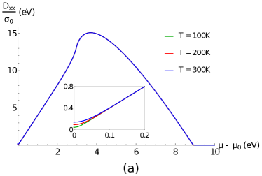
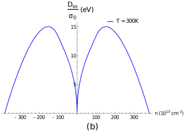
Figure 16: Drude weight results for SLG: (a) as a function of the Fermi level; (b) as a function of the carrier density. In (a), $\mu_{0}$ is the Fermi level at half filling.

We now move to the regular conductivity. The results are shown in Fig. 17. Here, and in what follows, we set $\Gamma=16$\mathrm{meV}$$ in agreement with Ref. (Ju2011, ). Once again, both methods —Eq. (154) for both real and imaginary parts or Eq. (154) for the real part along with Eq. (162) for the imaginary part— yield the same results and $\sigma_{xx}^{reg}=\sigma_{yy}^{reg},\ \sigma_{xy}^{reg}=0$. The fact that we obtain an isotropic (total) conductivity is an expected result from group theory since the system has hexagonal symmetry (Nowick1995, ). Analyzing Fig. 17(a), we interpret the peak at $\hbar\omega=2t\simeq 6$\mathrm{eV}$$ as electronic transitions from the van Hove singularity of the valence band to the van Hove singularity of the conduction band, as depicted by the red arrows in Fig. 18(a). These transitions are enhanced because there is a peak in the number of electrons that can occupy the initial and final energy states. Regarding Fig. 17(b), we also infer that transitions with $\hbar\omega<2\mu$ are forbidden, which has been observed experimentally (Li2008, ). The explanation is sketched in Fig. 18(b). When we increase the Fermi level up to $\mu>\mu_{0}$, states with $E<\mu$ become occupied. Therefore, transitions for those states are blocked due to the Pauli exclusion principle. Since we have particle-hole symmetry, we conclude that we can only have transitions when $\hbar\omega>2\mu$. The increase of the temperature is verified to smooth out this behavior (see Fig. 17(b)).

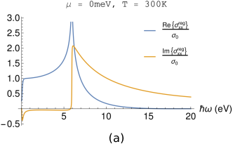
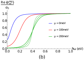
Figure 17: (a) and (b) show results for the regular conductivity in SLG. In (b), the dotted line corresponds to $T=100$\mathrm{K}$$, the dashed line to $T=200$\mathrm{K}$$ and the solid lines to $T=300$\mathrm{K}$$.

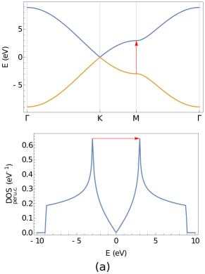
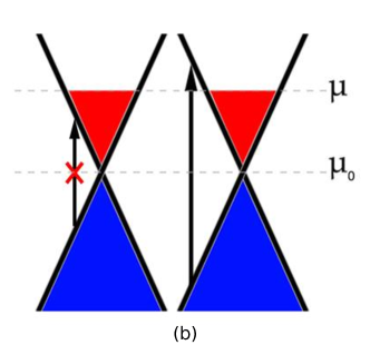
Figure 18: Picture of interband transitions in SLG. In (a), the spectrum and the DOS are plotted, showing the dominant transition that occurs between the van Hove singularities. In (b), the Pauli exclusion principle is depicted for the low-energy regime, where the Dirac cone picture is valid.

IV.1.3 Results for twisted bilayer graphene

A summary of the Drude weight results for tBLG is provided in Fig. 19. We stress that only the 2^nd method was verified to work well for these computations. This happens because we are working with an effective Hamiltonian, as discussed before. Similarly to what we have seen for the SLG, we observe symmetric results for electron or hole doping; this reflects the apparent symmetry in the valence and conduction bands mentioned in section III.3.2. By looking at Fig. 19(a), along with Fig. 14(a), we conclude that the Drude weight curve changes drastically (compared to SLG or decoupled BLG) when we cross van Hove singularities. This tendency coincides with what was found in Ref. (Stauber2013, ) and the drops in the curves are attributed to the fact that the first derivatives of the energy go to zero when we cross van Hove singularities. The effect of increasing the temperature is, as usual, the smoothing of this behavior.

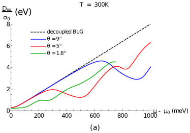
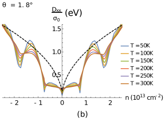
Figure 19: Drude weight results for tBLG ($2^{\text{nd}}$ method): (a) as a function of the Fermi level, for different twist angles; (b) as a function of the carrier density, for different temperatures. The outcomes were isotropic. In (b), the black dashed line is for decoupled BLG at $T=300$\mathrm{K}$$. The results for decoupled BLG (tBLG model with $t_{\perp}=0$) were verified to match the results for SLG multiplied by 2.

In Fig. 20(a), we show recent experimental results of the DC optical conductivity in the tBLG, obtained in Ref. (Cao2016, ). We observe the expected symmetry for doping with electrons and holes. Moreover, since for $\omega=0$ the conductivity is dominated by the Drude contribution, we may compare the experimental results with the theoretical calculations from Fig. 19(b). We note the need of including the disorder broadening $\Gamma$ in order to obtain a quantitative agreement with the experiment. In addition, we see that the experimental drop in the conductivity, at $|n|\sim 7.5\times 10^{12}${\mathrm{cm}}^{-2}$$, is in agreement with what our model predicts. These insulating states are interpreted as the gaps occurring at the $\Gamma_{m}$ point in the electronic spectrum (Fig. 20(b)). However, we immediately verify that the insulating behavior is much more pronounced in the experimental results. In the work done in Ref. (Cao2016, ), the authors estimated a band gap of $50-60$\mathrm{meV}$$, which is much larger than what we observe in the electronic spectrum. This effect might be due to the electron-electron interactions not considered in the model. Finally, we also note the disagreement between the experimental results and the theory near the Dirac point (which corresponds to $n=0$), in particular the fact that the conductivity is not very sensitive to $T$ below some value $T_{max}$ (see Fig. 20(a)). This is an expected feature observed in graphene and the explanation is that it occurs due to inhomogeneities in the system (extrinsic disorder, ripples, etc…), which make the Dirac point inaccessible (Morozov2008, ).

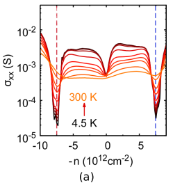
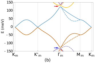
Figure 20: tBLG with $\theta=1.8^{\circ}$: (a) experimental results for the DC optical conductivity (source: Ref. (Cao2016, )); (b) electronic band structure.

In Figs. 21 and 22, we show representative results which allow us to analyze the regular conductivity in tBLG systems. All conductivity results obtained were isotropic. Just like in the SLG, this feature is expected from group theory since the tBLG also has an hexagonal symmetry (moiré pattern). Before discussing the results, we give a word about the numerical implementation of the real part (the imaginary part is straightforwardly computed from the real part by using the regularized KK relation). In contrast with the other calculations, where we only need to consider bands with $|E|\lesssim 1$\mathrm{eV}$$ (which are well described by the model), in this case we see that, for a given $\mu$ and for a given $\omega$, all bands with energy respecting $|E-\mu|\lesssim\hbar\omega$ contribute. Therefore, depending on the Fermi level $\mu$ and, most importantly, on the energy $\hbar\omega$ of the interband transition that we want to capture, we may need to consider higher energy bands that are not well described by the model. Still, this does not constitute a big concern because these bands lead to the well established constant value $2\sigma_{0}$, typical of the Dirac cone approximation.

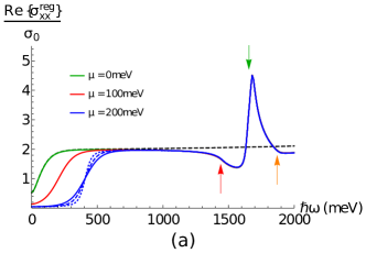
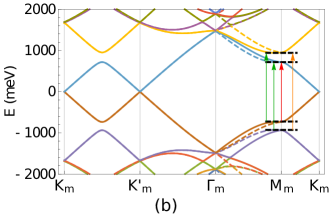
Figure 21: tBLG with $\theta=9^{\circ}$: (a) real part of the regular conductivity; (b) electronic spectrum. In (a), the dotted blue line corresponds to $T=100$\mathrm{K}$$, the dashed blue line to $T=200$\mathrm{K}$$ and the solid lines to $T=300$\mathrm{K}$$; the black dashed line is for decoupled tBLG (or SLG multiplied by 2) at $T=300$\mathrm{K}$$ and $\mu=0$.

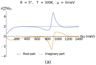
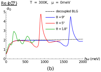
Figure 22: Regular conductivity results for tBLG at $\mu=0$: (a) real and imaginary parts for $\theta=5^{\circ}$; (b) real part for different $\theta$. In both (a) and (b), all dashed lines are for decoupled BLG or SLG multiplied by 2.

Looking at Fig. 21(a), we first notice the already discussed dependency on both the Fermi level and temperature. In addition, we observe a low-energy peak (marked with a green arrow), which we interpret as the dominant transitions shown in Fig. 21(b). Notice that there are other transitions (red and orange arrows) which we would also expect to be dominant, since they connect different van Hove singularities; however, these transitions are optically inactive, in agreement with what was found in Refs. (Tabert2013, ; Moon2013, ). This optical selection rule occurs due to a symmetry in the effective Hamiltonian which makes the matrix elements from Eq. (154) null for bands with symmetric energies at the $\text{M}_{m}$ points (Moon2013, ). From Fig. 22(a), we highlight the fact that the results obtained for the decoupled tBLG —tBLG with a null interlayer hopping parameter, $t_{\perp}=0$— match perfectly the results for SLG multiplied by 2. Although this was trivially expected, it was only achieved when we used the second method for computing the imaginary part of the regular conductivity; therefore, this served as a benchmark test for the validity of the computational methods. Moreover, we remark that we now have a region with a big deep on $\text{Im}\{\sigma^{reg}(\omega)\}$ occurring at lower frequencies, which will be an important feature in the next section. Regarding Fig. 22(b), we emphasize that, for small angles, we start to lose the “signature” behavior of the curves because of the presence of multiple low-energy van Hove singularities.

IV.2 Spectrum of surface plasmon-polaritons

IV.2.1 Dispersion relation — transverse magnetic modes

For this derivation, we will closely follow Ref. (Goncalves2016, ). We consider a system consisting of a single graphene sheet clad between two semi-infinite dielectric media, characterized by the real dielectric constants (relative permittivities) $\varepsilon_{1}^{r}$ and $\varepsilon_{2}^{r}$, as depicted in Fig. 23. We stress that, although the tBLG is not truly a 2D surface, its thickness is still negligible and we can view it as a monolayer for these purposes .

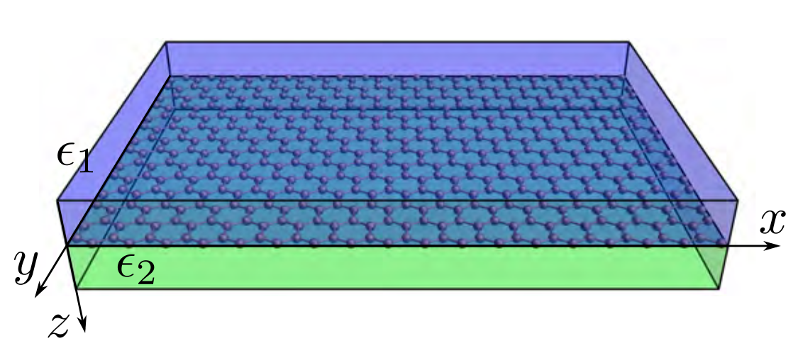
Figure 23: Illustration of a single graphene sheet sandwiched between two semi-infinite insulators with relative permittivities $\epsilon_{i}\equiv\varepsilon_{i}^{r}$ (in our notation). Medium 1 occupies the $z<0$ half-space and medium 2 the $z>0$; the graphene sheet is located at the $z=0$ plane. Source: Ref. (Goncalves2016, ).

Let us assume a solution of Maxwell’s equations in the form of a transverse magnetic (TM) wave. We use the following ansatz for the electric and magnetic fields in the medium $j=1,2$:

$$\bm{E}_{j}=(E_{j,x}\bm{\hat{x}}+E_{j,z}\bm{\hat{z}})e^{iqx}e^{-\kappa_{j}|z|},\quad\bm{B}_{j}=B_{j,y}e^{iqx}e^{-\kappa_{j}|z|}\bm{\hat{y}}.$$ (164)

This ansatz describes an electromagnetic wave (TM mode) which is confined to the neighborhood of the graphene sheet (with damping parameter $\kappa_{j}$ such that $\text{Re}\{\kappa_{j}\}>0$) and propagates along the $x$ direction. Due to translational invariance symmetry, the linear momentum along the propagation direction must be conserved, enabling us to write $q\equiv q_{1}=q_{2}$, where $q_{1/2}$ is the momentum of the electromagnetic wave propagating in medium $1/2$. Moreover, we note that we are just writing the spatial components of the fields; the time dependency, in what follows, is assumed to be of the typical harmonic form, i.e., $e^{-i\omega t}$.

We now make use of Maxwell’s equations. For each one of the media, Faraday’s law of induction and Ampère’s law read, respectively,

$$\bm{\nabla}\times\bm{E}_{j}=-\frac{\partial\bm{B}_{j}}{\partial t},$$ (165)

$$\bm{\nabla}\times\bm{H}_{j}=\bm{J}_{j}^{f}+\frac{\partial\bm{D}_{j}}{\partial t}.$$ (166)

Considering isotropic linear dielectric media, we can write the electric displacement as $\bm{D}_{j}=\varepsilon_{0}\varepsilon_{j}^{r}\bm{E}_{j}$, where $\varepsilon_{0}$ is the vacuum permittivity. Assuming isotropic linear magnetic media with unitary relative permeability, we may also write the magnetic field strength as $\bm{H}_{j}=\frac{\bm{B}_{j}}{\mu_{0}}$, where $\mu_{0}$ is the vacuum permeability. Finally, if the free current density is zero, $\bm{J}_{j}^{f}=\bm{0}$, we rewrite Ampère’s law as

$$\bm{\nabla}\times\bm{B}_{j}=\frac{\varepsilon_{j}^{r}}{c^{2}}\frac{\partial\bm{E}_{j}}{\partial t},$$ (167)

where $c=1/\sqrt{\mu_{0}\varepsilon_{0}}$ is the speed of light in vacuum. Introducing the fields given by Eq. (164) into Eqs. (165) and (167), we obtain the following useful relations:

$$-\text{sgn}(z)\kappa_{j}E_{j,x}-iqE_{j,z}=i\omega B_{j,y},$$ (168)

$$\text{sgn}(z)\kappa_{j}B_{j,y}=-i\omega\frac{\varepsilon_{j}^{r}}{c^{2}}E_{j,x},$$ (169)

$$iqB_{j,y}=-i\omega\frac{\varepsilon_{j}^{r}}{c^{2}}E_{j,z}.$$ (170)

From these, we can deduce

$$E_{j,x}=i\text{sgn}(z)\frac{\kappa_{j}c^{2}}{\omega\varepsilon_{j}^{r}}B_{j,y},$$ (171)

$$E_{j,z}=-\frac{qc^{2}}{\omega\varepsilon_{j}^{r}}B_{j,y},$$ (172)

$$\kappa_{j}^{2}=q^{2}-\frac{\omega^{2}\varepsilon_{j}^{r}}{c^{2}}.$$ (173)

Within the linear response regime, the boundary conditions linking the electromagnetic fields at $z=0$ read as

$$E_{1,x}(x,z=0)=E_{2,x}(x,z=0),$$ (174)

$$B_{1,y}(x,z=0)-B_{2,y}(x,z=0)=\mu_{0}J_{x}(x)=\mu_{0}\sigma_{xx}E_{2,x}(x,z=0),$$ (175)

which assure the continuity of the tangential component of the electric field across the interface and relate the discontinuity of the tangential component of the magnetic field to the surface current density. We emphasize that the conductivity of graphene is taken into account in the boundary conditions only. For unstrained graphene (and for the systems in focus), the conductivity is isotropic and frequency-dependent and so we write $\sigma(\omega)\equiv\sigma_{xx}=\sigma_{yy}$. From Eqs. (174) and (171), we get

$$B_{1,y}=-\frac{\kappa_{2}}{\kappa_{1}}\frac{\varepsilon_{1}^{r}}{\varepsilon_{2}^{r}}B_{2,y},$$ (176)

which we insert into Eq. (175) to obtain

$$\frac{\varepsilon_{1}^{r}}{\kappa_{1}(q,\omega)}+\frac{\varepsilon_{2}^{r}}{\kappa_{2}(q,\omega)}+i\frac{\sigma(\omega)}{\omega\varepsilon_{0}}=0.$$ (177)

This last equation describes the dispersion relation, $\omega(q)$, of TM SPPs. Notice that this is an implicit equation, so it needs to be solved numerically. Nonetheless, we can see that it can only have solutions when $\text{Im}\left\{\sigma(\omega)\right\}>0$.

IV.2.2 Results for single layer graphene

In Fig. 24, we present our results for the total conductivity (Drude plus regular terms) in SLG, as a function of the frequency, $f=\omega/(2\pi)$, across the spectral region where we are interested to study the spectrum of graphene SPPs —from the THz up to the mid-infrared. We recall that we have set $\Gamma=16$\mathrm{meV}$$; moreover, in the following results, we will always be considering room temperature, $T=300$\mathrm{K}$$. We also stress that we avoided exceeding frequencies of $30$\mathrm{THz}$$ because of the surface polar phonons that arise from the $\text{SiO}_{2}$ —the typical substrate used as medium 2—, according to Ref. (EduardoDias_tese, ) (Fig. 25).

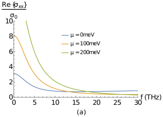
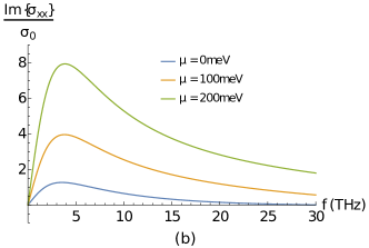
Figure 24: Total conductivity in SLG: (a) real part; (b) imaginary part.

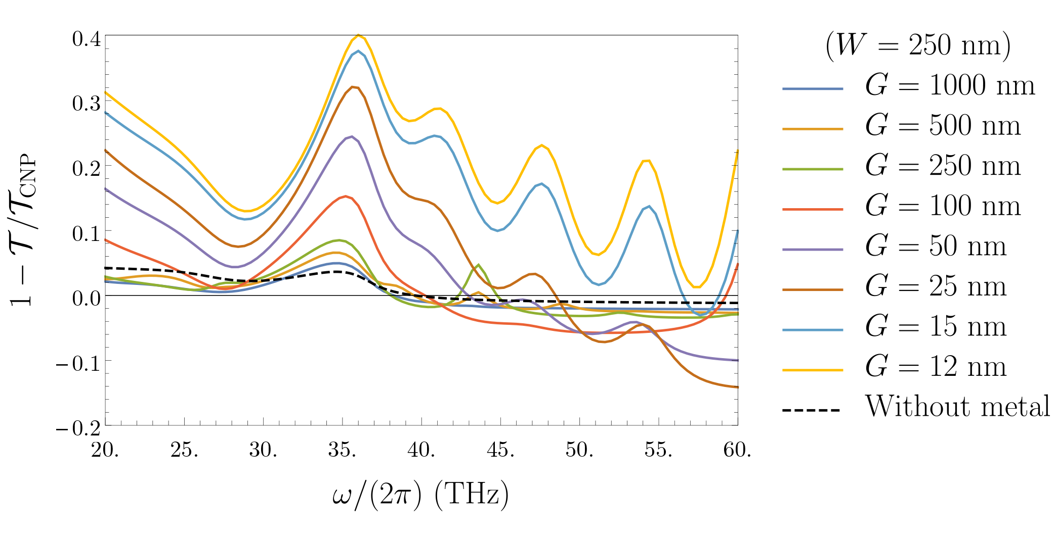
Figure 25: Evidence of surface optical phonons arising from the $\text{SiO}_{2}$ substrate. In this plot, the quantity in focus is the optical transmittance, $\mathcal{T}$, with $\mathcal{T}_{\text{CNP}}$ being the optical transmittance at the charge neutrality point. This quantity was obtained within a theoretical calculation, which takes into account the full dielectric function of the $\text{SiO}_{2}$. The parameters $W$ and $G$ correspond to $a$ and $d-a$, respectively, in the scheme of Fig. 15. The peak that starts at $f\sim 30\,\text{THz}$ was interpreted as a contribution from the $\text{SiO}_{2}$ optical phonons. Source: Ref. (EduardoDias_tese, ).

Given the total conductivity at a given Fermi level, we can obtain the dispersion curve by solving Eq. (177) numerically. Notice that, if we consider only the Drude contribution with $\Gamma=0$, we have a pure imaginary conductivity and we can solve this equation with real $q$. If not, we have to consider a complex-valued wave vector, whose imaginary part characterizes the attenuation of the SPPs (BludovFerreiraPeresEtAl2013, ; Goncalves2016, ). In Fig. 26, we present the spectrum of SPPs in SLG for $\mu=450$\mathrm{meV}$$, which we obtained by taking into account the total conductivity. This curve is in agreement with the results obtained in Ref. (Goncalves2016, ), namely with Fig. 4.2, where the authors considered only the Drude contribution (which is the dominant term in this case) with no absorption ($\Gamma=0$), and Fig. 4.3, where they verified that the consideration of absorption ($\Gamma\neq 0$) only affects the spectrum in the region of low wave vectors. Analyzing the spectrum, we see that the dispersion curve lies to the right of the light line, which indicates, as we have mentioned before, that we cannot excite graphene SPPs simply by directly shining electromagnetic radiation . It is now clear why we need to use a setup with a periodic grid, like the one described in section IV (see Fig. 15).

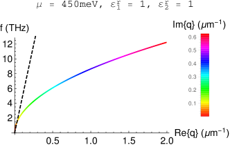
Figure 26: Dispersion relation of TM SPPs in SLG. The dashed line corresponds to the light dispersion, $\omega=cq$, where $c$ is the speed of the light in the medium (in this case, air).

At last, we can fix a wave vector —physically, if we take the light line as roughly vertical, this corresponds to fixing a gap in the periodic grid— and study the dependency of the dispersion curves on the Fermi level (or the carrier density). The results are shown in Fig. 27. We stress that we do not obtain $f(n=0)=0$ in Fig. 27(a) because of the finite temperature.

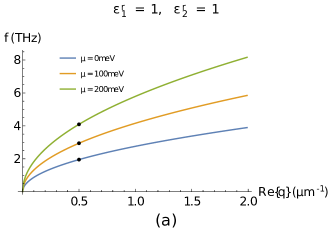
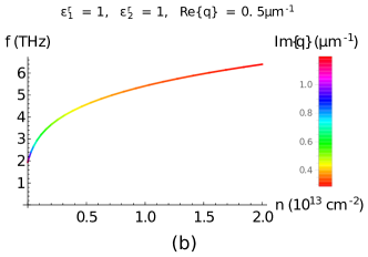
Figure 27: Spectrum of TM SPPs in SLG: dependency on the Fermi level/carrier density. Panel (a) schematically shows the procedure used to obtain panel (b).

IV.2.3 Results for twisted bilayer graphene

For the tBLG, we repeat the previous analysis, namely the last 2 plots from Fig. 27, for two different twist angles. We start with $\theta=9^{\circ}$ (Fig. 28). For this angle, we see that the signature of the curves do not differ a lot from those of the SLG. This happens due to two main reasons:

• Within this range of frequency, $f\lesssim 30$\mathrm{THz}$\Leftrightarrow\hbar\omega\lesssim 124$\mathrm{meV}$$, the regular conductivity is basically twice the value obtained for the SLG (see Fig. 21(a)). Moreover, for $\mu\lesssim 250$\mathrm{meV}$$, the Drude weight is also twice the value obtained for the SLG (see Fig. 19(a)). Therefore, we do not capture any hybridization effect and we just recover the total conductivity of a decoupled BLG.

• As we can see in Fig. 14(b), the curves $n(\mu)$ for $\theta=9^{\circ}$ and for decoupled BLG are also very close within the range in focus, $\mu\lesssim 250$\mathrm{meV}$\Leftrightarrow n\lesssim 1\times 10^{13}${\mathrm{cm}}^{-2}$$.

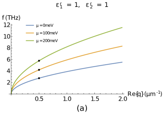
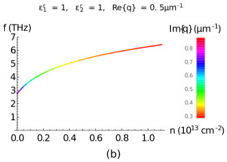
Figure 28: Spectrum of TM SPPs in tBLG with $\theta=9^{\circ}$: dependency on the Fermi level/carrier density. The black dots in (a) mark the fixed parameter in (b).

We move on to the angle $\theta=1.8^{\circ}$ (Fig. 29). In this case, not only the total conductivity is different but also the relation $n(\mu)$ changes drastically. This leads to the plot of Fig. 29(b), which we highlight since it is totally different from all the results obtained before. As an immediate application, we can think of using these results as an alternative method for determining the twist angle. Nevertheless, a more extensive study on the behavior of these curves with the variation of $\theta$ remains to be done, in order to investigate more promising applications.

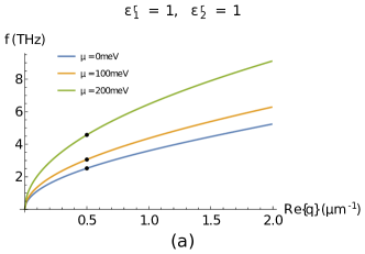
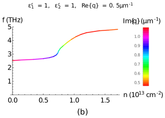
Figure 29: Spectrum of TM SPPs in tBLG with $\theta=1.8^{\circ}$: dependency on the Fermi level/carrier density. The black dots in (a) mark the fixed parameter in (b).

As future work, we shall also consider a frequency range for which the big deep on $\text{Im}\left\{\sigma^{reg}(\omega)\right\}$ of tBLG (seen in Fig. 22(a) for $\theta=5^{\circ}$) plays a role. By varying the twist angle, this deep can be brought to arbitrary low frequencies. However, at some point, the contribution from the Drude conductivity will dominate. In between, we can find a regime for which the total conductivity has a negative imaginary part. In this case, Eq. (177) has no solutions and therefore we cannot sustain TM modes. Instead, we will have transverse electric modes, which were not addressed in this chapter. With this, we can explore the use of tBLG as a polarizer for waveguide modes.

V Conclusions

In this chapter we provided a pedagogical introduction to the electronic and optical properties of twisted bilayer graphene. We started, in section II, with a brief description of the tight-binding models for single layer graphene and perfectly aligned Bernal-stacked bilayer graphene. We explicitly showed how the electronic bands of single layer graphene fold when larger than the minimal unit cells are considered, and how to obtain the corresponding Hamiltonian directly in reciprocal space. From this, we moved to the description of twisted bilayer graphene in section III. We saw how the interference between the periodicities of the two misaligned layers leads to the emergence of a moiré pattern. We also saw how the properties of the electrons moving in this moiré pattern can be described starting from a tight-binding Hamiltonian, expressing the electronic wave function in terms of Bloch-waves of each layer and considering generalized umklapp processes. With this machinery, we studied how the interlayer coupling leads to a twist-angle-dependent renormalization of the Fermi velocity, in the weak coupling limit. We also showed how to describe the electronic spectrum beyond the weak coupling limit, by including a greater number of generalized umklapp processes. With the spectrum reconstruction established, we computed the profiles of the density of states and the carrier density. We observed that the electronic spectrum is strongly modified by varying the twist angle, namely by bringing van Hove singularities to lower energies and thus making them easily accessible via electrostatic doping. Having established the electronic spectrum of the twisted bilayer graphene, we addressed its optical properties in section IV. Within the linear response theory, we presented a derivation of general tight-binding-based expressions to compute both the regular and the Drude contributions to the homogeneous optical conductivity, which are suitable for low-energy effective models. Applying these expressions to the twisted bilayer graphene, we observed that the conductivity profiles can be drastically modified by varying the twist angle. We then used these results to study the dispersion relation of surface plasmon-polaritons in twisted bilayer graphene.

We expect that the research in twisted bilayer graphene will continue to reveal new and interesting physics, with potential applications, and that these findings will further guide research into other kinds of van der Waals structures.

At the time of writing, electron-electron interactions in twisted bilayer graphene were an underdeveloped topic. This suddenly changed after the experimental findings of correlated insulator behavior Cao2018a and superconductivity Cao2018 in doped magic-angle twisted bilayer graphene.

- (1) A. K. Geim. Graphene: status and prospects. Science, 324(5934):1530–1534, 2009.
- (2) S. Z. Butler, S. M. Hollen, L. Cao, Y. Cui, J. A. Gupta, H. R. Gutiérrez, T. F. Heinz, S. S. Hong, J. Huang, A. F. Ismach, E. Jonhston-Halperin, M. Kuno, V. V. Plashnitsa, R. D. Robinson, R. S. Ruoff, S. Salahuddin, J. San, L. Shi, M. G. Spencer, M. Terrones, W. Windl, J. E. Goldberger. Progress, challenges, and opportunities in two-dimensional materials beyond graphene. ACS nano, 7(4):2898–2926, 2013.
- (3) S. Das, J. A. Robinson, M. Dubey, H. Terrones, M. Terrones. Beyond graphene: progress in novel two-dimensional materials and van der Waals solids. Annu. Rev. Mater. Res., 45:1–27, 2015.
- (4) K. S. Novoselov, A. H. C. Neto. Two-dimensional crystals-based heterostructures: materials with tailored properties. Phys. Scr., T146:014006, 2012.
- (5) K. S. Novoselov, A. Mishchenko, A. Carvalho, A. H. C. Neto. 2D materials and van der Waals heterostructures. Science, 353(6298):aac9439, 2016.
- (6) J. M. B. Lopes dos Santos, N. M. R. Peres, A. H. C. Neto. Continuum model of the twisted graphene bilayer. Phys. Rev. B, 86(15):155449, 2012.
- (7) I. Brihuega, P. Mallet, H. González-Herrero, G. Trambly de Laissardière, M. M. Ugeda, L. Magaud, J.M. Gómez-Rodríguez, F. Ynduráin, J.-Y. Veuillen. Unravelling the intrinsic and robust nature of van Hove singularities in twisted bilayer graphene. Phys. Rev. Lett., 109(19):196802, 2012.
- (8) S. Latil, V. Meunier, L. Henrard. Massless fermions in multilayer graphitic systems with misoriented layers: ab initio calculations and experimental fingerprints. Phys. Rev. B, 76(20):201402, 2007.
- (9) E. S. Morell, J. D. Correa, P. Vargas, M. Pacheco, Z. Barticevic. Flat bands in slightly twisted bilayer graphene: tight-binding calculations. Phys. Rev. B, 82(12):121407, 2010.
- (10) G. T. de Laissardière, D. Mayou, L. Magaud. Numerical studies of confined states in rotated bilayer of graphene. Phys. Rev., 86(12):125413, 2012.
- (11) J. M. B. Lopes dos Santos, N. M. R. Peres, A. H. C. Neto. Graphene bilayer with a twist: electronic structure. Phys. Rev. Lett., 99(25):256802, 2007.
- (12) R. Bistritzer, A. H. MacDonald. Moiré bands in twisted double-layer graphene. PNAS, 108(30):12233–12237, 2011.
- (13) R. de Gail, M. O. Goerbig, F. Guinea, G. Montambaux, A. H. C. Neto. Topologically protected zero modes in twisted bilayer graphene. Phys. Rev. B, 84(4):045436, 2011.
- (14) Mikito Koshino. Interlayer interaction in general incommensurate atomic layers. New Journal of Physics, 17(1):015014, 2015.
- (15) D. Weckbecker, S. Shallcross, M. Fleischmann, N. Ray, S. Sharma, O. Pankratov. Low-energy theory for the graphene twist bilayer. Phys. Rev. B, 93(3):035452, 2016.
- (16) A. K. Geim, A. H. MacDonald. Graphene: exploring carbon flatland. Phys. Today, 60(8):35–41, 2007.
- (17) A. H. C.Neto, F. Guinea, N. M. R. Peres, K. S. Novoselov, A. K. Geim. The electronic properties of graphene. Rev. Mod. Phys., 81(1):109, 2009.
- (18) S. Reich, J. Maultzsch, C. Thomsen. Tight-binding description of graphene. Phys. Rev. B, 66(3):035412, 2002.
- (19) C. Bena, G. Montambaux. Remarks on the tight-binding model of graphene. New J. Phys., 11(9):095003, 2009.
- (20) Indranil Paul, Gabriel Kotliar. Thermal transport for many-body tight-binding models. Phys. Rev. B, 67:115131, Mar 2003.
- (21) D. K. Efetov, P. Kim. Controlling electron-phonon interactions in graphene at ultrahigh carrier densities. Phys. Rev. Lett., 105(25):256805, 2010.
- (22) A. Das, S. Pisana, B. Chakraborty, S. Piscanec, S. K. Saha, U. V. Waghmare, K. S. Novoselov, H. R. Krishnamurthy, A. K. Geim, A. C. Ferrari, A. K. Sood. Monitoring dopants by Raman scattering in an electrochemically top-gated graphene transistor. Nature nanotechnology, 3(4):210–215, 2008.
- (23) K. F. Mak, C. H. Lui, J. Shan, T. F. Heinz. Observation of an electric-field-induced band gap in bilayer graphene by infrared spectroscopy. Phys. Rev. Lett., 102(25):256405, 2009.
- (24) M. Fleck, AN. M. Oleś, L. Hedin. Magnetic phases near the van Hove singularity in s-and d-band Hubbard models. Phys. Rev. B, 56(6):3159, 1997.
- (25) J. González. Kohn-Luttinger superconductivity in graphene. Phys. Rev. B, 78(20):205431, 2008.
- (26) R. Nandkishore, L. S. Levitov, A. V. Chubukov. Chiral superconductivity from repulsive interactions in doped graphene. Nature Physics, 8(2):158–163, 2012.
- (27) G. Li, A. Luican, J. M. B. Lopes dos Santos, A. H. Castro Neto, A. Reina, J. Kong, E. Y. Andrei. Observation of van Hove singularities in twisted graphene layers. Nature Physics, 6(2):109–113, 2010.
- (28) A. V. Rozhkov, A. O. Sboychakov, A. I. Rakhmanov, F. Nori. Electronic properties of graphene-based bilayer systems. Physics Reports, 648:1–104, 2016.
- (29) Pablo San-Jose, A. Gutiérrez-Rubio, Mauricio Sturla, Francisco Guinea. Spontaneous strains and gap in graphene on boron nitride. Phys. Rev. B, 90:075428, Aug 2014.
- (30) J. C. Slater, G. F. Koster. Simplified LCAO method for the periodic potential problem. Phys. Rev., 94(6):1498–1524, 1954.
- (31) A. Kretinin, G. L. Yu, R. Jalil, Y. Cao, F. Withers, A. Mishchenko, M. I. Katsnelson, K. S. Novoselov, A. K. Geim, F. Guinea. Quantum capacitance measurements of electron-hole asymmetry and next-nearest-neighbor hopping in graphene. Phys. Rev. B, 88(16):165427, 2013.
- (32) Y. Wang, Z. Ni, L. Liu, Y. Liu, C. Cong, T. Yu, X. Wang, D. Shen, Z. Shen. Stacking dependent optical conductivity of bilayer graphene. ACS nano, 4(7):4074–4080, 2010.
- (33) X. Zou, J. Shang, J. Leaw, Z. Luo, L. Luo, C. La o vorakiat, L. Cheng, S. A. Cheong, H. Su, J.-X. Zhu, Y. Liu, K. P. Loh, A. H. C. Neto, T. Yuand E. E. M. Chia. Terahertz conductivity of twisted bilayer graphene. Phys. Rev. Lett., 110(6):067401, 2013.
- (34) Y. Cao, J. Y. Luo, V. Fatemi, S. Fang, J. D. Sanchez-Yamagishi, K. Watanabe, T. Taniguchi, E. Kaxiras, P. Jarillo-Herrero. Superlattice-induced insulating states and valley-protected orbits in twisted bilayer graphene. Phys. Rev. Lett., 117(11):116804, 2016.
- (35) C.J. Tabert, E.J. Nicol. Optical conductivity of twisted bilayer graphene. Phys. Rev. B, 87(12):121402, 2013.
- (36) P. Moon, M. Koshino. Optical absorption in twisted bilayer graphene. Phys. Rev. B, 87(20):205404, 2013.
- (37) Tobias Stauber, Pablo San-Jose, Luis Brey. Optical conductivity, Drude weight and plasmons in twisted graphene bilayers. New J. Phys., 15(11):113050, 2013.
- (38) L. Ju, B. Geng, J. Horng, C. Girit, M. Martin, Z. Hao, H. A. Bechtel, X. Liang, A. Zettl, Y. R. Shen, F. Wang. Graphene plasmonics for tunable terahertz metamaterials. Nature nanotechnology, 6(10):630–634, 2011.
- (39) M. Jablan, H. Buljan, M. Soljačić. Plasmonics in graphene at infra-red frequencies. Phys. Rev. B, 80(24):245435, 2009.
- (40) F. H. L. Koppens, D. E. Chand, F. J. G. de Abajo. Graphene plasmonics: a platform for strong light–matter interactions. Nano Lett., 11(8):3370–3377, 2011.
- (41) X. Luo, T. Qiu, W. Lu, Z. Ni. Plasmons in graphene: recent progress and applications. Materials Science & Engineering, R: Reports, 74(11):351–376, 2013.
- (42) A. Vakil, N. Engheta. Transformation optics using graphene. Science, 332(6035):1291–1294, 2011.
- (43) Z. Fang, Y. Wang, Z. Liu, A. Schlather, P. M. Ajayan, F. H. L. Koppens, P. Nordlander, N. J. Halas. Plasmon-induced doping of graphene. ACS nano, 6(11):10222–10228, 2012.
- (44) Z. Fei, A. S. Rodin, G. O. Andreev, W. Bao, A. S. McLeod, M. Wagner, L. M. Zhang, Z. Zhao, M. Thiemens ang G. Dominguez, M. M. Fogler, A. H. C. Neto, C. N. Lau, F. Keilmann, D. N. Basov. Gate-tuning of graphene plasmons revealed by infrared nano-imaging. Nature, 487(7405):82–85, 2012.
- (45) J. Chen, M. Badioli, P. Alonso-González, S. Thongrattanasiri, F. Huth, J. Osmond, M. Spasenović, A. Centeno, A. Pesquera, P. Godignon, A. Zurutuza, N. Camara, J. G. de Abajo, R. Hillenbrand, F. Koppens. Optical nano-imaging of gate-tuneable graphene plasmons. Nature, 487(7405):77–81, 2012.
- (46) A. N. Grigorenko, M. Polini, K. S. Novoselov. Graphene plasmonics. Nat. Photonics, 6(11):749–758, 2012.
- (47) P. A. D. Gonçalves, N. M. R. Peres. An introduction to graphene plasmonics. World Scientific Publishing Co. Pte. Ltd., 2016.
- (48) D. J. Passos, G. B. Ventura, J. M. Viana Parente Lopes, J. M. B. Lopes dos Santos, N. M. R. Peres. Nonlinear optical responses of crystalline systems: results from a velocity gauge analysis. Phys. Rev. B, 97(23):235446, 2018.
- (49) N. A. Doughty. Lagrangian interaction. Addison-Wesley, 1990.
- (50) N. W. Ashcroft, N. D. Mermin. Solid state physics. Harcourt College Publishers, 1976.
- (51) C. Kittel. Introduction to solid state physics. John Wiley & Sons, 1966.
- (52) T. Stauber, N. M. R. Peres, A. K. Geim. The optical conductivity of graphene in the visible region of the spectrum. Phys. Rev. B, 78(8):085432, 2008.
- (53) Arthur S. Nowick. Crystal properties via group theory. Cambridge University Press, 1995.
- (54) Z. Q. Li, E. A. Henriksen, Z. Jiang, Z. Hao, M. C. Martin, P. Kim, H. L. Stormer, D. N. Basov. Dirac charge dynamics in graphene by infrared spectroscopy. Nature Physics, 4(7):532–535, 2008.
- (55) S. V. Morozov, K. S. Novoselov, M. I. Katsnelson, F. Schedin, D. C. Elias, J. A. Jaszczak, A. K. Geim. Giant intrinsic carrier mobilities in graphene and its bilayer. Phys. Rev. Lett., 100(1):016602, 2008.
- (56) A. K. Geim, K. S. Novoselov. The rise of graphene. Nat. Mater., 6(3):183–191, 2007.
- (57) Eduardo J. C. Dias. Plasmonic effects in unidimensional structures and graphene-based nanostructures. Praca magisterska, Universidade do Minho, Nov 2016.
- (58) Y. V. Bludov, A. Ferreira, N. M. R. Peres, M. I. Vasilevskiy. A primer on surface plasmon-polaritons in graphene. Int. J. Mod. Phys. B, 27(10):1341001, 2013.
- (59) Yuan Cao, Valla Fatemi, Ahmet Demir, Shiang Fang, Spencer L. Tomarken, Jason Y. Luo, Javier D. Sanchez-Yamagishi, Kenji Watanabe, Takashi Taniguchi, Efthimios Kaxiras, Ray C. Ashoori, Pablo Jarillo-Herrero. Correlated insulator behaviour at half-filling in magic-angle graphene superlattices. Nature, 556(7699):80–84, 2018.
- (60) Yuan Cao, Valla Fatemi, Shiang Fang, Kenji Watanabe, Takashi Taniguchi, Efthimios Kaxiras, Pablo Jarillo-Herrero. Unconventional superconductivity in magic-angle graphene superlattices.