Mass composition of cosmic rays above 0.1 EeV by the Yakutsk array data

Abstract

The paper presents the results of the longitudinal development of extensive air showers (X_max) of ultra-high energies and mass composition of cosmic rays. The measurements of X_max are based on data from observations of the Cherenkov radiation at the Yakutsk array for the period 1974-2014. The cascade curves of individual showers and the depth of maximum X_max were reconstructed over the energy range 10¹⁶-5.7$\cdot$10¹⁹ eV. It is shown that the displacement rate of the parameter dX_max / dE in the atmosphere is nonlinear and depends on the energy. Such a feature indicates a change in mass composition, which is confirmed by fluctuations of X_max in this energy region. The composition of cosmic rays was determined by interpolation using the QGSJetII-04 model.

I Introduction

Knowledge of the mass composition (MC) of cosmic rays (CR) in the energy range above 0.1 EeV is very important for astrophysics. It is assumed that a transition from galactic to extra-galactic CR (Berezhko et al., 2012) is within the energy range of 0.1-1 EeV, also irregularities like ”dip-bump” at energies above 5 EeV (Berezinsky et al., 2006), and cutoff of the spectrum of CR associated with the GZK effect at energies $\sim$50 EeV (Greisen, 1966; Zatsepin and Kuzmin, 1966).

One of the crucial techniques in the study of the characteristics of CR by Extensive Air Shower (EAS) method is Vavilov-Cherenkov radiation (Zrelov, 1968; Jelley, 1958) detection, which is produced by shower particles in the visible wavelength. The total flux of Cherenkov light allows determining the energy of the primary particle and the lateral distribution at sea level provides information on the nature of the development of a shower in the atmosphere (Knurenko et al., 2001).

Longitudinal development of the shower in the atmosphere was reconstructed by the lateral distribution function (LDF) of Cherenkov light (Knurenko et al., 2001; Dyakonov et al., 1986) using the inverse problem method (Tikhonov and Arsenin, 1977). To estimate the mass composition, the depth of maximum of air shower development X_max was used, which is sensitive to the atomic mass of the primary particle.

At the Yakutsk array, in order to estimate air shower energy we used the energy balance method (Knurenko et al., 2006a). The method is based on the energy dissipated by EAS particles in the atmosphere, i.e. full flux of Cherenkov light. In individual showers, the energy was determined by the flux density of Cherenkov light at a distance R = 200 m from the shower axis - Q (200). According to calculations, the classification parameter Q (200) is proportional to the shower energy and have little shower-to-shower fluctuations.

The average depth of the air shower maximum X_max was used to derive CR MC within the hadronic interaction model QGSJetII-04 (Ostapchenko, 2011) according to (Hörandel, 2006).

The Yakutsk array consists of stations with scintillation and Cherenkov detectors to register elementary particles of different nature: hadrons, electrons and positrons, muons, and Cherenkov photons (Artamonov et al., 1994). Additionally, there are surface electric field and air shower radio emission observations (Knurenko et al., 2017). The array consists of 120 scintillation detectors located on an area of $\sim$13 km². Three muon stations and 72 channels for integrated and differential Cherenkov detectors are located at the center (Knurenko et al., 1998; Garipov et al., 2001; Ivanov et al., 2015; Egorov et al., 2018) (Fig. 1). The observation energy range of the array is from 10¹⁵ eV to 10²⁰ eV, which allows it to study both galactic and extra-galactic CR.

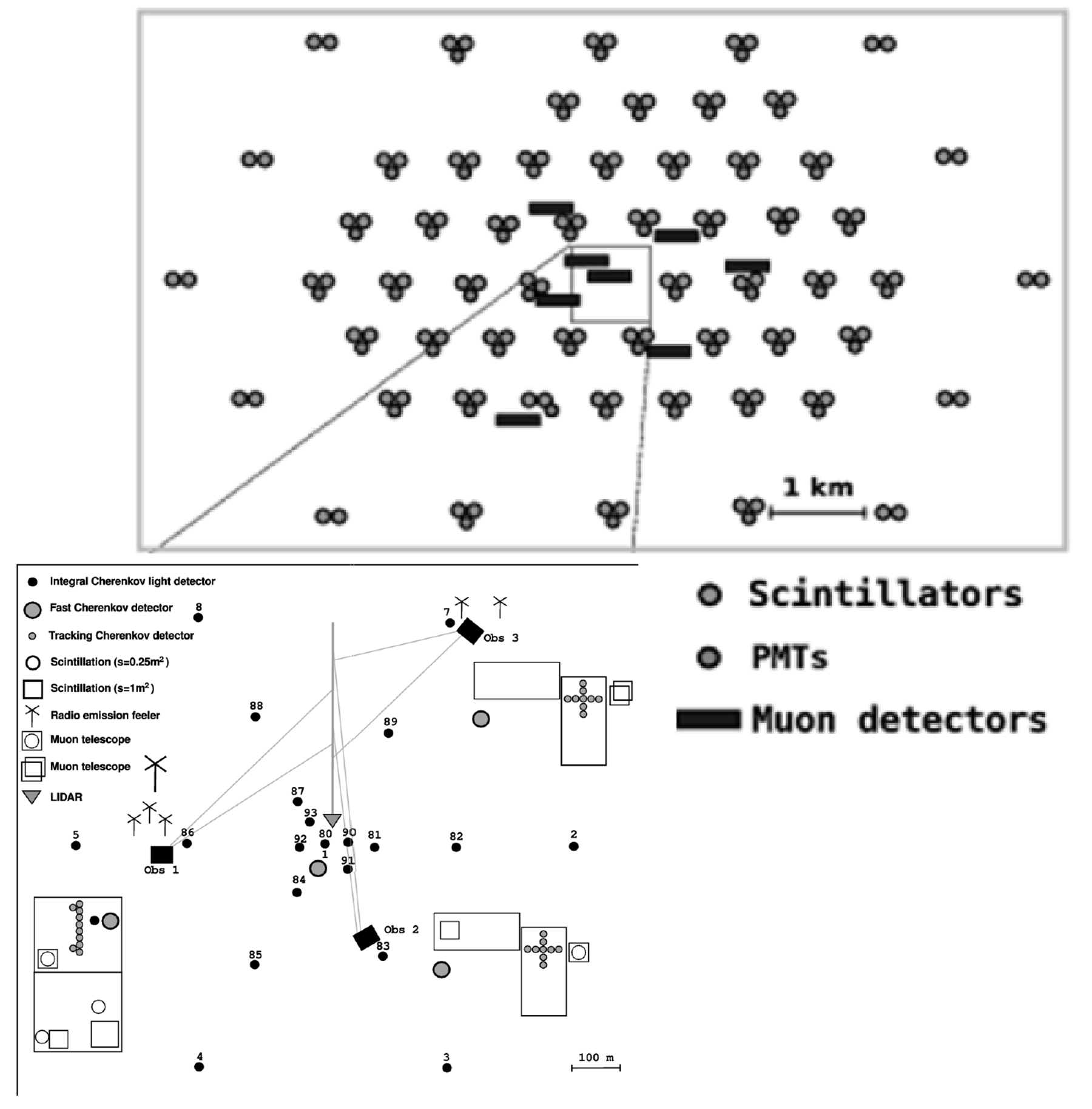
Figure 1: Arrangement of the observation stations at the Yakutsk array

Cherenkov measurements are conducted on clear and moon-less nights. The observation season starts in September and ends in April. The total observation time per season is 450-600 hours, which takes 6-10$\%$ of the annual array operation time. Since optical observations are very sensitive to such atmospheric characteristics as transparency and the aerosol component of the atmosphere (Dyakonov et al., 1999; Zuev, 1970), the atmosphere is monitored daily at the array (Dyakonov et al., 1991; Knurenko et al., 2006b; Knurenko and Petrov, 2014).

II Experimental data and analysis

II.1 Reconstruction of air shower parameters

The depth of maximum X_max is determined by the cascade curve of Cherenkov light, which is reconstructed from the experimental Cherenkov LDF (Fig. 2) (Knurenko et al., 2001). This algorithm is described in detail in (Knurenko et al., 2001; Dyakonov et al., 1986). The algorithm is based on the Fredholm equation of the first kind (1), which is solved by the adaptive method (Kochnev, 1985):

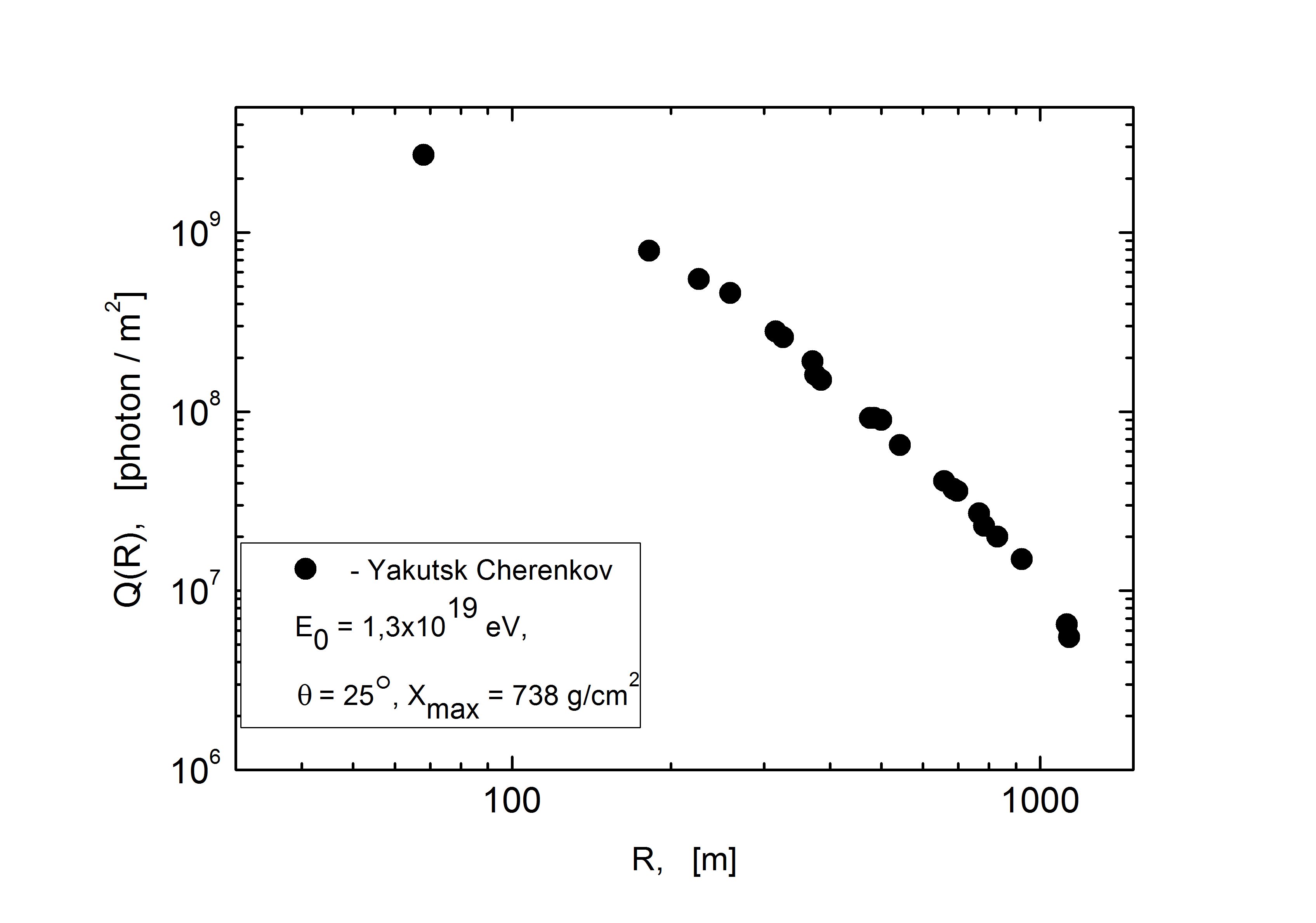
Figure 2: LDF of the Cherenkov light

$$Q_{exp}=\delta_{Q}+\int_{X_{1}}G(R,X/X_{2})\cdot N(E_{0},X)\cdot K(\lambda,X)dX$$ (1)

In equation (1), $G(R,X/X_{2})$ is the function that represents the lateral-angular distribution of electrons in the electron-photon cascade. In our case, the function $G(R,X/X_{2})$ takes into account the nonequilibrium spectrum of electrons (Belyaev et al., 1980; Dyakonov, 1982), i.e. depends on the age of the shower and is close to the data from Hillas (Hillas, 1982; Patterson and Hillas, 1983) and Giller (Giller et al., 2004). More recent work (Nerling et al., 2006; Smialkowski and Giller, 2018) confirms the correctness of the use of lateral-angular distribution that depends on the age of the shower, for X_max reconstruction by Cherenkov light of air showers. The use of different models of lateral-angular distribution from the ”equilibrium” approximation and, including calculations of the electron spectra depending on shower age, yielded 3-5$\%$ in the spread of the X_max estimation. N (E₀, X) is a cascade curve, $\delta$Q is the ”noise” level, depends on measurement uncertainty and data processing errors. The choice of lateral-angular distribution was made in (Knurenko, 2003). K ($\lambda$, X) is transmittance of the atmosphere that takes into account the transmission of Cherenkov light throughout the entire thickness of the atmosphere. The coefficient K ($\lambda$, X) was reconstructed by solving the inverse problem using the lateral distribution of Cherenkov light registered under different weather conditions by a photomultiplier with a maximum sensitivity at a wavelength of $\lambda$ = 430 nm (Dyakonov et al., 1999). Reconstructed dependence of Cherenkov light transmission coefficient for different weather conditions on the height is shown in Fig. 3. Approximation of these data is also given there.

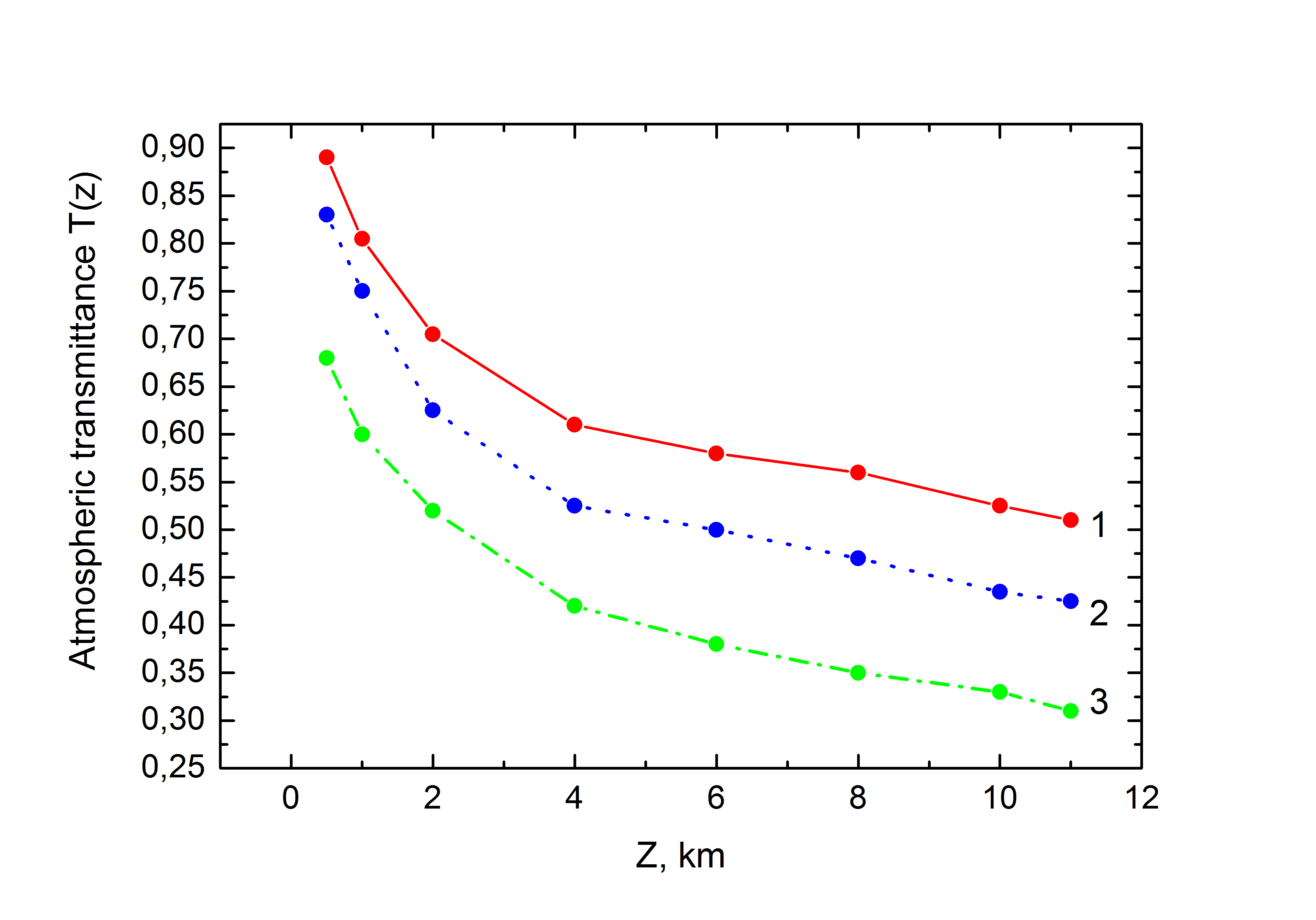
Figure 3: Vertical profile of atmospheric transmittance coefficient for different conditions: 1- 5 points; 2- four points; 3- three points (Dyakonov et al., 1999)

For the prompt estimation of atmospheric conditions during the registration of air showers in the optical wavelength at the Yakutsk array, a point system for estimation of the state of the atmosphere was developed. The estimation was tested by instrumental methods, including the rate of triggers for showers with energies of 10¹⁵-10¹⁶ eV (Dyakonov et al., 1991). The point system for classification of the atmosphere was proposed in the papers (Knurenko et al., 2006b; Guschin, 1988) based on lidar measurements of the spectral transparency P_λ and spectral atmospheric optical thickness $\delta_{\lambda}$. The correlation results for the three wavelengths are given in Table 1.

Table 1: Different values for P_λ and $\delta_{\lambda}$ in different scales of the atmosphere transparency.

Atmospheric transparency	Pλ=530	$\delta_{\lambda=530}$	Pλ=369	$\delta_{\lambda=369}$	Pλ=430
low (2 points)	0.60	0.180	0.35	0.260	0.48
decreased (3 points)	0.70	0.080	0.46	0.120	0.56
normal (3 - 4 points)	0.75	0.060	0.50	0.080	0.60
increased (4 points)	0.80	0.040	0.52	0.060	0.68
high (5 points)	0.85	0.020	0.56	0.030	0.72

X₁ and X₂ - upper and lower limits of the atmosphere for air shower development. The limits were used for reconstruction of the air shower cascade curve.

As seen from equation (1), the method takes into account the physics of air shower electron-photon component development and characteristics of the atmospheric conditions during registration of the Cherenkov radiation (Knurenko et al., 2006b; Knurenko and Petrov, 2014) at the Yakutsk array. Using this technique, average cascade curves were reconstructed (Fig. 4) for energies of $\sim$10¹⁸ and $\sim$10¹⁹ eV (Tikhonov and Arsenin, 1977) and compared with QGSJetII-04 simulations. As can be seen from Fig. 4, the experimental cascade curve is measured in a wide range of depths due to inclined showers. This circumstance was used to determine the absorption range of cascade particles beyond the maximum development of air showers (Glushkov et al., 1993). On the other hand, cascade curves can be used to test different models of the development of air shower in the atmosphere.

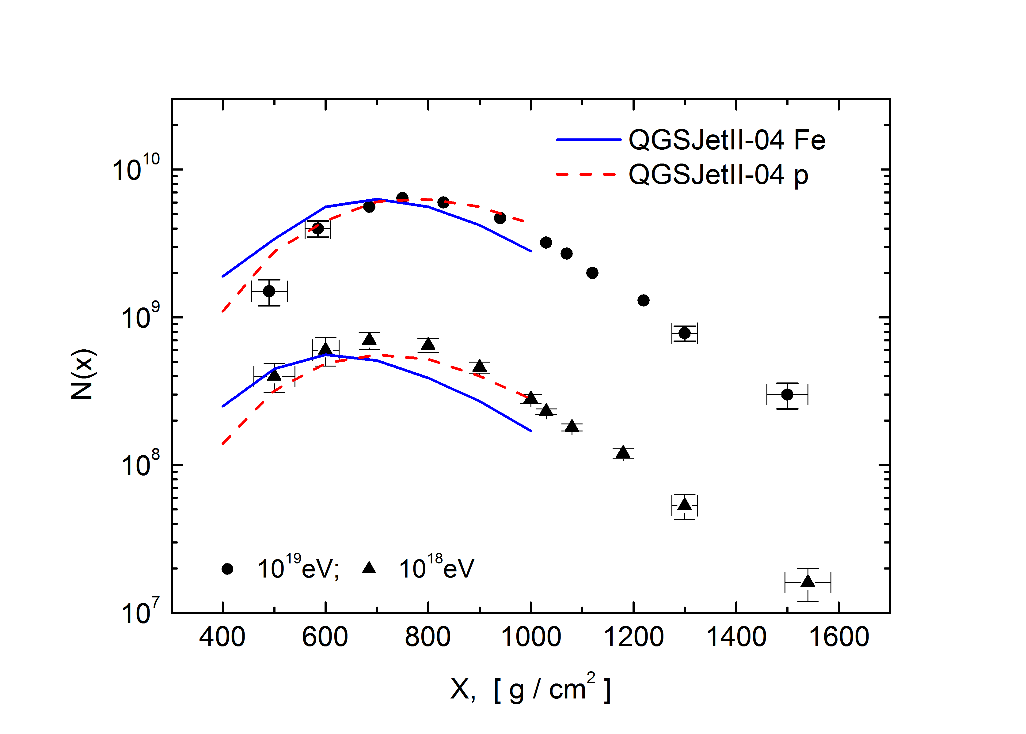
Figure 4: Average experimental cascade curves and calculations by QGSJETII-04 (Ostapchenko, 2011) for proton and iron

The energy at the Yakutsk array was determined by energy balance method of all air shower particles (Knurenko et al., 2006a). This suggests that the total energy of the shower takes into account the ionization losses of each of the components of air shower: electrons, muons, hadrons and neutrinos (see formula (2)).

$$E_{0}=E_{ei}+E_{el}+E_{\mu}+E_{hi}+E_{\mu i}+E_{\nu}$$ (2)

Their share of energy was determined empirically taking into account the experiment conducted at the Yakutsk array. For example, the ionization losses of the electronic component were determined by the total flux of Cherenkov light from air showers, according to formula (3):

$$E_{ei}=k(x,P_{\lambda})\cdot\Phi$$ (3)

where $\Phi$ is the total flux of Cherenkov light; k (x, P_λ) is the approximation coefficient (calculated value), takes into account the transparency of the real atmosphere, the nature of the longitudinal development of the shower (energy spectrum of secondary particles and its dependence on the age of the shower) and expressed through the depth of the maximum of air shower X_max, measured at the array (Knurenko et al., 2006a; Ivanov et al., 2015).

As can be seen from Fig. 5, the fraction of E_em is 85-90$\%$, fraction of the remaining components of the shower does not exceed 10$\%$, and their estimation is described in details in papers (Knurenko et al., 2006a; Ivanov et al., 2015).

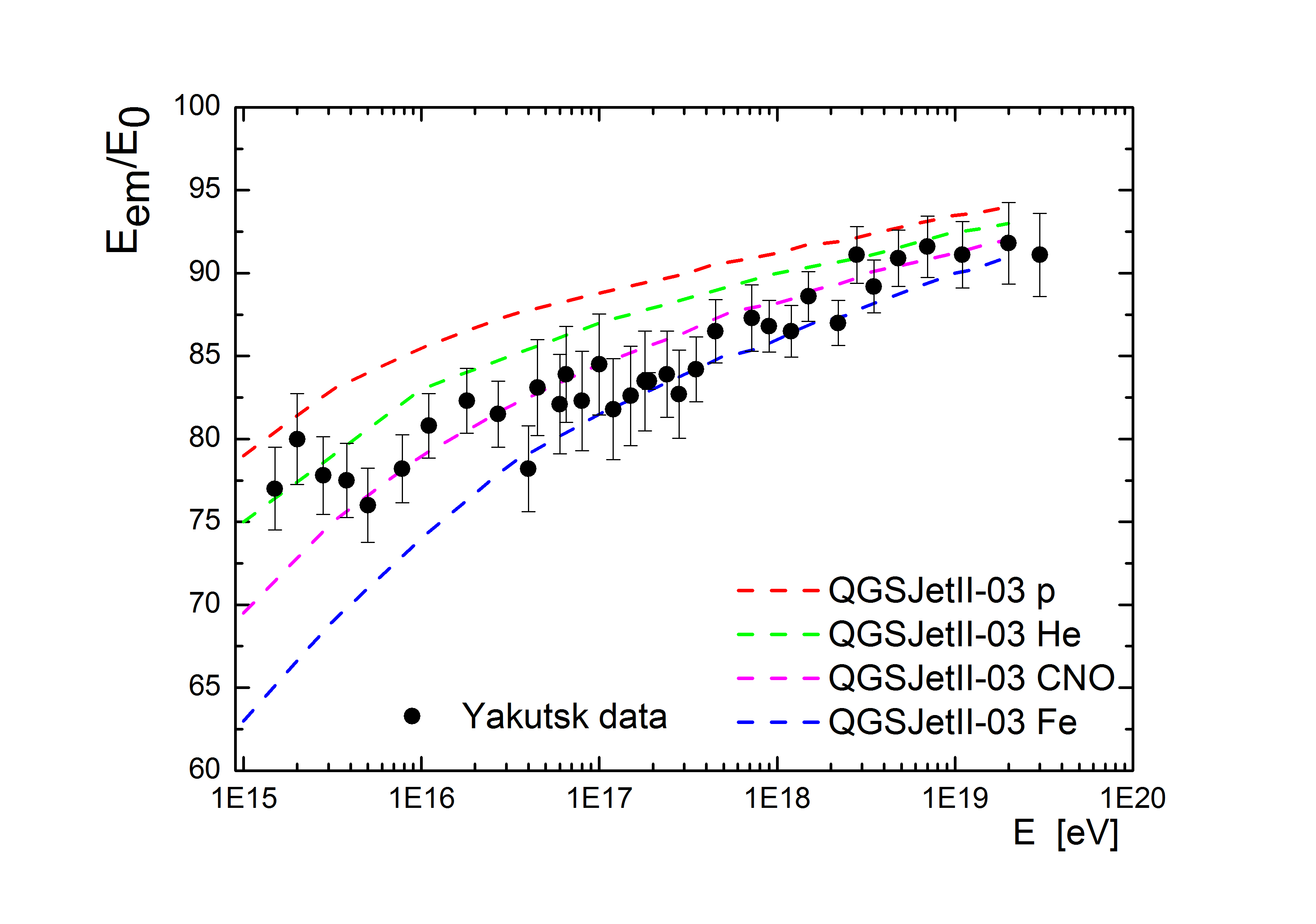
Figure 5: The fraction of energy transferred to the electromagnetic component according to the registration of Cherenkov light of air shower at the Yakutsk array and hadronic interactions model QGSJetII-03 for proton p, helium He, CNO nuclei and iron nucleus Fe

The experimental data of the Yakutsk array are in good agreement with the calculations by the QGSjetII-03 model in the case of a mixed composition of primary particles. This estimate may change if other models are used, including the QGSjetII-04 (Ostapchenko, 2011). This is stated in our work (Knurenko et al., 2005). In papers (Abbasi et al., 2018a; Barbosa et al., 2004), the calculations of E_em / E₀ were performed to estimate the energy of air showers registered at the HiRes and TA arrays. Based on the calculations and the experiment in Yakutsk, it can be said that with an accuracy of 10$\%$, there is agreement on the energy estimates in both arrays.

A test check of the reconstruction method was carried out using QGSjet-01 calculations of the Cherenkov light of air showers. The result of comparing the cascade curve calculated by the model for the energy of 10¹⁸ eV and reconstructed by the method described above showed a good agreement Knurenko et al. (2001).

II.2 Air shower reconstruction uncertainty

Measurement errors in our experiment are systematic and random (Knurenko et al., 2015). The main source of systematic uncertainty is the absolute calibration error due to the uncertainty of the transition from the amplitude of the signal at the output of the PMT to the number of Cherenkov light photons. It is determined by the coupling coefficient between the amplitudes of the signals from the reference light source and the plastic scintillator unit, which serves as a calibration light source. The relative error of this coefficient is $\delta_{Q_{cal}}$ = 21$\%$.

Random measurement errors are due to many factors. One of them is the instrumental error of response measurement itself, equal to $\delta_{Q_{app}}$ = 13$\%$. For the short (R $<$ 100 m) distances from the axis, a similar contribution is made by axis determination method, the absolute error of which for showers selected by the central part of the array is $\Delta$R = 10 m for the approximation of Q (R) by a piecewise-power function with value of n $\sigma_{loc}$ = n$\cdot\Delta$ (R / R_thresh.). Along with this, there are Q (R) distortions due to the shower processing procedure. These include the use of different test functions with different boundary conditions for the density of charged particles, the classification of showers according to different measured parameters, the threshold of the Cherenkov light detector. The study of these distorting factors shows that in this case measurement errors of Q (R) increase at small and large (R$>$ 800 m) distances from the shower axis. The influence of the detector threshold begins to affect from a distance of R$>$ 600 m, depending on the energy of the primary particle. It is expressed in the fact that due to the random nature of the detector triggering at the threshold level, zero readings are underestimated and the value of the Cherenkov light flux begins to be systematically overestimated. For E₀ = 2$\cdot$10¹⁸ eV, this overestimation is 5$\%$ and 20$\%$ at distances of 600 and 800 m, respectively, and this fact had to be taken into account when processing showers. For this reason, showers for the analysis were selected only by the central part of the array, where the symmetry condition of the location of observation stations relative to the air shower axis was met and all showers had approximately the same uncertainty for the reconstruction of the air shower characteristics.

Above mentioned uncertainties were taken into account for reconstruction of the cascade curve according to formula (4):

$$\sigma_{Q_{i}}^{2}=\left(0.04+n^{2}\cdot\left(\frac{\Delta R}{R}\right)^{2}\cdot Q^{2}_{i}\right)$$ (4)

Here $\Delta$R - is error of air shower axis determination error, 0.04 - constant associated with the absolute calibration of the light receivers and n - slope value of the power approximation of Cherenkov light LDF.

Uncertainty of the X_max reconstruction for individual showers was 15-55 g/cm² (Knurenko, 2003; Knurenko et al., 2001). Uncertainty of energy estimation at the Yakutsk array, taking into account the measurements uncertainties listed above is 23-26$\%$ (Knurenko et al., 2006a; Ivanov et al., 2009).

II.3 Depth of maximum development X_max

The analysis presented in this paper is based on the Yakutsk array 1974-2014 dataset. The showers selected for analysis are shown in Fig. 6, as the dependence of X_max on the classification parameter of air showers Q (200) - Cherenkov light flux density at the distance 200 m from the shower axis. The flux density of the Cherenkov light has little shower-to-shower fluctuations and weakly depends on zenith angle (Kalmykov, 1967; Knurenko, 2003), therefore Q(200) was used as the classification parameter for air shower selection. The energy of the shower is derived from Q (200) parameter by formula (5) (Knurenko et al., 2006a):

$$E_{0}=(1.78\pm 0.44)\cdot 10^{17}\cdot\left(\frac{Q(200)}{10^{17}}\right)^{1.01\pm 0.04}$$ (5)

In the distribution of air showers given in Fig.6, there are events with X_max $\geq$ 800 g / cm², i.e. with the low depth of maximum development compared to iron or even proton induced air showers. These showers can be used to search for neutral particles such as $\gamma$-rays and neutrinos (Knurenko and Petrov, 2018).

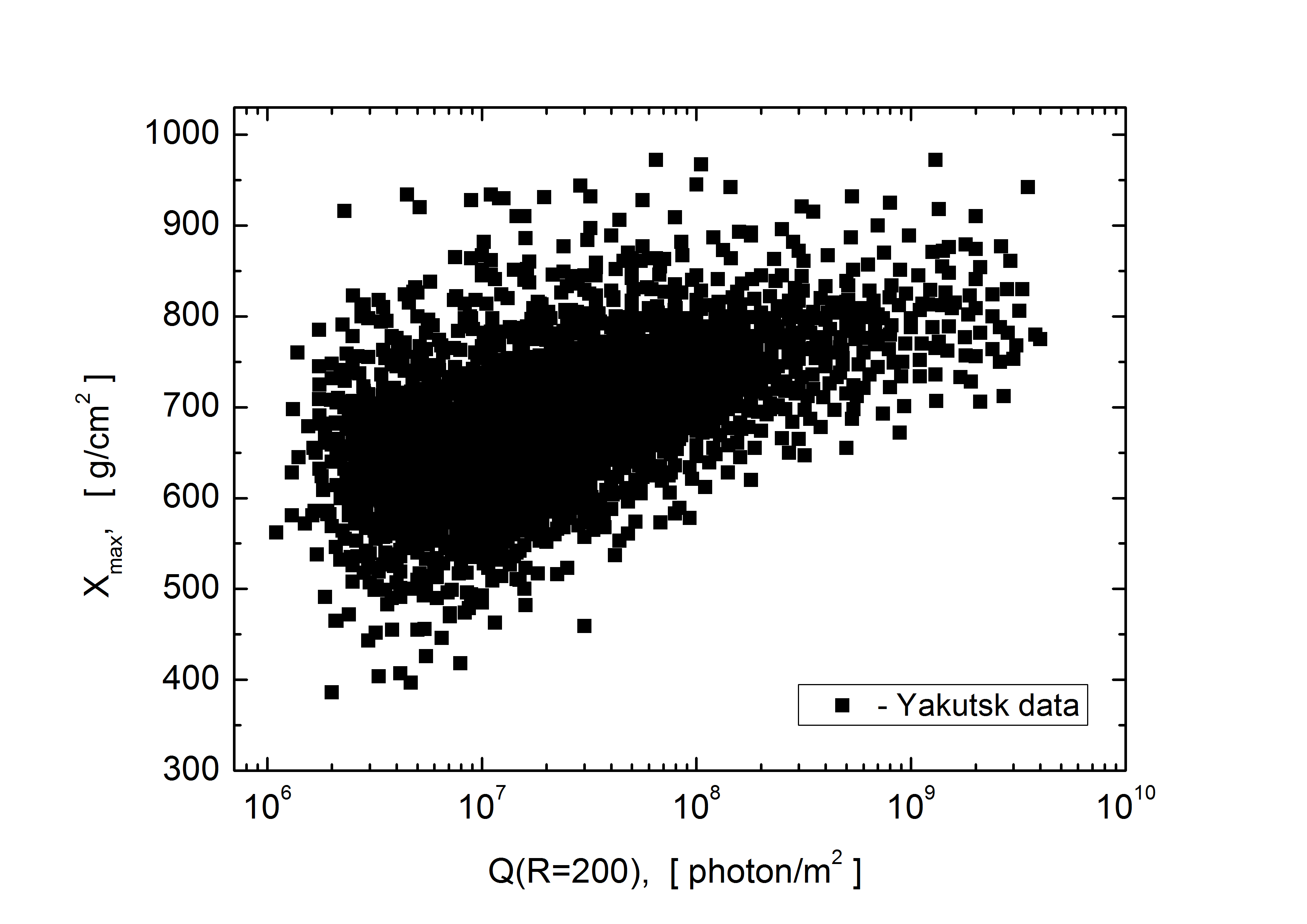
Figure 6: Dependence of X_max from classification parameter Q (200) - EAS Cherenkov light flux density at a distance of 200 m from the shower axis.

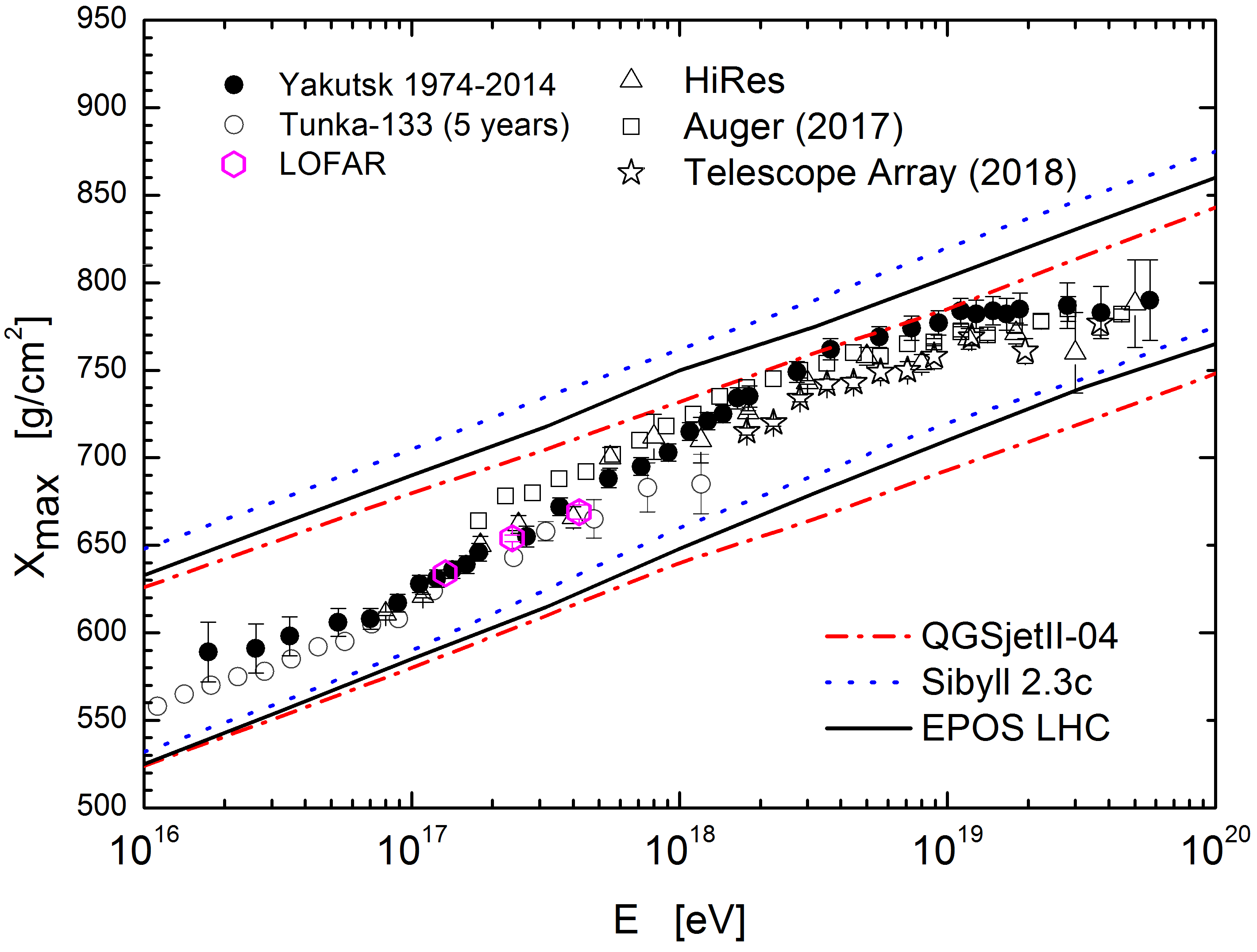
a)

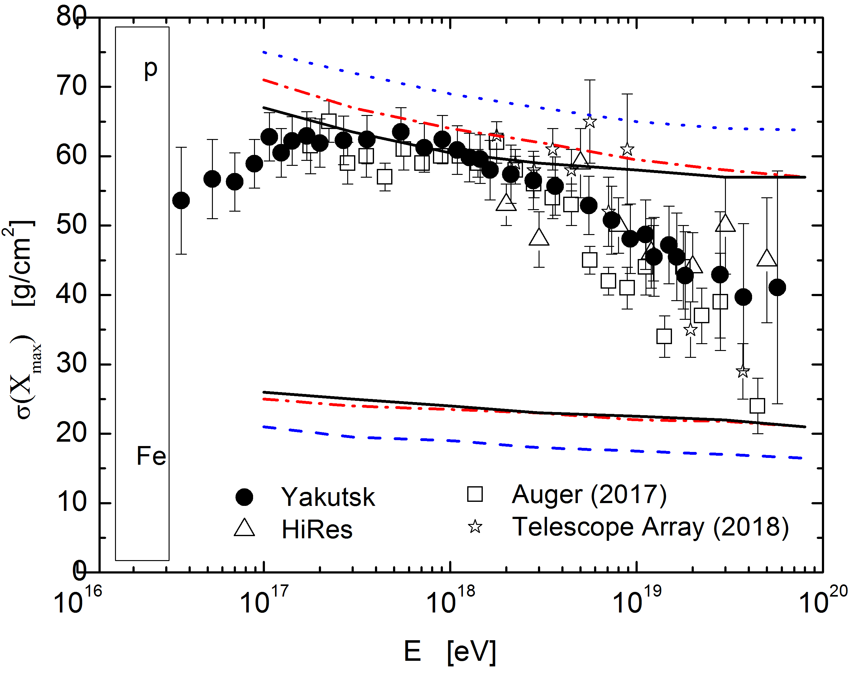
b)

Figure 7: The mean (a) and the standard deviation (b) of the measured X_max distributions as a function of energy obtained from Cherenkov light data in 1974-2014 at the Yakutsk array. Comparison with other experiments: Auger (Bellido et al., 2018), TA (Abbasi et al., 2018b), HiRes (Abbasi et al., 2010; Ulrich and Cazon, 2012), Tunka (Prosin et al., 2016), LOFAR (Buitink et al., 2016) and simulations for proton and iron primaries by different models QGSJetII-04 (Ostapchenko, 2011), Sibyll 2.3c (Riehn et al., 2015), EPOS LHC (Pierog et al., 2015).

The averaged data of the Yakutsk array together with the data of the Auger (Bellido et al., 2018), TA (Abbasi et al., 2018b), HiRes (Abbasi et al., 2010; Ulrich and Cazon, 2012), Tunka (Prosin et al., 2016), LOFAR (Buitink et al., 2016) arrays are shown in Fig. 7 (a) and comparison with different hadronic interaction models QGSJetII-04 (Ostapchenko, 2011), Sibyll 2.3c (Riehn et al., 2015), EPOS LHC (Pierog et al., 2015). The data within the experimental errors are in good agreement with each other, although they were obtained at different experiments and by different methods. The data of the Yakutsk array covers almost four orders of magnitude in energy. Statistics allows with sufficient accuracy to identify the shift of X_max with increasing energy and to estimate the elongation rate (ER) at different energy ranges. According to our data, the ER is:

1. E = 10¹⁶-10¹⁷ [eV]; E.R. = 48$\pm$6 [ g/cm² ]

2. E = 10¹⁷-10¹⁸ [eV]; E.R. = 78$\pm$5 [ g/cm² ]

3. E = 10¹⁸-10¹⁹ [eV]; E.R. = 63$\pm$6 [ g/cm² ]

4. E = 10¹⁹-10²⁰ [eV]; E.R. = 50$\pm$7 [ g/cm² ]

The data $\langle X_{max}\rangle$, $\sigma$(X_max) and other characteristics are given in Tables 2, 3.

In Fig. 7 (b) X_max fluctuations are presented. These fluctuations were obtained taking into account detectors effect according to the method given below. The accuracy of the X_max reconstruction was estimated from the simulation of cascade curve reconstruction process by full Monte Carlo method, given the known values of the instrumental uncertainty Q(E₀, R, X₀) and parameters of the average cascade curve. It was assumed that the measurement uncertainty Q(E₀, R, X₀) are distributed according to the normal law (Dyakonov et al., 1981, 1983). As follows from (Dyakonov et al., 1981, 1983) $\sigma(X_{max})_{app}$ depends not only on measurements uncertainty Q(E₀, R, X₀), but also on coordinates of the shower axis relative to the array center (X₀, Y₀) and the number of stations n participating in the registration of the Cherenkov EAS light. So the average instrumental error at an energy of 10¹⁸ eV is equal to $<\sigma(X_{max})_{app}>$ = 38 g / cm², and its dependence on energy can be expressed as:

$$\langle\sigma(X_{max})_{app}\rangle=(38.5\pm 5)-(10\pm 3)\lg\frac{E_{0}}{10^{18}}$$ (6)

Then physical fluctuations $\sigma(X_{max})$ were found as the difference of measured fluctuations and instrumental fluctuations:

$$\sigma^{2}(X_{max})=\sigma^{2}(X_{max})_{meas}-\sigma^{2}(X_{max})_{app}$$ (7)

The data was divided by energy with a step of 1.5, and the value $\sigma$(X_max) was found for each interval. The figure contains data obtained at the Yakutsk array and data of Auger, TA and HiRes. The figure also shows calculations using modern models of hadron interactions for the primary proton and the iron nucleus.

From Fig. 7 (b) one can see there is a maximum of X_max fluctuations dependency on energy in the range 2$\cdot$10¹⁷-2$\cdot$10¹⁸ eV. In this range, the value of $\sigma$(X_max) is 57-63 g/cm², which according to model calculations corresponds to the mixed composition of cosmic rays with a high content of p + He and heavier nuclei. However, the composition consisting of a mix of 50% proton p and 50${\%}$ iron nuclei Fe cannot be excluded. A decrease in fluctuations above the energy of 5$\cdot$10¹⁸ eV indicates a heavier composition.

II.4 Mass composition

Knowing the depth of the shower maximum X_max (Fig. 7, a) and average X_max for the proton and the iron nucleus from QGSJetII-04 simulations, the value of $\langle lnA\rangle$ can be determined by interpolation using formula (8) (Berezhko et al., 2012; Hörandel, 2006):

$$\langle lnA\rangle=\frac{X^{exp}_{max}-X^{p}_{max}}{X^{Fe}_{max}-X^{p}_{max}}\cdot lnA_{Fe}$$ (8)

where X${}^{exp}_{max}$ is the depth of maximum determined from the experiment, $lnA_{Fe}$ is the natural logarithm of the iron atomic mass.

The mean logarithmic mass values are presented for different energies in Fig. 8. The results are compared with data of Tunka (Prosin et al., 2016), LOFAR Buitink et al. (2016), TA (Abbasi et al., 2019) and Auger (Bellido et al., 2018), derived using the hadronic interaction model QGSJetII-04. There is also the Yakutsk array data for 1994-2010 (Knurenko and Sabourov, 2011)]. This result was obtained for limited data selection with QGSJETII model, which explains discrepancy with the data presented in current paper As can be seen from the figure, there are irregularities of the value of $\langle lnA\rangle$, due to MC change. For example, in the energy region of 10¹⁶-10¹⁷ eV, the composition is heavier than in the energy region of 10¹⁷-10¹⁸ eV, where composition mostly consists of protons p and helium He nuclei. Starting from $\sim$10¹⁹ eV, the composition becomes heavier, i.e. the fraction of such nuclei as CNO and Fe iron nuclei increases.

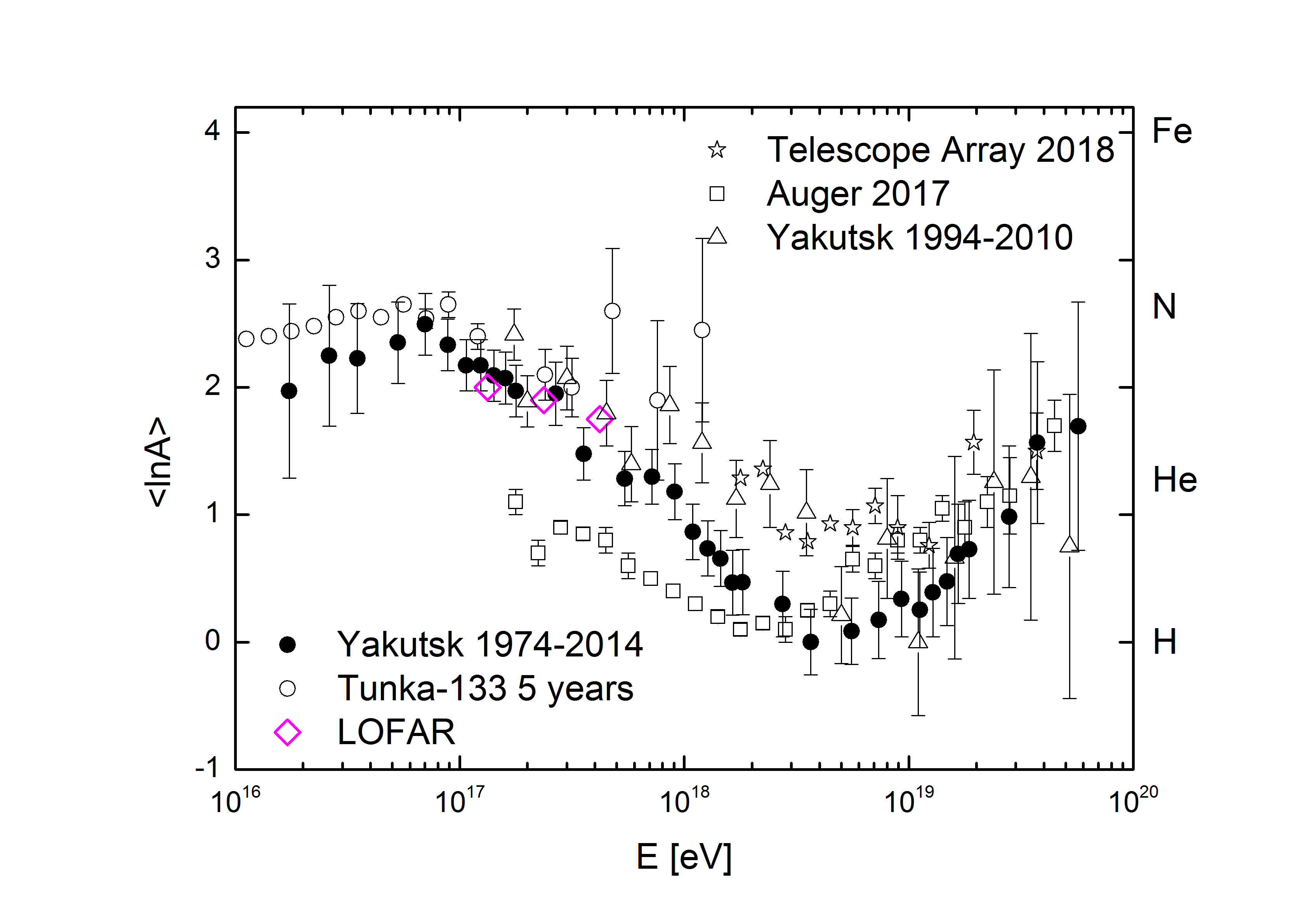
Figure 8: Average atomic mass $\langle lnA\rangle$ derived from the average depth of the shower maximum with QGSJetII-04 (Ostapchenko, 2011). Comparison with Yakutsk (1994-2010)(Knurenko and Sabourov, 2011), Tunka (Prosin et al., 2016), LOFAR (Buitink et al., 2016), TA (Abbasi et al., 2019) and Auger (Bellido et al., 2018) data.

Table 2: $\left\langle X_{max}\right\rangle$ , $\sigma$( X_max ) and $\left\langle lnA\right\rangle$ observed in 1974-2014 at the Yakutsk array.10¹⁶ - 10¹⁸ eV

E0, eV	N, events	Xmax, g/cm2	$\sigma$(Xmax), g/cm2	$\langle lnA\rangle$	$\langle lnA\rangle$ stat. error
1.74E+16	-	589$\pm$17	-	1.97	0.68
2.62E+16	-	591$\pm$14	-	2.25	0.55
3.50E+16	24	598$\pm$11	53.6$\pm$7.7	2.23	0.43
5.31E+16	50	606$\pm$8	56.7$\pm$5.7	2.35	0.32
7.01E+16	88	608$\pm$6	56.3$\pm$4.2	2.50	0.24
8.85E+16	139	617$\pm$5	58.9$\pm$3.5	2.34	0.20
1.07E+17	158	628$\pm$5	62.8$\pm$3.5	2.17	0.20
1.24E+17	146	631$\pm$5	60.5$\pm$3.5	2.17	0.20
1.42E+17	155	636$\pm$5	62.2$\pm$3.5	2.09	0.20
1.60E+17	158	639$\pm$5	62.9$\pm$3.5	2.07	0.20
1.78E+17	153	646$\pm$5	61.9$\pm$3.5	1.97	0.20
2.68E+17	155	655$\pm$5	62.3$\pm$3.5	1.95	0.25
3.57E+17	156	672$\pm$5	62.4$\pm$3.5	1.48	0.21
5.43E+17	161	688$\pm$5	63.5$\pm$3.5	1.28	0.21
7.18E+17	150	695$\pm$5	61.2$\pm$3.5	1.30	0.22
9.06E+17	155	703$\pm$5	62.4$\pm$3.5	1.18	0.22

Table 3: $\left\langle X_{max}\right\rangle$ , $\sigma$( X_max ) and $\left\langle lnA\right\rangle$ observed in 1974-2014 at the Yakutsk array. 10¹⁸ $\cdot$5.7$\cdot$10¹⁹ eV

E0, eV	N, events	Xmax, g/cm2	$\sigma$(Xmax), g/cm2	$\langle lnA\rangle$	$\langle lnA\rangle$ stat. error
1.09E+18	148	715$\pm$5	60.9$\pm$3.5	0.87	0.22
1.27E+18	143	721$\pm$5	59.8$\pm$3.5	0.73	0.22
1.45E+18	142	725$\pm$5	59.6$\pm$3.5	0.66	0.22
1.64E+18	93	734$\pm$6	58.0$\pm$4.3	0.47	0.25
1.82E+18	92	735$\pm$6	57.4$\pm$4.2	0.47	0.26
2.74E+18	89	749$\pm$6	56.5$\pm$4.2	0.30	0.26
3.66E+18	86	762$\pm$6	55.7$\pm$4.2	0	0.26
5.56E+18	78	769$\pm$6	52.9$\pm$4.2	0.09	0.26
7.35E+18	53	774$\pm$7	50.8$\pm$4.9	0.17	0.30
9.27E+18	47	777$\pm$7	48.1$\pm$5.0	0.34	0.30
1.12E+19	48	784$\pm$7	48.7$\pm$5.0	0.25	0.30
1.28E+19	32	782$\pm$8	45.5$\pm$5.7	0.39	0.35
1.48E+19	35	784$\pm$8	47.2$\pm$5.6	0.48	0.35
1.66E+19	26	782$\pm$9	45.5$\pm$6.3	0.69	0.39
1.86E+19	23	785$\pm$9	42.8$\pm$6.3	0.73	0.39
2.80E+19	11	787$\pm$13	42.9$\pm$9.1	0.99	0.56
3.74E+19	7	783$\pm$15	39.7$\pm$10.6	1.57	0,64
5.69E+19	3	790$\pm$23	41.1$\pm$16.8	1.69	0.97

III Conclusion

The Yakutsk array is operating continuously for more than 45 years, detecting electrons, muons, Cherenkov light, and radio emission. At the same time, more than 5$\cdot$10⁶ EAS events were recorded in the energy region above 10¹⁵ eV. Using a large dataset of air showers with energies of 10¹⁶-5.7$\cdot$10¹⁹ eV, registered for the period 1974-2014, the longitudinal development of showers was reconstructed and the $X_{max}$ dependence was found. The results showed that elongation rate per decade of energy has nonlinear advancement and takes the values 48$\pm$6, 78$\pm$5, 63$\pm$6, 50$\pm$7 g / cm² for energy ranges, 10¹⁶-10¹⁷, 10¹⁷-10¹⁸, 10¹⁸-10¹⁹, 10¹⁹-10²⁰ eV. As can be seen (Fig. 7), there are kinks at the energies $\sim$10¹⁷ eV and $\sim$5$\cdot$10¹⁸ eV, i.e. on the ”second knee” area and the beginning of irregularities in the spectrum like ”dip-bump”. As shown by the data of the Yakutsk array (Fig. 8), this is due to a change in the cosmic ray mass composition. At low energies up to 10¹⁷ eV, there are noticeably more nuclei with an atomic mass of 4-56, at energies of 10¹⁷-10¹⁸ eV the proportion of protons increases and reaches a maximum, accounting for 60-80$\%$. In the region of energy greater than 10¹⁹ eV, CR predominantly consist of helium nuclei He, CNO, and heavier elements.

References

References

- Berezhko et al. (2012) E. Berezhko, S. Knurenko, and L. Ksenofontov, Astroparticle Physics 36, 31 (2012).
- Berezinsky et al. (2006) V. Berezinsky, A. Gazizov, and S. Grigorieva, Physical Review D 74, 043005 (2006).
- Greisen (1966) K. Greisen, Physical Review Letters 16, 748 (1966).
- Zatsepin and Kuzmin (1966) G. Zatsepin and V. Kuzmin, JETP Letters 4, 78 (1966).
- Zrelov (1968) V. Zrelov, Vavilov-Cherenkov radiation and it’s application in high-energy physics. Part 1 (Atom, Moscow, 1968).
- Jelley (1958) J. Jelley, Cerenkov radiation and its applications (Pergamon Press, London, 1958).
- Knurenko et al. (2001) S. Knurenko, V. Kolosov, and Z. Petrov, Proc. 27-th ICRC, Hamburg (Germany) 1, 157 (2001).
- Dyakonov et al. (1986) M. Dyakonov, S. Knurenko, V. Kolosov, and et al., Nuclear Instruments and Meth-s in Phys. Res. A 248, 224 (1986).
- Tikhonov and Arsenin (1977) A. Tikhonov and V. Arsenin, Solutions of Ill-Posed Problems (V. H. Winston & Sons, Washington, D.C.: John Wiley & Sons, New York, 1977).
- Knurenko et al. (2006a) S. Knurenko, A. Ivanov, I. Sleptsov, and A. Sabourov, JETP Letters 83, 473 (2006a).
- Ostapchenko (2011) S. Ostapchenko, Phys. Rev. D 83, 014018 (2011).
- Hörandel (2006) J. Hörandel, J. Phys.: Conf. Ser. 47, 41 (2006).
- Artamonov et al. (1994) V. Artamonov, B. Afanasyev, A. Glushkov, and et al., Bulletin of RAoS. Physics 58, 98 (1994).
- Knurenko et al. (2017) S. Knurenko, Z. Petrov, and I. Petrov, NIM A 866, 230 (2017).
- Knurenko et al. (1998) S. Knurenko, V. Kolosov, Z. Petrov, and et al., Sci. and Edu. 4, 46 (1998).
- Garipov et al. (2001) G. Garipov, V. Grigoryev, N. Efremov, and et al., Proc. 27th ICRC, Hamburg, Germany 2, 885 (2001).
- Ivanov et al. (2015) A. Ivanov, S. Knurenko, A. Krasilnikov, Z. Petrov, M. Pravdin, I. Sleptsov, and L. Timofeev, NIM A 772, 34 (2015).
- Egorov et al. (2018) Y. Egorov, Z. Petrov, and S. Knurenko, Proc. of Science 301, 462 (2018).
- Dyakonov et al. (1999) M. Dyakonov, S. Knurenko, V. Kolosov, and et al., Atmos. Oceanic. Optics 12, 315 (1999).
- Zuev (1970) V. Zuev, Atmospheric transparency in the visible and the infrared (Israel Program for Scientific Translations, Jerusalem, 1970).
- Dyakonov et al. (1991) M. Dyakonov, S. Knurenko, V. Kolosov, and I. Sleptsov, Optics of atmosphere 4, 868 (1991).
- Knurenko et al. (2006b) S. Knurenko, S. Nikolashkin, A. Saburov, and I. Sleptsov, Proc. SPIE 6522, 65221U (2006b).
- Knurenko and Petrov (2014) S. Knurenko and I. Petrov, Proc. SPIE 9292, 92925B (2014).
- Kochnev (1985) A. Kochnev, Proc. of ’Use of PC in control problems’. Krasnoyarsk (USSR) pp. 62–71 (1985).
- Belyaev et al. (1980) A. Belyaev, I. Ivanenko, B. Kanevsky, and et al., Electron-photon cascades in cosmic rays at ultra-high energies (Nauka, Moscow, 1980).
- Dyakonov (1982) M. Dyakonov, Moscow:INR AS USSR p. 151 (1982).
- Hillas (1982) A. Hillas, Journal of Physics G: Nuclear and Particle Physics 8, 1461 (1982).
- Patterson and Hillas (1983) J. Patterson and A. Hillas, Journal of Physics G: Nuclear and Particle Physics 9, 1433 (1983).
- Giller et al. (2004) M. Giller, G. Wieczorek, A. Kacperczyk, and et al., Journal of Physics G: Nuclear and Particle Physics 30, 97 (2004).
- Nerling et al. (2006) F. Nerling, J. Blümer, R. Engel, and M. Risse, Astropart. Phys. 24, 421 (2006).
- Smialkowski and Giller (2018) A. Smialkowski and M. Giller, The Astrophysical Journal 854, 48 (2018).
- Knurenko (2003) S. Knurenko, Yakutsk: SB RAS p. 168 (2003).
- Guschin (1988) G. Guschin, Methods, instruments and results of the atmospheric spectral transparency measurements (Gidrometeoizdat, Leningrad, 1988).
- Glushkov et al. (1993) A. Glushkov, M. Dyakonov, S. Knurenko, and et al., Bull. of RAS. Physics 57, 91 (1993).
- Knurenko et al. (2005) S. Knurenko, A. Ivanov, V. Kolosov, and et al., Intern. Jour. of Modern Physics A 20, 6897 (2005).
- Abbasi et al. (2018a) R. Abbasi, M. Abe, T. Abu-Zayyad, and et al., The Astrophysical Journal 865, 74 (2018a).
- Barbosa et al. (2004) H. Barbosa, F. Catalani, J. Chinellato, and C. Dobrigkeit, Astropart. Phys. 22, 159 (2004).
- Knurenko et al. (2015) S. Knurenko, I. Petrov, Z. Petrov, and I. Sleptsov, EPJ Web of Conferences 99, 04001 (2015).
- Ivanov et al. (2009) A. Ivanov, S. Knurenko, and I. Sleptsov, New Journal of Physics 11, 065008 (2009).
- Kalmykov (1967) N. Kalmykov, Physics of Atomic Nuclei 6, 1019 (1967).
- Knurenko and Petrov (2018) S. Knurenko and I. Petrov, JETP Lett. 107, 676 (2018).
- Bellido et al. (2018) J. Bellido, A. Aab, P. Abreu, and et al., Proc. of Science 301, 506 (2018).
- Abbasi et al. (2018b) R. Abbasi, M. Abe, T. Abu-Zayyad, and et al., ApJ 858, 76 (2018b).
- Abbasi et al. (2010) R. Abbasi, T. Abu-Zayyad, M. Al-Seady, and et al., Phys. Rev. Lett. 104, 199902 (2010).
- Ulrich and Cazon (2012) R. Ulrich and L. Cazon, Astropart. Phys. 38, 41 (2012).
- Prosin et al. (2016) V. Prosin, S. Berezhnev, N. Budnev, and et al., EPJ Web of Conferences 121, 03004 (2016).
- Buitink et al. (2016) S. Buitink, A. Cortanje, H. Falcke, and et al., Nature 531, 70 (2016).
- Riehn et al. (2015) F. Riehn, R. Engel, A. Fedynitch, T. Gaisser, and T. Stanev, Proc. of Science 236, 558 (2015).
- Pierog et al. (2015) T. Pierog, I. Karpenko, J. Katzy, E. Yatsenko, and K. Werner, Phys. Rev. C 92, 034906 (2015).
- Dyakonov et al. (1981) M. Dyakonov, A. Ivanov, and S. K. et al., Proc. of 17 ICRC. Paris (France) 6, 78 (1981).
- Dyakonov et al. (1983) M. Dyakonov, A. Ivanov, and S. K. et al., Electromagnetic cascade profiles and fluctuations of EAS lateral distribution (Yadernaya Fizika SB AS USSR, Yakutsk, 1983).
- Abbasi et al. (2019) R. Abbasi, M. Abe, T. Abu-Zayyad, and et al., Phys. Rev. D 99, 02002 (2019).
- Knurenko and Sabourov (2011) S. Knurenko and A. Sabourov, Astrophys. Space Sci. Trans. 7, 251 (2011).