First detection of $A$–$X$ (0,0) bands of interstellar C₂ and CN

Abstract

We report the first detection of C₂ $A^{1}\Pi_{u}$–$X^{1}\Sigma_{g}^{+}$ (0,0) and CN $A^{2}\Pi_{u}$–$X^{2}\Sigma^{+}$ (0,0) absorption bands in the interstellar medium. The detection was made using the near-infrared (0.91–1.35 $\mu$m) high-resolution ($R=20,000$ and 68,000) spectra of Cygnus OB2 No. 12 collected with the WINERED spectrograph mounted on the 1.3 m Araki telescope. The $A$–$X$ (1,0) bands of C₂ and CN were detected simultaneously. These near-infrared bands have larger oscillator strengths, compared with the $A$–$X$ (2,0) bands of C₂ and CN in the optical. In the spectrum of the C₂ (0,0) band with $R=68,000$, three velocity components in the line of sight could be resolved and the lines were detected up to high rotational levels ($J^{\prime\prime}\sim 20$). By analyzing the rotational distribution of C₂, we could estimate the kinetic temperature and gas density of the clouds with high accuracy. Furthermore, we marginally detected weak lines of ¹²C¹³C for the first time in the interstellar medium. Assuming that the rotational distribution and the oscillator strengths of the relevant transitions of ¹²C₂ and ¹²C¹³C are the same, the carbon isotope ratio was estimated to be ${}^{12}\text{C}/^{13}\text{C}=50$–100, which is consistent with the ratio in the local interstellar medium. We also calculated the oscillator strength ratio of the C₂ (0,0) and (1,0) bands from the observed band strengths. Unfortunately, our result could not discern theoretical and experimental results because of the uncertainties. High-resolution data to resolve the velocity components will be necessary for both bands in order to put stronger constraints on the oscillator strength ratios.

1 Introduction

C₂ and CN are important not only for understanding the chemical evolution of the translucent clouds but also for probing for the physical properties of interstellar clouds (Snow & McCall, 2006). Because pure rotational electric dipole transitions of C₂ are forbidden because of the lack of permanent electric dipole moments, C₂ can be rotationally excited to higher levels by the collisions with atoms and molecules, as well as through electronic transitions by the interstellar radiation field. Therefore, the rotational distribution of C₂ can be used for estimating the kinetic temperature and gas density of interstellar clouds (van Dishoeck & Black, 1982; Casu & Cecchi-Pestellini, 2012). On the other hand, a heteronuclear diatomic molecule of CN has a permanent electric dipole moment (i.e., pure rotational transitions are allowed). The rotational excitation temperature of CN has sometimes been used to estimate the brightness temperature of the cosmic microwave background (CMB Meyer & Jura, 1985). Recently, it was suggested that the slight excess of the rotational excitation temperature from the CMB temperature can mainly be attributed to electron collision and thus can be used as a tracer of electron density (Ritchey et al., 2011).

The first detection of interstellar C₂ molecules was reported by Souza & Lutz (1977), who detected the (1,0) band of the C₂ Phillips system ($A^{1}\Pi_{u}$–$X^{1}\Sigma_{g}^{+}$) in the line of sight of Cyg OB2 No. 12. C₂ molecules have mainly been investigated with the optical absorption lines of the (2,0) and (3,0) bands at around 8765 and 7720 Å, respectively. The (1,0) and (0,0) Phillips bands located in the near-infrared (NIR) region are not used despite having larger oscillator strengths than the (2,0) and (3,0) bands. This is most likely because it has been difficult to resolve the bands and to detect weak lines at high rotational levels without a high-efficiency and high-resolution NIR spectrograph that has only recently been developed. Moreover, the C₂ (0,0) Phillips band is contaminated by many telluric absorption lines, which make it difficult to detect each individual rotational line. In particular, the C₂ (0,0) Phillips band has never been detected in the interstellar medium. The situation for CN is similar to that of C₂. CN has (1,0) and (0,0) bands of the red system ($A^{2}\Pi_{u}$–$X^{2}\Sigma^{+}$) in the NIR region. Although these bands are stronger than the (2,0) red band of CN around 7900 Å in the optical region, the lines of the (1,0) and (0,0) bands are contaminated by telluric absorption lines as in the case of the C₂ (0,0) Phillips band. The CN (0,0) red band has also never been detected in the interstellar medium.

In this paper, we report the first detection of the C₂ (0,0) Phillips band and the CN (0,0) red band in the interstellar medium. These bands were detected in the high-resolution NIR spectra (0.91–1.35 $\mu$m) of Cyg OB2 No. 12, which is a representative object for the study of the interstellar medium due to its high visual extinction ($A_{V}\sim 10$ mag) and extreme luminosity (Whittet, 2015). The spectra were obtained by the WINERED spectrograph mounted on the 1.3 m Araki telescope. The (1,0) bands of C₂ and CN were also detected with high accuracy in our spectra. Also, we marginally detected the absorption lines of the (0,0) band of ¹²C¹³C. The detection of ¹²C¹³C in the interstellar medium has never been reported. The rest of this paper is organized as follows. Section 2 describes our observations and data reduction process. Section 3 gives a description of the detected C₂ and CN bands. Section 4 discusses the rotational distribution of the C₂, the constraints on the oscillator strengths of the C₂ bands from our observation, and the carbon isotope ratio. Section 5 gives a summary of this paper. The wavelength of standard air is used throughout this paper.

2 Observation and Data reduction

Data were collected with the high-resolution NIR echelle spectrograph, WINERED (Ikeda et al., 2016), mounted on the F$/$10 Nasmyth focus of the 1.3 m Araki telescope at Koyama Astronomical Observatory, Kyoto Sangyo University, Japan (Yoshikawa et al., 2012). WINERED uses a 1.7 $\mu$m cutoff $2048\times 2048$ HAWAII-2RG infrared array with a pixel scale of 0^′′.8 pixel^-1. WINERED provides three observational modes, WIDE, HIRES-Y, and HIRES-J. The WIDE mode covers 0.91–1.35 $\mu$m range with a spectral resolving power of $R\equiv\lambda/\Delta\lambda=$ 28,000 or $\Delta v=11$ km s^-1. The HIRES-Y and HIRES-J modes cover the whole $Y$ and $J$ bands, respectively, with a spectral resolving power of $R=68,000$ (Otsubo et al., 2016). We already reported the WIDE-mode spectrum of Cyg OB2 No. 12 in Hamano et al. (2016), in which diffuse interstellar bands (DIBs) were investigated.

We obtained the NIR spectra of Cyg OB2 No. 12 using WIDE and HIRES-J modes. Table 1 shows the observational information, as well as the bands of C₂ and CN covered in the observing modes. All of the data were obtained through dithering the telescope by 30^′′ (so-called ABBA sequence). For the removal of telluric absorption lines, the telluric standard A-type stars were also observed at airmasses similar to the target airmasses (see Table 1).

The collected data were reduced with our pipeline software (S. Hamano et al. 2019 in preparation). Using this pipeline, the obtained raw images were reduced to one-dimensional spectra. Once the spectra were obtained, we divided the spectra of Cyg OB2 No. 12 with the spectra of the corresponding telluric standard stars. Here, we used the IRAF/telluric task, which can adjust the strength of the telluric absorption lines based on Beer’s law with the single layer atmosphere model and the wavelength shift of the standard star’s spectrum. See Sameshima et al. (2018) for a full description of our telluric absorption correction method. Then, we fitted a Legendre polynomial function to the continuum regions around the CN and C₂ bands by masking absorption lines of these bands and the region where the telluric transmittance was lower than 0.7. The 5th and 10th order Legendre polynomials were used for fitting continuum regions around the CN and C₂ bands, respectively.

Comparing the WIDE-mode spectra obtained at A and B positions on the slit, broad and shallow spurious features are found to be present in 10130–10150 Å only in the spectra obtained at the A position. The features overlap on a part of the C₂ (1,0) Phillips band. Therefore, we use only the spectra obtained at the B position for the narrow wavelength region of 10130–10150 Å. Because the number of available frames is halved, the signal-to-noise ratio (S/N) becomes lower by a factor of about $\sqrt{2}$ for the wavelength region.

Table 1: Observation summary of Cyg OB2 No. 12

Obs. Date	$R$	Telluric				Int. Time (s)		S/N	C2	CN
(UT)		Name	Sp. Type	$J$ (mag)		Object	Telluric	Object/Telluric
2014 Oct 17	20,000	HR 196	A2V	5.291		3600	8400	700	(1,0), (0,0)	(1,0), (0,0)
2016 Jul 23	68,000	29 Vul	A0V	5.153		2400	3600	450	(0,0)	$\cdots$
2016 Aug 1	68,000	HR 8358	A0V	5.607		2400	7200	420	(0,0)	$\cdots$

Note. —

3 Results

3.1 C₂ Phillips bands

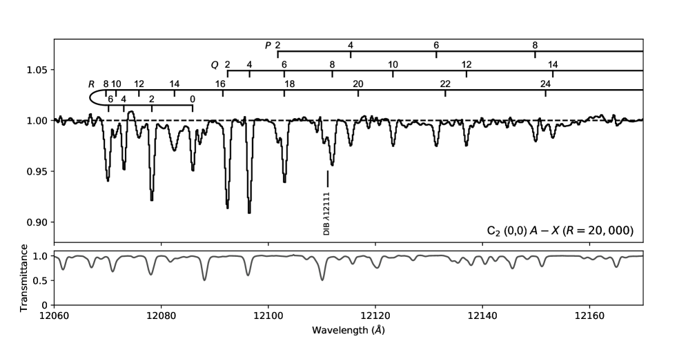
Figure 1: Normalized spectra of the C₂ (1,0) (upper panel) and (0,0) (lower panel) Phillips bands toward Cyg OB2 No 12 obtained with the WIDE mode ($R=20,000$). The normalized spectra of the telluric standard stars are also shown. The wavelengths of each line of the bands are marked with lines above the spectrum. The positions of stellar lines and DIBs (including its candidates) are also shown with lines below the spectrum. The wavelengths of the (1,0) and (0,0) bands were calculated from the wavenumbers listed in table 2 in Chauville et al. (1977) and table 1 in Douay et al. (1988), respectively.

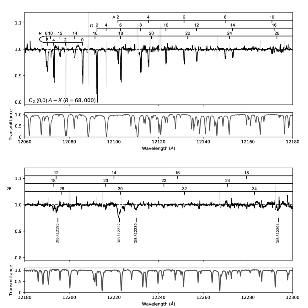
Figure 2: Normalized spectrum of the C₂ (0,0) Phillips band toward Cyg OB2 No. 12 obtained with the HIRES-J mode ($R=68,000$). The wavelength ranges at which the transmittance was lower than 0.5 are plotted with gray lines. The stellar lines and DIBs are also marked with lines below the spectrum. The normalized spectrum of the telluric standard star is also shown.

Figures 1 and 2 show the spectra of C₂ bands obtained with WIDE and HIRES-J modes, respectively. Both the C₂ (0,0) and (1,0) Phillips bands were clearly detected up to the rotational levels of $J^{\prime\prime}>20$ in the ground state for both the WIDE and HIRES-J spectra. The stellar absorption lines and DIBs, with which the C₂ bands are contaminated, are marked in the figures. These DIBs are newly found in this observation and will be reported in another paper (S. Hamano et al. 2019 in preparation). The telluric lines are very weak in the (1,0) band region while the (0,0) band is contaminated with strong telluric absorption lines. The absorption lines of telluric water vapor in the HIRES-J spectrum were particularly strong because the HIRES-J data were obtained in the summer season when the temperature and humidity at the observational site are high. Therefore, as for the HIRES-J data, the wavelength ranges at which the atmospheric transmittance was lower than 0.5 (plotted with gray lines in Figure 2) were not used in the following analysis of the C₂ band.

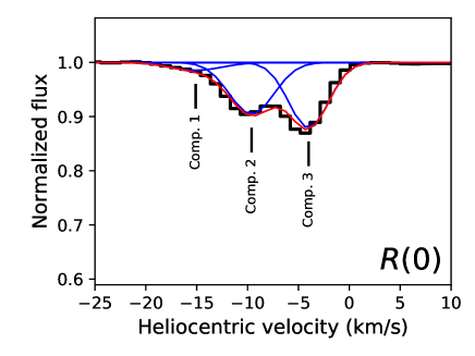
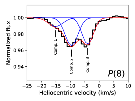
Figure 3: Close-up images of the spectrum of the $R(0)$ and $P(8)$ lines in the C₂ (0,0) band. The black lines show the spectrum of Cyg OB2 No. 12 obtained with the HIRES-J mode. Three components at $-15.1$, $-9.6$, and $-4.0$ km s^-1 were detected. The blue lines show the Gaussian curves fitted to the spectrum. The red lines show the composite of the Gaussian curves.

Figure 3 shows the close-up plots for the $R(0)$ and $P(8)$ lines of the C₂ (0,0) band, which were clearly detected in the HIRES-J spectrum. Three velocity components were resolved with $R=68,000$. In this paper, the three components are referred to as components 1, 2, and 3 as shown in Figure 3. These three components in the line of sight of Cyg OB2 No. 12 were already recognized by McCall et al. (2002) with the CO and K I absorption spectra. They also detected the C₂ (2,0) Phillips band, but could not detect the absorption lines at the velocity of component 1. Components 1, 2, and 3 could not be resolved in our WIDE spectrum ($\Delta v=15$ km s^-1).

We estimated the line-of-sight velocities, Doppler widths, and column densities of each velocity component using VoigtFit (Krogager, 2018), which is a Python package for fitting Voigt profiles to absorption lines. Because the line parameters of C₂ Phillips bands are not included in VoigtFit, we originally calculated the oscillator strengths of each rotational line of C₂ bands. We used the oscillator strengths of $f_{00}=2.233\times 10^{-3}$ and $f_{10}=2.348\times 10^{-3}$ calculated by Schmidt & Bacskay (2007). The oscillator strengths of each line were calculated from the following relation (Gredel et al., 2001):

$$f_{J^{\prime}J^{\prime\prime}}=f_{\text{band}}\frac{\nu_{J^{\prime}J^{\prime\prime}}}{\nu_{\text{band}}}\frac{S_{J^{\prime}J^{\prime\prime}}}{2(2J^{\prime\prime}+1)},$$ (1)

where $f_{\text{band}}$ is the oscillator strength of the band ($f_{00}$ or $f_{10}$), $\nu_{\text{band}}$ is the wavenumber of the vibrational band, and $S_{J^{\prime}J^{\prime\prime}}$ are Hönl-London factors: $(J^{\prime\prime}+2)$, $(2J^{\prime\prime}+1)$, and $(J^{\prime\prime}-1)$ for the $R$, $Q$, and $P$ branches, respectively. The wavelengths of the C₂ (0,0) and (1,0) bands were adopted from Douay et al. (1988) and Chauville et al. (1977), respectively.

The C₂ lines were fitted simultaneously to the HIRES-J spectrum using VoigtFit. The regions contaminated with strong telluric absorption lines were eliminated for the fitting as well as for the estimate of the S/N. The S/N of each pixel was calculated considering the loss of flux by the moderate telluric absorption lines. The C₂ lines blended with other features, such as stellar lines and DIBs, were not included in the fitting.

Table 2 lists the column densities for each velocity component obtained by the fitting. The heliocentric velocities of components 1,2 and 3 were estimated as $-15.1$, $-9.6$, and $-4.0$ km s^-1, respectively. The Doppler widths of each velocity component could be estimated in the fitting because the EWs of the strongest $P$, $Q$, and $R$ lines in the optically thick regime. The Doppler widths of components 1, 2, and 3 were estimated as $2.39\pm 0.42$, $1.47\pm 0.15$ and $0.53\pm 0.06$ km s^-1, respectively. We did not conduct the Voigt profile analysis for the WIDE data because the three velocity components, could not be resolved with $R=20,000$ ($\Delta v=15$ km s^-1). Therefore, we used $N(J^{\prime\prime})$ determined from the HIRES-J data in the following analysis.

According to McCall et al. (2002), who obtained the optical spectrum of Cyg OB2 No. 12 with $R=200,000$, the FWHMs of the C₂ (2,0) band absorption lines were measured to be $3.0\pm 0.2$ and $2.0\pm 0.2$ km s^-1 for components 2 and 3, respectively. Considering the broadening effect by instrumental profiles with $\Delta v=1.5$ km s^-1, the Doppler widths estimated from our fitting, $1.47\pm 0.15$ and $0.53\pm 0.06$ km s^-1 for component 2 and 3, correspond to FWHMs of 2.9$\pm 0.3$ and $1.7\pm 0.1$ km s^-1, respectively, in the $R=200,000$ spectrum. These values were consistent with the directly measured FWHMs by McCall et al. (2002).

The column densities obtained by our analysis were compared with those of Gredel et al. (2001) and McCall et al. (2002), both of which analyzed the spectrum of the (2,0) Phillips band of Cyg OB2 No. 12. Gredel et al. (2001) obtained the spectrum with $R=45,000$ and S/N $>$ 600 and could not resolve the velocity components while McCall et al. (2002) resolved the velocity components with $R=200,000$ but the S/N was not as good as that of Gredel et al. (2001). Although both of them assumed the optically thin conditions for the calculation of column densities considering the typical Doppler width of $b=1$ km s^-1 (Gredel et al., 2001), this assumption is not valid in the case of $b=0.5$ km s^-1. Therefore, we calculated the column densities from the (2,0) band equivalent widths (EWs) by Gredel et al. (2001) and McCall et al. (2002) using the Doppler widths and the velocities estimated from our fitting, and then compared the resultant column densities with those we derived from the (0,0) band. We adopted $f_{20}=1.424\times 10^{-3}$ (Schmidt & Bacskay, 2007) for the calculation. The ratios of the column densities from the (2,0) band to our values from the (0,0) band were calculated up to $J^{\prime\prime}=8$, below which we could detect the absorption lines of the velocity component 1. The ratios of the column density of Gredel et al. (2001) to our value was $0.94\pm 0.15$. The column densities calculated from the data of Gredel et al. (2001) were close to our results but the uncertainties were large. Note that the standard deviation does not include the uncertainties of EWs and Doppler widths. As for McCall et al. (2002), the ratios were calculated to be $0.79\pm 0.07$ and $0.74\pm 0.07$ for components 2 and 3, respectively, meaning that the EWs of McCall et al. (2002) were lower than those expected from the (0,0) band. Considering the relatively low S/N of the McCall et al. (2002) spectrum, the discrepancy could be attributed to the systematic noise, which could not be estimated in their paper (see the footnote of Table 6 in McCall et al., 2002). Also, the systematic uncertainties due to the continuum normalization could be large because the strong lines in the (2,0) band are detected within the broad stellar lines of H I Paschen 12 and He I. Therefore, the column densities obtained from our (0,0) band data could be more robust than the previous results because of both the high quality of our data and intrinsically large EWs of the (0,0) band.

To measure the EWs of the detected lines independently, we fitted Gaussian curves to the spectrum data. The velocities and widths were fixed in the fit as determined by the VoigtFit analysis for the HIRES-J spectrum. For the partially blended lines, multiple Gaussian curves at the wavelengths of the blended lines were fitted simultaneously. While the EWs of the three velocity components were measured separately in the HIRES-J spectrum, the total EWs of the three components were measured in the WIDE spectrum. For the EW uncertainties, we included the systematic uncertainties from continuum fitting estimated with the rms shift method (Sembach & Savage, 1992) in addition to the statistical uncertainties. Tables 2 and 3 list the EWs measured for the absorption lines identified as C₂ Phillips bands in the spectra obtained with the HIRES-J and WIDE modes, respectively. In the WIDE spectrum, the lower spectral resolution caused the blending of some multiple C₂ lines and it made it difficult to normalize the spectrum using the surrounding continuum regions. We did not list the EWs for those lines, whose systematic uncertainties of EWs were much larger due to the blending. In Table 3, we also list the EWs of the (1,0) band calculated from $N(J^{\prime\prime})$ and $b$ determined by HIRES-J data using $f_{10}=2.348\times 10^{-3}$ (Schmidt & Bacskay, 2007). Comparing the measured and calculated EWs, we discuss the ratio of observationally constrained oscillator strengths of Phillips bands in Section 4.2. Note that the total EWs measured from WIDE and HIRES spectra are consistent within uncertainties for the most lines detected in both spectra.

Table 2: Equivalent widths and column densities for the C₂ $(0,0)$ Phillips Bands in the HIRES-J mode spectrum of Cyg OB2 No. 12

				Comp 1			Comp 2			Comp 3
$J^{\prime\prime}$	Branch	$\lambda_{\text{air}}$ (Å)	$f(10^{-3})$	EW (mÅ)	$N$ ($10^{12}$ cm-2)		EW (mÅ)	$N$ ($10^{12}$ cm-2)		EW (mÅ)	$N$ ($10^{12}$ cm-2)	Blending
$0$	$R$	12086.244	2.230	$3.55\pm 0.40$	$0.93\pm 0.21$		$20.55\pm 0.31$	$7.40\pm 0.24$		$23.93\pm 0.33$	$10.83\pm 0.33$
$2$	$R$	12078.631	0.894	$\cdots$	$2.94\pm 0.55$		$\cdots$	$27.25\pm 0.60$		$\cdots$	$39.63\pm 1.66$	Telluric
	$Q$	12092.725	1.120	$5.51\pm 0.41$			$36.13\pm 0.32$			$36.82\pm 0.34$
	$P$	12102.141	0.223	$2.09\pm 0.40$			$8.54\pm 0.31$			$10.81\pm 0.33$
$4$	$R$	12073.398	0.745	$6.47\pm 0.36$	$5.75\pm 0.70$		$24.16\pm 0.28$	$25.69\pm 0.82$		$24.01\pm 0.29$	$30.96\pm 0.74$
	$Q$	12096.879	1.120	$\cdots$			$\cdots$			$\cdots$		Telluric
	$P$	12115.742	0.371	$2.64\pm 0.41$			$10.81\pm 0.33$			$12.56\pm 0.35$
$6$	$R$	12070.540	0.688	$\cdots$	$3.52\pm 0.47$		$15.72\pm 0.32$	$17.90\pm 0.54$		$13.91\pm 0.30$	$20.15\pm 0.47$	$R(8)$
	$Q$	12103.413	1.110	$\cdots$			$\cdots$			$\cdots$		$R(18)$
	$P$	12131.760	0.428	$2.79\pm 0.33$			$9.72\pm 0.26$			$10.60\pm 0.28$
$8$	$R$	12070.055	0.658	$2.47\pm 0.36$	$3.89\pm 0.40$		$10.07\pm 0.28$	$12.46\pm 0.46$		$\cdots$	$12.34\pm 0.29$	$R(6)$
	$Q$	12112.335	1.110	$6.25\pm 0.40$			$17.11\pm 0.31$			$15.29\pm 0.33$
	$P$	12150.211	0.457	$3.03\pm 0.41$			$7.70\pm 0.31$			$6.56\pm 0.33$
$10$	$R$	12071.943	0.639	$\cdots$	$\cdots$		$\cdots$	$9.58\pm 0.40$		$\cdots$	$8.19\pm 0.34$	Telluric
	$Q$	12123.652	1.110	$\cdots$			$13.88\pm 0.27$			$10.52\pm 0.28$
	$P$	12171.114	0.475	$\cdots$			$5.10\pm 0.22$			$4.30\pm 0.23$
$12$	$R$	12076.208	0.626	$5.07\pm 0.35$	$2.26\pm 0.38$		$5.61\pm 0.27$	$7.27\pm 0.39$		$4.66\pm 0.29$	$6.18\pm 0.32$
	$Q$	12137.378	1.110	$2.81\pm 0.34$			$10.20\pm 0.27$			$7.96\pm 0.29$
	$P$	12194.491	0.487	$\cdots$			$\cdots$			$\cdots$		DIB
$14$	$R$	12082.853	0.616	$\cdots$	$1.70\pm 0.34$		$\cdots$	$4.33\pm 0.70$		$\cdots$	$3.78\pm 0.29$	Telluric
	$Q$	12153.526	1.110	$3.14\pm 0.41$			$6.52\pm 0.31$			$5.35\pm 0.33$
	$P$	12220.370	0.495	$\cdots$			$1.98\pm 0.39$			$1.72\pm 0.41$
$16$	$R$	12091.888	0.609	$\cdots$	$\cdots$		$2.48\pm 0.33$	$3.25\pm 0.28$		$1.32\pm 0.33$	$2.01\pm 0.25$
	$Q$	12172.113	1.110	$\cdots$			$4.73\pm 0.22$			$2.95\pm 0.23$
	$P$	12248.774	0.501	$\cdots$			$1.82\pm 0.31$			$1.24\pm 0.34$
$18$	$R$	12103.322	0.603	$\cdots$	$1.24\pm 0.33$		$\cdots$	$2.78\pm 0.32$		$\cdots$	$2.07\pm 0.28$	$Q(6)$
	$Q$	12193.162	1.110	$1.73\pm 0.40$			$4.18\pm 0.30$			$2.73\pm 0.33$
	$P$	12279.735	0.505	$\cdots$			$\cdots$			$\cdots$
$20$	$R$	12117.168	0.598	$\cdots$	$\cdots$		$2.16\pm 0.32$	$2.72\pm 0.26$		$2.88\pm 0.33$	$2.34\pm 0.23$
	$Q$	12216.696	1.100	$\cdots$			$3.59\pm 0.39$			$2.08\pm 0.41$
	$P$	12313.287	0.508	$\cdots$			$2.31\pm 0.22$			$1.55\pm 0.24$
$22$	$R$	12133.443	0.593	$\cdots$	$\cdots$		$\cdots$	$1.94\pm 0.34$		$\cdots$	$\cdots$
	$Q$	12242.736	1.100	$\cdots$			$2.75\pm 0.31$			$\cdots$
	$P$	12349.467	0.510	$\cdots$			$\cdots$			$\cdots$
$24$	$R$	12152.165	0.589	$\cdots$	$\cdots$		$\cdots$	$\cdots$		$\cdots$	$\cdots$	Telluric
	$Q$	12271.315	1.100	$\cdots$			$\cdots$			$\cdots$
	$P$	12388.311	0.511	$\cdots$			$\cdots$			$\cdots$
$26$	$R$	12173.354	0.586	$\cdots$	$\cdots$		$1.36\pm 0.22$	$1.40\pm 0.30$		$0.78\pm 0.23$	$1.36\pm 0.27$
	$Q$	12302.463	1.100	$\cdots$			$1.83\pm 0.22$			$2.07\pm 0.24$
	$P$	12429.866	0.512	$\cdots$			$\cdots$			$\cdots$
$28$	$R$	12197.033	0.582	$\cdots$	$\cdots$		$\cdots$	$\cdots$		$1.35\pm 0.33$	$1.53\pm 0.27$
	$Q$	12336.214	1.090	$\cdots$			$\cdots$			$2.06\pm 0.28$
	$P$	12474.185	0.512	$\cdots$			$\cdots$			$\cdots$

Note. — The symbol ” $\cdots$ ” denotes undetected lines.

Table 3: Equivalent widths for the C₂ (0,0) and (1,0) Phillips Bands in the WIDE-mode spectrum of the Cyg OB2 No. 12

		(0,0)	(1,0)	(1,0) calculation
$J^{\prime\prime}$	Branch	EW (mÅ)	EW (mÅ)	EW (mÅ)
$0$	$R$	$\cdots$	$35.30\pm 1.49$	35.93
$2$	$R$	$66.36\pm 1.27$	$\cdots$	49.57
	$Q$	$75.55\pm 0.89$	$60.35\pm 1.50$	59.54
	$P$	$19.29\pm 0.94$	$\cdots$	14.09
$4$	$R$	$\cdots$	$\cdots$	39.39
	$Q$	$\cdots$	$\cdots$	56.16
	$P$	$23.59\pm 1.12$	$20.49\pm 1.02$	20.87
$6$	$R$	$\cdots$	$\cdots$	25.26
	$Q$	$\cdots$	$41.35\pm 1.49$	39.44
	$P$	$19.78\pm 1.13$	$17.31\pm 1.18$	16.26
$8$	$R$	$\cdots$	$\cdots$	17.17
	$Q$	$\cdots$	$27.26\pm 0.95$	28.47
	$P$	$17.34\pm 0.97$	$12.15\pm 1.09$	12.23
$10$	$R$	$\cdots$	$\cdots$	11.14
	$Q$	$22.26\pm 1.13$	$20.57\pm 1.17$	19.17
	$P$	$\cdots$	$\cdots$	8.48
$12$	$R$	$\cdots$	$\cdots$	9.16
	$Q$	$19.33\pm 1.13$	$13.57\pm 1.09$	16.18
	$P$	$\cdots$	$6.33\pm 0.98$	7.29
$14$	$R$	$\cdots$	$\cdots$	5.69
	$Q$	$11.97\pm 0.96$	$\cdots$	10.28
	$P$	$\cdots$	$\cdots$	4.67
$16$	$R$	$\cdots$	$\cdots$	3.45
	$Q$	$\cdots$	$\cdots$	6.34
	$P$	$\cdots$	$\cdots$	2.90
$18$	$R$	$\cdots$	$5.05\pm 0.97$	3.47
	$Q$	$\cdots$	$\cdots$	6.41
	$P$	$\cdots$	$\cdots$	2.99
$20$	$R$	$3.53\pm 1.12$	$\cdots$	3.18
	$Q$	$\cdots$	$\cdots$	5.92
	$P$	$\cdots$	$\cdots$	2.78

Note. —

3.2 CN red band

Table 4: Equivalent widths and column densities for the CN red bands in the WIDE-mode spectrum of Cyg OB2 No. 12

Band	Transition	$N^{\prime\prime}$	$J^{\prime\prime}$	$\lambda_{\text{air}}$	$f_{\text{osc}}$	EW	$N(N^{\prime\prime})$	$N(N^{\prime\prime})$
				(Å)	($\times 10^{-3}$)	(mÅ)	($10^{12}$ cm-2)	($10^{12}$ cm-2)
(1,0) band	${}^{S}R_{21}(0)$	$0$	$1/2$	9139.699	0.2646	$6\pm 3$	$31\pm 15$	$31\pm 15$
	$R_{2}(1)+^{R}Q_{21}(1)$	$1$	$1/2+3/2$	9142.848	0.4375	$12\pm 3$	$37\pm 9$	$40\pm 10$
	${}^{R}Q_{21}(0)$	$0$	$1/2$	9144.055	0.6409	$17\pm 3$	$36\pm 6$	$38\pm 6$
	$Q_{2}(1)+^{Q}P_{21}(1)$	$1$	$1/2+3/2$	9147.219	0.3203	$\cdots$	$\cdots$	$\cdots$
	$R_{1}(1)$	$1$	$3/2$	9183.230	0.6408	$14\pm 3$	$45\pm 9$	$46\pm 9$
	$R_{1}(0)$	$0$	$1/2$	9186.950	1.0127	$21\pm 3$	$28\pm 4$	$29\pm 4$
	${}^{Q}R_{12}(1)+Q_{1}(1)$	$1$	$1/2+3/2$	9190.138	0.5851	$20\pm 3$	$46\pm 7$	$50\pm 8$
(0,0) band	${}^{S}R_{21}(0)$	$0$	$1/2$	10925.147	0.3251	$10\pm 2$	$29\pm 6$	$29\pm 6$
	$R_{2}(1)+^{R}Q_{21}(1)$	$1$	$1/2+3/2$	10929.650	0.5386	$\cdots$	$\cdots$	$\cdots$
	${}^{R}Q_{21}(0)$	$0$	$1/2$	10931.442	0.7892	$\cdots$	$\cdots$	$\cdots$
	${}^{Q}P_{21}(1)+Q_{2}(1)$	$1$	$1/2+3/2$	10935.970	0.3945	$\cdots$	$\cdots$	$\cdots$
	$R_{1}(1)$	$1$	$3/2$	10987.395	0.7886	$17\pm 2$	$30\pm 3$	$33\pm 3$
	$R_{1}(0)$	$0$	$1/2$	10992.869	1.2461	$74\pm 2$	$55\pm 2$	$67\pm 3$
	$Q_{1}(1)+^{Q}R_{12}(1)$	$1$	$1/2+3/2$	10997.445	0.7198	$\cdots$	$\cdots$	$\cdots$

Note. —

Figure 4 shows the WIDE spectra of the CN (1,0) and (0,0) red bands. The rest-frame wavelengths were adopted from Brooke et al. (2014). As shown in Figure 4, some absorption lines were detected at the wavelengths of CN bands. In particular, the three lines of the (0,0) band around $\lambda=$ 10990 Å were clearly detected. As long as we know, this is the first detection of a (0,0) band of the CN red system in the interstellar medium. The lines around 10930Å are overlapped with the broad absorption line of H I Pa$\gamma$. Within the broad feature of the stellar H I line, narrow dips can be seen at the wavelengths of the CN band. These dips are most likely CN lines, but it is almost impossible to measure their EWs accurately. Table 4 lists the EWs and column densities measured for the lines of the CN (1,0) and (0,0) red bands in the spectrum of Cyg OB2 No. 12. The EWs were measured by fitting a Gaussian curve to the spectrum. Although these CN lines should originate from two major velocity components, components 2 and 3, as well as C₂, they could not be resolved. The measured EWs would be the sum of all velocity components.

Considering the small Doppler widths measured from the C₂ (0,0) band, some detected CN lines are probably optically thick. However, since we could not resolve the velocity components, we could not estimate the Doppler widths of each velocity component. Therefore, we calculated CN column densities based on two assumptions. One is the assumption of the optically thin condition and the other is the assumption that the CN lines that originated from components 1, 2 and 3 and have the same Doppler widths as the C₂ lines. In the latter assumption, the ratios of column densities of each velocity component to the total column densities were assumed as those of the C₂ column densities. The oscillator strengths calculated by Brooke et al. (2014) were adopted. For the blended lines from the $N^{\prime\prime}=1$ level, we calculated the effective oscillator strengths by assuming that the populations of the spin-rotational levels $(N^{\prime\prime},J^{\prime\prime})$ with the same rotational quantum number $N^{\prime\prime}$ are populated according to their statistical weights (Gredel, et al., 2002). Table 4 lists the column densities calculated under two assumptions. As for the $R_{1}(0)$ line of the CN (0,0) band, which is the strongest detected line, the column density was much different by the assumptions. The column densities of the $N^{\prime\prime}=0$ and 1 levels estimated from each line, $N(N^{\prime\prime}=0)$ and $N(N^{\prime\prime}=1)$, have larger variance than the uncertainties (Table 4). This would be because of the systematic uncertainties due to the surrounding stellar lines, which made it difficult to properly evaluate the appropriate continuum level. Also, both bands were severely contaminated by telluric absorption lines.

The (2,0) and (1,0) bands of the CN red system toward Cyg OB2 No. 12 were also detected by Gredel et al. (2001). As for the (1,0) band, which was also detected in this study, Gredel et al. (2001) showed that the EWs of $Q_{2}(1)+^{Q}P_{21}(1)$ and $R_{1}(0)$ were $14.3\pm 5$Å and $25\pm 5$Å, respectively, and the EW upper limits of ${}^{S}R_{21}(0)$ and $R_{1}(1)$ were $<28$Å and $<53$Å, respectively. The EWs and upper limits of the (1,0) band measured here were consistent with those reported by Gredel et al. (2001) within uncertainties.

Averaging the column densities calculated with the optically thin condition assumption listed in Table 4, the column densities of the $N^{\prime\prime}=0$ and 1 levels were estimated to be $N(N^{\prime\prime}=0)=(4.7\pm 0.2)\times 10^{13}$ and $N(N^{\prime\prime}=1)=(3.2\pm 0.3)\times 10^{13}$ cm^-2. The rotational excitation temperature and the CN total column density were estimated to be $T_{10}=3.7\pm 0.3$ K and $N(\text{CN})=(8.2\pm 0.4)\times 10^{13}$ cm^-2. Note that these results are likely to be affected by the systematic uncertainties due to the residual of telluric absorption lines and the stellar lines.

Using only the $R_{1}(0)$ and $R_{1}(1)$ lines of the CN (0,0) band, which were clearly detected without the contamination of stellar lines, we estimated the rotational excitation temperature and the CN total column density to be $T_{10}=3.0\pm 0.2$ K and $N($CN$)=(1.01\pm 0.04)\times 10^{14}$ cm^-2, respectively, in the optically thick case for the $R_{1}(0)$ and $R_{1}(1)$ lines of CN (0,0) band. We suggest that the latter result would be more robust because the rotational temperature is close to the CMB temperature. Gredel et al. (2001) estimated $N(N^{\prime\prime}=0)=4.4\times 10^{13}$ and $N(N^{\prime\prime}=1)=5.5\times 10^{13}$ cm^-2 (the oscillator strength was adjusted to the values of Brooke et al. 2014 for comparison). Our result should be more robust than that of Gredel et al. (2001) since the $N(N^{\prime\prime}=1)$ by Gredel et al. (2001) had a large uncertainty and their excitation temperature, $T_{10}=6.2$ K, was much higher than the CMB temperature. However, there is a systematic uncertainty in our results due to the assumption about the Doppler widths and the CN column density ratios among velocity components. It is necessary to resolve the velocity components with higher resolution and detect more lines to obtain these parameters with high accuracy.

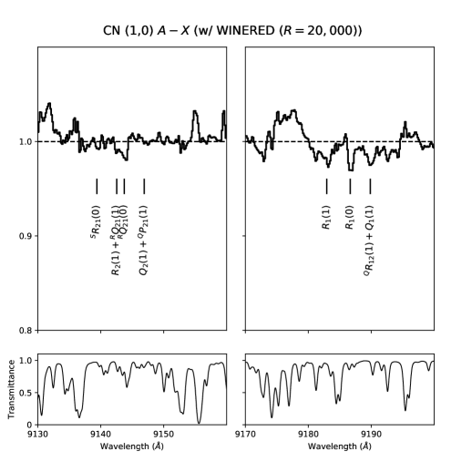
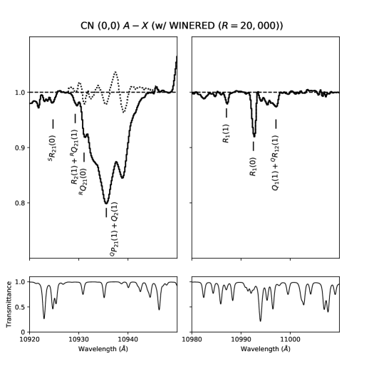
Figure 4: The left two panels and right two panels show the spectra of the CN (1,0) and (0,0) red bands toward Cyg OB2 No. 12, respectively. The transmittance spectrum synthesized using ATRAN (Lord, 1992) is also shown, in the lower panels. The wavelengths of the CN red system are adopted from Brooke et al. (2014). The dotted line shows the spectrum after subtracting the Gaussian function arbitrarily fitted to the Pa $\gamma$ line.

4 Discussion

4.1 Rotational excitation of C₂

The gaseous temperature and density of the collision partner ($n(\text{H})+n(\text{H}_{2})$) can be evaluated from the rotational distribution of C₂ molecules. These parameters are essential for understanding of the interstellar chemical reactions (Gredel et al., 2001). Using the model of van Dishoeck & Black (1982), we estimated the parameters for the three velocity components of Cyg OB2 No. 12 from the column densities of each rotational level in the ground state. We use the updated value of the absorption rates calculated by van Dishoeck & de Zeeuw (1984). We assumed the scaling factor for the incident radiation field to be $I=1$. As the recent analysis of interstellar C₂ excitation by Hupe et al. (2012), we adopted the C₂-H₂ collisional cross section as $\sigma_{0}=4\times 10^{-16}$ cm^-2, which is indicated by recent calculations (Lavendy et al., 1991; Robbe et al., 1992; Najar et al., 2008, 2009), rather than the frequently used value of $2\times 10^{-16}$ cm^-2 (van Dishoeck & Black, 1982). Although the lines from $J^{\prime\prime}>20$ were detected in our observation, the original model by van Dishoeck & Black (1982) cannot predict the rotational distributions at $J^{\prime\prime}>20$, because they calculated the radiation excitation matrix and the quadruple transition probabilities up to only $J^{\prime\prime}=20$. To extrapolate the model to $J^{\prime\prime}>20$, we estimated the values of the model parameters at $J^{\prime\prime}>20$ levels by fitting power-law functions of $J^{\prime\prime}$, which reproduced the values at $J^{\prime\prime}\leq 20$ well.

Figure 5 shows the rotational diagrams for each velocity component. The HIRES-J data were used. We could not estimate the parameters for component 1 because of the large uncertainties of column densities. For components 2 and 3, the kinetic temperatures and gas densities $(T,n)$ were estimated as $(30\pm 5$ K, $100\pm 7$ cm${}^{-3})$ and $(25\pm 5$ K, $125\pm 7$ cm${}^{-3})$, respectively. We compare these results with the previous results of C₂ for Cyg OB2 No. 12 (Gredel et al., 2001; McCall et al., 2002). Because both of the previous papers used the collisional cross section of $2\times 10^{-16}$ cm^-2, which is the half of our adopted value, their densities were scaled by a factor of about 2 for the comparison in the following. McCall et al. (2002) estimated the parameters to be (40 K , 110 cm^-3) and (30 K, 105 cm^-3) for components 2 and 3, respectively, but with large uncertainties: $T=25-55$ K and $n=75-300$ cm^-3 (3$\sigma$ errors). Gredel et al. (2001) analyzed the rotational distribution summed over the components and estimated the parameters to be $(T,n)=(35$ K, $150\pm 25$ cm^-3). They detected the lines of the C₂ (2,0) band up to $J^{\prime\prime}=18$ but could not resolve the velocity components. In comparison with the previous results, both parameters estimated in this paper are consistent with the previous values within uncertainties. Because of the higher oscillator strength of the C₂ (0,0) band than the C₂ (2,0) band, we could estimate the parameters with an accuracy higher than that of previous studies, even those with similar S/Ns.

From the rotational distribution, the C₂ total column densities of components 2 and 3 were estimated to be $(1.29^{+0.16}_{-0.10})\times 10^{14}$ and $(1.48^{+0.13}_{-0.08})\times 10^{14}$ cm^-2, respectively. By summing up the column densities listed in Table 2, the C₂ total column densities of components 1, 2, and 3 were $2.2\times 10^{13}$, $1.2\times 10^{14}$ and $1.4\times 10^{14}$ cm^-2, respectively. Table 5 summarizes the parameters of the velocity components of Cyg OB2 No. 12 obtained from the C₂ and CN bands.

Table 5: Summary of parameters

Comp.	$v$	$b$	$N_{\text{obs}}$(C2)	$N_{\text{calc}}$(C2)	$T_{\text{rot}}$(C2)	$n$(C2)	$N_{J^{\prime\prime}=0}$(CN)	$N_{J^{\prime\prime}=1}$(CN)	$T_{\text{rot}}$(CN)	$N$(CN)
	(km s-1)	(km s-1)	($10^{12}$ cm-2)	($10^{12}$ cm-2)	(K)	(cm-3)	($10^{12}$ cm-2)	($10^{12}$ cm-2)	(K)	($10^{12}$ cm-2)
1	$-15.1$	$2.39\pm 0.42$	$22$	$\cdots$	$\cdots$	$\cdots$	$\cdots$	$\cdots$	$\cdots$	$\cdots$
2	$-9.6$	$1.47\pm 0.15$	$120$	$129^{+16}_{-10}$	$30\pm 5$	$100\pm 7$	$\cdots$	$\cdots$	$\cdots$	$\cdots$
3	$-4.0$	$0.53\pm 0.06$	$140$	$148^{+13}_{-8}$	$25\pm 5$	$125\pm 7$	$\cdots$	$\cdots$	$\cdots$	$\cdots$
Sum	$\cdots$	$\cdots$	282	$\cdots$	$\cdots$	$\cdots$	$67\pm 3$	$33\pm 3$	$3.0\pm 0.2$	$101\pm 4$

Note. — The values are in units of 10¹² cm^-2.

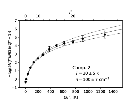
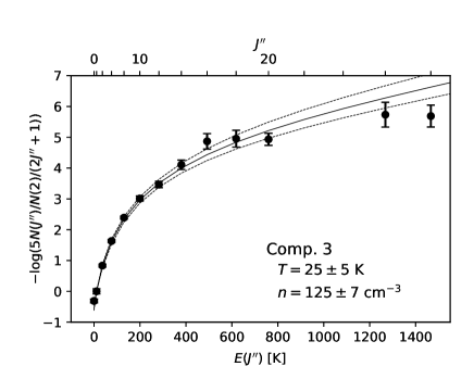
Figure 5: The rotational diagrams for components 2 (upper panel) and 3 (lower panel). Best-fit model lines and its one sigma ranges are plotted with the solid and dashed lines, respectively.

4.2 Oscillator strengths

The oscillator strengths of the C₂ Phillips bands have been investigated experimentally and theoretically. However, the experimental and theoretical results are not in agreement with one another. Astronomical observations of C₂ molecules have put a unique constraint on the oscillator strength ratios of C₂ bands (Lambert et al., 1995). Here, we try to put constraints on the oscillator strength ratios of the C₂ Phillips bands of Cyg OB2 No.12 using the line strengths of (1,0) and (0,0) bands from this study. We use the (0,0) band in HIRES spectrum and the (1,0) band in WIDE spectrum. It is assumed that the column densities of rotational levels $J^{\prime\prime}$ in the line of sight of Cyg OB2 No. 12 are constant between our observations with WIDE and HIRES-J modes. From the strength ratios between the detected lines of (1,0) and (0,0) bands from the same lower level $J^{\prime\prime}$, the oscillator strength ratio, $f_{00}/f_{10}$, can be constrained.

Because the strong lines of Cyg OB2 No. 12 are optically thick for both (0,0) and (1,0) bands (§3.1), the oscillator strength ratio cannot be simply calculated from the ratio of the EWs. Therefore, we searched for the oscillator strength ratio that reproduces well the observed EWs with the following procedures. First, we calculated the total EWs of the three velocity components for each rotational lines of the (1,0) band by synthesizing the absorption profiles using the column densities of each rotational level listed in Table 2 and the cloud parameters (the line-of-sight velocities and Doppler widths), which were determined from the (0,0) band (Table 3). By varying the oscillator strength of the (1,0) bands from $f_{10}=2.348\times 10^{-3}$ (Schmidt & Bacskay, 2007) in the calculation, we searched for the best value of $f_{10}$ reproducing the observed EWs of the (1,0) band. As a result, the $f_{00}/f_{10}$ was estimated to be $0.96\pm 0.05$.

The ratios were compared with the experimental results (Davis, et al., 1984; Bauer, et al., 1985) and calculated values (Schmidt & Bacskay, 2007) in Table 6. Although the obtained ratio is closer to the theoretical result than the experimental result, it is consistent with both the experimental and theoretical results within the 1$\sigma$ uncertainty. High-resolution data that can resolve the velocity components will be necessary for both bands in order to put stronger constraints on the oscillator strength ratios. The oscillator strength constraints from astronomical data can contribute to future improvements of the C₂ estimate (not only for the oscillator strengths of relevant bands of C₂, but also for astrophysical measurements).

Table 6: Oscillator strengths of C₂ Phillips bands

Reference	Method	$f_{00}\times 10^{3}$	$f_{10}\times 10^{3}$	$f_{00}/f_{10}$
Davis, et al. (1984)	Experiment	$1.38\pm 0.14$	$1.70\pm 0.17$	$0.81\pm 0.11$
Bauer, et al. (1985)	Experiment	1.38	1.56	0.89
Schmidt & Bacskay (2007)	Calculation	2.233	2.348	0.951
This study	Astronomy	$\cdots$	$\cdots$	$0.96\pm 0.05$

4.3 Marginal detection of ¹²C¹³C

We searched for the lines of the ¹²C¹³C (0,0) Phillips band in the HIRES-J spectrum. The wavelengths were based on the wavenumbers measured by Amiot & Verges (1983). ¹²C¹³C has the rotational levels of both odd and even rotational quantum numbers $J^{\prime\prime}$ in the ground state in contrast to ¹²C₂, which has only even numbers of $J^{\prime\prime}$ due to the homonuclear molecule nature. As the expected strengths of the $P$ lines were too weak to be detected, only the $Q$ and $R$ lines were searched. The wavelengths of the ¹²C¹³C lines are distributed in the range of almost the same wavelength range of ¹²C₂. Although the ¹²C¹³C (1,0) Phillips band and the ¹³C¹⁴N (0,0) and (1,0) red bands covered in the WIDE spectrum were also searched using the line lists from Amiot & Verges (1983) and Sneden et al. (2014), respectively, we could not detect any absorption lines of these bands or put meaningful constraints on the isotope ratio.

As a result, only $Q(3)$ lines were marginally detected at the velocities of components 2 and 3. To date, the ¹²C¹³C molecule has never been detected in the interstellar medium. Figure 6 shows the spectrum of the $Q(3)$ lines of ¹²C¹³C. Their EWs were $1.0\pm 0.3$ and $0.7\pm 0.3$ mÅ for components 2 and 3, respectively. Although these dips were very weak, the velocities matched with those of components 2 and 3 for the ¹²C₂ lines. Other $Q$ and $R$ lines are expected to be weaker or contaminated with telluric absorption lines and ¹²C₂ lines; thus, the $Q(3)$ line is the most detectable line in our spectrum of Cyg OB2 No. 12. The multiple line detection for ¹²C¹³C requires higher S/Ns for this target.

From the EWs of $Q(3)$ lines, we estimated the abundance of ¹²C¹³C molecules. We assumed that the oscillator strength and the rotational distribution of ¹²C¹³C in the ground state are the same as ¹²C₂. In contrast to ¹²C₂, ¹²C¹³C can have pure rotational electric dipole transitions, which can cool down the rotational populations of ¹²C¹³C, as they have very weak permanent electric dipole moment. We do not have any information regarding the rotational distribution of ¹²C¹³C, and thus we ignore the pure rotational electric dipole transition of ¹²C¹³C. Because the probability is estimated to be very low (Krishna Swamy, 1987), the difference of rotational distributions between ¹²C₂ and ¹²C¹³C would not be so large. However, note that Bakker & Lambert (1998), who detected the ¹²C¹³C absorption band in a circumstellar shell, found that the lower rotational excitation temperature of ¹²C¹³C, compared with that of ¹²C₂, is probably due to the radiative cooling of ¹²C¹³C by the pure rotational electric dipole transition.

On the basis of these assumptions, the ¹²C₂ / ¹²C¹³C ratios for Cyg OB2 No. 12 were estimated to be $\sim 25$ and $\sim 50$ for components 2 and 3, respectively. Conversion of these values into carbon isotope ratios results in ¹²C / ¹³C $\sim 50$ and $\sim 100$, respectively. Considering the large uncertainties in the EWs, this is roughly consistent with the carbon isotope ratios in the interstellar medium measured by various carbon molecules: $68\pm 15$ at the solar galactocentric distance (measurements of CO, CN, and H₂CO in Milam et al., 2005) and $76\pm 2$ in the local ISM (CH⁺ measurement in Stahl et al., 2008). In addition to the EW uncertainties, the deviation of the ¹²C¹³C rotational distribution from that of ¹²C₂, which was assumed here, can cause additional uncertainties in the resultant carbon isotope ratio. By taking higher-quality spectra and detecting multiple rotational lines (especially those arising from different rotational levels), the carbon isotope ratios of C₂ molecules can be investigated more accurately. Bakker & Lambert (1998) suggested that the isotopic exchange reaction of C₂ molecules is too slow to alter the ¹²C₂ / ¹²C¹³C ratio. The observation of ¹²C₂ and ¹²C¹³C will give us new information about the interstellar carbon isotope ratio and related chemical processes in the regime of translucent clouds.

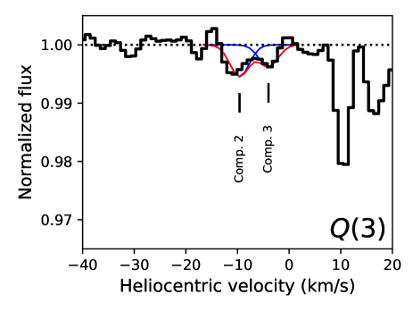
Figure 6: Spectrum of the ¹²C¹³C $Q(3)$ line. The weak absorption lines were detected at the velocities of components 2 and 3. The absorption lines seen at about +10 and +16 km s^-1 are the ¹²C₂ $R(16)$ lines of the components 2 and 3, respectively.

5 Summary

We reported the first detection of the C₂ (0,0) Phillips band and the CN (0,0) red band in the interstellar medium. We obtained the NIR high-resolution spectrum of Cyg OB2 No. 12 using the WINERED spectrograph mounted on the 1.3 m Araki telescope in Kyoto, Japan. We could detect the (0,0) and (1,0) bands of C₂ and CN with high S/N. In particular, the velocity components were clearly resolved in the C₂ (0,0) band spectrum ($R=68,000$). Our findings are summarized as follows:

1. The CN column densities at levels of $N^{\prime\prime}=0$ and 1 were estimated to be $(6.7\pm 0.3)\times$ 10¹³ and $(3.3\pm 0.3)\times$ 10¹³ cm^-2, respectively. From the ratio, the rotational excitation temperature and the CN total column density were calculated as $T_{10}=3.7\pm 0.3$ K and $N(CN)=(8.2\pm 0.4)\times 10^{13}$ $T_{10}=3.0\pm 0.2$ K and $N(CN)=(1.01\pm 0.04)\times 10^{14}$ cm^-2, respectively.

2. From the rotational distribution of C₂, the temperatures and densities, $(T,n)$, of components 2 and 3 were estimated to be $(30\pm 5$ K, $100\pm 7$ cm${}^{-3})$ and $(25\pm 5$ K, $125\pm 7$ cm${}^{-3})$, respectively. These essential physical parameters for understanding the interstellar chemistry could be estimated with high accuracy, due to the large oscillator strength of the (0,0) band, which allowed us to detect the rotational lines from high rotational levels for each velocity component.

3. From the line ratios between the C₂ (0,0) and (1,0) Phillips bands, the oscillator strength ratio, $f_{00}/f_{10}$, of the Phillips bands were constrained. The ratio is estimated to be $f_{00}/f_{10}=0.96\pm 0.05$, which is consistent with both theoretical and experimental values within 1$\sigma$ uncertainties. In order to put stronger constraints on $f_{00}/f_{10}$ from the astronomical observations, it is necessary to obtain high-resolution spectra, in which the velocity components are resolved for both bands.

4. We marginally detected the $Q(3)$ lines of ¹²C¹³C at the velocities of components 2 and 3. If these lines are real, this is the first detection of ¹²C¹³C in the interstellar medium. Assuming that the oscillator strength and rotational distributions of ¹²C¹³C are the same as those of ¹²C₂, the carbon isotope ratio was estimated to be 50–100, which is roughly consistent with the values in the local interstellar medium measured from other carbonaceous molecular features.

In this paper, we demonstrated that the absorption bands of C₂ and CN in the NIR region can be used to investigate the physical properties of interstellar clouds. Thanks to the large oscillator strengths of these NIR bands, we could improve the accuracy of the physical parameters estimated from the rotational distributions of both C₂ and CN. On the other hand, the strong telluric absorption lines that overlapped with the NIR bands make the analysis complicated and increase the systematic uncertainties. The removal of telluric absorption lines is critical for analyzing these NIR bands. Along with observational improvements, the updated model of C₂ excitation (Casu & Cecchi-Pestellini, 2012) is also important for extracting further information regarding interstellar clouds. In addition to these absorption features of small carbonaceous molecules, many DIBs, which are considered to originate from large carbonaceous molecules such as fullerenes and PAHs, have been found in the $Y$ and $J$ bands covered in our observation (Cox et al., 2014; Hamano et al., 2015, 2016). In particular, the DIBs recently identified as absorption features of C${}_{60}^{+}$ are located at about 9600Å. In view of the richness of important molecular features, the wavelength range of the $Y$ and $J$ bands is crucial to the study of interstellar carbon chemistry in diffuse clouds. In the future, it will be important to investigate the relationship between DIBs (including C${}_{60}^{+}$ features), the abundances of C₂ and CN and the physical parameters of interstellar clouds (Elyajouri et al., 2018).

References

- Amiot & Verges (1983) Amiot, C., & Verges, J. 1983, A&AS, 51, 257
- Bakker & Lambert (1998) Bakker, E. J. & Lambert, D. L. 1998, ApJ, 508, 387.
- Bauer, et al. (1985) Bauer, W., Becker, K. H., Hubrich, C., et al. 1985, ApJ, 296, 758.
- Brooke et al. (2014) Brooke, J. S. A., Ram, R. S., Western, C. M., et al. 2014, ApJS, 210, 23
- Casu & Cecchi-Pestellini (2012) Casu, S., & Cecchi-Pestellini, C. 2012, ApJ, 749, 48
- Chauville et al. (1977) Chauville, J., Maillard, J. P., & Mantz, A. W. 1977, Journal of Molecular Spectroscopy, 68, 399
- Cox et al. (2014) Cox, N. L. J., Cami, J., Kaper, L., et al. 2014, A&A, 569, A117
- Davis, et al. (1984) Davis, S. P., Pecyner, R., Smith, W. H., et al. 1984, ApJ, 287, 455.
- Douay et al. (1988) Douay, M., Nietmann, R., & Bernath, P. F. 1988, Journal of Molecular Spectroscopy, 131, 250
- Elyajouri et al. (2018) Elyajouri, M., Lallement, R., Cox, N. L. J., et al. 2018, A&A, 616, A143
- Gredel et al. (2001) Gredel, R., Black, J. H., & Yan, M. 2001, A&A, 375, 553
- Gredel, et al. (2002) Gredel, R., Pineau des Forêts, G. & Federman, S. R. 2002, A&A, 389, 993.
- Hamano et al. (2015) Hamano, S., Kobayashi, N., Kondo, S., et al. 2015, ApJ, 800, 137
- Hamano et al. (2016) Hamano, S., Kobayashi, N., Kondo, S., et al. 2016, ApJ, 821, 42
- Hupe et al. (2012) Hupe, R. C., Sheffer, Y., & Federman, S. R. 2012, ApJ, 761, 38
- Ikeda et al. (2016) Ikeda, Y., Kobayashi, N., Kondo, S., et al. 2016, Proc. SPIE, 9908, 99085Z
- Krishna Swamy (1987) Krishna Swamy, K. S. 1987, MNRAS, 224, 537.
- Krogager (2018) Krogager, J.-K. 2018, arXiv:1803.01187
- Lambert et al. (1995) Lambert, D. L., Sheffer, Y., & Federman, S. R. 1995, ApJ, 438, 740
- Lavendy et al. (1991) Lavendy, H., Robbe, J. M., Chambaud, G., Levy, B., & Roueff, E. 1991, A&A, 251, 365
- Lord (1992) Lord, S. D. 1992, NASA Technical Memorandum 103957
- Meyer & Jura (1985) Meyer, D. M., & Jura, M. 1985, ApJ, 297, 119
- McCall et al. (2002) McCall, B. J., Hinkle, K. H., Geballe, T. R., et al. 2002, ApJ, 567, 391
- Milam et al. (2005) Milam, S. N., Savage, C., Brewster, M. A., Ziurys, L. M., & Wyckoff, S. 2005, ApJ, 634, 1126
- Najar et al. (2008) Najar, F., Ben Abdallah, D., Jaidane, N., & Ben Lakhdar, Z. 2008, Chemical Physics Letters, 460, 31
- Najar et al. (2009) Najar, F., Ben Abdallah, D., Jaidane, N., et al. 2009, J. Chem. Phys., 130, 204305
- Otsubo et al. (2016) Otsubo, S., Ikeda, Y., Kobayashi, N., et al. 2016, Proc. SPIE, 9908, 990879
- Ritchey et al. (2011) Ritchey, A. M., Federman, S. R., & Lambert, D. L. 2011, ApJ, 728, 36
- Robbe et al. (1992) Robbe, J. M., Lavendy, H., Lemoine, D., & Pouilly, B. 1992, A&A, 256, 679
- Sameshima et al. (2018) Sameshima, H., Matsunaga, N., Kobayashi, N., et al. 2018, PASP, 130, 074502
- Schmidt & Bacskay (2007) Schmidt, T. W., & Bacskay, G. B. 2007, J. Chem. Phys., 127, 234310
- Sembach & Savage (1992) Sembach, K. R., & Savage, B. D. 1992, ApJS, 83, 147
- Sneden et al. (2014) Sneden, C., Lucatello, S., Ram, R. S., Brooke, J. S. A., & Bernath, P. 2014, ApJS, 214, 26
- Snow & McCall (2006) Snow, T. P., & McCall, B. J. 2006, ARA&A, 44, 367
- Souza & Lutz (1977) Souza, S. P., & Lutz, B. L. 1977, ApJ, 216, L49
- Stahl et al. (2008) Stahl, O., Wade, G., Petit, V., Stober, B., & Schanne, L. 2008, A&A, 487, 323
- van Dishoeck & Black (1982) van Dishoeck, E. F., & Black, J. H. 1982, ApJ, 258, 533
- van Dishoeck & de Zeeuw (1984) van Dishoeck, E. F., & de Zeeuw, T. 1984, MNRAS, 206, 383
- Whittet (2015) Whittet, D. C. B. 2015, ApJ, 811, 110
- Yoshikawa et al. (2012) Yoshikawa, T., Ikeda, Y., Fujishiro, N., et al. 2012, Proc. SPIE, 8444, 84456