Modification of the laws of gravity in the DGP model by the presence of a second DGP brane

Abstract

We investigate how the laws of gravity change in the DGP model, if we add a second, parallel 3-brane, endowed with a localized gravitational curvature term. We calculate the gravitational potential energy between two static point sources localized on different branes. We discover a new length scale, which is equal to the geometric mean of the DGP cross-over scale and the separation of the two branes in the extra dimension. For distances, which are larger than this new length scale, we recover the original DGP result, but for smaller distances the gravitational potential is weaker. Furthermore, a region emerges, where a 4-dimensional observer measures a distance independent force. We discuss a possible application of the present scenario for deriving rotation curves of low surface brightness galaxies. Using the Kaluza-Klein description, we observe a curious pattern, in which even and odd KK-modes contribute to the attractive and repulsive parts of the gravitational potential, respectively. Finally, since this setup allows for the existence of a sector of particle species that are interacting arbitrarily weakly with ”our” sector, we discuss the implications of this phenomenon for black holes and the bound on the number of species. We find that the behavior is qualitatively different from theories with a normalizable zero-mode graviton.

1 Introduction

We investigate a particular setup in the braneworld scenario, where two flat (tensionless), parallel 3-branes are embedded in a 4+1-dimensional Minkowski spacetime, where the extra dimension is infinite. Apart from the addition of the 2nd brane, the scenario, which we are considering here, is the same as in Ref. dvali20004d, where the original DGP model was proposed. In the DGP model, there is a 5-dimensional (5-d) bulk theory, consisting of the 5-d Einstein-Hilbert action with the fundamental Planck mass $M_{*}$, and an embedded, tensionless 3-brane, which is endowed with a 4-d Einstein-Hilbert action with the observed Planck mass $M_{\text{P}}$:

$$S=M_{*}^{3}\int\mathrm{d}^{4}x\,\mathrm{d}y\,\sqrt{|G|}\mathcal{R}_{5}+M_{\textnormal{P}}^{2}\int\mathrm{d}^{4}x\,\sqrt{|g|}R,$$ (1)

where $y$ is the coordinate of the extra dimension, $|G|$ is the determinant of the bulk metric, $\mathcal{R}_{5}$ is the bulk Ricci scalar and $|g|$ (with $g_{\mu\nu}(x^{\mu})=G_{AB}(x^{\mu},y=0)$) and $R$ are the respective quantities on the brane. Due to the localized curvature term (the second term in (1)), the phenomenology of the DGP model is quite distinctive: Gravity behaves as 5-dimensional for distances above the cross-over scale $r_{c}\equiv\frac{M_{\textnormal{P}}^{2}}{M_{*}^{3}}$, but changes the regime to 4-dimensional behavior for distances below $r_{c}$. We focus on the gravity part of the model, although a localized matter action in (1) is assumed, which contains the Standard Model (SM) fields.

Setups with parallel branes are interesting in several respects: One example is brane inflation dvali1999brane. In that scenario, inflation in our universe could have been caused by a relative motion between branes. Another example was given in Ref. Dvali:1999gf, where it was suggested that (anti-)baryons could be transported to such a parallel brane leading to a new mechanism of baryogenesis on our brane.

The goal of the present paper is to show how the physical implications of the DGP model are modified, if there exists a 2nd brane with a localized curvature term. In order to study this, we will use a somewhat simplified model, explained in detail in Section 2, and calculate the gravitational potential energy between two static point sources localized on the opposite, parallel branes (in Section 3). We will find that the 2nd brane enhances the effects of the DGP model by further weakening the 5-d gravity at certain distances. Furthermore, we will discover that the resulting gravitational potential gives rise to a potentially, phenomenologically interesting new distance independent force in our universe.

Typically, in the context of extra dimensional models, the Kaluza-Klein (KK) language is adopted, where the presence of the (geometrical) extra dimension is traded for the presence of a tower of KK-modes, seen by a 4-d observer. Although such a viewpoint is usually used in the case of a compact extra dimension (since in that case, one gets a discrete mass spectrum), in Section 4 we will also make use of this KK language and re-derive our results obtained in the fully 5-d treatment. Besides encountering some interesting features, this equivalent viewpoint will serve as a cross-check for our main result.

Finally, we wish to address the question, what are the implications on the present scenario coming from black hole (BH) physics. For general relativity (GR), or theories that behave like GR up to some distance $l_{*}$, it has been shown Dvali2007; Dvali2007a; Dvali2008 that BH physics (with a BH size smaller than $l_{*}$) puts a consistency bound on the short distance cutoff of GR, namely

$$\Lambda\lesssim\frac{M_{\textnormal{P}}}{\sqrt{N}},$$ (2)

where $\Lambda$ is the gravity cutoff and $N$ is the number of species in the theory. The physical meaning of expression (2) is that the parameter $\Lambda^{-1}$ marks the lower bound on the scale of breakdown of semi-classical gravity. For example, the Hawking radiation from a black hole of the size smaller than this scale cannot be treated as thermal, even approximately. This is a clear signal that the theory of general relativity requires a UV-completion at distances shorter than $\Lambda^{-1}$.

Furthermore, it has been shown in the context of an ADD-type model Dvali2008c (see also Dvali2008e; Aryal1986; Achucarro1995) that several setups with multiple branes, where a BH does not intersect with all of the branes, are classically not static. It was shown that there is a classical time scale, until which the BH will ”accrete” all of the other branes. According to Ref. Dvali2008c, in the language of species, this can be understood as a ”democratization” process for the BH in the following sense: A semi-classical, thermal, BH should evaporate into all species ”democratically” (up to greybody factors). However, as long as the BH does not intersect certain branes, it cannot evaporate into the species localized on them. So the process of brane accretion restores that evaporation universality. In this view, the lack of time-independence in the setup is reflected by the lack of universal evaporation.

However, theories of the form considered in the present work, differ from other extra dimensional models (like the ADD model arkani1998hierarchy or the RS model Randall1999; Randall1999a) in a very important aspect: they modify gravity at large distances, while coinciding with GR at short distance scales. Moreover, as opposed to the above outlined ”accretion” scenario, where the tension of the branes is responsible for the attraction between the BH and the branes, in our setup the branes are tensionless. Nevertheless, we will show that there would be an (repulsive) interaction between a BH and the branes. We can, however, switch that interaction off by sending the distance between the branes to infinity. This is not possible in the ADD model, because in that case we would need to send the compactification radius to infinity as well, which would make 4-d gravity to vanish. So how does our scenario fit into the above species picture? What, if any, information do we get from BH physics? We shall address these issues in the last section of this paper and investigate the implications for the bound on the number of species.

2 Two parallel DGP branes

As was explained in Ref. dvali20004d, in order to see the essential features of the DGP scenario, it is enough to consider a toy model with a bulk scalar field and the respective kinetic term(s) localized on the brane(s). The full theory, involving a spin-2 particle, will add a tensor-structure to the scalar field propagator, but the essential results of the present work will be unaffected. Hence, for clarity of presentation, we will exclusively deal with the simplified scalar field theory in this paper.

The main contribution of the present work is to discuss a setup in the DGP braneworld scenario, where an additional 3-brane is added, which is parallel (with respect to the extra dimension) to the one representing our universe. The two branes are separated by a distance $R$ along the 5th dimension. In particular, we will consider the following scalar field theory:

$$S=\int\mbox{d}^{4}x\,\mathrm{d}y\,\left\{\frac{1}{2}\left(\partial_{A}\phi\right)^{2}+r_{c}\left[\delta\left(y\right)+\delta\left(y-R\right)\right]\frac{1}{2}\left(\partial_{\mu}\phi\right)^{2}+J(x^{\mu},y)\phi\right\},$$ (3)

where $\phi\equiv\phi(x^{\mu},y)$ is a massless scalar field with $A\in\{0,1,2,3,5\}$ and $\mu\in\{0,1,2,3\}$. We defined $r_{c}\equiv\frac{M_{\textnormal{P}}^{2}}{M_{*}^{3}}$, the so-called cross-over length scale, which quantifies the relative strengths of the scalar field propagators on the brane and the bulk, respectively. This simulates the relative strengths of the 4-d and the 5-d gravity in our toy model.

We want to calculate the potential energy (”would-be” gravitational potential energy) between two static point sources localized on the different branes, as shown in Figure 1.

Figure 1: Potential energy between two static point sources on different, parallel branes, mediated by the scalar field.

In the next section we will perform the 5-d calculation, while in the following section we will integrate out the extra dimension and use the KK language.

3 Potential energy in the 5-d description

The action (3) leads to the equation of motion

$$\left(\Box-\partial_{y}^{2}+r_{c}\delta(y)\Box+r_{c}\delta(y-R)\Box\right)\phi=J(x^{\mu},y),$$

with $\Box\equiv\partial_{\mu}\partial^{\mu}$.

If the source is static, we can look for static solutions. For this we can first solve

$$\left(\Delta+\partial_{y}^{2}+r_{c}\delta(y)\Delta+r_{c}\delta(y-R)\Delta\right)G(\vec{x},\vec{x^{\prime}};y,y^{\prime})=-\delta^{(3)}(\vec{x}-\vec{x^{\prime}})\delta(y-y^{\prime}),$$

where $\Delta$ is the Laplace operator and $G(\vec{x},\vec{x^{\prime}};y,y^{\prime})$ is the Green’s function. Although the operator on the left hand side is not translationally invariant along the $y$-direction, we are only interested in the setup, where one of the sources is located on the left brane at $y^{\prime}=0$ (and $\vec{x^{\prime}}=0$), so the problem reduces to

$$\left(\Delta+\partial_{y}^{2}+r_{c}\delta(y)\Delta+r_{c}\delta(y-R)\Delta\right)G(\vec{x},y)=-\delta^{(3)}(\vec{x})\delta(y).$$

We can Fourier transform this with respect to the coordinates $\vec{x}$ to get

$$\left(k^{2}-\partial_{y}^{2}+r_{c}\delta(y)k^{2}+r_{c}\delta(y-R)k^{2}\right)\widetilde{G}(k,y)=\delta(y),$$

where $k\equiv|\vec{k}|$. Next, we can also Fourier transform with respect to the coordinate of the extra dimension $y$ and find the formal solution

$$\widetilde{G}_{k}(k,k^{5})=\frac{1-r_{c}k^{2}\left(\widetilde{G}(k,y=0)+\widetilde{G}(k,y=R)\,\mathrm{e}^{-\mathrm{i}k^{5}R}\right)}{k^{2}+(k^{5})^{2}},$$

where $\widetilde{G}_{k}(k,k^{5})$ is the fully Fourier transformed Green’s function and $k^{5}$ is the momentum in the 5th dimension. Transforming back to the $y$-coordinates and using

$$\int\frac{\mathrm{d}k^{5}}{2\pi}\frac{\mathrm{e}^{\mathrm{i}k^{5}y}}{k^{2}+(k^{5})^{2}}=\frac{\mathrm{e}^{-k|y|}}{2k},$$

we get

$$\widetilde{G}(k,y)=\frac{\mathrm{e}^{-k|y|}}{2k}-\frac{r_{c}k^{2}\widetilde{G}(k,0)}{2k}\mathrm{e}^{-k|y|}-\frac{r_{c}k^{2}\widetilde{G}(k,R)}{2k}\mathrm{e}^{-k|y-R|}.$$

We can now solve for the coefficients $\widetilde{G}(k,0)$ and $\widetilde{G}(k,R)$ and arrive at

$$\widetilde{G}(k,y)=\frac{\mathrm{e}^{-k|y|}}{k}\frac{2+r_{c}k}{(2+r_{c}k)^{2}-r_{c}^{2}k^{2}\,\mathrm{e}^{-2kR}}-r_{c}\frac{\mathrm{e}^{-k|y-R|}\,\mathrm{e}^{-kR}}{(2+r_{c}k)^{2}-r_{c}^{2}k^{2}\,\mathrm{e}^{-2kR}}.$$ (4)

For

$$J(x^{\mu},y)=g\left[\delta^{(3)}(\vec{x})\delta(y)+\delta^{(3)}(\vec{x}-\vec{r})\delta(y-R)\right]$$ (5)

(see Figure 1) we find as the potential energy between the sources

$$V(r,R)=-g^{2}G(\vec{r},R)=-\frac{g^{2}}{\pi^{2}}\frac{1}{r}\int_{0}^{\infty}\mathrm{d}k\frac{\sin{(kr)}\,\mathrm{e}^{-kR}}{(2+r_{c}k)^{2}-r_{c}^{2}k^{2}\,\mathrm{e}^{-2kR}},$$ (6)

where $r\equiv|\vec{r}|$.

We see already from (3), with (5), that if the field $\phi$ is to mimic the graviton, the correct coupling constant should be $g\propto M_{*}^{-3/2}=\frac{\sqrt{r_{c}}}{M_{\textnormal{P}}}$ (for unit-mass point-sources). We fix the numerical coefficient such that

$$g^{2}=\frac{r_{c}}{2M_{\textnormal{P}}^{2}}.$$ (7)

The resulting integral cannot be solved exactly, but we can extract the leading order behavior for the three interesting regimes to be specified shortly. Let us rewrite (6) as

$$V(r,R)=-\frac{g^{2}}{4\pi^{2}}\frac{1}{rr_{c}}J,$$ (8)

where

$$J=\int_{0}^{\infty}\mathrm{d}x\,\frac{\sin{x}\,\mathrm{e}^{-\frac{R}{r}x}}{\frac{r}{r_{c}}+x+\frac{1}{4}\frac{r_{c}}{r}x^{2}\left(1-\mathrm{e}^{-2\frac{R}{r}x}\right)}.$$ (9)

We want to approximate the result for the regime $r\ll r_{c}$ and $R\ll r_{c}$. Since the exponential cuts the integral off at $\frac{r}{R}$, we can approximate the above integral as

$$J\simeq\int_{0}^{\frac{r}{R}}\mathrm{d}x\,\frac{\sin{x}}{\frac{r}{r_{c}}+x+\frac{1}{2}\frac{\rho^{2}}{r^{2}}x^{3}},$$ (10)

where we have introduced the new length scale

$$\rho\equiv\sqrt{r_{c}R},$$ (11)

because it will emerge in the result. In the regime $r\gg R$, we can further rewrite

$$J\simeq\int_{0}^{\infty}\mathrm{d}x\,\frac{\sin{x}}{\frac{r}{r_{c}}+x+\frac{1}{2}\frac{\rho^{2}}{r^{2}}x^{3}}.$$ (12)

For $r\gg\rho$, the last term in the denominator of (12) is never dominant in the relevant integration region ($x\lesssim 1$), hence we can approximate

$$J\simeq\int_{0}^{\infty}\mathrm{d}x\,\frac{\sin{x}}{\frac{r}{r_{c}}+x}=J_{\textnormal{DGP}}+\mathcal{O}(1)\cdot\mathrm{e}^{-\sqrt{2}\frac{r}{\rho}},\qquad r\gg\rho,$$ (13)

with

$$J_{\textnormal{DGP}}\equiv\sin{\left(\frac{r}{r_{c}}\right)}\mbox{Ci}\left(\frac{r}{r_{c}}\right)+\cos\left(\frac{r}{r_{c}}\right)\left[\frac{\pi}{2}-\mbox{Si}\left(\frac{r}{r_{c}}\right)\right],$$ (14)

where $\mbox{Si}(z)$ and $\mbox{Ci}(z)$ are the sine integral and the cosine integral, respectively. So in this regime, the potential energy is approximately the same as the one found in the original DGP setup dvali20004d. Since we are only interested in the regime $r\ll r_{c}$, the above expression reduces to

$$J_{\textnormal{DGP}}\simeq\frac{\pi}{2}+\left(\mathcal{O}(1)+\ln{\frac{r}{r_{c}}}\right)\frac{r}{r_{c}}+\mathcal{O}\left(\frac{r^{2}}{r_{c}^{2}}\right),\qquad r\ll r_{c}.$$

For $r\ll\rho$ the last term in the denominator of (12) cannot be neglected. However, now we can approximate rCl J &≃ ∫_0^∞ dx   sinxx1 + 12ρ2r2x2 + O ( rrc ) + O ( Rrc ) ,
= π2 (1- e^- 2 rρ ) + O ( rrc ) + O ( Rrc ) ,
≃ π2 rρ + O( r2ρ2 ) + O ( rrc ) + O ( Rrc ) ,  r ≪ρ.

Since an asymptotic expansion of the integral (9) is not available, which would justify the approximations (13) and (3) analytically, we use numerical means to show in appendix LABEL:sec:numerics_different that the approximations are nevertheless reliable in the stated regimes. We also verify numerically (in appendix LABEL:sec:numerics_different) that the corrections to the leading order terms, given above, are correct.

Finally, in the regime $r\ll R$, we can approximate $\sin{x}\simeq x$ in the numerator of (10) and (using Mathematica Mathematica) find rCl J &≃ ∫_0^rR dx   xrrc+ x + 12ρ2r2x3 ,
≃ π2rρ h ( Rrc ) + O ( r3R3 ) ⋅O ( Rrc ),   r ≪R , where

$$h\left(\frac{R}{r_{c}}\right)\equiv 1-\frac{1}{\pi\sqrt{2}}\left(\mathcal{O}(1)+\ln{\frac{R}{r_{c}}}\right)\sqrt{\frac{R}{r_{c}}}+\left(\text{subleading orders of }\frac{R}{r_{c}}\right).$$ (15)

We can now state the asymptotic behavior of the potential energy in the three stated regimes. For $r,R\ll r_{c}$ rCl & V(r,R) = - 18 π2MP2 1r J
≃- 116 πMP2 ×{ (I) 1r+ 2π(O (1) + lnrrc)1rc+ O (1) 1r⋅e-2rρ, ρ≪r, (II) (21ρ- rρ2)+ 1r(O(r3ρ3)+ O (rrc)+ O (Rrc)), R ≪r ≪ρ, (III) 21ρh (Rrc)+ 1rO (r3R3)⋅O (Rrc), r ≪R,
with $\rho$ and $h\left(\frac{R}{r_{c}}\right)$ as defined in (11) and (15), respectively.

So we see that for cases (II) and (III) the potential is proportional to $\frac{1}{\sqrt{R}}$ (for $R\ll r_{c}$) and it is weaker than the $\frac{1}{r^{2}+R^{2}}$-potential, which we would get without the DGP branes, since $\frac{1}{r_{c}\rho}\ll\frac{1}{r^{2}+R^{2}}$. It is also weaker than the $\frac{1}{D}$-potential, which has been found in Ref. Dvali2001b, because $\frac{1}{r_{c}\rho}\ll\frac{1}{r_{c}D}$. There, it was argued that the DGP brane acts as a kind of anti-gravity and reduces 5-d gravity to 4-d gravity (see next subsection). Now we find in the present work that two branes enhance this effect and further weaken the 5-d gravity.

3.1 Screening of the 5-d force by the branes

In Ref. Dvali2001b the propagator for the DGP model (in the presence of one brane) between two points at $y$ and $y_{0}$ along the extra dimension was calculated. It was approximated in the regime $r\ll r_{c}$ (and hence $kr_{c}\gg 1$) as

$${}^{\textnormal{(1B)}}\widetilde{G}(k;y,y_{0})\cong\frac{1}{k}\mathrm{e}^{-k|y-y_{0}|}-\frac{1}{k}\mathrm{e}^{-k(|y|+|y_{0}|)}+\frac{1}{k^{2}r_{c}}\mathrm{e}^{-k(|y|+|y_{0}|)}.$$

Then, the potential energy between two point sources $m_{1}$ and $m_{2}$ at $y$ and $y_{0}$ is rCl ^(1B)V(r;y,y_0) & ∼ - m1m2M*3 ( 1r2+—y-y0—2-1r2+( —y—+—y0—)2
+  1r rc arctanr—y—+—y0— ) .

Although this result gives us the potential energy between two point sources, we can interpret it as the potential due to one point source in the presence of a brane, because of the following reason: For a static point source with mass $m_{1}$ at $(\vec{r},y)$, the solution for the scalar field (evaluated at the point $(\vec{x},y_{0})$) is $\phi(\vec{x},y_{0})\sim\frac{m_{1}}{M_{*}^{3/2}}\int\mathrm{d}^{3}\vec{k}\,\mathrm{e}^{\mathrm{i}\vec{k}(\vec{x}-\vec{r})}{}^{\textnormal{(1B)}}\widetilde{G}(k;y,y_{0})$. But since our scalar field $\phi$ is essentially the graviton (see footnote 5), the gravitational potential (not the potential energy) is $M_{*}^{-3/2}\phi$, which is the same as $\frac{1}{m_{2}}{}^{\textnormal{(1B)}}V(r;y,y_{0})$ (from (3.1)). Hence, expression (3.1) can be viewed as the potential energy of a (probe) point mass $m_{2}$ at $(\vec{x}=\vec{0},y_{0})$ due to a point mass $m_{1}$ at location $(\vec{r},y)$.

We see that the resulting potential differs from a mere $\left(-\frac{m_{2}}{M_{*}^{3}}\frac{1}{r^{2}+(y-y_{0})^{2}}\right)$-potential quite dramatically, due to the presence of the DGP-brane. The situation is similar to the so-called image problem from classical electrostatics, so we can use that intuition to interpret the present situation. There, we consider the situation of a point charge in the presence of a perfectly conducting plate. The (positive) point charge induces a negative charge on the plate and the resulting potential is the same as if a mirror image charge has been introduced on the opposite side of the plate.

Similarly, the potential in the DGP scenario has a form, as if the brane introduced a negative (anti-gravitating) mass on the opposite side of the brane (opposite to the probe mass). For probe masses at $y_{0}\leq 0$ (with the source $m_{1}$ at positive $y$) the ”image” mass cancels the 5-d potential, while for probe masses at $y_{0}>0$ the image mass enhances the attraction between $m_{1}$ and $m_{2}$.

However, there is an important difference to the situation in the electrostatics case. In the DGP scenario there is still an attractive (but 4-d) potential left (since for $|y|+|y_{0}|\gg r$ the last term in (3.1) goes to $\frac{1}{r_{c}}\frac{1}{|y|+|y_{0}|}$). So, if we consider a point mass in the bulk near the brane, the brane will have a repulsive force on the point mass.

Now let us return to our two-branes setup. In the last section we found that in the presence of two branes, the attractive potential between two point masses is further reduced. So we can infer that the effect of the branes is to introduce even stronger repulsive (anti-gravitating) point masses. Hence, if we would consider a point mass on our brane, then the parallel brane (if it would be empty of sources) would be repelled. This repulsion in our two-branes setup would be even greater than the repulsion between a brane and a point source in empty space in the original DGP setup.

3.2 Force along the brane

Although the potential (3) is $R$-dependent, the sources in our scenario are, per construction, localized on the brane, so nothing can move into the bulk (except the graviton itself). Put differently, every force, which is orthogonal to the brane, is compensated by the force, which is responsible for localizing the matter on the brane. Hence, in the following subsection we will be interested in the force along the $r$-direction.

We find

$$F_{r}\equiv-\frac{\partial V(r,R)}{\partial r}\simeq-\frac{1}{16\pi M_{\textnormal{P}}^{2}}\times\left\{\begin{aligned} &\mbox{(I)}&&\frac{1}{r^{2}}+\mathcal{O}\left(\frac{1}{r\rho}\right)\cdot\mathrm{e}^{-\sqrt{2}\frac{r}{\rho}}+\mathcal{O}\left(\frac{1}{rr_{c}}\right),&\rho\ll r&,\\ &\mbox{(II)}&&\frac{1}{\rho^{2}}+\frac{1}{\rho^{2}}\mathcal{O}\left(\frac{r}{\rho}\right)+\frac{1}{r^{2}}\mathcal{O}\left(\frac{R}{r_{c}}\right),&\quad R\ll r\ll\rho&,\\ &\mbox{(III)}&&\frac{1}{R^{2}}\mathcal{O}\left(\frac{r}{R}\right)\cdot\mathcal{O}\left(\frac{R}{r_{c}}\right),&r\ll R&.\end{aligned}\right.$$ (16)

A brane-observer, carrying a static point source, would measure (in the respective asymptotic regimes) a force as sketched in Figure 2.

Figure 2: This (linear) plot shows the force $F_{r}$, expressed in units of $\frac{G}{\rho^{2}}$, plotted against the distance along the 3-brane, $r$, expressed in units of $\rho$. The force takes different asymptotic forms in the regimes $r\ll R$, $R\ll r\ll\rho$ and $\rho\ll r$.

We see that the following picture emerges: Let us assume that we are an observer, who can be approximated by a static point source with mass $m$, living on ”our” brane at $y=0$. Now consider there is a different static point source with mass $M$ located at the parallel brane at the location $y=R$ and $\vec{r}=0$. We start on our brane at $\vec{r}=0$ and probe the gravitational force along the spatial dimensions of our world. If we start increasing the world-volume-distance $r$, we would measure a linearly increasing force, which would be suppressed by $\mathcal{O}\left(\frac{r}{R}\right)$ (with respect to regime (II)) as long as we stay within the region $r\ll R$. However, if we would measure again at $R\ll r\ll\rho$, we would determine the constant force $F_{r}=-\frac{GMm}{2\rho^{2}}$. Finally, for $r\gg\rho$, we would measure the same (or rather 1/2) 4-d force $F_{r}=-\frac{GMm}{2r^{2}}$, as if the 2nd point source was located on our brane and there were no extra dimensions. Note that in all of those regimes the force behaves differently than a usual 5-d force would, which would be due to a source on the parallel brane in the absence of the localized kinetic term (DGP-term).

Now, it is interesting that in this scenario a (spatially) constant attractive force emerges beyond some length scale $R$. Let us entertain the possibility for a moment that this force could compensate the decreasing force (as we increase $r$) coming from the baryonic matter on our brane (in our present scenario this baryonic matter would constitute a galaxy, centered around $\vec{r}=0$). Then, one might hope that such a scenario could explain the fact that the gravitational force being exerted from, say, the interior of our galaxy, is stronger than the baryonic mass distribution would imply (see e.g. Ref. Rubin1980) without the need of postulating the presence of dark matter on our brane.

In the regime $R\ll r\ll\rho$ the mass $M$ of the source on the 2nd brane has to be much larger than the enclosed baryonic matter on our brane in order to compete with the baryonic Newton’s force. So one is forced to take

$$M\sim M_{B}(r_{*})\left(\frac{\rho}{r_{*}}\right)^{2}\gg M_{B}(r_{*}),$$ (17)

where $M_{B}(r_{*})$ denotes the enclosed baryonic mass at the radius $r_{*}$, at which the baryonic Newton’s force starts to decrease. One also has to assume $r_{*}\sim R$, so that the constant force does not spoil the observations, which are compatible with the usual baryonic Newton’s force for $r\lesssim r_{*}$.

In this scenario, the constant force would dominate at the outer galactic region and the rotation-velocities of orbiting objects would go like $v(r)\propto\frac{\sqrt{GM}}{\rho}\sqrt{r}$. Although this behavior is not observed in more massive galaxies, where the rotation-curves tend to become flat, in low surface brightness galaxies the circular velocities at large radii are observed to go as $\propto\sqrt{r}$ Mannheim1997 or even $\propto r$ Borriello2001.

Note that for the validity of the above outlined scenario we have to check, if the Newton’s force between the baryonic matter on our brane and the observer would not be modified by the parallel brane in a severe way. For this, we can again approximate the baryonic matter as a point mass and calculate the potential energy, as given in (LABEL:eq:potential_again), where $r$ is the distance between the point sources. The integral one has to evaluate for this, is even more involved than the one we considered previously. Hence the analysis is carried out numerically and displayed in appendix LABEL:sec:numerics_same. We see (from Figure LABEL:fig:f_baryonic) that the Newton’s force is unchanged for $r\ll\rho$ (regimes (II) and (III)). For $\rho\ll r\ll r_{c}$, the force crosses over to the same Newton’s force, but with one half its value. This is due to the fact that in this regime the observer is at such a large distance that the two branes appear to lie on top of each other and hence $r_{c}\rightarrow 2r_{c}$. Since after $r_{*}$ the Newton’s force falls off, the proposed scenario remains valid. Figure 3

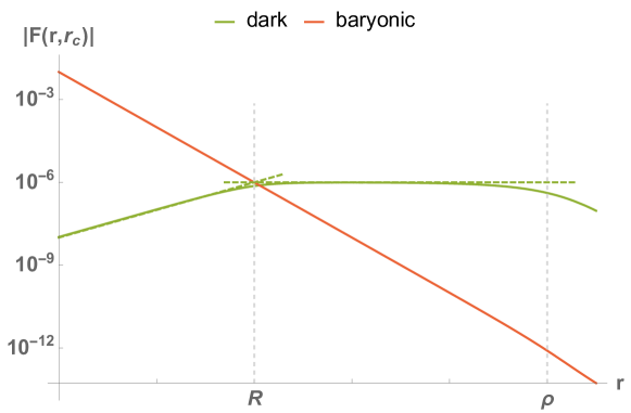
Figure 3: This log-log plot shows the force along the brane as a function of $r$ (in units of $R$). The ”dark” force (due to a point source with mass $M$ on the parallel brane), expressed in units of $\frac{GMm}{2R^{2}}$ (which is just $f$ from (LABEL:eq:f_numerical)), is plotted as the green solid curve. The green dashed curves are its asymptotes in regimes (III) and (II), given by $\frac{r}{r_{c}}$ and $\frac{1}{r_{c}}$. The red curve is the ”baryonic” force (due to a point source on the same brane), expressed in the same units. The ”baryonic” force is obtained numerically from (LABEL:eq:potential_baryonic), with $F_{\textnormal{B}}=-\frac{\partial}{\partial r}V_{\textnormal{B}}$ (see also footnote LABEL:fn:numerical_force). We did not plot the asymptote $\sim 1/r^{2}$, because in the regime $r\ll\rho$ it is indistinguishable from $F_{\textnormal{B}}$. The point mass, which gives rise to $F_{\textnormal{B}}$, is chosen such that both forces are of the same order at $r=R$. We chose the ratio $r_{c}/R=10^{6}$.

summarizes the above statement by comparing the ”baryonic” force to the ”dark” force (which is due to the point source on the parallel brane). We see that in this scenario, for $r\ll R$ (the interior of our galaxy), the usual baryonic force is much larger than the dark force. However, for $r\gtrsim R$, the constant dark force takes over.

It should be emphasized that the above distance independent force was derived for a point source at the 2nd brane. So it could be interesting to take an extended source and investigate how the asymptotic rotation-velocities would be impacted. It has been pointed out Oman2015 that there is a substantial diversity in the rotation curves in low surface brightness galaxies. This diversity might be explained by varying mass distributions on the parallel brane. Since in the present scenario only the parallel brane would contain this ”dark” matter distribution, it does not have to be weakly interacting, but could even form a highly localized density distribution.

Let us estimate, very crudely, the values of the involved length scales, such that the above outlined scenario can be valid. If we wish the distance independent force to be operational at $r\gtrsim 1\,$kpc, we should choose $R\sim 1\,$kpc. If we then want this regime to hold up to at least $r\gtrsim 10^{2}$ kpc, we should take

$$\rho\gtrsim 10^{2}\,\textnormal{kpc},$$ (18)

because for $r\gtrsim\rho$ the potential drops and the rotation-velocity would start to decrease. Since there is the constraint $r_{c}\gtrsim H_{0}^{-1}\sim 10^{6}\,$kpc from cosmological observations Deffayet2001, we actually need $\rho\gtrsim 10^{3}\,$kpc, which is significantly larger than the size of the galaxy. This constraint, however, does not necessarily imply that the constant force should extend to galaxy cluster scales, because our analysis shows that the constant force gets corrections as $r$ approaches $\rho$. For example, from Figure 3, we see that the force starts to deviate from its constant behavior for $r\gtrsim 10^{2}\,$kpc, if we take $\rho=10^{3}\,$kpc. A more detailed investigation is needed in order to establish the exact behavior of this new force at those large scales and to compare the results to predictions made by the usual cold dark matter scenario and to observations. We will postpone such an investigation to a future work.

Let us finally note that if the above scenario is valid, we have to ask the question, why is the mass on the parallel brane so tightly related to the mass in the ”baryonic” galaxy, as seen from (17). This question should then be addressed in the investigation of galaxy formation.

4 Kaluza-Klein decomposition

The Green’s function and the resulting potential energy can be derived in the Kaluza-Klein language. The advantage of this calculation is that we can gain more insight into the system and compare the results in both languages.

Let us shift the two branes, so that the system is symmetric around $y=0$:

$$S=\int\mbox{d}^{4}x\,\mathrm{d}y\,\left\{\frac{1}{2}\left(\partial_{A}\phi\right)^{2}+r_{c}\left[\delta\left(y+R/2\right)+\delta\left(y-R/2\right)\right]\frac{1}{2}\left(\partial_{\mu}\phi\right)^{2}+J(x^{\mu},y)\phi\right\}.$$ (19)

We can now expand the field $\phi$ in the following way:

$$\phi(x^{\mu},y)=\sum\limits_{\alpha=1}^{2}\int_{0}^{\infty}\mathrm{d}m\,\psi_{m,\alpha}(y)\phi_{m,\alpha}(x^{\mu}),$$

where $\phi_{m,\alpha}(x^{\mu})$ are the KK-modes and $\psi_{m,\alpha}(y)$ are the mode functions (or wave functions) constituting a complete basis of the $y$-space. We can make the Lagrangian in (19) diagonal in $\phi_{m,\alpha}(x^{\mu})$, if the mode functions satisfy the equation

$$\left\{\partial_{y}^{2}+m^{2}\left[1+r_{c}\delta\left(y+R/2\right)+r_{c}\delta\left(y-R/2\right)\right]\right\}\psi_{m,\alpha}(y)=0,$$ (20)

which implies the orthonormality condition

$$\int\mathrm{d}y\,\psi_{m,\alpha}(y)\psi_{m^{\prime},\alpha^{\prime}}(y)\left[1+r_{c}\delta\left(y+R/2\right)+r_{c}\delta\left(y-R/2\right)\right]=\delta(m-m^{\prime})\delta_{\alpha\alpha^{\prime}}.$$ (21)

Then, the action becomes c S=∫d^4 x   ∑_α ∫dm   { - 12ϕ_m,α(x^μ) [ □+ m^2 ] ϕ_m,α(x^μ) + ϕ_m,α(x^μ) J_m,α(x^μ) } ,
with $J_{m,\alpha}(x^{\mu})=\int\mathrm{d}y\,J(x^{\mu},y)\psi_{m,\alpha}(y)$. We can determine the basis $\{\psi_{m,\alpha}(y)\}$ by solving eq. (20). This is done in appendix LABEL:sec:mode_functions.

From the action (21) we derive the equation of motion

$$\left(\Box+m^{2}\right)\phi_{m,\alpha}(x^{\mu})=J_{m,\alpha}(x^{\mu}).$$ (22)

Since we are interested in the static source

$$J(x^{\mu},y)=g\left[\delta^{(3)}(\vec{x})\delta(y+R/2)+\delta^{(3)}(\vec{x}-\vec{r})\delta(y-R/2)\right],$$

we have

$$J_{m,\alpha}(x^{\mu})=g\left[\psi_{m,\alpha}(-R/2)\delta^{(3)}(\vec{x})+\psi_{m,\alpha}(R/2)\delta^{(3)}(\vec{x}-\vec{r})\right].$$ (23)

Then the solution of

$$\left(-\Delta+m^{2}\right)G_{m}(\vec{x}-\vec{x^{\prime}})=\delta^{(3)}(\vec{x}-\vec{x^{\prime}})$$ (24)

leads to the Green’s function

$$G_{m}(\vec{x}-\vec{x^{\prime}})=\int\frac{\mathrm{d}^{3}\vec{k}}{(2\pi)^{3}}\frac{\mathrm{e}^{\mathrm{i}\vec{k}(\vec{x}-\vec{x^{\prime}})}}{|\vec{k}|^{2}+m^{2}}=\frac{1}{4\pi r}\mathrm{e}^{-mr}.$$ (25)

Hence, the potential energy between the two sources is

$$V_{\text{KK}}(r,R)=-g^{2}\sum_{\alpha}\int_{0}^{\infty}\mathrm{d}m\,w_{m,\alpha}G_{m}(\vec{r}),$$ (26)

where we have defined the ”wave profile” rCl w_m,α &≡ ψ_m,α(-R/2) ψ_m,α(R/2)
=