Markovianity of the reference state, complete positivity of the reduced dynamics, and monotonicity of the relative entropy

Abstract

Consider the set $\mathcal{S}=\{\rho_{SE}\}$ of possible initial states of the system-environment, steered from a tripartite reference state $\omega_{RSE}$. Buscemi [F. Buscemi, Phys. Rev. Lett. 113, 140502 (2014)] showed that the reduced dynamics of the system, for each $\rho_{S}\in\mathrm{Tr}_{E}\mathcal{S}$, is always completely positive if and only if $\omega_{RSE}$ is a Markov state. There, during the proof, it has been assumed that the dimensions of the system and the environment can vary through the evolution. Here, we show that this assumption is necessary: we give an example for which, though $\omega_{RSE}$ is not a Markov state, the reduced dynamics of the system is completely positive, for any evolution of the system-environment during which the dimensions of the system and the environment remain unchanged. As our next result, we show that the result of Muller-Hermes and Reeb [A. Muller-Hermes and D. Reeb, Ann. Henri Poincare 18, 1777 (2017)], of monotonicity of the quantum relative entropy under positive maps, cannot be generalized to the Hermitian maps, even within their physical domains.

I Introduction

Consider a closed finite dimensional quantum system which evolves as

$$\rho\rightarrow\rho^{\prime}=\mathrm{Ad}_{U}(\rho)\equiv U\rho U^{\dagger},$$ (1)

where $\rho$ and $\rho^{\prime}$ are the initial and final states (density operators) of the system, respectively, and $U$ is a unitary operator. ($UU^{\dagger}=U^{\dagger}U=I$, where $I$ is the identity operator.)

In general, the system is not closed and interacts with its environment. We can consider the whole system-environment as a closed quantum system which evolves as Eq. (1). So the reduced state of the system after the evolution is given by

$$\rho_{S}^{\prime}=\mathrm{Tr}_{E}\circ\mathrm{Ad}_{U}(\rho_{SE})=\mathrm{Tr}_{E}\left(U\rho_{SE}U^{\dagger}\right),$$ (2)

where $\rho_{SE}$ is the initial state of the combined system-environment quantum system and $U$ acts on the whole Hilbert space of the system-environment.

There was a tendency to assume that the reduced dynamics of the system can always be written as a completely positive trace-preserving (CP) map; i.e. it can be written as

$$\rho_{S}^{\prime}=\sum_{i}E_{i}\,\rho_{S}\,E_{i}^{\dagger},\ \ \ \sum_{i}E_{i}^{\dagger}E_{i}=I_{S},$$ (3)

where $\rho_{S}=\mathrm{Tr}_{E}(\rho_{SE})$ is the initial state of the system. In addition, $E_{i}$ are linear operators and $I_{S}$ is the identity operator on the Hilbert space of the system $\mathcal{H}_{S}$ 1 .

But, in general, this is not the case. In fact, the CP-ness of the reduced dynamics has been proven only for some restricted sets of initial states of the system-environment 2 ; 3 ; 4 ; 5 ; 6 ; 7 ; 8 .

A remarkable result in this context is that given in 6 . Consider the set $\mathcal{S}$ of possible initial states of the system-environment, steered from a tripartite state $\omega_{RSE}$. There, it has been shown that, for all $\rho_{SE}\in\mathcal{S}$, the reduced dynamics of the system is CP, for arbitrary $U$, if and only if $\omega_{RSE}$ is a so-called Markov state.

The above result is important, not only because it includes all its previous results 7 , but also because it is, in fact, the most general possible result 9 , at least, within the framework of 10 . In the next section, we will review this result.

During the proof of the above result in 6 , it has been assumed that the dimensions of the Hilbert spaces of the system $\mathcal{H}_{S}$ and the environment $\mathcal{H}_{E}$ can vary during the system-environment evolution $U$, in general. In 11 , we have questioned whether this assumption can be relaxed or not. In Sec.  III, we show that this assumption is necessary for the result of 6 : we give an example, for which, though $\omega_{RSE}$ is not a Markov state, the reduced dynamics is CP, for any evolution $U$, which does not change $d_{S}$ and $d_{E}$, the dimensions of $\mathcal{H}_{S}$ and $\mathcal{H}_{E}$, respectively.

We give our next result, on monotonicity of quantum relative entropy, in Sec.  IV. The quantum relative entropy of the state $\rho$ to another state $\sigma$ is defined as

$$S(\rho||\sigma)=\mathrm{Tr}(\rho\mathrm{log}\rho)-\mathrm{Tr}(\rho\mathrm{log}\sigma),$$ (4)

if $\mathrm{supp}[\rho]\subseteq\mathrm{supp}[\sigma]$, otherwise it is defined to be $+\infty$ 1 . ($\mathrm{supp}[\eta]$, the support of the state $\eta$, is the subspace spanned by the eigenvectors of $\eta$ with nonzero eigenvalues.)

It was known that the relative entropy is monotone under CP maps $\Psi$ 1 ; 12 :

$$S(\rho||\sigma)\geq S(\Psi(\rho)||\Psi(\sigma)),$$ (5)

for arbitrary states $\rho$ and $\sigma$. Recently, the above result has been generalized to the case of positive trace-preserving maps, too 13 ; i.e., in Eq. (5), $\Psi$ can be a positive trace-preserving map. Positive maps are those which map any positive operator to a positive operator. If we consider positive maps as the most general physical time evolutions, then this result means that the relative entropy is monotone under any physical evolution.

But, in (14, ), it has been shown that any Hermitian trace-preserving map $\Phi$ is physical within its physical domain. By a Hermitian map, we mean a map which maps any Hermitian operator to a Hermitian operator. Therefore, $\Phi$ may maps a state to a non-positive operator. So, in (14, ), the physical domain of $\Phi$ is defined as the set of states which are mapped by $\Phi$ to density operators.

In Sec.  IV, using a theorem proven in 6 , we show that one can find physical evolutions, given by Hermitian trace-preserving maps $\Phi$, for which the relative entropy increases after the evolution. So, the result of 13 cannot be generalized to the Hermitian trace-preserving evolution, in general. In addition, we illustrate this result, using the example given in Sec.  III.

In the example considered in Sec.  IV, $d_{S}$ and $d_{E}$ vary through the evolution. In Sec.  V, we give another example in which the Hermitian non-positive evolution does not change $d_{S}$ and $d_{E}$, but the monotonicity of relative entropy is again violated. This shows that the variation of $d_{S}$ and $d_{E}$ is not necessary for the non-monotonicity of relative entropy, under Hermitian non-positive evolution.

Finally, in Sec.  VI, we end our paper, with a summary of our results.

II Reduced dynamics of an open quantum system

II.1 Reduced dynamics for a steered set

Consider the tripartite state $\omega_{RSE}$, on the Hilbert space of the reference-system-environment $\mathcal{H}_{R}\otimes\mathcal{H}_{S}\otimes\mathcal{H}_{E}$, where $\mathcal{H}_{R}$ is an ancillary Hilbert space. The set of steered states from performing measurements on the part $R$ of $\omega_{RSE}$ is 6

$$\mathcal{S}=\left\{\rho_{SE}=\frac{\mathrm{Tr}_{R}[(P_{R}\otimes I_{SE})\omega_{RSE}]}{\mathrm{Tr}[(P_{R}\otimes I_{SE})\omega_{RSE}]},P_{R}>0\right\},$$ (6)

where $P_{R}$ is arbitrary positive operator on $\mathcal{H}_{R}$ such that $\mathrm{Tr}[(P_{R}\otimes I_{SE})\omega_{RSE}]>0$ and $I_{SE}$ is the identity operator on $\mathcal{H}_{S}\otimes\mathcal{H}_{E}$. Note that, up to a positive factor, $P_{R}$ can be considered as an element of a POVM.

In Ref. 6 , it has been shown that the reduced dynamics of the system, for all $\rho_{S}\in\mathcal{S}_{S}\equiv\mathrm{Tr}_{E}\mathcal{S}$ and arbitrary $U$, is CP if and only if $\omega_{RSE}$ is a Markov state; i.e., if it can be written as 15

$$\omega_{RSE}=\mathrm{id}_{R}\otimes\Lambda_{S}^{CP}(\omega_{RS}),$$ (7)

where $\omega_{RS}=\mathrm{Tr}_{E}(\omega_{RSE})$, $\mathrm{id}_{R}$ is the identity map on $\mathcal{L}(\mathcal{H}_{R})$ and $\Lambda_{S}^{CP}\,:\mathcal{L}(\mathcal{H}_{S})\rightarrow\mathcal{L}(\mathcal{H}_{S}\otimes\mathcal{H}_{E})$ is a CP map. ($\mathcal{L}(\mathcal{H})$ is the space of linear operators on $\mathcal{H}$.)

When $\omega_{RSE}$ is a Markov state, then there exists a decomposition of the Hilbert space of the system $S$ as $\mathcal{H}_{S}=\bigoplus_{k}\mathcal{H}_{s_{k}}=\bigoplus_{k}\mathcal{H}_{s^{l}_{k}}\otimes\mathcal{H}_{s^{r}_{k}}$ such that

$$\omega_{RSE}=\bigoplus_{k}\lambda_{k}\>\omega_{Rs^{l}_{k}}\otimes\omega_{s^{r}_{k}E},$$ (8)

where $\{\lambda_{k}\}$ is a probability distribution ($\lambda_{k}\geq 0$, $\sum_{k}\lambda_{k}=1$), $\omega_{Rs^{l}_{k}}$ is a state on $\mathcal{H}_{R}\otimes\mathcal{H}_{s^{l}_{k}}$, and $\omega_{s^{r}_{k}E}$ is a state on $\mathcal{H}_{s^{r}_{k}}\otimes\mathcal{H}_{E}$ 15 .

Let us summarize the result of this subsection, for later reference 6 :

Theorem 1.

Assume that the set of possible initial states of the system-environment is given by $\mathcal{S}$, in Eq. (6), which is the steered set from a tripartite state $\omega_{RSE}$. The reduced dynamics of the system, in Eq. (2), is CP, for arbitrary $U$ and any $\rho_{SE}\in\mathcal{S}$, if and only if $\omega_{RSE}$ is a Markov state, as Eq. (8).

The following point is also worth noting. In this paper, when we say that the reduced dynamics is given by a CP map $\Psi$, we mean that there exists a CP extension of $\Psi$ to the whole $\mathcal{L}(\mathcal{H}_{S})$, as Eq. (3), such that the reduced dynamics of the system, for each $\rho_{S}\in\mathcal{S}_{S}$, is given by this CP map.

II.2 Reduced dynamics for an arbitrary set

A general framework for linear (Hermitian) reduced dynamics, when both the system and the environment are finite dimensional, has been introduced in 10 . In this paper, we will restrict ourselves to the case that there is a one to one correspondence between the system initial states $\rho_{S}$ and the system-environment initial states $\rho_{SE}$. So, in this subsection, we review the framework of 10 for this case.

Consider the set $\mathcal{S}=\{\rho_{SE}\}$ of possible initial states of the system-environment. Since, both the system and the environment are finite dimensional, a finite number $m$ of the members of $\mathcal{S}$, where the integer $m$ is $0<m\leq{(d_{S})}^{2}{(d_{E})}^{2}$, are linearly independent. Let us denote this linearly independent set as $\mathcal{S}^{\prime}=\{\rho_{SE}^{(1)},\rho_{SE}^{(2)},\ldots\ ,\rho_{SE}^{(m)}\}$. Therefore, any $\rho_{SE}\in\mathcal{S}$ can be written as $\rho_{SE}=\sum_{i=1}^{m}a_{i}\rho_{SE}^{(i)}$, where $a_{i}$ are real coefficients.

We restrict ourselves to the case that all $\rho_{S}^{(i)}=\mathrm{Tr}_{E}(\rho_{SE}^{(i)})\in\mathcal{S}^{\prime}_{S}\equiv\mathrm{Tr}_{E}\mathcal{S}^{\prime}$, $i=1,\dots,m\leq{(d_{S})}^{2}$, are also linearly independent. Therefore, there is a one to one correspondence between the members of $\mathcal{S}$ and the members of $\mathcal{S}_{S}=\mathrm{Tr}_{E}\mathcal{S}$. It is worth noting that when $\mathcal{S}$ is a steered set, as Eq. (6), from a Markov state $\omega_{RSE}$, as Eq. (7), then the above correspondence holds 9 .

The subspace $\mathcal{V}$ is defined as the subspace spanned by $\rho_{SE}^{(i)}\in\mathcal{S}^{\prime}$ 10 . Therefore, each $X\in\mathcal{V}$ can be expanded as $X=\sum_{i=1}^{m}c_{i}\rho_{SE}^{(i)}$, with complex coefficients $c_{i}$. In addition, for each $x=\mathrm{Tr}_{E}(X)\in\mathcal{V}_{S}\equiv\mathrm{Tr}_{E}\mathcal{V}$, we have $x=\sum_{i=1}^{m}c_{i}\rho_{S}^{(i)}$.

Let us denote the set of density operators in $\mathcal{L}(\mathcal{H}_{S}\otimes\mathcal{H}_{E})$ and $\mathcal{L}(\mathcal{H}_{S})$ by $\mathcal{D}_{SE}$ and $\mathcal{D}_{S}$, respectively. Note that $\mathcal{S}\subseteq\mathcal{V}\cap\mathcal{D}_{SE}$ and $\mathcal{S}_{S}\subseteq\mathcal{V}_{S}\cap\mathcal{D}_{S}$. So, that which we show for the whole $\mathcal{V}$ and $\mathcal{V}_{S}$ is also valid for their subsets $\mathcal{S}$ and $\mathcal{S}_{S}$, respectively.

Since all $\rho_{S}^{(i)}\in\mathcal{S}_{S}^{\prime}$ are linearly independent, as all $\rho_{SE}^{(i)}\in\mathcal{S}^{\prime}$, for each $x\in\mathcal{V}_{S}$, there is only one $X\in\mathcal{V}$ such that $\mathrm{Tr}_{E}(X)=x$. This allows us to define the linear assignment map $\Lambda_{S}$ as below. We define $\Lambda_{S}(\rho_{S}^{(i)})=\rho_{SE}^{(i)}$, $i=1,\ldots,m$. So, for any $x=\sum_{i=1}^{m}c_{i}\rho_{S}^{(i)}\in\mathcal{V}_{S}$, we have

$$\Lambda_{S}(x)=\sum_{i=1}^{m}c_{i}\Lambda_{S}(\rho_{S}^{(i)})=\sum_{i=1}^{m}c_{i}\rho_{SE}^{(i)}=X.$$ (9)

$\Lambda_{S}$ is a Hermitian map, by construction. It is defined on the whole $\mathcal{V}_{S}$, and even if $m<{(d_{S})}^{2}$, it can be simply extended to the whole $\mathcal{L}(\mathcal{H}_{S})$ 16 .

Although the assignment map $\Lambda_{S}$, in Eq. (9), is only a mathematical tool which acts as the reverse of $\mathrm{Tr}_{E}$, it has an important physical consequence. It allows us to assign to each $\rho_{S}\in\mathrm{Tr}_{E}(\mathcal{D}_{SE}\cap\mathcal{V})$ a $\rho_{SE}\in\mathcal{D}_{SE}\cap\mathcal{V}$ such that $\mathrm{Tr}_{E}(\rho_{SE})=\rho_{S}$. So, for any $\rho_{S}\in\mathrm{Tr}_{E}(\mathcal{D}_{SE}\cap\mathcal{V})$, and any unitary evolution $U$ of the whole system-environment, the reduced dynamics of the system, using Eqs. (2) and (9), is given by

$$\rho_{S}^{\prime}=\mathrm{Tr}_{E}\circ\mathrm{Ad}_{U}\circ\Lambda_{S}(\rho_{S})\equiv\Phi_{S}(\rho_{S}).$$ (10)

The unitary evolution $U$ and the partial trace $\mathrm{Tr}_{E}$ are CP maps 1 . We have seen that the assignment map $\Lambda_{S}$ is, in general, Hermitian. Therefore, the dynamical map $\Phi_{S}$ is, in general, a Hermitian map.

It is worth noting that for (the extension to the whole $\mathcal{L}(\mathcal{H}_{S})$ of) each linear trace-preserving Hermitian map, as $\Phi_{S}$, there exists an operator sum representation such that

$$\rho_{S}^{\prime}=\sum_{i}e_{i}\,\tilde{E_{i}}\,\rho_{S}\,\tilde{E_{i}}^{\dagger},\ \ \ \sum_{i}e_{i}\,\tilde{E_{i}}^{\dagger}\tilde{E_{i}}=I_{S},$$ (11)

where $\tilde{E_{i}}$ are linear operators on $\mathcal{H}_{S}$ and $e_{i}$ are real coefficients 17 ; 18 ; 10 . Only for the special case that all of the coefficients $e_{i}$ in Eq. (11) are positive, then we can define $E_{i}=\sqrt{e_{i}}\,\tilde{E_{i}}$ and so the reduced dynamics of the system is CP, as Eq. (3). (Also, for the Hermitian map $\Lambda_{S}$, there exists a similar operator sum representation, as Eq. (11), with linear operators $\tilde{E_{i}}:\mathcal{H}_{S}\rightarrow\mathcal{H}_{S}\otimes\mathcal{H}_{E}$.)

II.3 Reference state

In Ref. 9 , introducing the reference states $\omega_{RSE}$ and $\omega_{RS}=\mathrm{Tr}_{E}(\omega_{RSE})$, we have connected the results of 6 and 10 , reviewed in the two previous subsections. $\omega_{RS}$ is defined as 9

$$\omega_{RS}=\sum_{l=1}^{m}\frac{1}{m}|l_{R}\rangle\langle l_{R}|\otimes\rho_{S}^{(l)},$$ (12)

where $\rho_{S}^{(l)}\in\mathcal{S}^{\prime}_{S}$ and $\{|l_{R}\rangle\}$ is an orthonormal basis for the reference Hilbert space $\mathcal{H}_{R}$. In addition, the reference state $\omega_{RSE}$ is defined as 9

$$\omega_{RSE}=\mathrm{id}_{R}\otimes\Lambda_{S}(\omega_{RS})=\sum_{l=1}^{m}\frac{1}{m}|l_{R}\rangle\langle l_{R}|\otimes\rho_{SE}^{(l)},$$ (13)

where $\rho_{SE}^{(l)}\in\mathcal{S}^{\prime}$ is such that $\mathrm{Tr}_{E}(\rho_{SE}^{(l)})=\rho_{S}^{(l)}$.

We can construct subspaces $\mathcal{V}_{S}$ and $\mathcal{V}$ as the generalized steered sets, from $\omega_{RS}$ and $\omega_{RSE}$, respectively. We have 9

$$\mathcal{V}_{S}=\left\{\mathrm{Tr}_{R}[(A_{R}\otimes I_{S})\omega_{RS}]\right\},$$ (14)

and

$$\mathcal{V}=\left\{\mathrm{Tr}_{R}[(A_{R}\otimes I_{SE})\omega_{RSE}]\right\},$$ (15)

where $A_{R}$ are arbitrary linear operators in $\mathcal{L}(\mathcal{H}_{R})$.

When $\omega_{RSE}$, in Eq. (13), is a Markov state, as Eq. (7), i.e., when there exists a CP assignment map, then, using Eq. (10), the reduced dynamics $\Phi_{S}$ is, consequently, CP.

Comparing Eqs. (6) and (15), shows that, for the steered set $\mathcal{S}$ from the reference state $\omega_{RSE}$ in Eq. (13), we have $\mathcal{S}\subseteq\mathcal{D}_{SE}\cap\mathcal{V}$. So, when the reduced dynamics, for all $\rho_{SE}\in\mathcal{D}_{SE}\cap\mathcal{V}$, is CP, then, from Theorem 1, we conclude that $\omega_{RSE}$ is a Markov state, as Eq. (8).

In summary, we have 9 :

Theorem 2.

Consider the subspace $\mathcal{V}\subseteq\mathcal{L}(\mathcal{H}_{S}\otimes\mathcal{H}_{E})$, in Eq. (15). The reduced dynamics of the system, in Eq. (10), is CP, for arbitrary $U$ and any $\rho_{SE}\in\mathcal{D}_{SE}\cap\mathcal{V}$, if and only if the reference state $\omega_{RSE}$ in Eq. (13), is a Markov state, as Eq. (8).

III Markovianity of the reference state and complete positivity of the reduced dynamics

Theorem 2 is based on Theorem 1. In Ref. 6 , during the proof of Theorem 1, it has been assumed that, in general, the unitary time evolution $U:\mathcal{H}_{S}\otimes\mathcal{H}_{E}\rightarrow\mathcal{H}_{S}^{\prime}\otimes\mathcal{H}_{E}^{\prime}$ is such that the final Hilbert spaces of the system $\mathcal{H}_{S}^{\prime}$ and the environment $\mathcal{H}_{E}^{\prime}$ may differ from their initial ones, $\mathcal{H}_{S}$ and $\mathcal{H}_{E}$, respectively.

In Ref. 11 , we have questioned whether the above assumption can be relaxed or not. In other words, if the reduced dynamics, in Eq. (10), is CP, for arbitrary $U:\mathcal{H}_{S}\otimes\mathcal{H}_{E}\rightarrow\mathcal{H}_{S}\otimes\mathcal{H}_{E}$ and any $\rho_{SE}\in\mathcal{D}_{SE}\cap\mathcal{V}$, then whether we can conclude that the reference state $\omega_{RSE}$ in Eq. (13), is a Markov state, as Eq. (8), or not.

In this section, we consider an example, which is, in fact, example 4 of Ref. 10 , for which we see that, though the reference state is not a Markov state, the reduced dynamics is CP, for arbitrary $U:\mathcal{H}_{S}\otimes\mathcal{H}_{E}\rightarrow\mathcal{H}_{S}\otimes\mathcal{H}_{E}$ and any $\rho_{SE}\in\mathcal{D}_{SE}\cap\mathcal{V}$. Therefore, the assumption of variability of Hilbert spaces of the system and the environment, during the time evolution $U:\mathcal{H}_{S}\otimes\mathcal{H}_{E}\rightarrow\mathcal{H}_{S}^{\prime}\otimes\mathcal{H}_{E}^{\prime}$, is necessary, for validity of Theorems 1 and 2.

Assume that the set $\mathcal{S}^{\prime}$ is given by $\mathcal{S}^{\prime}=\{\rho,\sigma\}$, where $\rho=\frac{1}{d_{S}d_{E}}I_{SE}$ and $\sigma=|1_{S}\rangle\langle 1_{S}|\otimes|1_{E}\rangle\langle 1_{E}|$, $|1_{S}\rangle\in\mathcal{H}_{S}$ and $|1_{E}\rangle\in\mathcal{H}_{E}$. $\mathcal{V}$ is the subspace spanned by $\mathcal{S}^{\prime}$, and $\mathcal{V}_{S}$ is spanned by $\mathcal{S}^{\prime}_{S}=\{\tilde{\rho}=\frac{1}{d_{S}}I_{S},\tilde{\sigma}=|1_{S}\rangle\langle 1_{S}|\}$. $\mathcal{S}^{\prime}_{S}$ is a linearly independent set, as $\mathcal{S}^{\prime}$. So, there is a one to one correspondence between the members of $\mathcal{V}$ and $\mathcal{V}_{S}$. Therefore, from Sec. II.2, the reduced dynamics $\Phi_{S}$, in Eq. (10), is given by a Hermitian map, as Eq. (11), for arbitrary $U$ and any $\rho_{SE}\in\mathcal{D}_{SE}\cap\mathcal{V}$.

It can be shown simply that the assignment map $\Lambda_{S}$, in Eq. (9), is non-positive on $\mathcal{V}_{S}$ 10 : for $a\geq 0$ and $-\frac{a}{d_{S}}\leq b<-\frac{a}{d_{S}d_{E}}$, $x=a\tilde{\rho}+b\tilde{\sigma}\geq 0$, but $\Lambda_{S}(x)=a\rho+b\sigma\ngeqslant 0$. So, any extension of $\Lambda_{S}$, to the whole $\mathcal{L}(\mathcal{H}_{S})$, is also non-positive, at least, on $\mathcal{V}_{S}$. Therefore, we expect that the reference state $\omega_{RSE}$, in Eq. (13), is not a Markov state, as Eq. (8). In the following, we show this, explicitly. We have

$$\omega_{RSE}=\frac{1}{2}(|1_{R}1_{S}1_{E}\rangle\langle 1_{R}1_{S}1_{E}|+\frac{1}{d_{S}d_{E}}|2_{R}\rangle\langle 2_{R}|\otimes I_{SE}).$$ (16)

Note that $\langle 1_{R}1_{E}|\omega_{RSE}|1_{R}1_{E}\rangle=\frac{1}{2}|1_{S}\rangle\langle 1_{S}|$. If $\omega_{RSE}$ is a Markov state, then, from Eq. (8), we have

$$\langle 1_{R}1_{E}|\omega_{RSE}|1_{R}1_{E}\rangle=\bigoplus_{k}\lambda_{k}\>\eta_{s^{l}_{k}}\otimes\eta_{s^{r}_{k}}=\frac{1}{2}|1_{S}\rangle\langle 1_{S}|,$$ (17)

where $\eta_{s^{l}_{k}}$ and $\eta_{s^{r}_{k}}$ are positive operators on $\mathcal{H}_{s^{l}_{k}}$ and $\mathcal{H}_{s^{r}_{k}}$, respectively. Therefore

$$|1_{S}\rangle=|1_{s^{l}_{k_{0}}}\rangle|1_{s^{r}_{k_{0}}}\rangle,$$ (18)

where $|1_{s^{l}_{k_{0}}}\rangle\in\mathcal{H}_{s^{l}_{k_{0}}}$ and $|1_{s^{r}_{k_{0}}}\rangle\in\mathcal{H}_{s^{r}_{k_{0}}}$, for some $k_{0}$, and other $\eta_{s^{l}_{k}}$ and $\eta_{s^{r}_{k}}$, for $k\neq k_{0}$, are zero. Now, Eqs. (8) and (18) result that $\langle 1_{S}|\omega_{RSE}|1_{S}\rangle$ must be as $\eta_{R}\otimes\eta_{E}$, where $\eta_{R}$ and $\eta_{E}$ are positive operators on $\mathcal{H}_{R}$ and $\mathcal{H}_{E}$, respectively. But, from Eq. (16), it can be shown easily that $\langle 1_{S}|\omega_{RSE}|1_{S}\rangle$ cannot be written in a product form $\eta_{R}\otimes\eta_{E}$. Therefore, $\omega_{RSE}$, in Eq. (16), is not a Markov state.

Though $\omega_{RSE}$ is not a Markov state, it can be shown that the reduced dynamics, for arbitrary $U:\mathcal{H}_{S}\otimes\mathcal{H}_{E}\rightarrow\mathcal{H}_{S}\otimes\mathcal{H}_{E}$, is CP. Note that, if we do not extend $\Lambda_{S}$ to the whole $\mathcal{L}(\mathcal{H}_{S})$, the dynamical map $\Phi_{S}$, in Eq. (10), is a map on $\mathcal{V}_{S}$ . Now, by CP-ness of $\Phi_{S}$, we mean that there exists an extension of $\Phi_{S}$ to the whole $\mathcal{L}(\mathcal{H}_{S})$, as $\tilde{\Phi}_{S}$, such that $\tilde{\Phi}_{S}$ is a completely positive trace-preserving map, as Eq. (3).

A simple way of extending $\Phi_{S}$ is what is called zero extension 10 . First, we define the orthonormal projection $\mathcal{P}:\mathcal{L}(\mathcal{H}_{S})\rightarrow\mathcal{V}_{S}$ (according to the Hilbert-Schmidt inner product 1 ), as below. For any $A\in\mathcal{L}(\mathcal{H}_{S})$, we have

$$\mathcal{P}(A)=\sum_{i=1}^{2}\mathrm{Tr}(P_{i}A)P_{i},$$ (19)

where $P_{1}=|1_{S}\rangle\langle 1_{S}|$ and $P_{2}=\frac{1}{\sqrt{d_{S}-1}}\sum_{j=2}^{d_{S}}|j_{S}\rangle\langle j_{S}|$. $\{|j_{S}\rangle\}$ is an orthonormal basis for $\mathcal{H}_{S}$, including $|1_{S}\rangle$. $\mathcal{P}$ is CP, as Eq. (3), and, for each $x\in\mathcal{V}_{S}$, we have $\mathcal{P}(x)=x$. Now, the zero extension of $\Phi_{S}$ to the whole $\mathcal{L}(\mathcal{H}_{S})$ is

$$\tilde{\Phi}_{S}=\mathrm{Tr}_{E}\circ\mathrm{Ad}_{U}\circ\Lambda_{S}\circ\mathcal{P}.$$ (20)

From Eqs. (10) and (19), it is obvious that, for each $x\in\mathcal{V}_{S}$, we have $\tilde{\Phi}_{S}(x)=\Phi_{S}(x)$.

In Ref. 10 , by constructing the Choi matrix (operator) 19 , it has been shown that $\tilde{\Phi}_{S}$ is CP, for any $U:\mathcal{H}_{S}\otimes\mathcal{H}_{E}\rightarrow\mathcal{H}_{S}\otimes\mathcal{H}_{E}$. Consider the ket $|\xi\rangle=\sum_{i=1}^{d_{S}}|i_{R}\rangle|i_{S}\rangle\in\mathcal{H}_{R}\otimes\mathcal{H}_{S}$, which is, up to a normalization factor, the maximally entangled state. The Choi matrix, for the map $\tilde{\Phi}_{S}$, is 10

$$\mathrm{id}_{R}\otimes\tilde{\Phi}_{S}(|\xi\rangle\langle\xi|)=|1_{R}\rangle\langle 1_{R}|\otimes\mathrm{Tr}_{E}(U\sigma U^{\dagger})$$ (21)

$$+(I_{R}-|1_{R}\rangle\langle 1_{R}|)\otimes\frac{d_{S}\mathrm{Tr}_{E}(U\rho U^{\dagger})-\mathrm{Tr}_{E}(U\sigma U^{\dagger})}{d_{S}-1}.$$

When the final Hilbert spaces of the system and the environment are the same as their initial ones, i.e., for all $U:\mathcal{H}_{S}\otimes\mathcal{H}_{E}\rightarrow\mathcal{H}_{S}\otimes\mathcal{H}_{E}$, then $d_{S}\mathrm{Tr}_{E}(U\rho U^{\dagger})=I_{S}$. So, the Choi matrix is positive, since it is the summation of two positive operators. Therefore, $\tilde{\Phi}_{S}$ is CP.

According to Theorem 2, we expect, from the non-Markovianity of the reference state in Eq. (16), that there exists, at least, one unitary evolution $U:\mathcal{H}_{S}\otimes\mathcal{H}_{E}\rightarrow\mathcal{H}_{S}^{\prime}\otimes\mathcal{H}_{E}^{\prime}$ for which the reduced dynamics is non-CP. Assume $U_{0}$ is such that $\mathcal{H}_{S}^{\prime}=\mathcal{H}_{S}\otimes\mathcal{H}_{E}$, and $\mathcal{H}_{E}^{\prime}$ is a trivial one dimensional Hilbert space. (In fact, this $U_{0}$ is what has been used in Ref. 6 , during the proofs of Theorem 3, below, and, consequently, Theorem 1.) Then, the reduced dynamics of the system , for any $\rho_{S}\in\mathrm{Tr}_{E}(\mathcal{D}_{SE}\cap\mathcal{V})$, is given by

$$\rho_{S^{\prime}}^{\prime}=\Phi_{S}(\rho_{S})=\mathrm{Tr}_{E^{\prime}}\circ\mathrm{Ad}_{U_{0}}\circ\Lambda_{S}(\rho_{S})=\Lambda_{S}(\rho_{S}),$$ (22)

which is non-positive, since (any extension of) $\Lambda_{S}$ is non-positive.

Also, note that we have $d_{S}\mathrm{Tr}_{E^{\prime}}(U_{0}\rho U_{0}^{\dagger})=\frac{1}{d_{E}}I_{SE}$, and $\mathrm{Tr}_{E^{\prime}}(U_{0}\sigma U_{0}^{\dagger})=\sigma=|1_{S}\rangle\langle 1_{S}|\otimes|1_{E}\rangle\langle 1_{E}|$. So, the second term, on the right hand side of Eq. (21), is non-positive. Therefore, the zero extension $\tilde{\Phi}_{S}$, for $U_{0}$, is non-CP, too.

Using this fact that when there exists a positive assignment map $\Lambda_{S}$, then the reference state $\omega_{RSE}$, in Eq. (13), is a Markov state 16 , we can summarize the results of this section as below:

Proposition 1.

Consider the subspace $\mathcal{V}\subseteq\mathcal{L}(\mathcal{H}_{S}\otimes\mathcal{H}_{E})$, in Eq. (15). The reduced dynamics of the system, in Eq. (10), is Hermitian, for arbitrary $U$ and any $\rho_{S}\in\mathrm{Tr}_{E}(\mathcal{D}_{SE}\cap\mathcal{V})$. If the reference state $\omega_{RSE}$ in Eq. (13), is not a Markov state, as Eq. (8), then there exists, at least, one $U_{0}:\mathcal{H}_{S}\otimes\mathcal{H}_{E}\rightarrow\mathcal{H}_{S}^{\prime}\otimes\mathcal{H}_{E}^{\prime}$ for which the reduced dynamics is non-positive. But, the non-Markovianity of $\omega_{RSE}$ does not guarantee the non-CP-ness of the reduced dynamics, when the unitary evolution $U$ is such that $\mathcal{H}_{S}^{\prime}=\mathcal{H}_{S}$ and $\mathcal{H}_{E}^{\prime}=\mathcal{H}_{E}$.

Note that Proposition 1 includes a generalization of Theorems 1 and 2. Theorems 1 and 2 state that when $\omega_{RSE}$ is not a Markov state then there exists, at least, one $U_{0}$ such that the reduced dynamics is non-CP. But, Proposition 1 states that the non-Markovianity of $\omega_{RSE}$ leads to the non-positivity of the reduced dynamics, for, at least, one $U_{0}$, as Eq. (22), since the non-Markovianity of $\omega_{RSE}$ results in the non-positivity of the assignment map $\Lambda_{S}$ 16 .

IV Non-Markovianity of the reference state and monotonicity of the relative entropy

In Ref. 13 , it has been shown that the relative entropy, Eq. (4), is monotone under positive trace-preserving maps, as Eq. (5). As we have seen in Sec. II.2, the dynamical map $\Phi_{S}$, in Eq. (10), is, in general, a Hermitian trace-preserving map. Therefore, the question arises as to whether the relative entropy is monotone under Hermitian maps, too, or not.

In this section, we show that the result of Ref. 13 cannot be generalized to the Hermitian trace-preserving maps, in general. In other words, there exist physically admissible processes for which the relative entropy is not monotone.

First, note that, when the system and the environment undergo the unitary time evolution $U$, jointly, the reference state $\omega_{RSE}$, in Eq. (13), evolves as

$$\omega_{RSE}^{\prime}=\mathrm{id}_{R}\otimes\mathrm{Ad}_{U}(\omega_{RSE}).$$ (23)

This can be considered as an actual time evolution, for a tripartite closed quantum system of reference-system-environment, during which the reference remains unchanged.

From Eqs. (13) and (23), we have

$$\omega_{RSE}^{\prime}=\sum_{l=1}^{m}\frac{1}{m}|l_{R}\rangle\langle l_{R}|\otimes\rho_{SE}^{\prime(l)},$$ (24)

where $\rho_{SE}^{\prime(l)}=\mathrm{Ad}_{U}(\rho_{SE}^{(l)})$. Therefore, the evolution of $\omega_{RS}$, in Eq. (12), is given by

$$\omega_{RS}^{\prime}=\mathrm{Tr}_{E}(\omega_{RSE}^{\prime})=\sum_{l=1}^{m}\frac{1}{m}|l_{R}\rangle\langle l_{R}|\otimes\rho_{S}^{\prime(l)}$$ (25)

$$=\mathrm{id}_{R}\otimes\Phi_{S}(\omega_{RS})\equiv\Phi_{RS}(\omega_{RS}),$$

where $\rho_{S}^{\prime(l)}=\mathrm{Tr}_{E}(\rho_{SE}^{\prime(l)})$, and $\Phi_{S}$ is given in Eq. (10). Note that $\Phi_{S}$ is a Hermitian map, in general, and so is $\Phi_{RS}$.

In addition, from Eq. (25), we have $\omega_{R}^{\prime}=\mathrm{id}_{R}(\omega_{R})=\omega_{R}$ and $\omega_{S}^{\prime}=\Phi_{S}(\omega_{S})$, where $\omega_{R}=\mathrm{Tr}_{S}(\omega_{RS})$, $\omega_{R}^{\prime}=\mathrm{Tr}_{S}(\omega_{RS}^{\prime})$, $\omega_{S}=\mathrm{Tr}_{R}(\omega_{RS})$, and $\omega_{S}^{\prime}=\mathrm{Tr}_{R}(\omega_{RS}^{\prime})$. So, the evolution of the state $\sigma_{RS}=\omega_{R}\otimes\omega_{S}$ is also given by $\Phi_{RS}$; i.e., $\sigma_{RS}^{\prime}=\Phi_{RS}(\sigma_{RS})$. Equivalently, we can consider the tripartite state $\sigma_{RSE}=\omega_{R}\otimes\omega_{SE}$, where $\omega_{SE}=\mathrm{Tr}_{R}(\omega_{RSE})$, which evolves as Eq. (23): $\sigma_{RSE}^{\prime}=\mathrm{id}_{R}\otimes\mathrm{Ad}_{U}(\sigma_{RSE})$. Now, it can be shown easily that $\sigma_{RS}^{\prime}=\mathrm{Tr}_{E}(\sigma_{RSE}^{\prime})=\Phi_{RS}(\sigma_{RS})$.

Next, using Eq. (4), it can be shown that

$$S(\omega_{RS}||\sigma_{RS})=S(\omega_{RS}||\omega_{R}\otimes\omega_{S})$$ (26)

$$=S(\omega_{R})+S(\omega_{S})-S(\omega_{RS})$$

$$=I(R:S)_{\omega},$$

where $S(\rho)=-\mathrm{Tr}(\rho\mathrm{log}\rho)$ is the von Neumann entropy, and $I(R:S)_{\omega}$ is the mutual information, for the bipartite state $\omega_{RS}$ 1 . Similarly, we have $S(\omega_{RS}^{\prime}||\sigma_{RS}^{\prime})=I(R:S)_{\omega^{\prime}}$.

We want to verify whether the monotonicity relation, Eq. (5), is also valid for the Hermitian map $\Phi_{RS}$, within its physical domain, or not. We examine the monotonicity for the two states $\omega_{RS}$ and $\sigma_{RS}$. So, using Eq. (26), we want to verify whether

$$I(R:S)_{\omega}\geq I(R:S)_{\omega^{\prime}}.$$ (27)

The following theorem, proven in Ref. 6 , will be helpful:

Theorem 3.

Consider the tripartite state $\omega_{RSE}$, which evolves as Eq. (23). The inequality (27), for the bipartite state $\omega_{RS}$, holds, for arbitrary $U:\mathcal{H}_{S}\otimes\mathcal{H}_{E}\rightarrow\mathcal{H}_{S}^{\prime}\otimes\mathcal{H}_{E}^{\prime}$, if and only if $\omega_{RSE}$ is a Markov state, as Eq. (8).

Theorem 3 states that when $\omega_{RSE}$ is not a Markov state, e.g., Eq. (16), then there exists, at least, one $U$, for which the inequality (27) is violated. In other words, there exists, at least, one Hermitian map $\Phi_{RS}$, for which we have

$$S(\Phi_{RS}(\omega_{RS})||\Phi_{RS}(\sigma_{RS}))=I(R:S)_{\omega^{\prime}}$$ (28)

$$>I(R:S)_{\omega}=S(\omega_{RS}||\sigma_{RS}).$$

Therefore, the relative entropy is not monotone, under Hermitian maps, in general.

Let us illustrate Eq. (28), using the example considered in the previous section. Assuming that the system-environment evolution is given by $U_{0}$, using Eqs. (12), (13), and (22), we can easily show that

$$\Phi_{RS}(\omega_{RS})=\omega_{RSE},$$ (29)

$$\Phi_{RS}(\sigma_{RS})=\sigma_{RSE}=\omega_{R}\otimes\omega_{SE}.$$

So, as Eq. (26),

$$S(\Phi_{RS}(\omega_{RS})||\Phi_{RS}(\sigma_{RS}))=S(\omega_{RSE}||\omega_{R}\otimes\omega_{SE})$$ (30)

$$=S(\omega_{R})+S(\omega_{SE})-S(\omega_{RSE}).$$

Now, from Eqs. (26) and (30), we have

$$S(\Phi_{RS}(\omega_{RS})||\Phi_{RS}(\sigma_{RS}))-S(\omega_{RS}||\sigma_{RS})$$ (31)

$$=S(\omega_{RS})+S(\omega_{SE})-S(\omega_{RSE})-S(\omega_{S}).$$

The right hand side is always non-negative, using the strong subadditivity relation 1 . In fact, only when $\omega_{RSE}$ is a Markov state, as Eq. (8), the right hand side is zero; otherwise, it is greater that zero 15 . So, e.g., for $\omega_{RSE}$ in Eq. (16), the inequality (28) is satisfied, when the evolution of the reference-system-environment is given by $\mathrm{id}_{R}\otimes\mathrm{Ad}_{U_{0}}$. For this $\omega_{RSE}$, the right hand side of Eq. (31) is $0.2375$, when $d_{S}=d_{E}=2$.

V Non- monotonicity of the relative entropy for a Hermitian evolution which does not change initial Hilbert spaces

In the previous section, we have seen that the result of 13 , of monotonicity of relative entropy under positive maps, cannot be generalized to Hermitian maps, in general. The example, which we gave, illustrating this result, was for the case that the final Hilbert spaces $\mathcal{H}_{S}^{\prime}$ and $\mathcal{H}_{E}^{\prime}$ differ from their initial ones $\mathcal{H}_{S}$ and $\mathcal{H}_{E}$, respectively. In this section, we give another example, for which inequality (28) is satisfied, while $\mathcal{H}_{S}^{\prime}=\mathcal{H}_{S}$ and $\mathcal{H}_{E}^{\prime}=\mathcal{H}_{E}$, during the evolution.

We consider the example given in Ref. 20 , in which both the system and the environment are qubits. An arbitrary state of the system can be written as

$$\rho_{S}=\frac{1}{2}(I_{S}+\vec{\alpha}.\vec{\sigma}_{S}),$$ (32)

where $\vec{\sigma}_{S}=(\sigma^{(1)}_{S},\sigma^{(2)}_{S},\sigma^{(3)}_{S})$, $\sigma^{(i)}_{S}$ are the Pauli operators, and the Bloch vector $\vec{\alpha}=(\alpha^{(1)},\alpha^{(2)},\alpha^{(3)})$ is a real three dimensional vector such that $|\vec{\alpha}|\leq 1$ 1 .

Consider the following (linear trace-preserving) Hermitian assignment map $\Lambda_{S}$:

$$\Lambda_{S}(\sigma_{S}^{(i)})=\frac{1}{2}\sigma_{S}^{(i)}\otimes I_{E}\qquad(i=1,\,2,\,3),$$ (33)

$$\Lambda_{S}(I_{S})=\frac{1}{2}\left(I_{SE}+a\sum_{i=1}^{3}\sigma^{(i)}_{S}\otimes\sigma^{(i)}_{E}\right),$$

where $a$ is a fixed real constant. So,

$$\tau_{SE}\equiv\Lambda_{S}(\rho_{S})$$ (34)

$$=\frac{1}{4}\left(I_{SE}+\sum_{i=1}^{3}\alpha^{(i)}\sigma_{S}^{(i)}\otimes I_{E}+a\sum_{i=1}^{3}\sigma^{(i)}_{S}\otimes\sigma^{(i)}_{E}\right).$$

When $a\geq 0$, $\tau_{SE}$ is positive for $|\vec{\alpha}|\leq\sqrt{(1+a)(1-3a)}$, and when $a\leq 0$, $\tau_{SE}$ is positive for $|\vec{\alpha}|\leq(1+a)$ 20 ; 10 . Therefore, for $a\neq 0$, $\Lambda_{S}$ is a non-positive map.

The reference state $\omega_{RSE}$, for this example, is constructed in 9 :

$$\omega_{RSE}=\sum_{l=1}^{3}\frac{1}{16}|l_{R}\rangle\langle l_{R}|$$ (35)

$$\otimes\left(I_{SE}+\alpha^{(l)}\sigma_{S}^{(l)}\otimes I_{E}+a\sum_{i=1}^{3}\sigma^{(i)}_{S}\otimes\sigma^{(i)}_{E}\right)$$

$$+\frac{1}{16}|4_{R}\rangle\langle 4_{R}|\otimes(I_{SE}+a\sum_{i=1}^{3}\sigma^{(i)}_{S}\otimes\sigma^{(i)}_{E}),$$

where $\alpha^{(l)}$ are arbitrary real constants such that, for $a\geq 0$, $0<|\alpha^{(l)}|\leq\sqrt{(1+a)(1-3a)}$, and for $a\leq 0$, $0<|\alpha^{(l)}|\leq(1+a)$. From the non-positivity of the assignment map $\Lambda_{S}$, in Eq. (33), we expect that the reference state $\omega_{RSE}$ is non-Markovian. In 9 , it has been shown that $\omega_{RSE}$, in Eq. (35), is not a Markov state, as Eq. (8).

According to Theorem 2, the non-Markovianity of $\omega_{RSE}$ results in existence of, at least, one $U$, for which the reduced dynamics $\Phi_{S}$, in Eq. (10), is non-CP. In Ref. 20 , a class of unitary evolutions of the system-environment, as

$$U(\theta)=\left(\begin{matrix}1&0&0&0\\ 0&\mathrm{cos}\,\theta&\mathrm{sin}\,\theta&0\\ 0&-\mathrm{sin}\,\theta&\mathrm{cos}\,\theta&0\\ 0&0&0&1\end{matrix}\right),$$ (36)

has been introduced, where, for some values of $\theta$, the reduced dynamics of the system $\Phi_{S}(\theta)=\mathrm{Tr}_{E}\circ\mathrm{Ad}_{U(\theta)}\circ\Lambda_{S}$ is non-CP 20 ; 10 . The non-CP-ness of $\Phi_{S}(\theta)$ can be detected by calculating the eigenvalues of the Choi matrix of it. For this example, the Choi matrix is given explicitly in 10 . When, at least, one of the eigenvalues of the Choi matrix is negative, then $\Phi_{S}(\theta)$ is non-CP. For this example, the eigenvalues of the Choi matrix can be calculated analytically. In Fig.1.b, three of the eigenvalues of the Choi matrix, which are negative, for some values of $\theta$, are plotted, for $a=-0.8$. (The fourth one is always positive.)

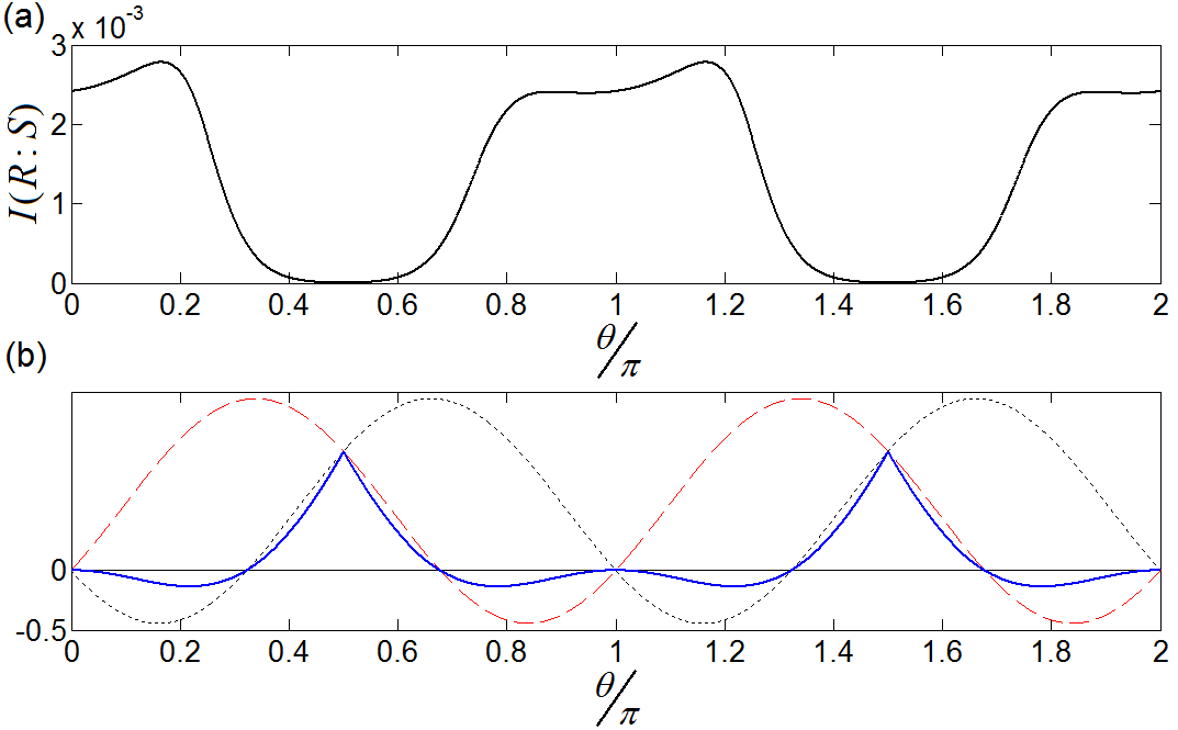
Figure 1: (a) Mutual information $I(R:S)_{\omega(\theta)}$, as a function of $\theta$, for $a=-0.8$, $\alpha^{(1)}=0.15b$, $\alpha^{(2)}=0.25b$, and $\alpha^{(3)}=-0.6b$, where $b=1+a$, in Eq. (35). (b) Three of the eigenvalues of the Choi matrix, which are negative, for some values of $\theta$, for $a=-0.8$.

Non-CP-ness of $\Phi_{S}(\theta)$ results in non-positivity of $\Phi_{RS}(\theta)=\mathrm{id}_{R}\otimes\Phi_{S}(\theta)$, since $d_{R}=4>2=d_{S}$. From Eq. (25), we have $\omega_{RS}(\theta)=\Phi_{RS}(\theta)[\omega_{RS}]$, where $\omega_{RS}=\mathrm{Tr}_{E}(\omega_{RSE})$, and $\omega_{RSE}$ is given in Eq. (35). Fortunately, for this example, the eigenvalues of $\omega_{RS}(\theta)$ and $\omega_{S}(\theta)=\mathrm{Tr}_{R}[\omega_{RS}(\theta)]$ can be calculated analytically. Therefore, from Eq. (26), $I(R:S)_{\omega(\theta)}$, where $\omega(\theta)=\omega_{RS}(\theta)$ can, also, be calculated analytically. In Fig.1.a, the mutual information $I(R:S)_{\omega(\theta)}$ is plotted as the function of $\theta$. Fig. 1.a shows that $I(R:S)_{\omega(\theta)}$ exceeds its initial value, for some values of $\theta$. So, for these values of $\theta$, the inequality (28) is satisfied. Note that the unitary evolution $U(\theta)$, in Eq. (36), does not change $\mathcal{H}_{S}$ and $\mathcal{H}_{E}$.

Let us summarize the result of the two last sections:

Proposition 2.

The result of 13 , of monotonicity of the relative entropy under positive trace-preserving maps, cannot be generalized to the Hermitian trace-preserving non-positive maps, within their physical domains, in general. Inequality (28) can be satisfied, both when $\mathcal{H}_{S}$ and $\mathcal{H}_{E}$ vary, during the non-positive evolution $\Phi_{RS}=\mathrm{id}_{R}\otimes\Phi_{S}$, and when they do not vary.

To achieve the above result, first, we have considered the time evolution of reference-system-environment as Eq. (23), which allows us to use Theorem 3. Second, we have considered the two appropriate states $\omega_{RS}$ and $\sigma_{RS}$, for which we can write Eq. (26), both before and after the evolution $\Phi_{RS}=\mathrm{id}_{R}\otimes\Phi_{S}$. Therefore, we could write the monotonicity relation, Eq. (5), as the inequality (27), which, from Theorem 3, we know is violated for a non-Markovian $\omega_{RSE}$, for, at least, one $U$.

Note that $\sigma_{S}=\mathrm{Tr}_{R}(\sigma_{RS})=\omega_{S}$ and, so, $\sigma_{S}^{\prime}=\Phi_{S}(\sigma_{S})=\omega_{S}^{\prime}$. Therefore, for the two equal states $\omega_{S}$ and $\sigma_{S}$ (and the evolution $\Phi_{S}$) the monotonicity relation, Eq. (5), is, trivially, satisfied. But, as we have seen, the evolution $\Phi_{RS}=\mathrm{id}_{R}\otimes\Phi_{S}$ can lead to the violation of the inequality (5), for the two states $\omega_{RS}$ and $\sigma_{RS}$.

VI Summary

In Ref. 9 , we have introduced the reference states $\omega_{RSE}$, Eq. (13), and $\omega_{RS}$, Eq. (12). There, we have used them to connect the results of 6 and 10 , as reviewed in Sec. II. In this paper, we have given two other results, using these reference states.

First, in Sec. III, giving an explicit example, we have shown that, even when $\omega_{RSE}$ is not a Markov state, as Eq. (8), the reduced dynamics of the system can be CP, for arbitrary system-environment unitary evolution $U$, which does not change $d_{S}$ and $d_{E}$.

This shows that the assumption of variability of Hilbert spaces of the system and the environment, during the time evolution $U:\mathcal{H}_{S}\otimes\mathcal{H}_{E}\rightarrow\mathcal{H}_{S}^{\prime}\otimes\mathcal{H}_{E}^{\prime}$, is necessary, for validity of Theorems 1 and 2.

Second, in Sec. IV, considering the time evolution of the reference states $\omega_{RSE}$ and $\omega_{RS}$, and using Theorem 3, proven in 6 , we have shown that, when $\omega_{RSE}$ is not a Markov state, then there exists, at least, one Hermitian non-positive map $\Phi_{RS}=\mathrm{id}_{R}\otimes\Phi_{S}$, for which the inequality (28) is satisfied. Note that $\omega_{RS}$ and $\sigma_{RS}$, in Eq. (28), are in the physical domain of $\Phi_{RS}$. Therefore, the relative entropy is not monotone, under Hermitian non-positive maps, even within their physical domains, in general.

When $\omega_{RSE}$ is not a Markov state, any possible assignment map $\Lambda_{S}$ is non-positive 16 . So, choosing $\Phi_{S}=\Lambda_{S}$, as Eq. (22), results in a non-positive $\Phi_{RS}$. In Sec. IV, we have seen that, at least, for this $\Phi_{RS}$, inequality (28) is satisfied.

In addition to the above example, which includes changes in $d_{S}$ and $d_{E}$ after the evolution, in Sec. V, we have given another example, for which inequality (28) is satisfied, while $\mathcal{H}_{S}$ and $\mathcal{H}_{E}$ remain unchanged, during the evolution.

References

- (1) M. A. Nielsen and I. L. Chuang, Quantum Computation and Quantum Information (Cambridge University Press, Cambridge, 2000).
- (2) C. A. Rodríguez-Rosario, K. Modi, A.-m. Kuah, A. Shaji and E. C. G. Sudarshan, Completely positive maps and classical correlations, J. Phys. A: Math. Theor. 41, 205301 (2008).
- (3) A. Shabani and D. A. Lidar, Vanishing quantum discord is necessary and sufficient for completely positive maps, Phys. Rev. Lett. 102, 100402 (2009); Phys. Rev. Lett. 116, 049901 (2016).
- (4) L. Liu and D. M. Tong, Completely positive maps within the framework of direct-sum decomposition of state space, Phys. Rev. A 90, 012305 (2014).
- (5) A. Brodutch, A. Datta, K. Modi, A. Rivas and C. A. Rodríguez-Rosario, Vanishing quantum discord is not necessary for completely positive maps, Phys. Rev. A 87, 042301 (2013).
- (6) F. Buscemi, Complete positivity, Markovianity, and the quantum data-processing inequality, in the presence of initial system-environment correlations, Phys. Rev. Lett. 113, 140502 (2014).
- (7) X.-M. Lu, Structure of correlated initial states that guarantee completely positive reduced dynamics, Phys. Rev. A 93, 042332 (2016).
- (8) I. Sargolzahi and S. Y. Mirafzali, When the assignment map is completely positive, Open Sys. Info. Dyn. 25, 1850012 (2018).
- (9) I. Sargolzahi, Reference state for arbitrary U-consistent subspace, J. Phys. A: Math. Theor. 51, 315301 (2018).
- (10) J. M. Dominy, A. Shabani and D. A. Lidar, A general framework for complete positivity, Quantum Inf. Process. 15, 465 (2016).
- (11) I. Sargolzahi and S. Y. Mirafzali, Structure of states for which each localized dynamics reduces to a localized subdynamics, Int. J. Quantum Inf. 15, 1750043 (2017).
- (12) G. Lindblad, Completely positive maps and entropy inequalities, Commun. math. Phys. 40, 147 (1975).
- (13) A. Muller-Hermes and D. Reeb, Monotonicity of the quantum relative entropy under positive maps, Ann. Henri Poincare 18, 1777 (2017).
- (14) J. M. Dominy and D. A. Lidar, Beyond complete positivity, Quantum Inf. Process. 15, 1349 (2016).
- (15) P. Hayden, R. Jozsa, D. Petz and A. Winter, Structure of states which satisfy strong subadditivity of quantum entropy with equality, Commun. Math. Phys. 246, 359 (2004).
- (16) I. Sargolzahi, Positivity of the assignment map implies complete positivity of the reduced dynamics, arXiv:1906.11502 (2019).
- (17) E. C. G. Sudarshan, P. M. Mathews and J. Rau, Stochastic dynamics of quantum-mechanical systems, Phys. Rev. 121, 920 (1961).
- (18) T. F. Jordan, A. Shaji and E. C. G. Sudarshan, Dynamics of initially entangled open quantum systems, Phys. Rev. A 70, 052110 (2004).
- (19) M.-D. Choi, Completely positive linear maps on complex matrices, Linear Alg. Appl. 10, 285 (1975).
- (20) H. A. Carteret, D. R. Terno and K. Zyczkowski, Dynamics beyond completely positive maps: Some properties and applications, Phys. Rev. A 77, 042113 (2008).