Lindblad dynamics of the damped and forced quantum harmonic oscillator

Abstract

The quantum dynamics of a damped and forced harmonic oscillator is investigated in terms of a Lindblad master equation. Elementary algebraic techniques are employed allowing for example to analyze the long time behavior, i.e. the quantum limit cycle. The time evolution of various expectation values is obtained in closed form as well as the entropy and the Husimi phase space distribution. We also discuss the related description in terms of a non-Hermitian Hamiltonian.

1 Introduction

In classical mechanics, the damped and driven harmonic oscillator is one of the paradigmatic systems discussed in elementary physics lectures, modeling for example a mass attached to a linear spring in the gravitational field. The dynamics is linear and allows a closed form solution, which then serves as a basic model for analyzing more general and, of course, much more demanding general dynamical systems. The harmonic oscillator also constitutes a basic building block in elementary quantum mechanics, however almost exclusively in context with Hermitian dynamics, which is also in most cases restricted to systems with no explicit time-dependence, though also a time-depended force can be treated quite elementary, as for instance in the book by Louisell [1, sect. 3.11]. The damped quantum harmonic oscillator is, however, addressed very rarely in elementary texts. Exceptions are, e.g., the recent paper by Fujii [2] describing in much detail the dissipative quantum dynamics in terms of the Lindblad master equations, however for the force-free case. This system is also described in the article [3] as well as in lecture notes by Englert and Morigi [4], where also a quantum-optical system with periodic driving is studied, describing a decaying photon field excited by periodic kicking.

An elementary study of the Lindblad dynamics of a forced harmonic oscillator seems to be missing, however, and here we will try to fill this gap. We follow the analysis in [2], describing briefly these results for the non-driven system in section 3. In this case the general solution can be constructed and the density operator is expressed in closed form. This is, however, not fully achieved in the present analysis of the driven oscillator in section 4. We will derive a special class of solutions using similar techniques as in our previous study of a related model [5]. Nevertheless we will be able to describe some important features of the dynamics, as for example the density operator for the quantum limit cycle. Section 5 is devoted to a related description of quantum damping in terms of non-Hermitian Hamiltonians, in the present case a harmonic oscillator with a complex frequency. For convenience of the reader we begin with a brief repetition of the well-known classical dynamics. We will use units with $\hbar=1$ throughout.

2 The classical oscillator

Let us briefly recall the damped and driven harmonic oscillator in classical mechanics. The equation of motion

$$\ddot{x}+2\gamma\dot{x}+\omega_{0}^{2}x=\tilde{f}(t)$$ (1)

models a harmonic oscillator with frequency $\omega_{0}$ under a time-dependent force $\tilde{f}(t)$, which will be assumed to be harmonic,

$$\tilde{f}(t)=\tilde{f}_{0}\cos\Omega t\,,$$ (2)

in the following. The interaction with an environment is modeled by the term $2\gamma\dot{x}$ where the constant $\gamma>0$ describes the friction. For a free motion with vanishing force the general solution is given by

$$x(t)=x_{+}{\rm e}^{+{\rm i}\omega t-\gamma t}+x_{-}{\rm e}^{-{\rm i}\omega t-\gamma t}\,,$$ (3)

where the constants $x_{+}$ and $x_{-}$ are determined by the initial conditions. The frequency

$$\omega=\sqrt{\omega_{0}^{2}-\gamma^{2}}$$ (4)

is real valued in the underdamped case, $\gamma<\omega_{0}$, resulting in an oscillatory motion, whereas $\omega$ is imaginary for strong damping, $\gamma>\omega_{0}$, and both terms in (3) are exponentially decaying. In any case, the free solution finally approaches $x=0$. For a harmonic force (2) one can construct a special solution, the limit cycle

$$x^{\rm(\ell c)}(t)=A\cos(\Omega t+\phi)\,,$$ (5)

where the motion follows the external force, shifted by a phase

$$\phi=-\arctan\frac{2\gamma\Omega}{\omega_{0}^{2}-\Omega^{2}}$$ (6)

with an amplitude

$$A=\frac{\tilde{f}_{0}}{\sqrt{(\omega_{0}^{2}-\Omega^{2})^{2}+(2\gamma\Omega)^{2}}}.$$ (7)

The general solution is given by a sum of (3) and (5). Then for all initial conditions the solution $x(t)$ converges to the limit cycle (5). As a function of the external frequency $\Omega$, the limit cycle shows the celebrated resonance behavior, where the amplitude $A$ shows a maximum of height $A_{R}=\tilde{f}_{0}/(2\gamma\sqrt{\omega_{0}^{2}-\gamma^{2}})$ at the resonance frequency $\Omega_{R}=\sqrt{\omega_{0}^{2}-2\gamma^{2}}$ for $\omega_{0}^{2}>\gamma^{2}$ and the phase shift $\phi$ changes from $\phi=0$ for $\Omega=0$ to $\phi=-\pi$ for large $\Omega$. If we identify $\dot{x}$ with the momentum $p$ (assuming unit mass) the limit cycle appears in phase space as an ellipse, namely

$$p^{2}/\Omega^{2}+x^{2}=A^{2}\,.$$ (8)

3 The Lindblad master equation

The quantum dynamics of our system is described by the Lindblad master equation

$$\frac{{\rm d}\hat{\rho}}{{\rm d}t}={\mathcal{L}}\hat{\rho}=-{\rm i}\,\big{[}\hat{H},\hat{\rho}\,\big{]}$$

$$\qquad+\frac{\mu}{2}\,\big{(}2\hat{a}\hat{\rho}\hat{a}^{\dagger}-\hat{a}^{\dagger}\hat{a}\hat{\rho}-\hat{\rho}\hat{a}^{\dagger}\hat{a}\big{)}+\frac{\nu}{2}\,\big{(}2\hat{a}^{\dagger}\hat{\rho}\hat{a}-\hat{a}\hat{a}^{\dagger}\hat{\rho}-\hat{\rho}\hat{a}\hat{a}^{\dagger}\big{)},$$ (9)

where the $\mu$- and $\nu$-terms represent (homogeneous) loss and (inhomogeneous) pumping of particles, respectively. Note that often these coefficients are written as $\mu=\gamma_{0}(1+\overline{n})$ and $\nu=\gamma_{0}\,\overline{n}$, where $\overline{n}=\nu/(\mu-\nu)$ is the thermal population of the environment. In the following it will be convenient to rewrite the damping coefficients as

$$\mu=\gamma^{\prime}+\gamma\ ,\quad\nu=\gamma^{\prime}-\gamma\,,$$ (10)

where $\gamma^{\prime}$ and $\gamma$ are denoted as diffusion and dissipation constants [6]. We will assume $\mu>\nu\geq 0$ so that $\gamma^{\prime}=(\mu+\nu)/2$ and $\gamma=(\mu-\nu)/2$ are positive. A motivation and some applications of this evolution equation can be found in [4] or [7], where it is shown that this evolution equation can, for example, describe the damping of an electromagnetic field mode inside a cavity. The modes outside the cavity in a thermal reservoir cause a damping with rate $\gamma$.

It may be recalled that the density operator $\hat{\rho}(t)$ is a positive operator with unit trace and the Lindblad evolution conserves the trace and the positivity of $\hat{\rho}$. The expectation value of an observable $\hat{A}$ is given by

$$\langle\hat{A}\rangle_{t}={\rm\,trace\,}(\hat{A}\hat{\rho}(t))\,,$$ (11)

where we have assumed that $\hat{A}$ is not explicitly time-dependent. If $\hat{H}$ is Hermitian, we have

$$\langle\hat{A}^{\dagger}\rangle_{t}=\langle\hat{A}\rangle^{*}_{t}\,.$$ (12)

The Hamiltonian of the forced harmonic oscillator is

$$\hat{H}=\omega\big{(}\hat{a}^{\dagger}\hat{a}+1/2\big{)}-f^{*}(t)\,\hat{a}^{\dagger}-f(t)\,\hat{a}$$ (13)

with time-independent real $\omega$, where $\hat{a}^{\dagger}$ and $\hat{a}$ are the familiar bosonic creation and destruction operators with commutator $|\hat{a},\hat{a}^{\dagger}]=1$. We will also use the number operator $\hat{n}=\hat{a}^{\dagger}\hat{a}$, whose eigenvalues $n=0,\,1,\,\ldots$ are the number of oscillator quanta, sometimes also denoted as the number of photons or simply particles. This Hamiltonian models, for example, the coherent excitation of the cavity field by a monochromatic laser.

The Hamiltonian is Hermitian and can be rewritten as

$$\hat{H}=\omega\big{(}\hat{a}^{\dagger}\hat{a}+1/2\big{)}-\tilde{f}(t)\,\hat{x}$$ (14)

for a real valued force, using

$$\hat{x}=(\hat{a}^{\dagger}+\hat{a})/\sqrt{2\omega},\quad\hat{p}={\rm i}(\hat{a}^{\dagger}-\hat{a})\sqrt{\omega/2}\quad\textrm{and}\quad\tilde{f}(t)=\sqrt{2\omega}\,f(t)\,.$$ (15)

In the following we will consider some special cases in more detail, namely a force-free system, $f(t)=0$, which is time-independent and allows the construction of a general analytical solution $\hat{\rho}(t)$, and a harmonic driving $f(t)=f_{0}\,\cos\Omega t$ with real valued amplitude $f_{0}$. Here a closed form solution can be derived for a special set of initial distributions.

Without the forcing term, the density $\hat{\rho}(t)$ approaches for $\nu>0$ in the long time limit the steady state distribution [4]

$$\hat{\rho}^{\rm(ss)}=(1-\nu/\mu)\,{\rm e}^{\,\ln(\nu/\mu)\,\hat{n}}$$ (16)

and the mean value $\langle\hat{n}\rangle$ is equal to $\overline{n}=\nu/(\mu-\nu)=\nu/2\gamma$, which agrees with the mean number of photons in the environment if the system models a photon field in a cavity. For $\nu=0$, where we have no gain, the steady state distribution is given by the oscillator ground state $\hat{\rho}^{\rm(ss)}=|0\rangle\langle 0|$. In the following we will be interested in the Lindblad dynamics of a forced harmonic oscillator, where the force is time-dependent with emphasis on a harmonic driving.

The Lindblad equation (9) can, of course, be solved numerically (a simple Matlab program can be found in [8]), but the dynamics shows various features, which are not directly obvious and a closed form exact solution is in many cases preferable, in particular for such a quite elementary system. In the following we will discuss this in some detail. A general solution describing the density operator $\hat{\rho}(t)$ for any given $\hat{\rho}_{0}$ has been presented recently by Fujii [2] for the non-driven case and some of these results will be given below. Solutions, however, can also be found for a driven system, as for instance for the expectation values of position, momentum and energy, or for a special class of density operators as shown in the following sections.

3.1 The force-free oscillator

For a free evolution, $f(t)=0$, the Hamiltonian is time-independent, which considerably simplifies the analysis. A full solution has been presented recently by Fujii [2] based on previous work [9, 10]. Here the dynamics of the density operator is mapped on a vector evolution using the Kronecker product (see also the book by Steeb and Hardy [11] as well as [12]). This derivation is heavily based on techniques from operator algebra and here we only state the final result obtained in [2], namely

$$\hat{\rho}(t) = \frac{{\rm e}^{\gamma t}}{F(t)}\sum_{j=0}^{\infty}\frac{G(t)^{j}}{j!}\hat{a}^{\dagger\,j}\,{\rm e}^{\{-{\rm i}\omega t-\ln F(t)\}\hat{n}}\times$$ (17)

$$\qquad\qquad\Big{\{}\sum_{k=0}^{\infty}\frac{E(t)^{k}}{k!}\hat{a}^{k}\hat{\rho}_{0}\,\hat{a}^{\dagger k}\Big{\}}\,{\rm e}^{\{+{\rm i}\omega t-\ln F(t)\}\hat{n}}\,\hat{a}^{j}\,,$$

where the three functions $E(t)$, $F(t)$ and $G(t)$ are solutions of some first order differential equations with $F(0)=1$ and $E(0)=G(0)=0$. Let us note, for example, that $G(t)$ solves the Riccati equation

$$\dot{}u+(\mu+\nu)u-\mu u^{2}=\nu\,,$$ (18)

for an initial condition $u(0)=0$. As shown in [2] these functions are given by

$$F(t) = \cosh\gamma t+(\gamma^{\prime}/\gamma)\sinh\gamma t$$ (19)

$$E(t) = \frac{\mu}{\gamma F(t)}\sinh\gamma t\ ,\quad G(t)=\frac{\nu}{\gamma F(t)}\sinh\gamma t\,.$$ (20)

The general solution (17) simplifies for special cases (see [2] for details):
$(\bullet)$ For $\nu=0$ one obtains

$$\hat{\rho}(t)={\rm e}^{-(\mu/2+{\rm i}\omega)t\,\hat{n}}\Big{\{}\sum_{k=0}^{\infty}\frac{E(t)^{k}}{k!}\hat{a}^{k}\hat{\rho}_{0}\,\hat{a}^{\dagger k}\Big{\}}{\rm e}^{-(\mu/2-{\rm i}\omega)t\,\hat{n}}\,.$$ (21)

$(\bullet)$ If $\nu\neq 0$ and the initial state is the oscillator ground state $\hat{\rho}_{0}=|0\rangle\langle 0|$, we have

$$\hat{\rho}(t)=(1-G(t))\,{\rm e}^{\,\ln G(t)\,\hat{n}}$$ (22)

and the mean value of $\hat{n}$ is given by

$$\langle\hat{n}\rangle_{t}={\rm\,trace\,}(\hat{n}\hat{\rho}(t))=\frac{\nu}{2\gamma}\Big{(}1-{\rm e}^{-2\gamma t}\Big{)}\,.$$ (23)

Here the system is for all times in a thermal state, i.e. a canonical distribution. In the long time limit we clearly see with $G(t)\rightarrow\nu/\mu$ the convergence toward the steady state distribution (16).

$(\bullet)$ For $\nu\neq 0$ and a coherent initial state $\hat{\rho}_{0}=|\alpha_{0}\rangle\langle\alpha_{0}|$ the solution is given by

$$\hat{\rho}(t)={\rm e}^{c(t)-\log G(t)\big{(}\alpha(t)\hat{a}^{\dagger}+\alpha^{*}(t)\hat{a}-\hat{n}\big{)}}$$ (24)

with

$$c(t)=|\alpha(t)|^{2}\log G(t)+\log(1-G(t))\ ,\quad\alpha(t)=\alpha_{0}{\rm e}^{-(\gamma+{\rm i}\omega)t}\,.$$ (25)

(compare eq. (4.3) in [2]), or, written in product form using the disentangling relation given in eq. (56) below,

$$\hat{\rho}(t)={\rm e}^{\tilde{c}(t)}{\rm e}^{(1-G(t))\alpha(t)\hat{a}^{\dagger}}{\rm e}^{\log G(t)\hat{n}}{\rm e}^{(1-G(t))\alpha^{*}(t)\hat{a}}$$ (26)

with

$$\tilde{c}(t)=\log(1-G(t))-|\alpha(t)|^{2}(1-G(t))\,.$$ (27)

$(\bullet)$ Finally, for $\hat{\rho}_{0}=|\alpha_{0}\rangle\langle\alpha_{0}|$ and $\nu=0$, we find from (21)

$$\hat{\rho}(t) = {\rm e}^{(1-{\rm e}^{-\mu t})|\alpha_{0}|^{2}}\,{\rm e}^{-(\mu/2+{\rm i}\omega)t\,\hat{n}}\,|\alpha_{0}\rangle\langle\alpha_{0}|\,{\rm e}^{-(\mu/2-{\rm i}\omega)t\,\hat{n}}$$ (28)

$$= |\alpha(t)\rangle\langle\alpha(t)|\quad\textrm{with}\quad\alpha(t)=\alpha_{0}\,{\rm e}^{-(\mu/2+{\rm i}\omega)t}$$

(compare eq. (127) in appendix A), i.e. the system remains in a coherent state for all times and the mean values of $\hat{a}$ and $\hat{n}$ decay as

$$\langle\hat{a}\rangle_{t}=\alpha(t)\ ,\quad\langle\hat{n}\rangle_{t}=|\alpha(t)|^{2}=|\alpha_{0}\,{\rm e}^{-(\mu/2+{\rm i}\omega)t}|^{2}=n_{0}\,{\rm e}^{-\mu t}$$ (29)

with $n_{0}=|\alpha_{0}|^{2}$.

3.2 Mean value evolution

Returning to the forced oscillation, we will first consider the time evolution of some expectation values. For the operators $\hat{a}$, $\hat{a}^{\dagger}$ and $\hat{n}$ this can be achieved quite easily. Let us demonstrate this in some detail for $\hat{a}$. The time derivative of $\langle\hat{a}\rangle_{t}={\rm\,trace\,}(\hat{a}\hat{\rho}(t))$ yields

$$\frac{{\rm d}\langle\hat{a}\rangle}{{\rm d}t}={\rm\,trace\,}\big{(}\hat{a}\,\frac{{\rm d}\hat{\rho}}{{\rm d}t}\Big{)}$$

$$=-{\rm i}\omega{\rm\,trace\,}\big{(}\hat{a}\big{[}\hat{a}^{\dagger}\hat{a},\hat{\rho}\big{]}\big{)}+{\rm i}{\rm\,trace\,}\big{(}\hat{a}\,\big{[}f^{*}(t)\hat{a}^{\dagger}+f(t)\hat{a},\hat{\rho}\big{]}\big{)}$$ (30)

$$+\frac{\mu}{2}{\rm\,trace\,}\big{(}2\hat{a}\hat{a}\hat{\rho}\hat{a}^{\dagger}-\hat{a}\hat{a}^{\dagger}\hat{a}\hat{\rho}-\hat{a}\hat{\rho}\hat{a}^{\dagger}\hat{a}\big{)}+\frac{\nu}{2}{\rm\,trace\,}\big{(}2\hat{a}\hat{a}^{\dagger}\hat{\rho}\hat{a}-\hat{a}\hat{a}\hat{a}^{\dagger}\hat{\rho}-\hat{a}\hat{\rho}\hat{a}\hat{a}^{\dagger}\big{)}.$$

This can be simplified using ${\rm\,trace\,}(\hat{A}\hat{B})={\rm\,trace\,}(\hat{B}\hat{A})$ with the result

$$\frac{{\rm d}\langle\hat{a}\rangle}{{\rm d}t}=-({\rm i}\omega+\gamma)\langle\hat{a}\rangle+{\rm i}f^{*}(t)\,,$$ (31)

which can be integrated as

$$\langle\hat{a}\rangle_{t}={\rm e}^{-({\rm i}\omega+\gamma)t}\langle\hat{a}\rangle_{0}+{\cal F}(t)$$ (32)

with

$${\cal F}(t)={\rm i}\!\int_{0}^{t}{\rm d}t^{\prime}f^{*}(t^{\prime})\,{\rm e}^{-({\rm i}\omega+\gamma)(t-t^{\prime})}\,.$$ (33)

For a time-periodic force $f(t)=f(t+\Omega/2\pi)$ one can evaluate the integral (33) by Fourier expansion

$$f(t)=\sum_{k}c_{k}\,{\rm e}^{ik\Omega t}$$ (34)

with the result

$${\cal F}(t)=\sum_{k}c_{k}^{*}\,\frac{{\rm e}^{{\rm i}k\Omega t}-{\rm e}^{-({\rm i}\omega+\gamma)t}}{\omega+k\Omega-{\rm i}\gamma}\,.$$ (35)

In the same way one can derive an equation for $\langle\hat{a}^{\dagger}\rangle_{t}$, which agrees with ${\langle\hat{a}\rangle}^{*}_{t}$ (compare eq. (12)).

For vanishing driving we have, of course,

$$\langle\hat{a}\rangle_{t}={\rm e}^{-({\rm i}\omega+\gamma)t}\langle\hat{a}\rangle_{0}$$ (36)

and for a harmonic driving $f(t)=f_{0}\cos\Omega t$ and one obtains

$${\cal F}(t)=\frac{f_{0}}{2}\,\Big{(}\frac{{\rm e}^{{\rm i}\Omega t}-{\rm e}^{-({\rm i}\omega+\gamma)t}}{\omega+\Omega-{\rm i}\gamma}+\frac{{\rm e}^{-{\rm i}\Omega t}-{\rm e}^{-({\rm i}\omega+\gamma)t}}{\omega-\Omega-{\rm i}\gamma}\Big{)}\,,$$ (37)

which then provides the solution for the expectation values of position $\hat{x}=(\hat{a}^{\dagger}+\hat{a})/\sqrt{2\omega}$ and momentum $\hat{p}={\rm i}\sqrt{\omega/2\,}\,(\hat{a}^{\dagger}-\hat{a})$. In the limit $t\rightarrow\infty$ we have

$${\cal F}(t)\rightarrow{\cal F}^{\rm(\ell c)}(t)=\frac{f_{0}}{2}\,\Big{(}\frac{{\rm e}^{{\rm i}\Omega t}}{\omega+\Omega-{\rm i}\gamma}+\frac{{\rm e}^{-{\rm i}\Omega t}}{\omega-\Omega-{\rm i}\gamma}\Big{)}\,,$$ (38)

and from (32) we see that

$$\langle\hat{a}\rangle_{t}\rightarrow\langle\hat{a}\rangle_{t}^{\rm(\ell c)}={\cal F}^{\rm(\ell c)}(t)$$ (39)

the expectation value for the quantum limit cycle, which leads to the asymptotic expressions for $\langle x\rangle^{{\rm(\ell c)}}(t)$ and $\langle p\rangle^{{\rm(\ell c)}}(t)$.

Alternatively, for real $\tilde{f}(t)$, one can can start from the equations of motion

$$\frac{{\rm d}\langle\hat{x}\rangle}{{\rm d}t} = \langle\hat{p}\rangle-\gamma\,\langle\hat{x}\rangle$$ (40)

$$\frac{{\rm d}\langle\hat{p}\rangle}{{\rm d}t} = -\omega^{2}\,\langle\hat{x}\rangle-\gamma\,\langle\hat{p}\rangle+\tilde{f}(t)$$ (41)

with $\tilde{f}(t)=\sqrt{2\omega}f(t)$. A second time derivative of (40) yields, after inserting (41) and eliminating $\langle\hat{p}\rangle$,

$$\frac{{\rm d}^{2}\langle\hat{x}\rangle}{{\rm d}t^{2}}+2\gamma\frac{{\rm d}\langle\hat{x}\rangle}{{\rm d}t}+(\omega^{2}+\gamma^{2})\,\langle\hat{x}\rangle=\tilde{f}(t)\,.$$ (42)

We observe, that this differential equation agrees with the classical one in (1), where the oscillator frequency $\omega_{0}$ of in the classical equation is replaced by $\sqrt{\omega^{2}+\gamma^{2}}$. Comparing with section 2 we see that here only the underdamped case is realized.
For a cosine-driving, the quantum limit cycle can be copied from the classical one in (5) as

$$\langle\hat{x}\rangle_{t}=A_{q}\cos(\Omega t+\phi_{q}),$$ (43)

where the motion follows the external force, shifted by a phase

$$\phi_{q}=-\arctan\frac{2\gamma\Omega}{\omega^{2}+\gamma^{2}-\Omega^{2}}$$ (44)

with an amplitude

$$A_{q}=\frac{\tilde{f}_{0}}{\sqrt{(\omega^{2}+\gamma^{2}-\Omega^{2})^{2}+(2\gamma\Omega)^{2}}}\,.$$ (45)

In the quantum system, the resonance amplitude is $A_{R}=\tilde{f}_{0}/(2\gamma\omega)$ at the resonance frequency $\Omega_{R}=\sqrt{\omega^{2}-\gamma^{2}}$. We also note, that in this limit we have

$$\langle\hat{p}\rangle^{{\rm(\ell c)}}(t) = {\rm d}\langle\hat{x}\rangle/{\rm d}t+\gamma\langle\hat{x}\rangle$$ (46)

$$= -\Omega A_{q}\sin(\Omega t+\phi_{q})+\gamma A_{q}\cos(\Omega t+\phi_{q})\,,$$

and in phase space we again obtain an ellipse, namely

$$\big{(}\langle\hat{p}\rangle-\gamma\,\langle\hat{x}\rangle\big{)}^{2}/\Omega^{2}+\langle\hat{x}\rangle^{2}=A_{q}^{2}\,.$$ (47)

Finally we will evaluate the mean value of $\hat{n}$ by means of

$$\frac{{\rm d}\langle\hat{n}\rangle}{{\rm d}t}={\rm\,trace\,}\big{(}\hat{n}\,\frac{{\rm d}\hat{\rho}}{{\rm d}t}\big{)}$$

$$={\rm\,trace\,}\big{(}\!-{\rm i}\omega\hat{n}\big{[}\hat{a}^{\dagger}\hat{a},\hat{\rho}\big{]}+{\rm i}\big{(}\hat{n}\big{[}f^{*}(t)\hat{a}^{\dagger}+f(t)\hat{a},\hat{\rho}\big{]}\big{)}\big{)}$$ (48)

$$+\frac{\mu}{2}\,{\rm\,trace\,}\big{(}2\hat{n}\hat{a}\hat{\rho}\hat{a}^{\dagger}\!-\!\hat{n}\hat{a}^{\dagger}\hat{a}\hat{\rho}-\hat{n}\hat{\rho}\hat{a}^{\dagger}\hat{a}\big{)}\!+\!\frac{\nu}{2}\,{\rm\,trace\,}\big{(}2\hat{n}\hat{a}^{\dagger}\hat{\rho}\hat{a}\!-\!\hat{n}\hat{a}\hat{a}^{\dagger}\hat{\rho}\!-\!\hat{n}\hat{\rho}\hat{a}\hat{a}^{\dagger}\big{)},$$

which can be reduced to

$$\frac{{\rm d}\langle\hat{n}\rangle}{{\rm d}t}=\nu-2\gamma\langle\hat{n}\rangle+{\rm i}f^{*}(t)\langle\hat{a}^{\dagger}\rangle-{\rm i}f(t)\langle\hat{a}\rangle\,.$$ (49)

For the force-free oscillator the solution is

$$\langle n\rangle_{t}=\frac{\nu}{2\gamma}+\Big{(}n_{0}-\frac{\nu}{2\gamma}\Big{)}\,{\rm e}^{-2\gamma t}$$ (50)

with $\langle n\rangle_{t}\rightarrow\nu/2\gamma$ for $t\rightarrow\infty$, which agrees with eq. (23) for $n_{0}=0$.
For the driven system with $f(t)=f_{0}\cos\Omega t$ eq. (49) reads

$$\frac{{\rm d}\langle\hat{n}\rangle}{{\rm d}t}=\nu-2\gamma\langle\hat{n}\rangle+\sqrt{\frac{2}{\omega}}\,f_{0}\cos\Omega t\,\langle\hat{p}\rangle\,,$$ (51)

and, using (46), one can quite easily see that in the long time limit we have

$$\langle\hat{n}\rangle_{t}^{\rm(\ell c)} = \overline{n}+\frac{\tilde{f}_{0}A_{q}}{4\omega}\,\cos(2\Omega t+\phi_{q})$$ (52)

$$\overline{n} = \frac{\nu}{2\gamma}+\frac{\tilde{f}_{0}A_{q}}{4\gamma\omega}\,\Big{(}\gamma\cos\phi_{q}-\Omega\sin\phi_{q}\Big{)}\,,$$ (53)

which solves the differential equation (49), i.e. the mean value of $\hat{n}$ oscillates with twice the forcing frequency, again shifted by the same phase $\phi_{q}$, with an average value $\overline{n}$.

4 A special class of solutions

The fact that the mean values $\langle\hat{n}\rangle_{t}$, $\langle\hat{x}\rangle_{t}$ and $\langle\hat{p}\rangle_{t}$ can be described by a closed set of differential equations, which can be solved without the necessity to evaluate the full density matrix $\hat{\rho}(t)$, tremendously simplifies the analysis. Note that this is no longer true for other operators as for instance $\langle\hat{a}^{2}\rangle_{t}$. This simplification is due to the fact that the set of operators $\hat{I}$, $\hat{a}$, $\hat{a}^{\dagger}$ and $\hat{a}^{\dagger}\hat{a}$ closes under the Lindblad evolution and the dynamics in this reduced subset simplifies. We can therefore conjecture that one can find special solutions generated solely by these operators expressing the density operator as

$$\hat{\rho}(t)={\rm e}^{z(t)+v(t)\hat{a}^{\dagger}\hat{a}+\delta(t)\hat{a}^{\dagger}+\delta^{*}(t)\hat{a}}\,,$$ (54)

which is Hermitian for real parameters $z$ and $v$. This exponential representation can be rewritten as an exponential product

$$\hat{\rho}(t)={\rm e}^{c(t)}\,{\rm e}^{\beta(t)\hat{a}^{\dagger}}{\rm e}^{\sigma(t)\hat{a}^{\dagger}\hat{a}}{\rm e}^{\beta^{*}(t)\hat{a}}\,,$$ (55)

which is often more convenient. The coefficients of both expressions satisfy the disentangling relations

$$v=\sigma\ ,\quad\delta=\frac{\beta\sigma}{{\rm e}^{\sigma}-1}\ ,\quad z=c+|\beta|^{2}\,\frac{1+\sigma-{\rm e}^{\sigma}}{(1-{\rm e}^{\sigma})^{2}}$$ (56)

or

$$\sigma=v\ ,\quad\beta=\frac{\delta}{v}\,\Big{(}{\rm e}^{v}-1\Big{)}\ ,\quad c=z-\left|\,\frac{\delta}{v}\,\right|^{2}\Big{(}1+v-{\rm e}^{v}\Big{)}$$ (57)

(see, e.g., [2], eqs. (4.4), (4.5)).

Clearly this class of density operators is not general. It covers, however, some interesting cases. For $\beta=0$ one obtains the canonical distribution, in the limit $\sigma\rightarrow-\infty$ the pure state distribution $\hat{\rho}=|\beta\rangle\langle\beta|$ for a coherent state $|\beta\rangle$ and, as will be shown below, it describes the limit cycle distribution of a forced oscillator.

In order to verify that such a $\hat{\rho}(t)$ is actually a solution of the Lindblad equation we start from the well known operator identities (see, e.g., [1])

$${\rm e}^{-\beta\hat{a}^{\dagger}}\hat{a}\,{\rm e}^{\beta\hat{a}^{\dagger}}=\hat{a}+\beta\ , {\rm e}^{-\sigma\hat{a}^{\dagger}\hat{a}}\hat{a}\,{\rm e}^{\sigma\hat{a}^{\dagger}\hat{a}}={\rm e}^{\sigma}\hat{a}\,,$$ (58)

$${\rm e}^{\beta\hat{a}}\hat{a}^{\dagger}\,{\rm e}^{-\beta\hat{a}}=\hat{a}^{\dagger}+\beta\ , {\rm e}^{\sigma\hat{a}^{\dagger}\hat{a}}\hat{a}^{\dagger}\,{\rm e}^{-\sigma\hat{a}^{\dagger}\hat{a}}={\rm e}^{\sigma}\hat{a}^{\dagger}\,,$$ (59)

which imply

$$\hat{a}\,{\rm e}^{\beta\hat{a}^{\dagger}}={\rm e}^{\beta\hat{a}^{\dagger}}(\hat{a}+\beta)\ , \hat{a}\,{\rm e}^{\sigma\hat{a}^{\dagger}\hat{a}}={\rm e}^{\sigma}\,{\rm e}^{\sigma\hat{a}^{\dagger}\hat{a}}\hat{a}\,,$$ (60)

$${\rm e}^{\beta\hat{a}}\,\hat{a}^{\dagger}=(\hat{a}^{\dagger}+\beta){\rm e}^{\beta\hat{a}}\ , {\rm e}^{\sigma\hat{a}^{\dagger}\hat{a}}\hat{a}^{\dagger}={\rm e}^{\sigma}\,\hat{a}^{\dagger}\,{\rm e}^{\sigma\hat{a}^{\dagger}\hat{a}}\,.$$ (61)

A short calculation using these relations and $\hat{\rho}$ as given in (55) yields

$$\hat{a}\hat{\rho}={\rm e}^{\sigma}\hat{\rho}\hat{a}+\beta\hat{\rho}\ ,\quad\hat{\rho}\hat{a}^{\dagger}={\rm e}^{\sigma}\hat{a}^{\dagger}\hat{\rho}+\beta^{*}\hat{\rho}\,,$$ (62)

and the time derivative is equal to

$$\frac{{\rm d}\hat{\rho}}{{\rm d}t} = \dot{c}\,\hat{\rho}+\dot{}\beta\hat{a}^{\dagger}\hat{\rho}+\dot{}\sigma{\rm e}^{c}\,{\rm e}^{\beta\hat{a}^{\dagger}}\hat{a}^{\dagger}\hat{a}\,{\rm e}^{\sigma\hat{a}^{\dagger}\hat{a}}{\rm e}^{\beta^{*}\hat{a}}+\dot{}\beta^{*}\hat{\rho}\,\hat{a}$$ (63)

$$= \dot{c}\,\hat{\rho}+\dot{}\beta\hat{a}^{\dagger}\hat{\rho}+\dot{}\sigma\hat{a}^{\dagger}\hat{\rho}\hat{a}+\dot{}\beta^{*}\hat{\rho}\,\hat{a}\,,$$

where we have used

$${\rm e}^{c}\,{\rm e}^{\beta\hat{a}^{\dagger}}\hat{a}^{\dagger}\hat{a}\,{\rm e}^{\sigma\hat{a}^{\dagger}\hat{a}}{\rm e}^{\beta^{*}\hat{a}}={\rm e}^{c}\,\hat{a}^{\dagger}\,{\rm e}^{\beta\hat{a}^{\dagger}}{\rm e}^{\sigma}\,{\rm e}^{\sigma\hat{a}^{\dagger}\hat{a}}\hat{a}\,{\rm e}^{\beta^{*}\hat{a}}={\rm e}^{\sigma}\hat{a}^{\dagger}\hat{\rho}\,\hat{a}\,.$$ (64)

As a next step we evaluate ${\mathcal{L}}\hat{\rho}$ for the Hamiltonian (13) and reorder the terms starting with the Lindblad ones using $\hat{a}\hat{a}^{\dagger}=\hat{a}^{\dagger}\hat{a}+1$:

$$\frac{\mu}{2}\,\big{(}2\hat{a}\hat{\rho}\hat{a}^{\dagger}-\hat{a}^{\dagger}\hat{a}\hat{\rho}-\hat{\rho}\hat{a}^{\dagger}\hat{a}\big{)}+\frac{\nu}{2}\,\big{(}2\hat{a}^{\dagger}\hat{\rho}\hat{a}-\hat{a}\hat{a}^{\dagger}\hat{\rho}-\hat{\rho}\hat{a}\hat{a}^{\dagger}\big{)}$$

$$\qquad\qquad=\mu\hat{a}\hat{\rho}\hat{a}^{\dagger}+\nu\hat{a}^{\dagger}\hat{\rho}\hat{a}-\gamma^{\prime}\hat{a}^{\dagger}\hat{a}\hat{\rho}-\gamma^{\prime}\hat{\rho}\hat{a}^{\dagger}\hat{a}-\nu\hat{\rho}\,.$$ (65)

We then have

$${\mathcal{L}}\hat{\rho} = (-{\rm i}\omega+\gamma^{\prime})\hat{a}^{\dagger}\hat{a}\hat{\rho}+({\rm i}\omega-\gamma^{\prime})\hat{\rho}\hat{a}^{\dagger}\hat{a}-\nu\hat{\rho}$$ (66)

$$\qquad+{\rm i}f^{*}\hat{a}^{\dagger}\hat{\rho}+{\rm i}f\hat{a}\hat{\rho}-{\rm i}f^{*}\hat{\rho}\hat{a}^{\dagger}-{\rm i}f\hat{\rho}\hat{a}+\mu\hat{a}\hat{\rho}\hat{a}^{\dagger}+\nu\hat{a}^{\dagger}\hat{\rho}\hat{a}$$

$$= (-{\rm i}\omega+\gamma^{\prime})\hat{a}^{\dagger}({\rm e}^{\sigma}\hat{\rho}\hat{a}+\beta\hat{\rho})+({\rm i}\omega-\gamma^{\prime})({\rm e}^{\sigma}\hat{a}^{\dagger}\hat{\rho}+\beta^{*}\hat{\rho})\hat{a}-\nu\hat{\rho}$$

$$\qquad+{\rm i}f^{*}\hat{a}^{\dagger}\hat{\rho}+{\rm i}f({\rm e}^{\sigma}\hat{\rho}\hat{a}+\beta\hat{\rho})-{\rm i}f^{*}({\rm e}^{\sigma}\hat{a}^{\dagger}\hat{\rho}+\beta^{*}\hat{\rho})-{\rm i}f\hat{\rho}\hat{a}$$

$$\qquad\qquad+\mu\hat{a}\hat{\rho}\hat{a}^{\dagger}+\nu\hat{a}^{\dagger}\hat{\rho}\hat{a}\,,$$

and with relations (60) – (62) we find

$$\hat{a}\hat{\rho}\hat{a}^{\dagger} = {\rm e}^{\sigma}\hat{\rho}\hat{a}\hat{a}^{\dagger}+\beta\hat{\rho}\hat{a}^{\dagger}={\rm e}^{\sigma}\hat{\rho}(\hat{a}^{\dagger}\hat{a}+1)+\beta{\rm e}^{\sigma}\hat{a}^{\dagger}\hat{\rho}+|\beta|^{2}\hat{\rho}$$ (67)

$$= {\rm e}^{2\sigma}\hat{a}^{\dagger}\hat{\rho}\hat{a}+{\rm e}^{\sigma}\beta^{*}\hat{\rho}\hat{a}+\beta{\rm e}^{\sigma}\hat{a}^{\dagger}\hat{\rho}+({\rm e}^{\sigma}+|\beta|^{2})\hat{\rho}\,.$$

We finally arrive at

$${\mathcal{L}}\hat{\rho} = {\rm i}f\beta-{\rm i}f^{*}\beta^{*}-\nu+\mu({\rm e}^{\sigma}+|\beta|^{2})\big{)}\hat{\rho}$$ (68)

$$\quad\quad+\big{(}{\rm i}f^{*}(1-{\rm e}^{\sigma})+(-{\rm i}\omega-\gamma^{\prime})\beta+\mu\beta{\rm e}^{\sigma}\big{)}\hat{a}^{\dagger}\hat{\rho}$$

$$\quad\quad+\big{(}{\rm i}f(1-{\rm e}^{\sigma})+({\rm i}\omega-\gamma^{\prime})\beta^{*}+\mu\beta^{*}{\rm e}^{y}\big{)}\hat{\rho}\hat{a}$$

$$\quad\quad+\big{(}\mu{\rm e}^{2y}-2\gamma^{\prime}{\rm e}^{\sigma}+\nu\big{)}\hat{a}^{\dagger}\hat{\rho}\hat{a}\,,$$

and in comparison with (63) we see that the coefficients satisfy the differential equations

$$\dot{c} = {\rm i}f\beta-{\rm i}\beta^{*}-\nu+\mu({\rm e}^{\sigma}+|\beta|^{2})$$ (69)

$$\dot{}\beta = {\rm i}f^{*}(1-{\rm e}^{\sigma})+(-{\rm i}\omega-\gamma^{\prime})\beta+\mu\beta{\rm e}^{\sigma}$$ (70)

$$\dot{}\sigma = -2\gamma^{\prime}+\mu{\rm e}^{\sigma}+\nu{\rm e}^{-\sigma}\,.$$ (71)

The substitution $u={\rm e}^{\sigma}$ transforms the last equation into

$$\dot{u}=\nu-2\gamma^{\prime}u+\mu u^{2}\,,$$ (72)

which agrees with eq. (18). A solution for an initial condition $0<u_{0}=u(0)={\rm e}^{\sigma(0)}<1$ is given by

$$u(t)=\frac{\mu u_{0}-\nu+\nu(1-u_{0}){\rm e}^{2\gamma t}}{\mu u_{0}-\nu+\mu(1-u_{0})\,{\rm e}^{2\gamma t}}$$ (73)

with $u(t)<1$. The function $u(t)$ is monotonic, decreasing for $u_{0}>\nu/\mu$ and increasing for $u_{0}<\nu/\mu$, with $u(t)\rightarrow\nu/\mu$ for $t\rightarrow\infty$. For $\nu=0$ we have

$$u(t)=\frac{u_{0}}{u_{0}+(1-u_{0})\,{\rm e}^{2\gamma t}}\,.$$ (74)

Equation (70) for $\beta(t)$ can be simplified by means of the transformation $\beta=\alpha\,(1-u)$, which leads to

$$\dot{}\alpha=-({\rm i}\omega+\gamma)\alpha+{\rm i}f^{*}(t)$$ (75)

with initial condition $\alpha(0)=\beta(0)/(1-u(0))$. This agrees with (31) for $\langle\hat{a}\rangle_{t}$ and is solved by

$$\alpha(t)={\rm e}^{-({\rm i}\omega+\gamma)t}\alpha(0)+{\cal F}(t)$$ (76)

with ${\cal F}(t)$ given in (33).

Integration of (69) yields $c(t)$, i.e. the normalization factor $Z(t)={\rm e}^{c(t)}$ of

$$\hat{\rho}=Z\,\hat{\rho}^{\prime}\quad\textrm{with}\quad\hat{\rho}^{\prime}={\rm e}^{\beta\hat{a}^{\dagger}}\,{\rm e}^{\sigma\,\hat{a}^{\dagger}\hat{a}}\,{\rm e}^{\beta^{*}\hat{a}}\,,$$ (77)

but preferably the normalization factor can be obtained in closed form by evaluating the trace in coherent states $|\alpha\rangle$:

$${\rm\,trace\,}\hat{\rho}^{\prime} = \int\frac{{\rm d}^{2}\alpha}{\pi}\,\langle\alpha|{\rm e}^{\beta\hat{a}^{\dagger}}\,{\rm e}^{\sigma\,\hat{a}^{\dagger}\hat{a}}\,{\rm e}^{\beta^{*}\hat{a}}|\alpha\rangle$$ (78)

$$= \int\frac{{\rm d}^{2}\alpha}{\pi}\,{\rm e}^{\beta\alpha^{*}-b(t)|\alpha|^{2}+\beta^{*}\alpha}=(1/b)\,{\rm e}^{\beta^{*}\beta/b}$$

with

$$b(t)=1-{\rm e}^{\sigma(t)}=1-u(t)\,,$$ (79)

which leads to

$$Z=b\,{\rm e}^{-{\beta}^{*}\beta/b}\,.$$ (80)

We see that $\hat{\rho}$ is normalizable for $b>0$, i.e. $\sigma<0$.

It should be noted that the normalization factor $Z$ can be employed in the same way the partition function in statistical mechanics to generate mean values by parameter differentiation. By means of

$$\frac{\partial\hat{\rho}\,^{\prime}}{\partial\beta^{*}}=\hat{\rho}\,^{\prime}\,\hat{a}\ ,\quad\frac{\partial\hat{\rho}\,^{\prime}}{\partial\beta}=\hat{a}^{\dagger}\,\hat{\rho}\,^{\prime}$$ (81)

one obtains

$$\langle\hat{a}\rangle=-\frac{1}{Z}\,\frac{\partial Z}{\partial\beta^{*}}=\frac{\beta}{b}\quad\textrm{and}\quad\langle\hat{a}^{\dagger}\rangle=-\frac{1}{Z}\,\frac{\partial Z}{\partial\beta}=\frac{\beta^{*}}{b}$$ (82)

and therefore

$$\langle\hat{x}\rangle=\frac{1}{\sqrt{2\omega}}\,\frac{\beta^{*}+\beta}{b}\quad,\quad\langle\hat{p}\rangle={\rm i}\sqrt{\frac{\omega}{2}}\,\frac{\beta^{*}-\beta}{b}.$$ (83)

One can also derive expressions for the expectation values of $\hat{n}=\hat{a}^{\dagger}\hat{a}$ or $\hat{a}^{\dagger 2}$ and $\hat{a}^{2}$ etc. using this technique. As an example, we consider $\hat{n}=\hat{a}^{\dagger}\hat{a}$. Using

$$\frac{\partial\hat{\rho}^{\prime}}{\partial\sigma} = {\rm e}^{x\hat{a}^{\dagger}}\,\hat{a}^{\dagger}\hat{a}{\rm e}^{\sigma\,\hat{a}^{\dagger}\hat{a}}=\hat{a}^{\dagger}{\rm e}^{\beta\hat{a}^{\dagger}}\,\hat{a}{\rm e}^{\sigma\,\hat{a}^{\dagger}\hat{a}}$$ (84)

$$= \hat{a}^{\dagger}(\hat{a}-\beta){\rm e}^{\beta\hat{a}^{\dagger}}\,{\rm e}^{\sigma\,\hat{a}^{\dagger}\hat{a}}=\hat{a}^{\dagger}\hat{a}\,\hat{\rho}^{\prime}-\beta\hat{a}^{\dagger}\hat{a}\,\hat{\rho}^{\prime}$$

one gets

$$\langle\hat{n}\rangle = -\frac{1}{Z}\,\frac{\partial Z}{\partial\sigma}+\beta\langle\hat{a}^{\dagger}\rangle=\frac{1}{b}-1+\frac{|\beta|^{2}}{b^{2}}\,.$$ (85)

We have therefore shown that the exponential product (55),

$$\hat{\rho}(t)=Z(t)\,{\rm e}^{\beta(t)\hat{a}^{\dagger}}{\rm e}^{\sigma(t)\hat{a}^{\dagger}\hat{a}}{\rm e}^{\beta^{*}(t)\hat{a}}\,,$$ (86)

is form-invariant under Lindblad dynamics. Moreover we have constructed an explicit solution, which requires only the numerical solution of a single differential equation, namely (75) for $\alpha(t)$:

$$\dot{}\alpha={\rm i}f(t)-({\rm i}\omega+\gamma)\alpha$$ (87)

with $\alpha(0)=\beta(0)/b(0)$. This determines the parameter

$$\beta(t)=\alpha(t)b(t)\,,$$ (88)

with $b(t)=1-u(t)$, where $u(t)$ given in (73) does not depend on the force, and the remaining parameter in (86) is given by $\sigma(t)=\ln u(t)$. With the normalization $Z=b\,{\rm e}^{-|\alpha|^{2}b}$ from (80) eq. (86) can be written as

$$\hat{\rho}(t)=b(t)\,{\rm e}^{-|\beta(t)|^{2}/b(t)}\,{\rm e}^{\beta(t)\hat{a}^{\dagger}}{\rm e}^{\sigma(t)\hat{n}}{\rm e}^{\beta^{*}(t)\hat{a}}\,$$ (89)

or in pure exponential form by means of the disentangling relation (56) as

$$\hat{\rho}(t)=b(t)\,{\rm e}^{\sigma(t)\big{(}|\alpha(t)|^{2}+\hat{n}-\alpha(t)\hat{a}^{\dagger}-\alpha^{*}(t)\hat{a}\big{)}}\,.$$ (90)

The most important expectation values are then known analytically, as for example

$$\langle\hat{a}\rangle_{t}=\beta(t)/b(t)=\alpha(t)$$ (91)

given in eq. (82)).

From eq. (89) one can also derive a simple equation for the diagonal matrix elements of the density operator in coherent states,

$$\rho(\alpha,t) = \langle\alpha|\hat{\rho}(t)|\alpha\rangle=b\,{\rm e}^{-|\beta|^{2}/b}\langle\alpha|{\rm e}^{\beta\hat{a}^{\dagger}}{\rm e}^{\sigma\hat{a}^{\dagger}\hat{a}}{\rm e}^{\beta^{*}\hat{a}}|\alpha\rangle$$ (92)

$$= b\,{\rm e}^{-|\beta|^{2}/b}{\rm e}^{\beta\hat{a}^{\dagger}}\langle\alpha|{\rm e}^{\sigma\hat{a}^{\dagger}\hat{a}}|\alpha\rangle{\rm e}^{\beta^{*}\alpha}$$

$$= b\,{\rm e}^{-|\beta|^{2}/b+\beta\alpha^{*}+b|\alpha|^{2}+\beta^{*}\alpha}=b\,{\rm e}^{\beta\alpha^{*}+\beta^{*}\alpha},$$

where we have used

$$\langle\alpha|{\rm e}^{\sigma\hat{a}^{\dagger}\hat{a}}|\alpha\rangle={\rm e}^{-(1-{\rm e}^{\sigma})\alpha^{*}\alpha}$$ (93)

(see [1, eq. (3.3.24)]). $\hat{\rho}(\alpha,t)$ is known as the Husimi distribution, a (quasi) density in phase space $(x,p)$ with $x=(\alpha^{*}+\alpha)/\sqrt{2\omega}$ and $p={\rm i}\sqrt{\omega/2\,}\,(\alpha^{*}-\alpha)$. The Husimi distribution (92) can be rewritten in Gaussian form as

$$\hat{\rho}(\alpha,t)=b(t)\,{\rm e}^{-b(t)\,|\alpha-\alpha(t)\,|^{2}},$$ (94)

where $\alpha(t)$ describes the motion of the center of the density in phase space, i.e. the mean value of $\hat{a}$. The width is given by $1/\sqrt{2b(t)}$. For the special case $\nu=0$ we see, using $u(t)$ from (74), that the width parameter is given by

$$b(t)=\frac{b_{0}}{b_{0}+(1-b_{0})\,{\rm e}^{-2\gamma t}}$$ (95)

with $b(t)\rightarrow 1$ for $t\rightarrow\infty$.

Let us consider some examples in more detail. First, for a force-free system, eq. (75) is solved by

$$\alpha(t)=\alpha_{0}\,{\rm e}^{-({\rm i}\omega+\gamma)t}$$ (96)

with $\alpha_{0}=\alpha(0)$, and we see that the center of the Gaussian Husimi density distribution (92) traces out the path $\alpha(t)$ toward the center at $\alpha=0$, whereas the width parameter $b(t)$ converges to $2\gamma/\mu$. This limit agrees, of course, with the steady state distribution (16). For the harmonically driven system with $f(t)=f_{0}\cos\Omega t$ we can easily verify that $\alpha(t)$ is given by

$$\alpha(t)=\alpha_{0}\,{\rm e}^{-({\rm i}\omega+\gamma)t}-\frac{f_{0}}{2}\,\Big{(}\frac{{\rm e}^{-({\rm i}\omega+\gamma)t}-{\rm e}^{{\rm i}\Omega t}}{\omega+\Omega-{\rm i}\gamma}+\frac{{\rm e}^{-({\rm i}\omega+\gamma)t}-{\rm e}^{-{\rm i}\Omega t}}{\omega-\Omega-{\rm i}\gamma}\Big{)}$$ (97)

and, according to (85), the expectation value of $\hat{n}$ is equal to

$$\langle\hat{n}\rangle_{t}=\frac{1}{b(t)}-1+|\alpha(t)|^{2}\,.$$ (98)

In the long time limit we have

$$\alpha(t)\rightarrow\alpha^{{\rm(\ell c)}}(t)=\frac{f_{0}}{2}\Big{(}\frac{{\rm e}^{{\rm i}\Omega t}}{\omega+\Omega-{\rm i}\gamma}+\frac{{\rm e}^{-{\rm i}\Omega t}}{\omega-\Omega-{\rm i}\gamma}\Big{)}$$ (99)

and therefore, because of $b\rightarrow 2\gamma/\mu$,

$$\langle\hat{n}\rangle_{t}=\frac{\nu}{2\gamma}+\big{|}\alpha^{{\rm(\ell c)}}\big{|}^{2}$$ (100)

in agreement with the previous result (52). The density operator converges for long times to the limit cycle distribution

$$\hat{\rho}^{{\rm(\ell c)}}(t)=\frac{2\gamma}{\mu}\,{\rm e}^{|\alpha^{{\rm(\ell c)}}(t)|^{2}}{\rm e}^{\beta(t)\hat{a}^{\dagger}}{\rm e}^{\log(\nu/\mu)\hat{n}}{\rm e}^{\beta^{*}(t)\hat{a}}$$ (101)

with $\beta(t)=\frac{2\gamma}{\mu}\,\alpha^{{\rm(\ell c)}}(t)$, where we have used $b\rightarrow 2\gamma/\mu$ and $\sigma=\log(1-b)\rightarrow\log(\nu/\mu)$. Furthermore, the phase space distribution of the limit cycle is simply

$$\rho^{{\rm(\ell c)}}(\alpha,t)=\frac{2\gamma}{\mu}\,{\rm e}^{-\frac{2\gamma}{\mu}|\,\alpha-\alpha^{{\rm(\ell c)}}(t)|^{2}},$$ (102)

which is a periodic solution with period $T=2\pi/\Omega$, a cyclic steady state distribution. Note that this also implies $\langle\hat{a}\rangle^{{\rm(\ell c)}}(t)=\alpha^{{\rm(\ell c)}}(t)$ in agreement with the result (39). For the special case $\nu=0$ the limit cycle distribution is a coherent state distribution

$$\rho^{{\rm(\ell c)}}(\alpha,t)=\,{\rm e}^{-|\,\alpha-\alpha^{{\rm(\ell c)}}(t)|^{2}}\,.$$ (103)

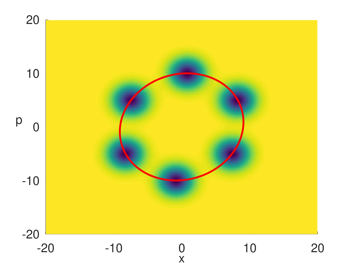
Figure 1: Husimi phase space distribution $\hat{\rho}^{{\rm(\ell c)}}(\alpha,t)$ for the limit cycle given in eq. (102) shown for six equidistant times. The center of the distribution follows the ellipse (47) shown as a red curve.

Figure 1 illustrates the long time dynamics for a system with both loss and gain, $\mu=0.6$ and $\nu=0.4$, for $\omega=1.1$, and resonant harmonic driving $\Omega=\Omega_{R}=\sqrt{\omega_{0}^{2}-\gamma^{2}}=1.0954$ with an amplitude $f_{0}=1.4$. The Husimi phase space distribution $\hat{\rho}^{{\rm(\ell c)}}(t)$ for the limit cycle given in eq. (102) is shown in the $(x,p)$-plane  ($\alpha=(\omega x+{\rm i}p)/\sqrt{2\omega}$)  for six equidistant times in the period $2\pi/\Omega$. The center of the distribution follows the ellipse (47) where $\langle\hat{x}\rangle^{{\rm(\ell c)}}(t)$ and $\langle\hat{p}\rangle^{{\rm(\ell c)}}(t)$ are given in (43) and (46).

Let us finally remark that for $\nu=0$ the limit cycle distribution turns out to be a pure coherent state, which implies that any initial distribution is driven into a coherent state. However we know that a coherent state remains coherent under the evolution, so that its limiting distribution must be necessarily coherent, with the unavoidable consequence that the limit state must be coherent.

Closing this section, we briefly look at the entropy

$$S(t)=-{\rm\,trace\,}\big{(}\hat{\rho}(t)\log\hat{\rho}(t)\big{)}\,,$$ (104)

which can be most easily evaluated by expressing the density operator in pure exponential form $\hat{\rho}=b\,{\rm e}^{\sigma(|\alpha|^{2}+\hat{n}-\alpha\hat{a}^{\dagger}-\alpha^{*}\hat{a})}$ as in (90). We then have

$$S(t) = -{\rm\,trace\,}\big{(}\hat{\rho}\,(\log b+\sigma(|\alpha|^{2}+\hat{n}-\alpha\hat{a}^{\dagger}-\alpha^{*}\hat{a}))\big{)}$$ (105)

$$= -\log b-\sigma\big{(}|\alpha|^{2}+\langle\hat{n}\rangle-\alpha\langle\hat{a}^{\dagger}\rangle-\alpha^{*}\langle\hat{a}\rangle\big{)}\,.$$

Inserting the expectation values $\langle\hat{a}\rangle=\alpha$, $\langle\hat{a}^{\dagger}\rangle=\alpha^{*}$ (see eq. (91)) and $\langle\hat{n}\rangle=1/b-1+|\alpha|^{2}$ from eqs. (82) and (85), one arrives, with $b=1-{\rm e}^{\sigma}$ and $\sigma=\log u$, at

$$S(t)=-\log(1-u(t))-\frac{u(t)}{1-u(t)}\,\log u(t)\,,$$ (106)

where $u(t)$ is given in closed form in eq. (73). Because of ${\rm d}S/{\rm d}u>0$ and the monotonicity of $u(t)$, the entropy is monotonically decreasing for $u_{0}>\nu/\mu$ and increasing for $u_{0}<\nu/\mu$. It should be pointed out, that the parameter $u(t)$, and hence the entropy $S(t)$, does only depend on the Lindblad parameters $\mu$ and $\nu$ and not at all on the driving force. In the long time limit $u(t)$ approaches $\nu/\mu$ and the resulting value $S_{\infty}$ is

$$S_{\infty}=-\frac{1}{2\gamma}\Big{(}\nu\log\nu-\mu\log\mu+2\gamma\log 2\gamma\Big{)}\,.$$ (107)

In particular we find $S_{\infty}=0$ for $\nu=0$, in accordance with the fact that the limit cycle is a coherent state. Let us also note that the entropy of the (time-dependent) limit cycle distribution $\hat{\rho}(t)$ is constant in time, which is, of course, obvious in view of the fact of the dynamics of the phase density discussed above. More results concerning the concept of entropy in context with the force-free damped harmonic oscillator can be found in [14].

5 Non-Hermitian Hamiltonian dynamics

In the preceding sections the quantum damped harmonic oscillator has been described by a Lindblad master equation. It is, however, also possible to account for damping in terms of non-Hermitian Hamiltonians. As an example, the Hamiltonian

$$\hat{H}=\tilde{\omega}\big{(}\hat{a}^{\dagger}\hat{a}+1/2\big{)}-f(t)\,\big{(}\hat{a}^{\dagger}+\hat{a}\big{)}$$ (108)

with a complex-valued frequency

$$\tilde{\omega}=\omega-{\rm i}\gamma\quad,\quad\omega,\gamma>0\,$$ (109)

has been considered in [15] in context with an analysis of a semiclassical limit of non-Hermitian quantum dynamics. Such a non-Hermitian system can be used to describe a pure loss of particles and in the following we will compare non-Hermitian and Lindblad dynamics, in particular for the case of non gain ($\nu=0$).

Let us first consider the simple force-free case $f(t)=0$. Then the solution of the Schrödinger equation ${\rm i}\frac{{\rm d}\,}{{\rm d}t}|\psi\rangle=\hat{H}|\psi\rangle$ is

$$|\psi(t)\rangle={\rm e}^{-{\rm i}\hat{H}t}|\psi_{0}\rangle={\rm e}^{-{\rm i}\tilde{\omega}(\hat{a}^{\dagger}\hat{a}+1/2)t}|\psi_{0}\rangle\,.$$ (110)

The non-Hermitian time evolution does not conserve the norm, which decays as

$$\langle\psi(t)|\psi(t)\rangle=\langle\psi_{0}|{\rm e}^{{\rm i}\tilde{\omega}^{*}(\hat{a}^{\dagger}\hat{a}+\frac{1}{2})t}{\rm e}^{-{\rm i}\tilde{\omega}(\hat{a}^{\dagger}\hat{a}+\frac{1}{2})t}|\psi_{0}\rangle=\langle\psi_{0}|{\rm e}^{-2\gamma(\hat{a}^{\dagger}\hat{a}+\frac{1}{2})t}|\psi_{0}\rangle\,.$$ (111)

Using (58) we have

$${\rm e}^{{\rm i}\tilde{\omega}^{*}(\hat{a}^{\dagger}\hat{a}+\frac{1}{2})t}\hat{a}{\rm e}^{-{\rm i}\tilde{\omega}(\hat{a}^{\dagger}\hat{a}+\frac{1}{2})t}={\rm e}^{-\gamma t}{\rm e}^{{\rm i}\tilde{\omega}^{*}\hat{n}t}\hat{a}{\rm e}^{-{\rm i}\tilde{\omega}\hat{a}^{\dagger}\hat{a}t}$$

$$\qquad\quad={\rm e}^{-\gamma t-{\rm i}\tilde{\omega}t}{\rm e}^{{\rm i}\tilde{\omega}^{*}\hat{a}^{\dagger}\hat{a}t}{\rm e}^{-{\rm i}\tilde{\omega}\hat{a}^{\dagger}\hat{a}t}\hat{a}={\rm e}^{-\gamma t-{\rm i}\tilde{\omega}t}{\rm e}^{-2\gamma\hat{a}^{\dagger}\hat{a}t}\hat{a}\,,$$ (112)

and for a coherent initial state $|\alpha_{0}\rangle$ the expectation value of $\hat{a}$ is given by

$$\langle\hat{a}\rangle_{t}=\frac{\langle\psi(t)|\hat{a}|\psi(t)\rangle}{\langle\psi(t)|\psi(t)\rangle}=\alpha_{0}\,{\rm e}^{-{\rm i}\tilde{\omega}t}=\alpha(t)\,,$$ (113)

and the expectation value of $\hat{n}$ is

$$\langle\hat{n}\rangle_{t}=|\alpha(t)|^{2}=n_{0}\,{\rm e}^{-2\gamma t}.$$ (114)

with $n_{0}=|\alpha_{0}|^{2}$. These results are in perfect agreement with the corresponding Lindblad expectation values in eq. (29) for $\nu=0$.

For the time-dependent driven system, the analysis is somewhat more involved. A closed form solution of the Schrödinger equation can be found in [15] and here we will simply copy those results. For a coherent initial state $|\alpha_{0}\rangle$, the solution is given by

$$|\psi(t)\rangle={\rm e}^{-{\rm i}\tilde{\omega}t/2+A(t)+B(t)\alpha_{0}-|\alpha_{0}|^{2}/2+|\alpha(t)|^{2}/2}\,|\alpha(t)\rangle,$$ (115)

where the parameter of the coherent state $|\alpha(t)\rangle$ is given by

$$\alpha(t)=C(t)+\alpha_{0}\,{\rm e}^{-{\rm i}\tilde{\omega}t}$$ (116)

and the coefficients $A(t)$, $B(t)$ and $C(t)$ can be found in appendix B. These terms are, however, only important if one needs to calculate explicitly the norm $\langle\psi(t)|\psi(t)\rangle$. If one is only interested in the expectation values

$$\langle\hat{A}\rangle_{t}=\frac{\langle\psi(t)|\hat{A}|\psi(t)\rangle}{\langle\psi(t)|\psi(t)\rangle}$$ (117)

most of these terms cancel, and we obtain the results

$$\langle\hat{a}\rangle_{t}=\alpha(t)=C(t)+\alpha_{0}\,{\rm e}^{-{\rm i}\tilde{\omega}t}\ ,\quad\langle\hat{n}\rangle_{t}=|\alpha(t)|^{2},$$ (118)

which reduce, of course, for $f=0$ to the expressions (113) and (114). These findings are immediately clear if one considers the renormalized density operator

$$\hat{\rho}(t)=\frac{|\psi(t)\rangle\langle\psi(t)|}{\langle\psi(t)|\psi(t)\rangle}=|\alpha(t)\rangle\langle\alpha(t)|\,.$$ (119)

The Husimi phase space distribution can be also calculated easily from the wave function (115):

$$\hat{\rho}(\alpha,t) = \frac{|\langle\alpha|\psi(t)\rangle|^{2}}{\langle\psi(t)|\psi(t)\rangle}=\big{|}\langle\alpha|\alpha(t)\rangle\big{|}^{2}={\rm e}^{-|\alpha-\alpha(t)|^{2}\,.}$$ (120)

If these results are compared with the Lindblad evolution, we find precise agreement if the Lindblad parameter $\nu$ is chosen as $\nu=0$ and therefore $\gamma=\mu$. It should be stressed, however, that this agreement is only valid for an initial coherent state, which remains coherent under the Lindblad evolution and, after renormalization, also in the non-Hermitian description.

6 Concluding remarks

In conclusion, we have described the dynamics of an elementary dynamical system, a damped and driven harmonic oscillator. This model is almost unavoidable in teaching physics, however only rarely described in quantum mechanics. Here we have presented a quite simple analysis using algebraic techniques, which allow an analytical solution of the Lindblad master equation and a calculation of important expectation values in closed form. In particular we have derived an analytic expression for the asymptotic density operator for harmonic driving, the limit cycle. Remarkably, for $\nu=0$ this is a coherent state moving along the classical limit cycle, a pure state.

The present analysis covers, however, only a special class of solutions and the derivation of a general solution remains a challenging problem for future studies as well as a deeper study of the interrelation between the Lindblad description and non-Hermitian Hamiltonians.

Appendix

Appendix A Coherent initial states

Some remarks concerning coherent state distributions may be helpful. As noted in the beginning of section 4, the exponential product

$$\hat{\rho}=Z\,{\rm e}^{\beta\hat{a}^{\dagger}}{\rm e}^{\sigma\hat{n}}{\rm e}^{\beta^{{}^{*}}\!\hat{a}}\,,$$ (121)

with real $\sigma$ and $Z=b\,{\rm e}^{-|\beta|^{2}/b}$ with $b=1-{\rm e}^{\sigma}$ describes in the limit $\sigma\rightarrow-\infty$ the pure state distribution $|\beta\rangle\langle\beta|$ of a coherent state $|\beta\rangle$. This is can be easily understood because of

$$\lim_{\sigma\rightarrow-\infty}{\rm e}^{\sigma\hat{n}}=\lim_{\sigma\rightarrow-\infty}\sum_{n=0}^{\infty}{\rm e}^{\sigma n}|n\rangle\langle n|=|0\rangle\langle 0|$$ (122)

and therefore with $Z\rightarrow{\rm e}^{-|\beta|^{2}/b}$ for $\sigma\rightarrow-\infty$

$$\lim_{\sigma\rightarrow-\infty}\hat{\rho}={\rm e}^{-|\beta|^{2}}{\rm e}^{\beta\hat{a}^{\dagger}}|0\rangle\langle 0|{\rm e}^{\beta^{*}\hat{a}}=|\beta\rangle\langle\beta|$$ (123)

(for the last equality see, e.g., [1, eq. (3.3.42)]).

An example of such a density operator is found in eq. (24) for the force-free oscillator, namely

$$\hat{\rho}(t)={\rm e}^{c(t)}\,{\rm e}^{-\log G(t)\big{(}\beta(t)\hat{a}^{\dagger}+\beta^{*}(t)\hat{a}-\hat{n}\big{)}}$$ (124)

with

$$c(t)=|\alpha_{0}|^{2}{\rm e}^{-2\gamma t}\log G(t)+\log(1-G(t))\ ,\quad\beta(t)=\alpha_{0}{\rm e}^{-(\gamma+{\rm i}\omega)t}\,,$$ (125)

where $G(t)$ is given in (20), and $\hat{\rho}(0)=|\alpha_{0}\rangle\langle\alpha_{0}|$. By means of the disentangling relations (56) this can be rewritten as an exponential product

$$\hat{\rho}(t)={\rm e}^{c^{\prime}(t)}\,{\rm e}^{\beta(t)(1-G(t))\hat{a}^{\dagger}}\,{\rm e}^{\log G(t)\,\hat{n}}\,{\rm e}^{\beta^{{}^{*}}\!(t)(1-G(t))\hat{a}}$$ (126)

with $c^{\prime}(t)=-|\beta(t)|^{2}(1-G(t))+\log(1-G(t))$. Initially we have $G(0)=0$ and $\beta(0)=\alpha_{0}$ and from the arguments above we see $\hat{\rho}(0)=|\alpha_{0}\rangle\langle\alpha_{0}|$. For $\nu=0$, where we have $G(t)=0$ for all times, we find in the same way

$$\hat{\rho}(t)=|\beta(t)\rangle\langle\beta(t)|$$ (127)

with $\beta(t)=\alpha_{0}{\rm e}^{-(\mu/2+{\rm i}\omega)t}$, i.e. the system stays in a coherent state for all times.

Appendix B Details of non-Hermitian dynamics

For convenience of the reader we reproduce here some details of the non-Hermitian dynamics from [15]. These results can be derived, e.g., by epressing the time-evolution operator as an exponential product as in section 4 or by extending the analysis of the Hermitian forced harmonic oscillator in [1, sect. 3.11] to complex frequencies. For a coherent initial state $|\alpha_{0}\rangle$ this leads to the the wave function (115), where the coefficients $A(t)$, $B(t)$ and $C(t)$ are solutions of the differential equations

$${\rm i}\dot{B}=-f{\rm e}^{-{\rm i}\tilde{\omega}t}\ ,\quad{\rm i}\dot{C}=\tilde{\omega}C-f^{*}\ ,\quad{\rm i}\dot{A}=-fC$$ (128)

with initial conditions $A(0)=B(0)=C(0)=0$, namely

$$B(t)=-{\rm i}\int_{0}^{t}{\rm d}t^{\prime}{\rm e}^{{\rm i}\tilde{\omega}t^{\prime}}f(t^{\prime})\ ,\quad C(t)=-{\rm i}\int_{0}^{t}{\rm d}t^{\prime}{\rm e}^{{\rm i}\tilde{\omega}(t-t)}f^{*}(t^{\prime})$$

$$A(t)={\rm i}\int_{0}^{t}{\rm d}t^{\prime}\,f(t^{\prime})C(t^{\prime}).$$ (129)

For harmonic driving force $f(t)=\tilde{f}_{0}\cos\Omega t$ these solutions are given by

$$B(t)=\frac{-f_{0}}{2(\tilde{\omega}^{2}-\Omega^{2})}\Big{\{}(\tilde{\omega}+\Omega){\rm e}^{-{\rm i}(\tilde{\omega}-\Omega)t}+(\tilde{\omega}-\Omega){\rm e}^{-{\rm i}(\tilde{\omega}+\Omega)t}-2\tilde{\omega}\Big{\}}$$ (130)

$$C(t)=\frac{f_{0}}{2(\tilde{\omega}^{2}-\Omega^{2})}\Big{\{}(\tilde{\omega}-\Omega){\rm e}^{{\rm i}\Omega t}+(\tilde{\omega}+\Omega){\rm e}^{-{\rm i}\Omega t}-2\tilde{\omega}{\rm e}^{-{\rm i}\tilde{\omega}t}\Big{\}}$$ (131)

$$A(t)=\frac{f^{2}_{0}}{4(\tilde{\omega}^{2}-\Omega^{2})}\Big{\{}1+2{\rm i}\tilde{\omega}t+\frac{\tilde{\omega}+\Omega}{2\Omega}{\rm e}^{-{\rm i}(\tilde{\omega}-\Omega)t}-\frac{\tilde{\omega}-\Omega}{2\Omega}{\rm e}^{-{\rm i}(\tilde{\omega}+\Omega)t}$$

$$\qquad\quad+\frac{2\tilde{\omega}}{\tilde{\omega}^{2}-\Omega^{2}}\Big{(}(\tilde{\omega}+\Omega){\rm e}^{-{\rm i}(\tilde{\omega}-\Omega)t}+(\tilde{\omega}-\Omega){\rm e}^{-{\rm i}(\tilde{\omega}+\Omega)t}-2\tilde{\omega}\Big{)}\Big{\}}.$$ (132)

(Note that the factor $2$ in the denominator in eq. (130) is missing in [15].)