Pion off-shell electromagnetic form factors: Data extraction and model analysis

Abstract

We investigate the pion electromagnetic half-off-shell form factors, which parametrize the matrix element of the charged pion electromagnetic current with one leg off-mass-shell and the other leg on-mass-shell, using an exactly solvable manifestly covariant model of a $(3+1)$ dimensional fermion field theory. The model provides a three-dimensional imaging of the two off-shell pion form factors $F_{1}$ and $F_{2}$ as a function of $(Q^{2},t)$, which are related to each other satisfying the Ward-Takahashi identity. The normalization of the renormalized charge form factor $F_{1}$ is fixed by $F_{1}(Q^{2}=0,t=m^{2}_{\pi})=1$ while the other form factor $F_{2}$ vanishes, i.e. $F_{2}(Q^{2},t=m^{2}_{\pi})=0$ for any value of $Q^{2}$ due to the time-reversal invariance of the strong interaction. We define the new form factor $g(Q^{2},t)=F_{2}(Q^{2},t)/(t-m^{2}_{\pi})$ and find that $g(Q^{2},t)$ can be measurable in the on-mass-shell limit. In particular, $g(Q^{2}=0,t=m^{2}_{\pi})$ is related with the pion charge radius. We also compare our form factors with the data extracted from the pion electroproduction reaction for both the off-shell region ($t<0$) and the on-shell limit ($t\rightarrow m_{\pi}^{2}$).

I Introduction

Electromagnetic (EM) form factors of hadrons are the important physical observables providing the EM information on the bound-state properties of hadrons and their internal structures of quarks and gluons. The pion is the simplest hadronic system, the valence structure of which is a bound state of a quark and an antiquark, and is known to be parametrized by a single on-mass-shell (or simply on-shell) EM form factor, $F_{\pi}(Q^{2})$, which depends on the 4-momentum squared $q^{2}(=-Q^{2})$ of the virtual photon.

The form factor $F_{\pi}(Q^{2})$ for the low spacelike momentum transfers ($Q^{2}<0.3$ GeV²) has been measured directly by elastic scattering of high-energy mesons off atomic electrons Dally1 ; Dally2 ; Amen1 ; Amen2 . However, the extraction of $F_{\pi}(Q^{2})$ to higher $Q^{2}$ regions through elastic scattering is very difficult experimentally mainly due to the limitation of the availability of accelerators to produce high-energy and high-current beams of unstable particles and detectors for identifying and measuring the scattered particles at very forward angles Marco . Thus, $F_{\pi}(Q^{2})$ for the higher $Q^{2}$ values has been extracted from the pion electroproduction reaction by exploiting the nucleon’s pion cloud as a target, which may be regarded as the exclusive version of the Sullivan process Sull . That is, $F_{\pi}(Q^{2})$ has been extracted from the measurements of the cross sections for the reaction ${}^{1}{\rm H}(e,e^{\prime}\pi^{+})n$ (see Fig. 1) up to values of $Q^{2}=3.91$ GeV² Blok2008 ; Huber2008 ; JLab3 ; JLab4 ; JLab5 . The longitudinal part of the cross section from the pion electroproduction encodes the meson exchange process, in which the virtual photon couples to a virtual pion inside the nucleon. This process is expected to dominate at small values of the 4-momentum transfer $t(<0)$, allowing for the determination of the pion form factor.

Figure 1: $ep\rightarrow e^{\prime}\pi^{+}n$ scattering.

However, the main problem in using the electroproduction process as a tool for accessing a “pion target” is that the pions in a nucleon’s cloud are not real (on-shell) but virtual (off-shell) particles. Accordingly, one cannot access the form factor at the exact pion pole in the actual experiment as the extrapolation to $t\to m_{\pi}^{2}$ involves the disallowed kinematic region of the electroproduction ($t<0$). This may raise some questions about the validity of the extrapolation from the off-shell results to the on-shell limit. Furthermore, the EM structure of the off-shell hadron is more complicated than the on-shell hadron and involves more form factors Rudy ; Weiss ; Craig ; CraigK ; N1 ; N2 ; N3 ; N4 ; N5 . For instance, the off-shell EM structure of the pseudoscalar meson Rudy ; Weiss requires two form factors Nis ; Bar , which are related by the Ward-Takahashi identity(WTI) Ward ; Taka . The off-shell electromagnetic form factors for the boson bound state have been calculated in Naus1998 using the light-front field theory and the nonvanishing zero modes were found to be crucial to preserve the WTI. While there have been some theoretical studies on the off-shell pion EM form factors using the chiral perturbation theory Rudy , Nambu-Jona-Lasinio model Weiss , and the continuum methods for the strong-interaction bound-state problem Craig ; CraigK , a further systematic study on the off-shell form factors of the pion is still required.

In this work, we explore the electromagnetic off-shell effects for the pion using an exactly solvable manifestly covariant model of $(3+1)$-dimensional fermion field theory and compare the two off-shell form factors $F_{1}(Q^{2},t)$ and $F_{2}(Q^{2},t)$ with the data extracted from the pion electroproduction reaction Blok2008 ; Huber2008 . The aim of this paper is to provide at least a clear example of demonstration discussing the validity of the extrapolation of the off-shell results ($t\neq m_{\pi}^{2}$) to the on-shell limit ($t=m_{\pi}^{2}$) for the pion. We exhibit $F_{1(2)}(Q^{2},t)$ not only for the spacelike region ($Q^{2}>0$) but also for the timelike region ($Q^{2}<0$), providing the three-dimensional (3D) imaging of $F_{1}$ and $F_{2}$ in terms of $(Q^{2},t)$ values.

We organize this work as follows. In Sec. II, we review the formulation of $F_{1}$ and $F_{2}$ satisfying the WTI, in which two form factors are necessary to define the off-shell matrix elements of the pion EM current. In addition, we provide a sum rule, coined here as the master equation, which we obtain from the WTI that the form factors must obey regardless of whether they are on-shell or off-shell. While $F_{2}(Q^{2},t)$ is zero as $t\to m^{2}_{\pi}$, we find a new measurable form factor in the on-shell limit by defining $g(Q^{2},t)=F_{2}(Q^{2},t)/(t-m^{2}_{\pi})$. Especially, we show that $g(Q^{2}=0,t=m^{2}_{\pi})$ is found to be related with the pion charge radius. In Sec. III, we present the analytic covariant model calculation of $F_{1}$ and $F_{2}$ confirming that the model satisfies the master equation given by Eq.(11) as well as the WTI. We also discuss the charge renormalization for $F_{1}(Q^{2},t)$ together with the relation between the coupling $g_{\pi q{\bar{q}}}$ of the $\pi q\bar{q}$ vertex and the pion decay constant $f_{\pi}$. In Sec. IV, we present 3D imaging of $F_{1}(Q^{2},t),F_{2}(Q^{2},t)$ and $g(Q^{2},t)$ and compare them with the available data extracted from the pion electroproduction reaction for both the off-shell region ($t<0$) and the on-shell limit ($t\rightarrow m_{\pi}^{2}$). A summary of the main results follows in Sec. V. In the Appendix, the explicit derivation of Eqs. (19) and  (20) is briefly summarized.

Figure 2: Electromagnetic charged pion scattering with the form factors depicted by the black blob.

II Off-shell Pion Electromagnetic Form Factors

Using the invariance of the strong interaction under charge conjugation, one finds that the electromagnetic form factors of antiparticles are just the negative of those of the particles. Therefore, the $\pi^{0}$ and $\eta$ do not have any electromagnetic form factors even for the off-mass-shell case. However, the charged pions allow the electromagnetic form factors depicted in Fig. 2. The most general parametrization of the vertex function $\Gamma^{\mu}$ for the off-shell electromagnetic form factors of the charged pion is given in terms of the initial and final 4-momenta, $p^{\mu}$ and  $p^{\prime\mu}$, as Rudy

$$\Gamma_{\mu}(p,p^{\prime})=~{}(p^{\prime}+p)_{\mu}~{}G_{1}(q^{2},p^{2},p^{\prime 2})+q_{\mu}~{}G_{2}(q^{2},p^{2},p^{\prime 2})~{},$$ (1)

where $q=p^{\prime}-p$ is the 4-momentum transfer of the virtual photon at the vertex. This off-shell vertex satisfies the WTI Rudy

$$q^{\mu}\Gamma_{\mu}(p,p^{\prime})=~{}\Delta^{-1}(p^{\prime})-\Delta^{-1}(p),$$ (2)

where

$$\Delta(p)~{}=~{}\frac{1}{p^{2}-m^{2}_{\pi}-\Pi(p^{2})+\imath\epsilon},$$ (3)

is the full renormalized propagator Rudy and the renormalized pion self-energy $\Pi(p^{2})$ is constrained by the on-mass-shell condition $\Pi(m^{2}_{\pi})=0$.

From the WTI given by Eq. (2), we get the following constraint on the off-shell form factors $G_{1}$ and $G_{2}$:

$$(p^{\prime 2}-p^{2})G_{1}(q^{2},p^{2},p^{\prime 2})+q^{2}G_{2}(q^{2},p^{2},p^{\prime 2})$$

$$=\Delta^{-1}(p^{\prime})-\Delta^{-1}(p).$$ (4)

In particular, for the case of real photons (i.e. $q^{2}=0$) and for the half-off-shell form factor, namely, the final state being on-mass shell $p^{\prime 2}=m^{2}_{\pi}$ with $\Delta^{-1}(p^{\prime})=0$, one finds from Eq. (II) that

$$\Delta^{-1}(p) = (p^{2}-m^{2}_{\pi})G_{1}(0,p^{2},m^{2}_{\pi})$$ (5)

$$= (p^{2}-m^{2}_{\pi})G_{1}(0,m^{2}_{\pi},p^{2}).$$

Thus, the form factor normalization $G_{1}(0,m^{2}_{\pi},m^{2}_{\pi})=1$, which can be interpreted as the charge of the pion, is attained in the on-shell limit $(p^{2}=m^{2}_{\pi}$) of the initial state since ${\rm lim}_{p^{2}\to m^{2}_{\pi}}[(p^{2}-m^{2}_{\pi})\Delta(p)]^{-1}=1$. However, the extension to $G_{1}(0,m^{2}_{\pi},p^{2})=1$ for the half-off-shell case ($p^{2}\neq m^{2}_{\pi}$) is in general not possible due to the nonvanishing $\Pi(p^{2})$ term. It is also interesting to note that $G_{1}(q^{2},p^{2},p^{\prime 2})=G_{1}(q^{2},p^{\prime 2},p^{2})$ and $G_{2}(q^{2},p^{2},p^{\prime 2})=-G_{2}(q^{2},p^{\prime 2},p^{2})$, respectively, from Eq. (II) and the time-reversal invariance of the strong interaction.

From Eq. (II), the off-shell form factor $G_{1}(q^{2},p^{2},p^{\prime 2})$ in the real photon limit ($q^{2}=0$) is given by

$$G_{1}(0,p^{2},p^{\prime 2})=\frac{\Delta^{-1}(p^{\prime})-\Delta^{-1}(p)}{p^{\prime 2}-p^{2}}.$$ (6)

Substituting Eq. (6) back into Eq. (II), one obtains

$$G_{2}(q^{2},p^{2},p^{\prime 2})=\frac{(p^{\prime 2}-p^{2})[G_{1}(0,p^{2},p^{\prime 2})-G_{1}(q^{2},p^{2},p^{\prime 2})]}{q^{2}}.$$ (7)

In the case of the pion initial state being off-mass-shell but the final state being on-mass-shell, i.e. $p^{2}=t$ and $p^{\prime 2}=m^{2}_{\pi}$, Eq. (7) becomes Rudy

$$F_{2}(Q^{2},t)=\frac{t-m^{2}_{\pi}}{Q^{2}}\,\left[F_{1}(0,t)-F_{1}(Q^{2},t)\right]\,,$$ (8)

where $F_{i}(Q^{2},t)\equiv G_{i}(q^{2},t,m^{2}_{\pi})(i=1,2)$ and $Q^{2}=-q^{2}$. We note that $F_{2}(Q^{2},t)=0$ if both initial and final pions are on-mass-shell (i.e. $p^{2}=p^{\prime 2}=m^{2}_{\pi}$), which is consistent with the antisymmetric property of $G_{2}$, i.e. $G_{2}(Q^{2},p^{2},p^{\prime 2})=-G_{2}(Q^{2},p^{\prime 2},p^{2})$. The normalization of $F_{1}$ is fixed by requiring $F_{1}(Q^{2}=0,t=m^{2}_{\pi})=1$ as we discussed earlier. The renormalized pion self-energy $\Pi(t)$ is also related to the off-shell pion form factor $F_{1}(Q^{2}=0,t)$ as $\Pi(t)=(t-m^{2}_{\pi})\left[1-F_{1}(0,t)\right]$, assuring the on-mass-shell condition $\Pi(t=m^{2}_{\pi})=0$ mentioned earlier. We have checked the chiral perturbation theory up to one loop Rudy and confirmed that the off-shell pion form factors obtained in Ref. Rudy satisfy the general formula given by Eq.  (8), as it should be.

From Eqs. (1) and (8), the half-on-shell ($p^{\prime 2}=m^{2}_{\pi}$) and half-off-shell ($p^{2}=t<0$) pion-photon vertex can be effectively given by

$$\Gamma_{\mu}=(p^{\prime}+p)_{\mu}~{}F_{1}(Q^{2},t)+q_{\mu}\frac{(t-m^{2}_{\pi})}{Q^{2}}~{}[F_{1}(0,t)-F_{1}(Q^{2},t)].$$ (9)

In the elastic electron scattering, the contraction of the second term in Eq.(9) with the electron current vanishes due to the current conservation. It suggests that $F_{2}(Q^{2},t)$ given by Eq.(8) cannot be directly measured in the electroproduction process due to the transversality of the electron current. We note, however, that the ratio of $F_{2}(Q^{2},t)$ to $t-m^{2}_{\pi}$ is nonzero in the limit of $t\to m^{2}_{\pi}$ although $F_{2}(Q^{2},t)$ itself goes to zero as $t\to m^{2}_{\pi}$. To exhibit this more clearly, let us define the new form factor

$$g(Q^{2},t)\equiv\frac{F_{2}(Q^{2},t)}{t-m^{2}_{\pi}}\,.$$ (10)

Then, the off-shell form factor sum rule given by Eq. (8) can be rewritten as

$$F_{1}(Q^{2},t)-F_{1}(0,t)+Q^{2}g(Q^{2},t)=0\,.$$ (11)

Taking the derivative of Eq. (11) with respect to $Q^{2}$, one finds the following evolution equation:

$$\frac{\partial}{\partial Q^{2}}F_{1}(Q^{2},t)\,+\,g(Q^{2},t)+Q^{2}\frac{\partial g(Q^{2},t)}{\partial Q^{2}}\,=\,0\,.$$ (12)

We should note that $g(Q^{2}=0,t=m^{2}_{\pi})$ is associated with the charge radius of the pion elastic form factor. In other words, since

$$g(Q^{2}=0,m^{2}_{\pi})=-\frac{\partial}{\partial Q^{2}}F_{1}(Q^{2}=0,m^{2}_{\pi})=\frac{1}{6}\langle r^{2}_{\pi}\rangle$$ (13)

in the on-mass-shell limit $t=m^{2}_{\pi}$ and at $Q^{2}=0$, we get the on-mass-shell solution for $g(Q^{2},t)$

$$g(Q^{2},m^{2}_{\pi})=\frac{1}{6}\langle r^{2}_{\pi}\rangle\,+\,\alpha\;Q^{2}+\,\cdots\,,$$ (14)

where $\alpha$ is determined by expanding $\frac{\partial}{\partial Q^{2}}F_{1}(Q^{2},t)$ and $\frac{\partial}{\partial Q^{2}}g(Q^{2},t)$ in $Q^{2}$ around $Q^{2}=0$. Effectively, the master equation given by Eq.(11) allows us to extract both off-shell form factors simultaneously while the electroproduction process cannot directly measure $F_{2}(Q^{2},t)$. Interestingly, however, neither of the two form factors $F_{1}(Q^{2},t)$ and $g(Q^{2},t)$ vanishes even in the on-mass-shell limit $t=m^{2}_{\pi}$.

Furthermore, we can continue elaborating the master equation given by Eq. (11), taking the derivative in $t$,

$$\frac{\partial}{\partial t}F_{1}(Q^{2},t)\,-\,\frac{\partial F_{1}(0,t)}{\partial t}\,+Q^{2}\frac{\partial g(Q^{2},t)}{\partial t}\,=\,0\,,$$ (15)

and the master equation given by Eq. (12), taking the derivative in $t$,

$$\frac{\partial^{2}}{\partial t\partial Q^{2}}F_{1}(Q^{2},t)\,+\,\frac{\partial g(Q^{2},t)}{\partial t}\,+Q^{2}\frac{\partial^{2}g(Q^{2},t)}{\partial t\partial Q^{2}}\,=\,0\,.$$ (16)

The form factor $g(Q^{2},m^{2}_{\pi})$ is the new observable in the on-mass-shell limit besides the usual charge form factor $F_{1}(Q^{2},m^{2}_{\pi})$ and should be measurable in the experiment of pion electroproduction. In the next section, we shall explicitly show all those properties of the off-shell pion form factors using the exactly solvable manifestly covariant model.

III Manifestly Covariant Model Calculation

III.1 Model description: Theory

Figure 3: Feynman triangle diagram for the pion off-shell form factors.

The vertex function for the initial off-shell ($p^{2}=t$) and final on-shell ($p^{\prime 2}=m^{2}_{\pi}$) $q{\bar{q}}$ bound-state pion coupled to the virtual photon with the 4-momentum $q$ in the fermion field theory can be calculated using the tree-level diagram (see Fig. 3) as

$$\Gamma^{\mu}=iN_{c}g^{2}_{\pi q{\bar{q}}}\int\frac{d^{4}k}{(2\pi)^{4}}\frac{S^{\mu}}{N_{k}N_{k+q}N_{p-k}},$$ (17)

where $N_{c}$ is the number of colors and $g_{\pi q{\bar{q}}}$ corresponds to the coupling constant of the $\pi q{\bar{q}}$ vertex. The denominators $N_{k}=k^{2}-m^{2}_{q}+i\epsilon$, $N_{k+q}=(k+q)^{2}-m^{2}_{q}+i\epsilon$, and $N_{p-k}=(p-k)^{2}-m^{2}_{q}+i\epsilon$ come from the intermediate quark and antiquark propagators with the constituent quark mass $m_{q}=m_{\bar{q}}$, respectively. The trace term $S^{\mu}$ in Eq. (17) is given by

$$S^{\mu}={\rm Tr}[\gamma_{5}(\not\!k+\not\!q+m_{q})\gamma^{\mu}(\not\!k+m_{q})\gamma_{5}(\not\!k-\not\!p+m_{q})],$$ (18)

and the explicit calculation of the triangle loop using the Feynman parametrization and the dimensional regularization in $d(=4-2\epsilon)$-dimensions is summarized in Appendix.

From the definition of $\Gamma^{\mu}=(p^{\prime}+p)^{\mu}F_{1}(Q^{2},t)+q^{\mu}F_{2}(Q^{2},t)$, we then obtain the two form factors $F_{1}(Q^{2},t)$ and $F_{2}(Q^{2},t)$ as

$$F_{1}(Q^{2},t) = -\frac{N_{c}g^{2}_{\pi q{\bar{q}}}}{8\pi^{2}}\int^{1}_{0}\;dx\int^{x}_{0}\;dy$$

$$\times\biggl{[}(1+3y)\biggl{(}\gamma-\frac{1}{\epsilon}+\frac{1}{2}+{\rm Log}C\biggr{)}+\frac{\alpha}{C}\biggr{]},$$

and

$$F_{2}(Q^{2},t) = -\frac{N_{c}g^{2}_{\pi q{\bar{q}}}}{8\pi^{2}}\int^{1}_{0}\;dx\int^{x}_{0}\;dy$$ (20)

$$\times\biggl{[}3(1-2x+y){\rm Log}C+\frac{2\beta-\alpha}{C}\biggr{]},$$

where $\gamma\simeq 0.577$ is the Euler-Mascheroni constant and

$$\alpha = (1+y)(E^{2}-m^{2}_{q})-q\cdot E+2yp\cdot E-yq\cdot p,$$

$$\beta = (1-x+y)(E^{2}-m^{2}_{q})+(1-2x+2y)p\cdot E+(x-y)q\cdot p,$$

and $C$ and $E$ are given in Appendix A. We should note that the form factor $F_{2}(Q^{2},t)$ is free from the UV divergence since the integration of $(1-2x+y)$ multiplied by the constant factor $(\gamma-1/\epsilon+1/2)$ gives zero in Eq. (20).

On the other hand, the form factor $F_{1}(Q^{2},t)$ at $(Q^{2}=0,t=m^{2}_{\pi})$ is obtained as

$$F_{1}(0,m^{2}_{\pi}) = -\frac{N_{c}g^{2}_{\pi q{\bar{q}}}}{8\pi^{2}}\biggl{[}{\rm Log}(m^{2}_{q})+\gamma-\frac{1}{\epsilon}-\frac{7}{6}$$

$$-\frac{2(m^{2}_{\pi}-2m^{2}_{q})}{m_{\pi}\sqrt{4m^{2}_{q}-m^{2}_{\pi}}}\tan^{-1}\biggl{(}\frac{m_{\pi}}{\sqrt{4m^{2}_{q}-m^{2}_{\pi}}}\biggr{)}\biggr{]}.$$

As the loop correction to the charge form factor $F_{1}(Q^{2},t=m^{2}_{\pi})$ must vanish at $Q^{2}=0$, the charge at $Q^{2}=0$ is given by a subtraction to the contribution by the loop integral. We thus redefine the renormalized charge form factor as

$$F^{\rm ren}_{1}(Q^{2},t)=1+[F_{1}(Q^{2},t)-F_{1}(0,m^{2}_{\pi})],$$ (23)

where the loop correction in the square bracket vanishes at $Q^{2}=0$ and $t=m_{\pi}^{2}$ and the normalization of the electric charge is fixed by $F^{\rm ren}_{1}(0,t=m^{2}_{\pi})=1$.

In this subtractive charge renormalization, the coupling constant $g_{\pi q{\bar{q}}}$ is still arbitrary and could become a free parameter to find the best fit for the form factors from the point of view of the phenomenological application. The coupling constant $g_{\pi q{\bar{q}}}$ is, however, related to the pseudoscalar coupling of the pion vis-á-vis Partially Conserved Axial Current. Indeed, the coupling $g_{\pi q{\bar{q}}}$ may be determined from the comparison of the on-shell pion decay constant $f_{\pi}$ defined by

$$\langle 0|{\bar{q}}\gamma^{\mu}\gamma_{5}q|\pi(p)\rangle=if_{\pi}p^{\mu},$$ (24)

where $f_{\pi}$ is obtained by the same model as

$$f_{\pi} = -\frac{N_{c}g_{\pi q{\bar{q}}}}{4\pi^{2}}m_{q}\biggl{[}\gamma-\frac{1}{\epsilon}-\frac{3}{2}+{\rm Log}(m^{2}_{q})$$ (25)

$$+\frac{2}{m_{q}}\sqrt{4m^{2}_{q}-m^{2}_{\pi}}\tan^{-1}\biggl{(}\frac{m_{\pi}}{\sqrt{4m^{2}_{q}-m^{2}_{\pi}}}\biggr{)}\biggr{]}.$$

Dividing Eq. (III.1) by Eq. (25), we obtain

$$\frac{g_{\pi q{\bar{q}}}}{2m_{q}}=\frac{F_{1}(0,m^{2}_{\pi})}{f_{\pi}}+{\cal O}(\epsilon).$$ (26)

This may motivate to relate $g_{\pi q{\bar{q}}}$ with $m_{q}$ and $f^{\rm Exp}_{\pi}=130$ MeV by taking the right hand side of Eq. (26) as $\frac{F_{1}^{\rm ren}(0,m^{2}_{\pi})}{f_{\pi}^{\rm Exp}}$ with $F_{1}^{\rm ren}(0,m^{2}_{\pi})=1$. In our numerical calculation, however, we take $g_{\pi q{\bar{q}}}$ as another free parameter in addition to $m_{q}$ for the best fit of the model calculation compared to the experimental data and examine whether the attained value of $g_{\pi q{\bar{q}}}$ is consistent with the value of $2m_{q}/f^{\rm Exp}_{\pi}$.

III.2 Model description: Numerical results

Figure 4: Proof of the WTI given by Eq. (8) for the off-shell $\pi^{+}$ obtained from $m_{q}=0.16$ GeV and $g_{\pi q{\bar{q}}}=1.11(2m_{q}/f^{\rm Exp}_{\pi})$ with fixed $t=-m^{2}_{\pi}$ value for $-1\leq Q^{2}\leq 1$ GeV².

The exactly solvable model with the half-off-shell form factors given by Eqs.  (III.1) and (20) is quantitatively explored in this subsection. In our numerical calculation, we tried to find the best fits of the form factor $F^{\rm ren}_{1}(Q^{2},t)$ compared to the experimental data $F^{\rm Exp}_{1}(Q^{2},t)$ for both the off-shell pion ($t\neq m^{2}_{\pi}$) (see Table 1) and the on-shell pion ($t=m^{2}_{\pi}$) as we shall show in Fig. 9 by adjusting our model parameters $(m_{q},g_{\pi q{\bar{q}}})$. We found the optimum ranges of quark masses, $0.12\leq m_{q}\leq 0.16$ GeV, and the best-fit for the coupling constants, $g_{\pi q{\bar{q}}}=(1.32,1.20,1.11)(2m_{q}/f^{\rm Exp}_{\pi})$ for $m_{q}=(0.12,0.14,0.16)$ GeV, respectively. That is, our phenomenological best fit coupling constants $g_{\pi q{\bar{q}}}$ are not much different from the values of $2m_{q}/f^{\rm Exp}_{\pi}$ and we check the sensitivity of the coupling $g_{\pi q{\bar{q}}}$ for given quark mass as we shall show in Fig. 9. From now on, we shall denote our results for the renormalized form factor $F^{\rm ren}_{1}(Q^{2},t)$ as $F_{1}(Q^{2},t)$ for convenience.

In Fig. 4, we provide the explicit proof of the WTI given by Eq. (8) with the two off-shell form factors $F_{1}$ and $F_{2}$ computed independently using $m_{q}=0.16$ GeV and $g_{\pi q{\bar{q}}}=1.11(2m_{q}/f^{\rm Exp}_{\pi})$ with a fixed $t=-m^{2}_{\pi}$ value for $-1\leq Q^{2}\leq 1$ GeV². Note here that we cover both timelike $(Q^{2}=-q^{2}<0)$ and spacelike $(Q^{2}>0$) regions. The timelike result is obtained from the analytic continuation by changing $Q^{2}$ to $-Q^{2}$ in the form factors of the spacelike region and vice versa. The solid, dashed, and dotted lines represent the results of $|(m_{\pi}^{2}-t)[F_{1}(0,t)-F_{1}(Q^{2},t)]|$, ${\rm Re}[(m_{\pi}^{2}-t)[F_{1}(0,t)-F_{1}(Q^{2},t)]]$, and ${\rm Im}[(m_{\pi}^{2}-t)[F_{1}(0,t)-F_{1}(Q^{2},t)]]$, respectively. Our independent calculations of $|q^{2}F_{2}(Q^{2},t)|$ (circle), ${\rm Re}[q^{2}F_{2}(Q^{2},t)]$ (square) and ${\rm Im}[q^{2}F_{2}(Q^{2},t)]$ (diamond) shown in Fig. 4 prove explicitly that our model calculation satisfies the WTI given by Eq. (8).

The kink in Fig. 4 of the timelike region is the point where the threshold starts at $q^{2}=4m^{2}_{q}$. At $q^{2}=4m^{2}_{q}$, the imaginary parts of the form factors start to develop, where the $q\bar{q}$ continuum begins in the model. Although our analytic covariant model is too simple to illustrate the timelike region $Q^{2}<0$ lacking the more realistic feature of the vector meson resonances observed experimentally (see e.g. Refs. PedlarPRL05 ; SethPRL13 ), it may provide at least a theoretical tool to discuss the off-mass-shell aspect of the charged pion form factors involved in the electroproduction process, satisfying the master equation given by Eq.(11) derived from the general WTI given by Eq.(2).

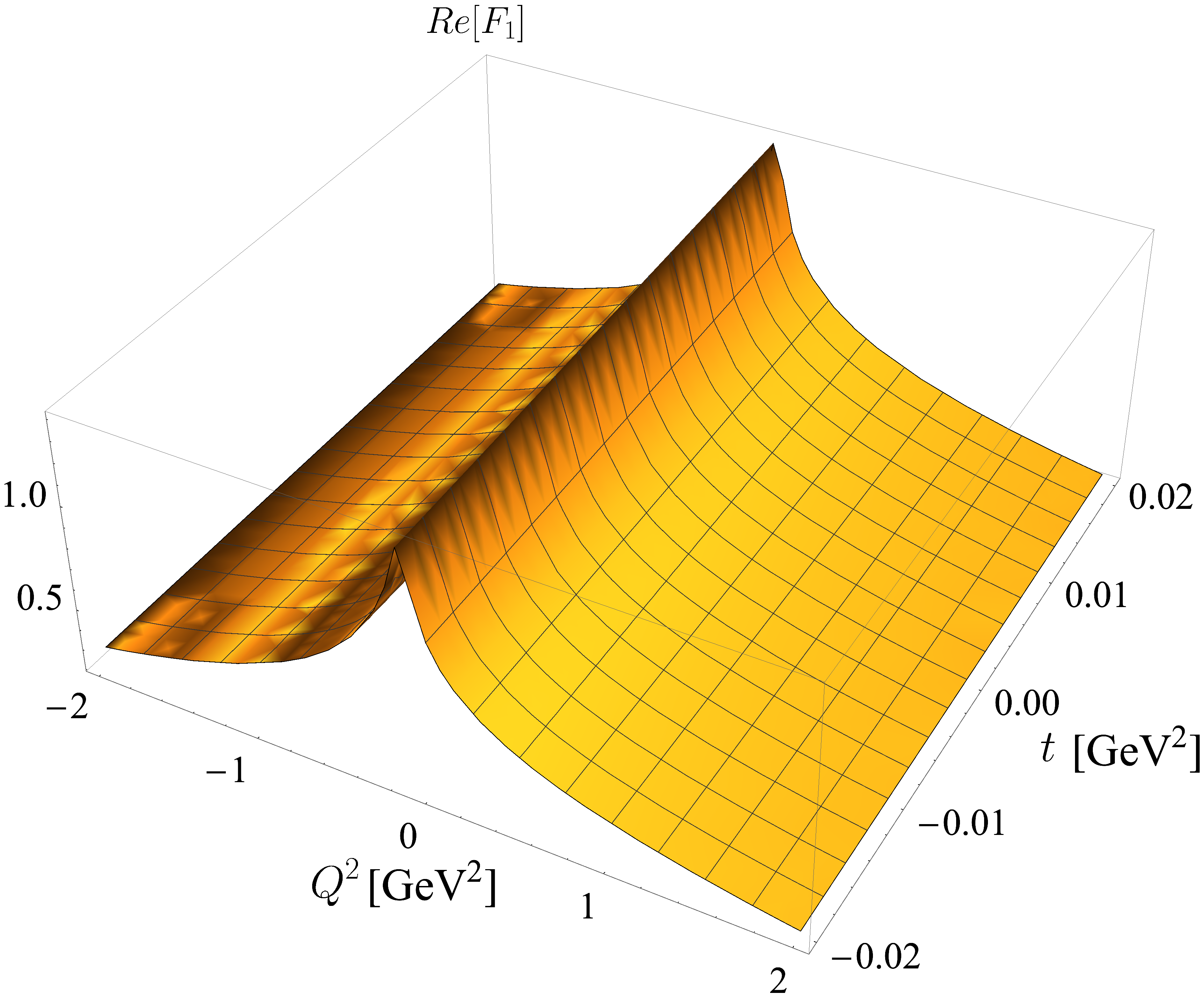
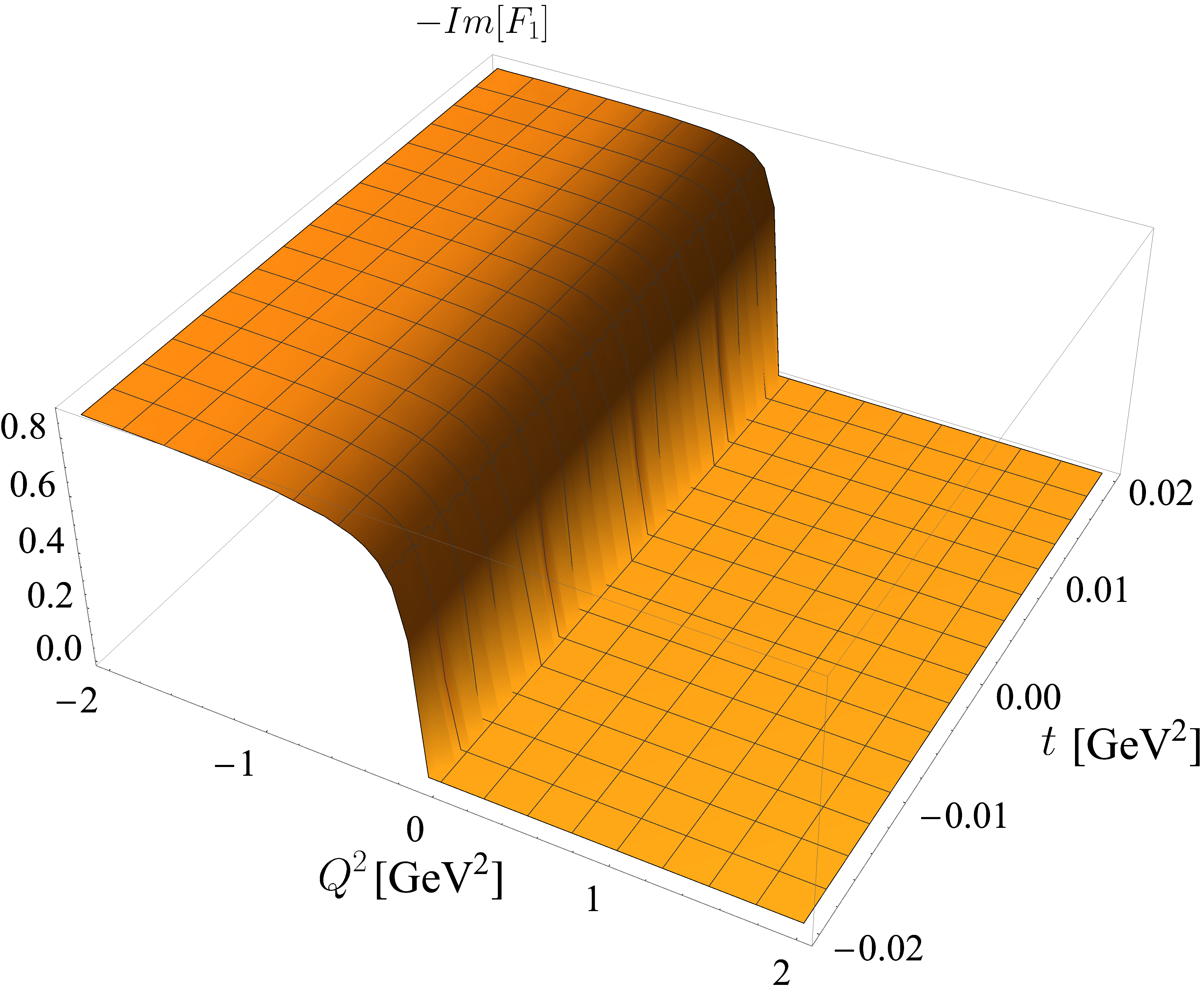
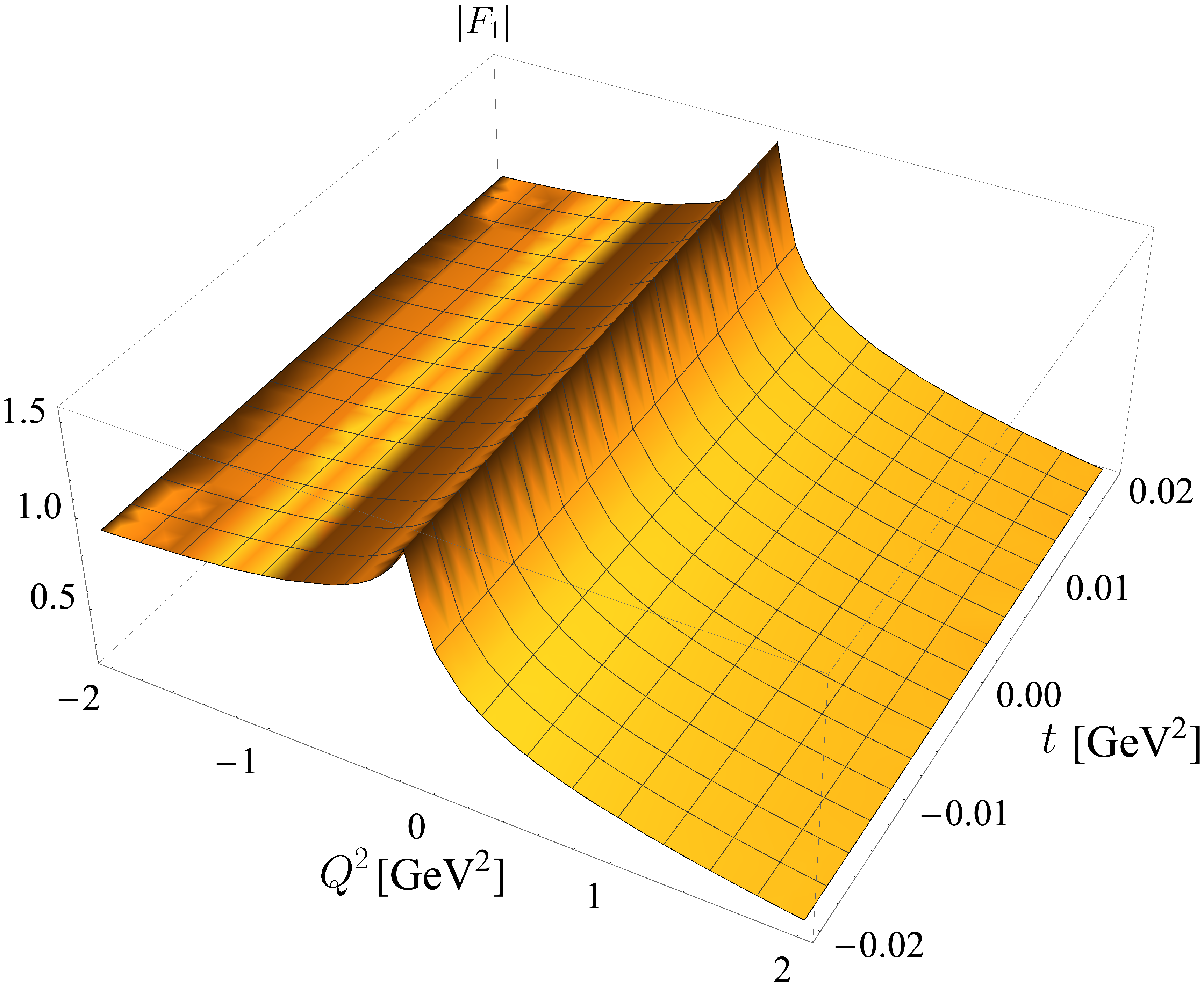
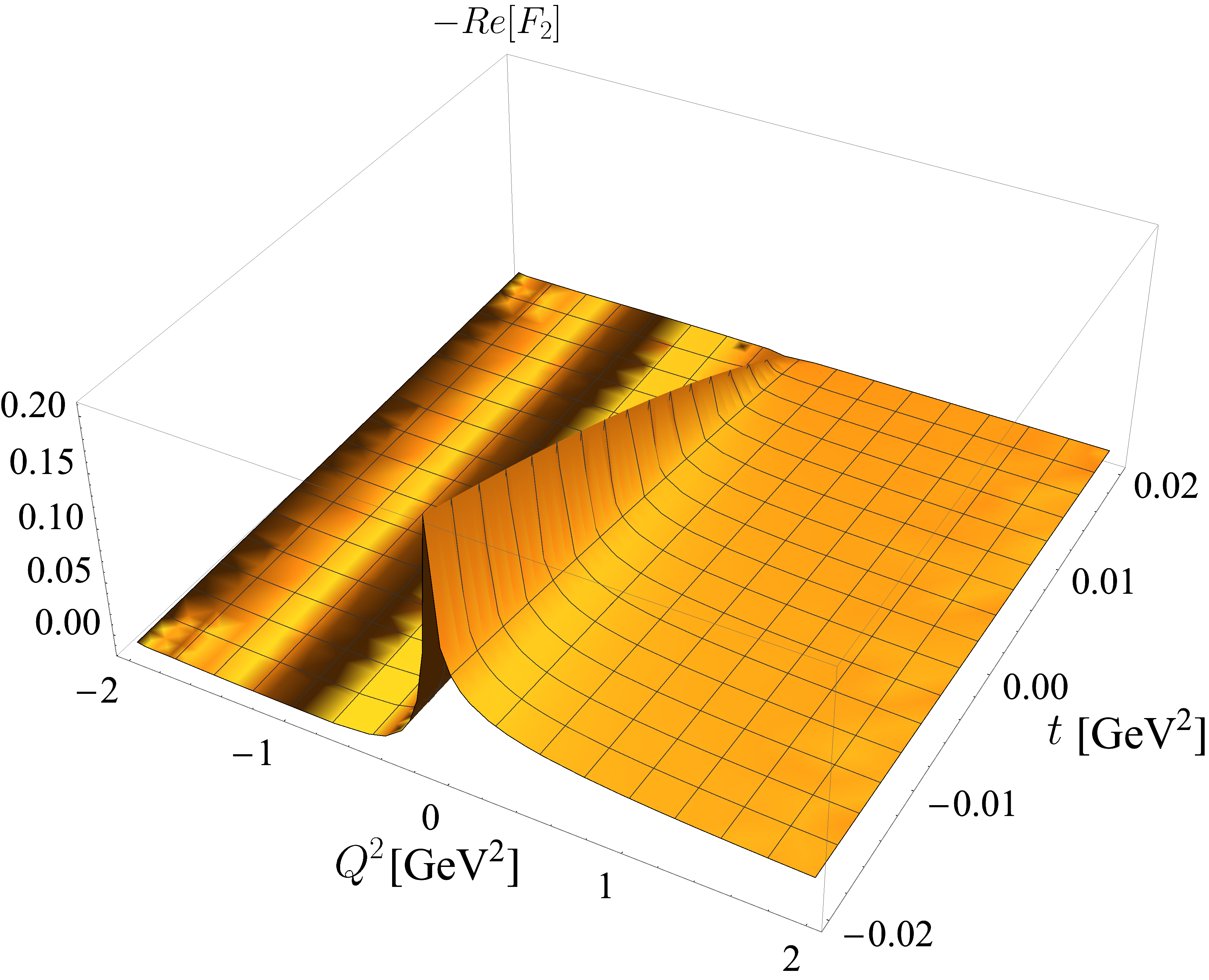
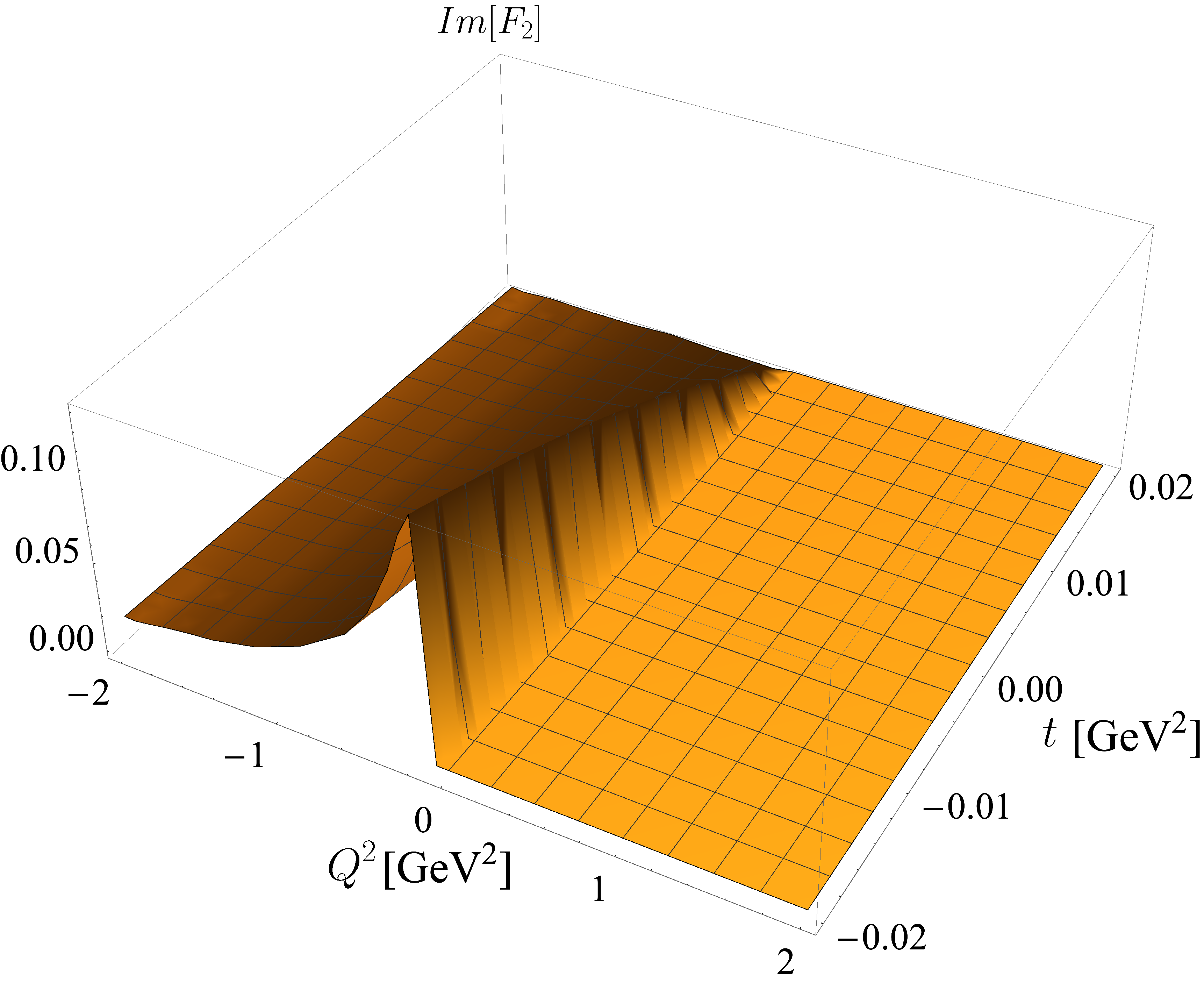
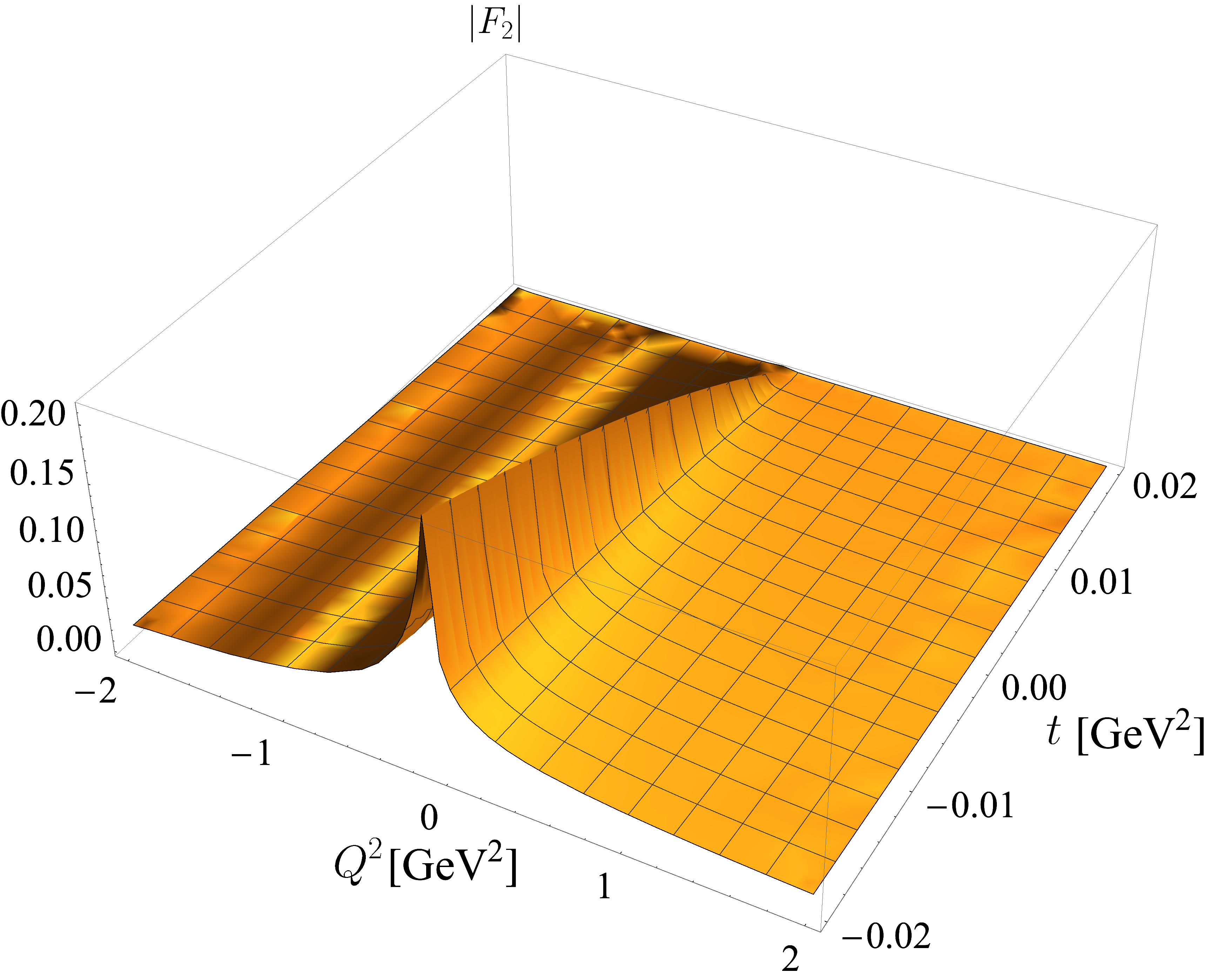
Figure 5: The 3D plots of $F_{1}(Q^{2},t)$ (upper panel) and $F_{2}(Q^{2},t)$ (lower panel) for $-2\leq Q^{2}\leq 2$ GeV² and $-m^{2}_{\pi}\leq t\leq m^{2}_{\pi}$ GeV². Left, middle, and right panels represent the results of Re[$F_{i}$], Im[$F_{i}$], and $|F_{i}|$ ($i=1,2$), respectively. The used model parameters are $m_{q}=0.16$ GeV and $g_{\pi q{\bar{q}}}=1.11(2m_{q}/f^{\rm Exp}_{\pi})$.

The overall landscape of the half-on-shell form factors, $F_{1}(Q^{2},t)$ and $F_{2}(Q^{2},t)$, obtained from $m_{q}=0.16$ GeV and $g_{\pi q{\bar{q}}}=1.11(2m_{q}/f^{\rm Exp}_{\pi})$ for both spacelike and timelike regions are shown in Fig. 5, in which the modulus and the real and imaginary parts are presented. The figure shows the 3D plots of $F_{1}(Q^{2},t)$ (upper panel) and $F_{2}(Q^{2},t)$ (lower panel) for $-2\leq Q^{2}\leq 2$ GeV² and $-m^{2}_{\pi}\leq t\leq m^{2}_{\pi}$ GeV². Left, middle, and right panels represent the results of Re[$F_{i}$], Im[$F_{i}$], and the modulus $|F_{i}|=\sqrt{({\rm Re}[F_{i}])^{2}+({\rm Im}[F_{i}])^{2}}$ ($i=1,2$), respectively. The imaginary parts of both $F_{1}$ and $F_{2}$ start to appear at $q^{2}=4m^{2}_{q}$ regardless of the off-shell value $t$. For the form factor $F_{2}(Q^{2},t)$, it clearly satisfies $F_{2}(Q^{2},t)=0$ at the on-shell limit $t=m^{2}_{\pi}$ in accordance with the WTI given by Eq. (8). However, $F_{2}$ is no longer zero for $t\neq m^{2}_{\pi}$ values and shows quite different cusp behavior from $F_{1}$ in the timelike region as $t$ gets away from the on-shell $t=m^{2}_{\pi}$ value. This may suggest that the different extrapolation methods from $t<0$ to $t=m^{2}_{\pi}$ are required for $F_{1}$ and $F_{2}$, with the proviso that the model lacks the more realistic feature of the vector meson resonances observed experimentally in the timelike region. Despite this limitation, our results illustrate that it may be possible to extract the two form factors by probing different aspects of the pion structure.

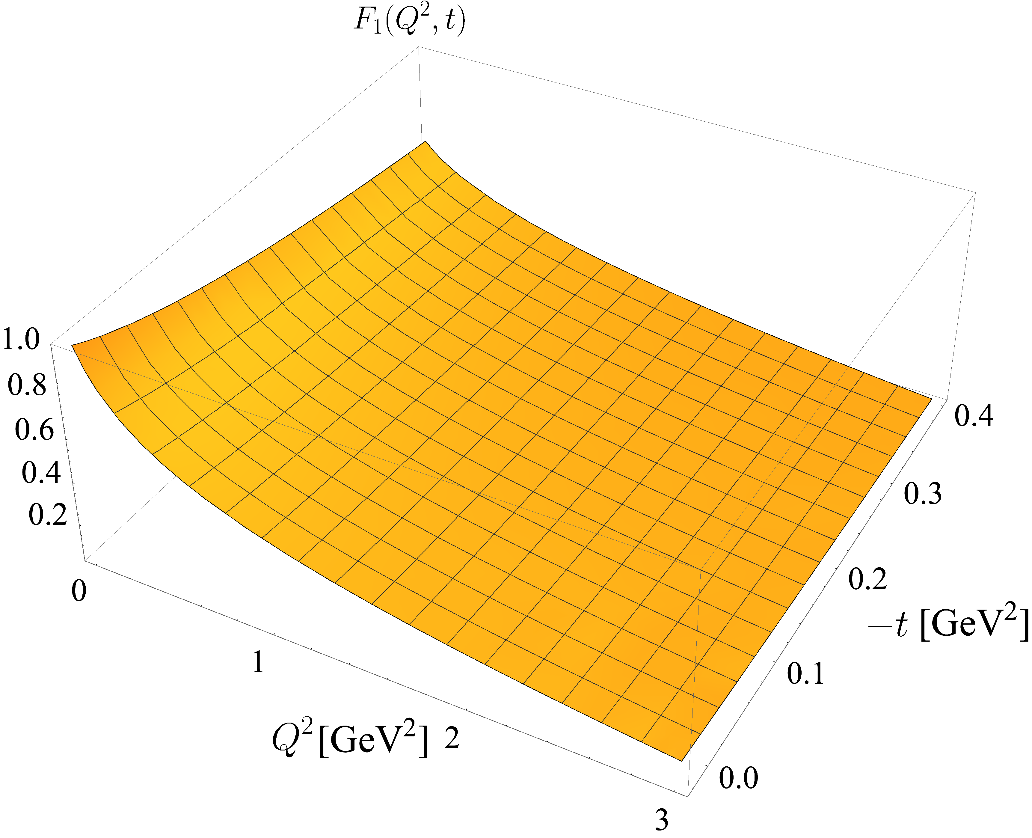
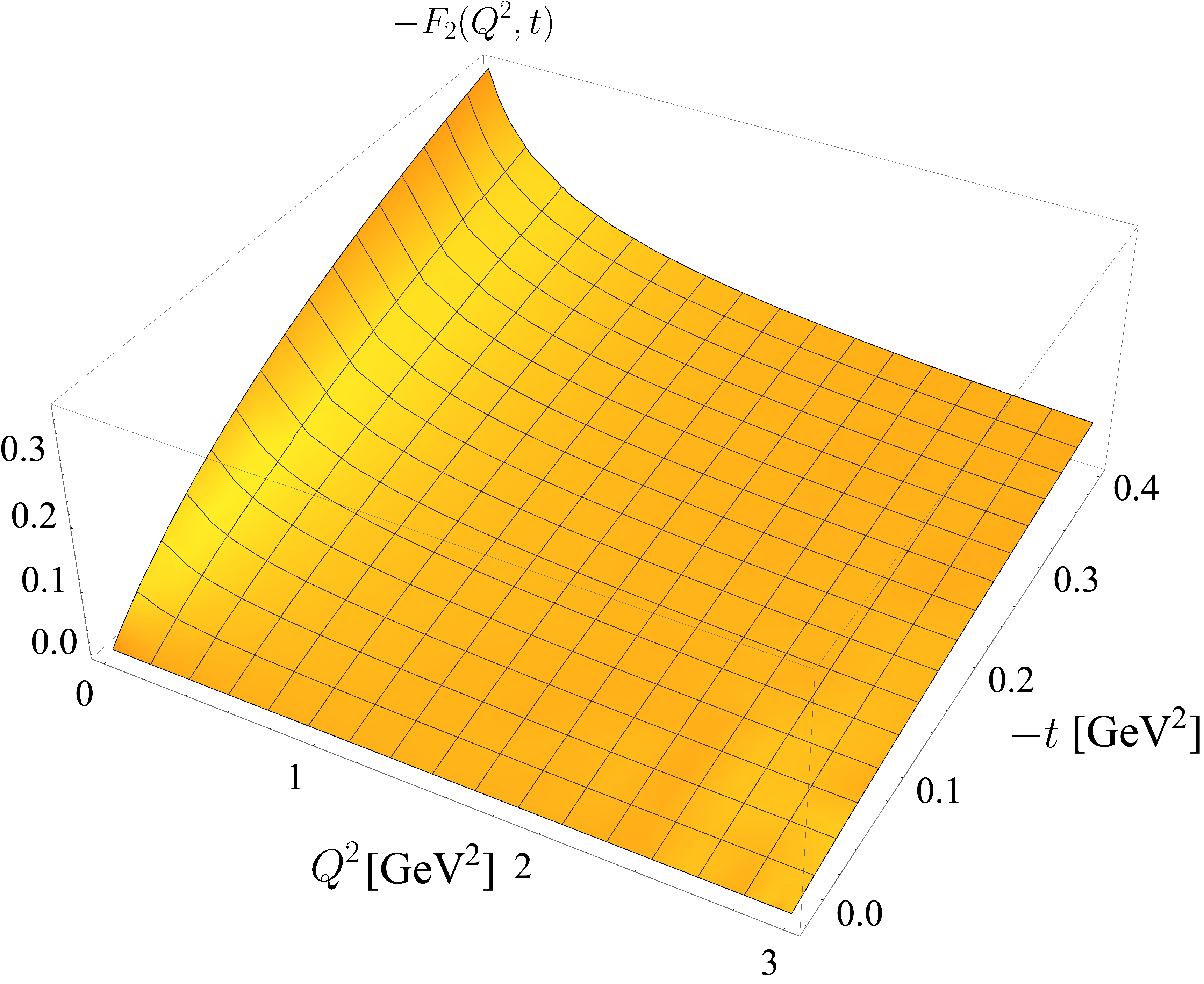
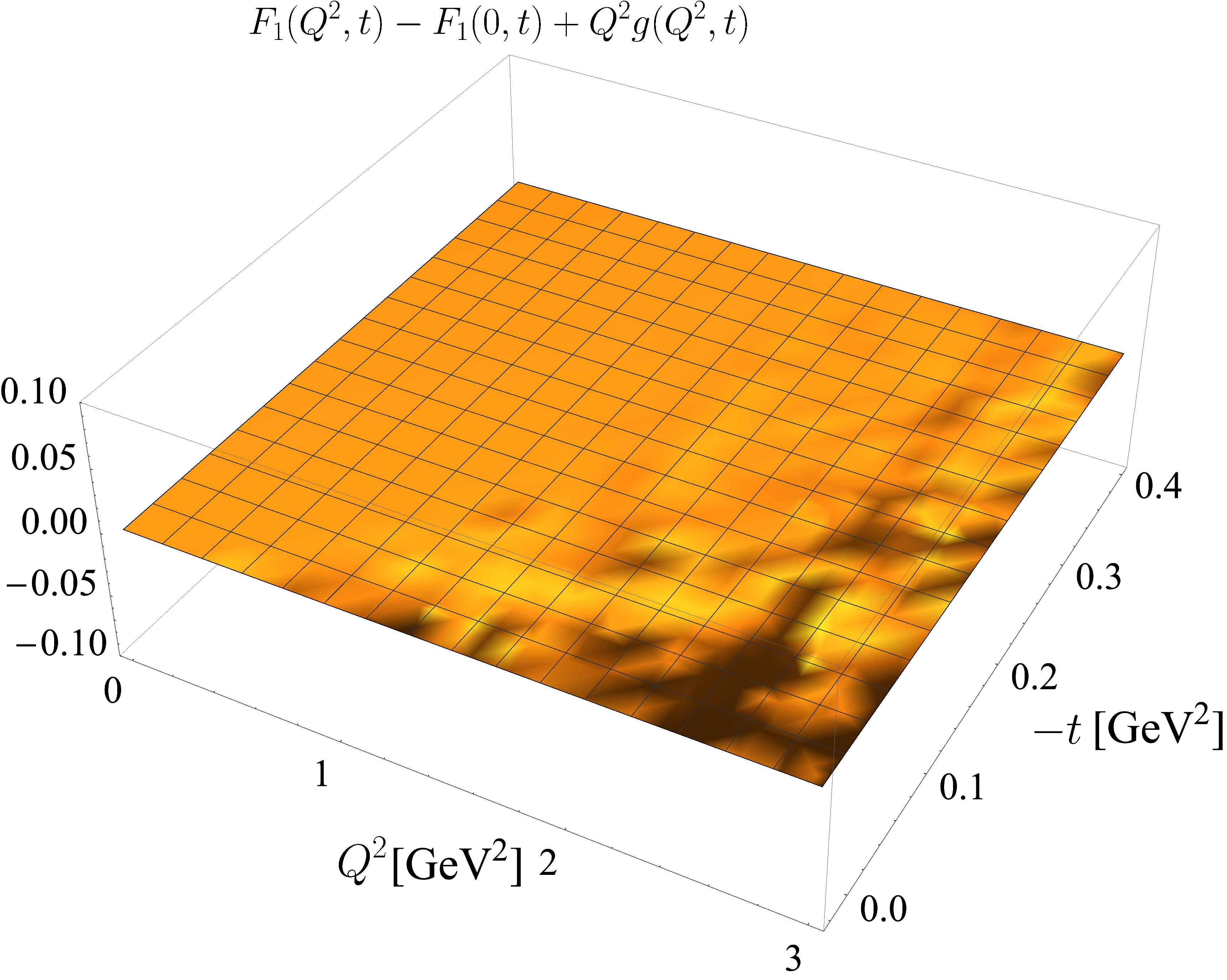
Figure 6: The 3D plots of $F_{1}(Q^{2},t)$ (top left), $F_{2}(Q^{2},t)$ (top right), $g(Q^{2},t)$ (bottom left) and the sum rule (bottom right) given by Eq. (11) for the spacelike momentum transfer region $0\leq Q^{2}\leq 3$ GeV² and $m^{2}_{\pi}\geq t\geq-0.4$ GeV². The used model parameters are $m_{q}=0.16$ GeV and $g_{\pi q{\bar{q}}}=1.11(2m_{q}/f^{\rm Exp}_{\pi})$.

The landscapes of the half-off-shell spacelike form factors given in Fig. 5 are shown in more detail in Fig. 6, as it is relevant for our forthcoming analysis of the experimental data. The figure represents the 3D plots of $F_{1}(Q^{2},t)$ (top left), $-F_{2}(Q^{2},t)$ (top right), $g(Q^{2},t)$ (bottom left) and the master equation (bottom right) given by Eq. (11) for the momentum transfer region $0\leq Q^{2}\leq 3$ GeV² and $m^{2}_{\pi}\geq t\geq-0.4$ GeV². While the form factor $F_{2}(Q^{2},t)$ goes to zero as $t\to m^{2}_{\pi}$, the form factor $g(Q^{2},t)$ is nonzero even in the on-mass-shell limit. Furthermore, $F_{1}(0,t)$ shows some dependencies on $t$, which is necessary to know in the case of extracting $F_{2}(Q^{2},t)$ from the pion electroproduction data. In particular, the value of $g(Q^{2}=0,t=m^{2}_{\pi})$ corresponds to the charge radius of a pion. The covariant and analytical model is checked against the fulfillment of the master equations, i.e. the sum rules given by Eqs. (11), (12), (15) and (16), and we display the fulfillment of Eq. (11) in the figure (bottom right) as an explicit illustration. The verification of these master equations gives not only an indirect check on the fulfillment of the WTI by the model, but also our numerical accuracy.

IV Extraction of the off-shell form factors from the experimental cross section

IV.1 Extraction of half-off-shell pion form factors

The off-shell form factor $F_{1}(Q^{2},t)$ can be extracted from the exclusive cross section for ${}^{1}{\rm H}(e,e^{\prime},\pi^{+})n$ in the kinematical region of small $t$, such that the $t$-channel process dominates near the pion pole at $t=m^{2}_{\pi}$ Blok2008 ; Huber2008 . To minimize background contributions, it is also necessary to separate out the longitudinal cross section $\sigma_{\rm L}$, via the Rosenbluth separation depending on the polarization states of the virtual photon in terms of the longitudinal differential cross section ($d\sigma_{\rm L}/dt$), the transverse differential cross section ($d\sigma_{\rm T}/dt$), and the two other differential cross sections due to interference  ($d\sigma_{\rm LT}/dt$ and $d\sigma_{\rm TT}/dt$).

Since the minimum physical value of $-t$ is nonzero and increases with the increasing value of $Q^{2}$ and decreasing value of the invariant mass $W$ of the produced pion-nucleon system, more reliable extraction of the on-shell pion form factor $F_{\pi}(Q^{2})=F_{1}(Q^{2},t=m^{2}_{\pi})$ should be performed at smaller $-t$ and higher $W$ (for a fixed $Q^{2}$) as discussed in Ref. Huber2008 . In Ref Huber2008 , ample discussions were devoted to the reliability issue of the Chew-Low extrapolation method and the use of the Regge model presented in Ref. VGL as well as the encouragement on additional models that one may use for the task of the form factor extraction.

The basis of the Chew-Low method is the Born-term model formula for the pion-pole contribution to $\sigma_{\rm L}$, where the pion-pole contribution to $\sigma_{\rm L}$ is given by

$$N\frac{d\sigma_{L}}{dt}=4\hbar c(eG_{\pi NN})^{2}\frac{-tQ^{2}}{(t-m^{2}_{\pi})^{2}}F^{2}_{\pi}(Q^{2})~{}.$$ (27)

Here, $e^{2}/(4\pi\hbar c)=1/137$ and the factor $N$ which depends on the flux factor used in the definition of $d\sigma_{\rm L}/dt$ is given by

$$N=32\pi\left(W^{2}-m^{2}_{p}\right)\sqrt{(W^{2}-m^{2}_{p})^{2}+Q^{4}+2Q^{2}(W^{2}+m^{2}_{p})}.$$ (28)

For the form factor $G_{\pi NN}(t)$, we follow the usual monopole type of parametrization

$$\ G_{\pi NN}(t) = G_{\pi NN}(m^{2}_{\pi})\left(\frac{\Lambda^{2}_{\pi}-m^{2}_{\pi}}{\Lambda^{2}_{\pi}~{}-~{}t}\right),$$ (29)

where $G_{\pi NN}(m^{2}_{\pi})=13.4$ and $\Lambda_{\pi}=0.80$ GeV have been taken in the extraction of $F_{\pi}$ from the Jefferson Lab experiment Huber2008 . We use the same values of $G_{\pi NN}(m^{2}_{\pi})$ and $\Lambda_{\pi}$ in our numerical extraction of the off-shell form factors $F_{1}(Q^{2},t)$ and $F_{2}(Q^{2},t)$ [or $g(Q^{2},t)$].

Table 1: Pion form factors extracted from experimental cross section for $d\sigma_{\rm L}/dt$ given in Table VII of Ref. Blok2008 vs solvable model with $m_{q}=0.14\pm 0.02$ GeV. The coupling constants, $g_{\pi q{\bar{q}}}=(1.32,1.20,1.11)(2m_{q}/f^{\rm Exp}_{\pi})$, are used for $m_{q}=(0.12,0.14,0.16)$ GeV, respectively. $(Q^{2},t)$ are in units of GeV², and $g(Q^{2},t)$ is in units of GeV^-2.

$Q^{2}$	$-t$	$F^{\rm Exp}_{1}(Q^{2},t)$	$F^{\rm Cov}_{1}(Q^{2},t)$	$F^{\rm Cov}_{1}(0,t)$	$g^{\rm Exp}(Q^{2},t)$	$g^{\rm Cov}(Q^{2},t)$
		$\langle Q^{2}\rangle=0.60$ GeV2,	$W=1.95$ GeV
0.526	0.026	0.502 $\pm$ 0.013	$0.487^{+0.032}_{-0.039}$	$0.891^{+0.019}_{-0.030}$	$0.740^{+0.060}_{-0.082}$	$0.768^{-0.024}_{+0.018}$
0.576	0.038	0.440 $\pm$ 0.010	$0.462^{+0.032}_{-0.039}$	$0.869^{+0.022}_{-0.033}$	$0.745^{+0.055}_{-0.075}$	$0.708^{-0.016}_{+0.008}$
0.612	0.050	0.413 $\pm$ 0.011	$0.443^{+0.030}_{-0.038}$	$0.849^{+0.024}_{-0.036}$	$0.712^{+0.058}_{-0.076}$	$0.664^{-0.010}_{+0.003}$
0.631	0.062	0.371 $\pm$ 0.014	$0.430^{+0.030}_{-0.036}$	$0.831^{+0.026}_{-0.038}$	$0.729^{+0.063}_{-0.082}$	$0.635^{-0.007}_{-0.002}$
0.646	0.074	0.340 $\pm$ 0.022	$0.419^{+0.030}_{-0.036}$	$0.814^{+0.027}_{-0.039}$	$0.734^{+0.076}_{-0.095}$	$0.611^{-0.004}_{-0.005}$
		$\langle Q^{2}\rangle=0.75$ GeV2,	$W=1.95$ GeV
0.660	0.037	0.397 $\pm$ 0.019	$0.435^{+0.030}_{-0.036}$	$0.870^{+0.023}_{-0.032}$	$0.717^{+0.063}_{-0.078}$	$0.660^{-0.012}_{+0.005}$
0.707	0.051	0.360 $\pm$ 0.017	$0.414^{+0.030}_{-0.035}$	$0.848^{+0.024}_{-0.036}$	$0.690^{+0.058}_{-0.075}$	$0.613^{-0.006}_{-0.001}$
0.753	0.065	0.358 $\pm$ 0.015	$0.394^{+0.029}_{-0.034}$	$0.827^{+0.026}_{-0.039}$	$0.623^{+0.054}_{-0.072}$	$0.574^{-0.003}_{-0.006}$
0.781	0.079	0.324 $\pm$ 0.018	$0.381^{+0.027}_{-0.033}$	$0.807^{+0.028}_{-0.040}$	$0.618^{+0.059}_{-0.074}$	$0.546^{-0.001}_{-0.009}$
0.794	0.093	0.325 $\pm$ 0.022	$0.371^{+0.028}_{-0.032}$	$0.789^{+0.029}_{-0.041}$	$0.584^{+0.065}_{-0.079}$	$0.526^{+0.003}_{-0.011}$
		$\langle Q^{2}\rangle=1.00$ GeV2,	$W=1.95$ GeV
0.877	0.060	0.342 $\pm$ 0.014	$0.366^{+0.027}_{-0.031}$	$0.834^{+0.026}_{-0.038}$	$0.561^{+0.046}_{-0.059}$	$0.533^{-0.001}_{-0.006}$
0.945	0.080	0.327 $\pm$ 0.012	$0.343^{+0.025}_{-0.030}$	$0.806^{+0.028}_{-0.040}$	$0.507^{+0.042}_{-0.055}$	$0.490^{+0.003}_{-0.010}$
1.010	0.100	0.311 $\pm$ 0.012	$0.322^{+0.024}_{-0.029}$	$0.781^{+0.030}_{-0.042}$	$0.465^{+0.042}_{-0.053}$	$0.454^{+0.006}_{-0.013}$
1.050	0.120	0.282 $\pm$ 0.016	$0.307^{+0.023}_{-0.027}$	$0.758^{+0.031}_{-0.043}$	$0.453^{+0.045}_{-0.056}$	$0.430^{+0.007}_{-0.015}$
1.067	0.140	0.233 $\pm$ 0.028	$0.297^{+0.023}_{-0.026}$	$0.737^{+0.032}_{-0.043}$	$0.472^{+0.057}_{-0.066}$	$0.412^{+0.009}_{-0.015}$
		$\langle Q^{2}\rangle=1.60$ GeV2,	$W=1.95$ GeV
1.455	0.135	0.258 $\pm$ 0.010	$0.237^{+0.018}_{-0.021}$	$0.742^{+0.032}_{-0.043}$	$0.332^{+0.029}_{-0.037}$	$0.347^{+0.010}_{-0.015}$
1.532	0.165	0.245 $\pm$ 0.010	$0.219^{+0.016}_{-0.020}$	$0.714^{+0.032}_{-0.044}$	$0.306^{+0.028}_{-0.035}$	$0.323^{+0.011}_{-0.016}$
1.610	0.195	0.222 $\pm$ 0.012	$0.201^{+0.015}_{-0.018}$	$0.688^{+0.033}_{-0.044}$	$0.289^{+0.028}_{-0.034}$	$0.302^{+0.012}_{-0.016}$
1.664	0.225	0.203 $\pm$ 0.013	$0.188^{+0.014}_{-0.017}$	$0.665^{+0.034}_{-0.045}$	$0.278^{+0.028}_{-0.035}$	$0.286^{+0.012}_{-0.016}$
1.702	0.255	0.227 $\pm$ 0.016	$0.177^{+0.014}_{-0.015}$	$0.644^{+0.034}_{-0.044}$	$0.245^{+0.029}_{-0.035}$	$0.274^{+0.012}_{-0.017}$
		$\langle Q^{2}\rangle=1.60$ GeV2,	$W=2.22$ GeV
1.416	0.079	0.270 $\pm$ 0.010	$0.259^{+0.019}_{-0.022}$	$0.807^{+0.028}_{-0.040}$	$0.379^{+0.027}_{-0.035}$	$0.387^{+0.006}_{-0.012}$
1.513	0.112	0.258 $\pm$ 0.010	$0.235^{+0.018}_{-0.021}$	$0.767^{+0.030}_{-0.043}$	$0.336^{+0.027}_{-0.035}$	$0.351^{+0.009}_{-0.014}$
1.593	0.139	0.251 $\pm$ 0.010	$0.217^{+0.016}_{-0.019}$	$0.738^{+0.032}_{-0.043}$	$0.306^{+0.026}_{-0.034}$	$0.327^{+0.010}_{-0.015}$
1.667	0.166	0.241 $\pm$ 0.012	$0.201^{+0.015}_{-0.018}$	$0.713^{+0.033}_{-0.044}$	$0.283^{+0.027}_{-0.033}$	$0.307^{+0.011}_{-0.016}$
1.763	0.215	0.200 $\pm$ 0.018	$0.179^{+0.013}_{-0.017}$	$0.672^{+0.034}_{-0.044}$	$0.268^{+0.029}_{-0.035}$	$0.280^{+0.011}_{-0.017}$
		$\langle Q^{2}\rangle=2.45$ GeV2,	$W=2.22$ GeV
2.215	0.145	0.188 $\pm$ 0.008	$0.146^{+0.010}_{-0.012}$	$0.732^{+0.033}_{-0.043}$	$0.246^{+0.018}_{-0.023}$	$0.265^{+0.010}_{-0.014}$
2.279	0.202	0.178 $\pm$ 0.008	$0.129^{+0.009}_{-0.011}$	$0.682^{+0.034}_{-0.044}$	$0.221^{+0.019}_{-0.023}$	$0.243^{+0.011}_{-0.015}$
2.411	0.245	0.163 $\pm$ 0.009	$0.109^{+0.008}_{-0.009}$	$0.650^{+0.037}_{-0.044}$	$0.202^{+0.019}_{-0.022}$	$0.224^{+0.011}_{-0.014}$
2.539	0.288	0.156 $\pm$ 0.011	$0.092^{+0.006}_{-0.007}$	$0.622^{+0.034}_{-0.043}$	$0.184^{+0.017}_{-0.022}$	$0.209^{+0.011}_{-0.014}$
2.703	0.365	0.150 $\pm$ 0.016	$0.068^{+0.004}_{-0.005}$	$0.579^{+0.033}_{-0.043}$	$0.159^{+0.018}_{-0.022}$	$0.189^{+0.011}_{-0.014}$

The experimental data for $d\sigma_{\rm L}/dt$ given in Table VII of Ref. Blok2008 are used for the extraction of the off-shell form factor $F^{\rm Exp}_{1}(Q^{2},t)$ using Eqs. (27)-(29), with the theory input from our model calculation presented in the previous section, Sec. III. Since there are no experimental data available for $F_{1}(Q^{2}=0,t)$, we extract $F^{\rm Exp}_{2}(Q^{2},t)$ [or $g^{\rm Exp}(Q^{2},t)$] from the WTI using the values of $F^{\rm Cov}_{1}(Q^{2}=0,t)$ obtained from the manifestly covariant model, i.e. $g^{\rm Exp}(Q^{2},t)=[F^{\rm Cov}_{1}(0,t)-F^{\rm Exp}_{1}(Q^{2},t)]/Q^{2}$. For the comparison of the covariant model with the experimental data, we use $m_{q}=(0.14\pm 0.02)$ GeV, checking the sensitivity of our covariant model calculation. The experimentally extracted off-shell form factors $F^{\rm Exp}_{1}(Q^{2},t)$ and $g^{\rm Exp}(Q^{2},t)$ and the corresponding results from the covariant model obtained from using $m_{q}=(0.14\pm 0.02)$ GeV are summarized in Table 1, in which $(Q^{2},-t)$ values are classified into six different sets in terms of average $\langle Q^{2}\rangle$ and the invariant mass $W$ following Ref. Blok2008 . To check the consistency of our experimental extraction of the form factors, we computed the master equation using the values of $F^{\rm Exp}_{1}(Q^{2},t)$, $F^{\rm Cov}_{1}(0,t)$ and $g^{\rm Exp}(Q^{2},t)$ given in Table 1. The attained 3D plot of the master equation Eq. (11) is shown in Fig. 7. As we have already used Eq. (11) to obtain $g^{\rm Exp}(Q^{2},t)$, this may be regarded as an obvious cross-check just for the purpose of illustration.

Figure 7: The 3D plot of the master equation (11) built with our experimental extraction of the off-shell pion form factors. In computing Eq. (11), we use the values of $F^{\rm Exp}_{1}(Q^{2},t)$, $F^{\rm Cov}_{1}(0,t)$, and $g^{\rm Exp}(Q^{2},t)$ given in Table 1.

Figure 8: The extracted off-shell pion form factors: $F^{\rm Exp}_{1}(Q^{2},t)$ (top) and $g^{\rm Exp}(Q^{2},t)$ (bottom) given in Table 1.

In Table 1, we note that the $Q^{2}$ and/or $-t$ evolution of the extracted values of $F^{\rm Exp}_{1}(Q^{2},t)$ is somewhat different from the result of $F_{1}(Q^{2},t)$ due to our covariant analytic model calculation. This difference may not be a surprise though, not only due to the simplicity of the covariant analytic model but also due to the limitation of the Chew-Low extrapolation involving the pion-nucleon form factor in crossing the disallowed kinematic region $t>0$ of the electroproduction process. While the improvement of the model deserves interest with respect to the QCD dynamics of the pion, it suggests the direct extraction of the off-shell pion form factors in lieu of the extrapolation procedure involving the disallowed kinematic region from the differential cross section of the electroproduction data.

The extracted off-shell form factors $F^{\rm Exp}_{1}(Q^{2},t)$ and $g^{\rm Exp}(Q^{2},t)$ from the 30 data points in Table 1 are plotted in Fig. 8 with respect to $Q^{2}$ and $t$. The overall momentum dependences of $Q^{2}$ and $t$ resemble the results of the covariant analytic model as shown in Fig. 6. While the data seem to exhibit the stronger variation with respect to $Q^{2}$ and $t$ than the model result as also noted in Table 1, the main features captured in the variation appear consistent between Figs. 6 and 8 from the model calculation and the data extraction, respectively.

IV.2 Comparison of extracted vs model form factors

The on-shell pion form factors $F_{1}(Q^{2},m^{2}_{\pi})$ (black lines) and $g(Q^{2},m^{2}_{\pi})$ (blue lines) from the covariant model for the spacelike region $Q^{2}>0$ are shown in Fig. 9 and compared with the extracted values of $F^{\rm Exp}_{1}(Q^{2},t=m^{2}_{\pi})$ (black data) and $g^{\rm Exp}(Q^{2},t=m^{2}_{\pi})=[1-F^{\rm Exp}_{1}(Q^{2},t=m^{2}_{\pi})]/Q^{2}$ (blue data). The model parameters in Fig. 9 are $m_{q}=(0.12,0.16)$ GeV using the variation of the couplings $g_{\pi q{\bar{q}}}=(1.32\pm 0.04,1.11\pm 0.04)(2m_{q}/f^{\rm Exp}_{\pi})$, respectively. The solid and dashed lines represent the results obtained from $m_{q}=0.12$ and 0.16 GeV using the upper and lower limits of the corresponding $g_{\pi q{\bar{q}}}$. We should note that while the upper (lower) line of $F_{1}(Q^{2},m^{2}_{\pi})$ corresponds to the lower (upper) limit of $g_{\pi q{\bar{q}}}$, the upper (lower) line of $g(Q^{2},m^{2}_{\pi})$ corresponds to the upper (lower) limit of $g_{\pi q{\bar{q}}}$. Unlike the form factor $F_{2}(Q^{2},t)$, the form factor $g(Q^{2},t)$ does not vanish in the on-shell limit. We note that the current Particle Data Group PDG2018 average $r^{\rm Exp}_{\pi}=\sqrt{\langle r^{2}_{\pi}\rangle}=(0.672\pm 0.008)$ fm for the rms value of the pion charge radius corresponds to $g^{\rm Exp}(Q^{2}=0,m^{2}_{\pi})=(1.953\pm 0.023)$ GeV^-2. Although the more realistic model than the present one may be required to predict $g(Q^{2},m^{2}_{\pi})$ more accurately, we note that the form factor $g(Q^{2},m^{2}_{\pi})$ should be regarded as the physical observable in the on-mass-shell limit on par with the charge form factor $F_{1}(Q^{2},m^{2}_{\pi})$. In this respect, it is interesting to observe that $g^{\rm Exp}(Q^{2},t=m^{2}_{\pi})=[1-F^{\rm Exp}_{1}(Q^{2},t=m^{2}_{\pi})]/Q^{2}$ exhibits a rather large fluctuation near $Q^{2}=0$, which may reflect a correspondingly large uncertainty in determining the pion charge radius.

Figure 9: The on-shell pion form factors $F_{1}(Q^{2},m^{2}_{\pi})$ (black lines) and $g(Q^{2},m^{2}_{\pi})$ (blue lines) for the spacelike momentum transfer region $0\leq Q^{2}\leq 2$ GeV² compared with the experimental data for $F^{\rm Exp}_{1}$ (black data) and $g^{\rm Exp}$ (blue data). The used model parameters are $m_{q}=(0.12,0.16)$ GeV using the variation of the couplings $g_{\pi q{\bar{q}}}=(1.32\pm 0.04,1.11\pm 0.04)(2m_{q}/f^{\rm Exp}_{\pi})$, respectively, and we show only the upper and lower limits of $g_{\pi q{\bar{q}}}$.

Figure 10: The comparison of the off-shell pion form factors $F_{1}(Q^{2},t)$ and $g(Q^{2},t)$ given in Table 1 and those obtained from the covariant model. The top and bottom panels show $Q^{2}-$ and $t$ dependences of $F_{1}(Q^{2},t)$ (left) and $g(Q^{2},t)$ (right), respectively.

The extracted off-shell pion form factors $F_{1}(Q^{2},t)$ and $g(Q^{2},t)$ given in Table 1 and those obtained from the covariant model are compared in Fig. 10. The top panel shows the $Q^{2}$ dependence of $F_{1}(Q^{2},t)$ (left) and $g(Q^{2},t)$ (right) collecting all the data in Table 1 regardless of $t$ values, while bottom panel shows the $t$ dependences of $F_{1}(Q^{2},t)$ (left) and $g(Q^{2},t)$ (right) collecting all the data in Table 1 regardless of $Q^{2}$ values. The black and blue data represent, respectively, the extracted data from the JLab experiment Blok2008 and the results of the covariant model obtained from Eqs. (III.1) and (20) using the quark mass $m_{u(d)}=0.14\pm 0.02$ GeV. A rather significant difference in the slope of $Q^{2}$ evolution between $F^{\rm Exp}_{1}(Q^{2},t)$ and $F^{\rm Cov}_{1}(Q^{2},t)$ in the top left panel of Fig. 10 may be understood from the QCD effect on $F^{\rm Exp}_{1}(Q^{2},t)$ from the gluon exchange between the quark and antiquark that gets important as $Q^{2}$ gets larger, while the solvable model result $F^{\rm Cov}_{1}(Q^{2},t)$ does not accommodate this perturbative QCD feature. It is interesting to see, however, that the newly introduced form factor $g(Q^{2},t)$ defined by Eq.(10) appears independent of this feature. The model-independent experimental extraction of $F_{1}(0,t)$ appears indispensable to make the more accurate assessment on the $g(Q^{2},t)$ behavior without involving any model dependence.

V Conclusions

In this work, we investigated the pion electromagnetic half-off-shell form factors $F_{1}(Q^{2},t)$ and $F_{2}(Q^{2},t)$ using the manifestly covariant fermion field theory model.

In this simple covariant model, since our result for $F_{1}(Q^{2},t=m^{2}_{\pi})$ includes a UV divergence $1/\epsilon$ term of the dimensional regularization, we fixed the normalization of the electric charge via the subtractive renormalization, i.e. $F^{\rm ren}_{1}(Q^{2},t)=1+[F_{1}(Q^{2},t)-F_{1}(0,m^{2}_{\pi})]$, as the loop correction to the charge form factor must vanish at $Q^{2}=0$. We used $F^{\rm ren}_{1}(Q^{2},t)$ as our off-shell form factor $F_{1}(Q^{2},t)$ throughout the analysis. Our result for $F_{2}(Q^{2},t)$ is, however, free from the UV divergence. In our covariant model with the constituent quark mass $m_{q}$ as a free parameter, we note that the $\pi q{\bar{q}}$ coupling constant $g_{\pi q{\bar{q}}}$ is related with the pion decay constant $f_{\pi}$ together with the constiuent quark mass via $g_{\pi q{\bar{q}}}\approx 2m_{q}/f_{\pi}$. In our numerical calculation, however, we used $g_{\pi q{\bar{q}}}$ as a free parameter to find the best fit for the form factors compared to the experimental data. It turns out that our best fits for the constituent quark mass ranges $0.12\leq m_{q}\leq 0.16$ GeV and the corresponding coupling $g_{\pi q{\bar{q}}}$ are consistent with the values of $2m_{q}/f_{\pi}$ within 15$\%$ errors.

We also note that the ratio of $F_{2}(Q^{2},t)$ to $t-m^{2}_{\pi}$ is nonzero in the limit of $t\to m^{2}_{\pi}$ while $F_{2}(Q^{2},t)$ goes to zero as $t\to m^{2}_{\pi}$. This led us to define the new form factor $g(Q^{2},t)=F_{2}(Q^{2},t)/(t-m^{2}_{\pi})$, which should be measurable even in the on-mass-shell limit on par with the usual charge form factor $F_{1}(Q^{2},m^{2}_{\pi})$. In particular, we obtain the sum rule given by Eq. (11) which relates $g(Q^{2},t)$ to $F_{1}(Q^{2},t)$ and note that the value of $g(Q^{2}=0,t=m^{2}_{\pi})$ corresponds to the charge radius of a pion.

According to Eq. (11), however, one needs the information of $F_{1}(0,t)$ to determine $g(Q^{2},t)$, while no data of $F_{1}(Q^{2},t)$ exist at $Q^{2}=0$ for $t<0$. In this work, we used a simple covariant model to provide at least a clear example of demonstration for the simultaneous extraction of both $F_{1}(Q^{2},t)$ and $g(Q^{2},t)$ (or $F_{2}(Q^{2},t)$). In our numerical calculations, we show the 3D plots of $F_{1(2)}(Q^{2},t)$ and $g(Q^{2},t)$ in terms of $(Q^{2},t)$ values as shown in Figs. 5 and 6.

Our extracted values of the pion form factors obtained from the experimental cross section for $d\sigma_{\rm L}/dt$ given in Table VII of Ref. Blok2008 and the results obtained from the solvable model with $m_{q}=0.14\pm 0.02$ GeV are summarized in Table 1. The extracted off-shell form factors $F^{\rm Exp}_{1}(Q^{2},t)$ and $g^{\rm Exp}(Q^{2},t)$ from the 30 data points in Table 1 are plotted in Fig. 8 with respect to $Q^{2}$ and $t$. The main features captured in the variation appear consistent between Figs. 6 and 8 from the model calculation and the data extraction, respectively.

However, the comparison of the extracted values of the form factors with covariant model results indicates that the evolution in $Q^{2}$ and/or $t$ are not in full agreement between the extracted vs. model form factors. On the one hand, this is not unexpected as the internal QCD dynamics of the pion probed by the electroproduction data should not be restricted only to its valence content, while the present model for the pion coupling to the quark and antiquark is just of a pointlike form. A rather significant difference in the slope of $Q^{2}$ evolution between $F^{\rm Exp}_{1}(Q^{2},t)$ and $F^{\rm Cov}_{1}(Q^{2},t)$ in the top left panel of Fig. 10 may be an indication of lacking the QCD effect from the gluon exchange between quark and antiquark that gets important as $Q^{2}$ gets larger. The QCD nonperturbative dynamics for the self-energies of quarks and gluons, and the vertices of pion-quark, photon-quark, etc., deserves further study exploring the 3D imaging of the off-shell form factors. On the other hand, the analysis of the electroproduction data by the Chew-Low method demands the pion-nucleon form factor as input, which indeed is a simplification and works only close to the pion pole. Such a limitation may be also reflected in our extraction of the form factors from the data, which in part corroborates the difference between the extracted vs model form factors.

Nevertheless, the overall representation of the trends of the extracted form factors in the $(Q^{2},t)$ plane by the present constituent model indicates that our analysis goes beyond its obvious limitations. It encourages more in-depth theoretical and experimental efforts to reveal the 3D imaging of the off-shell pion form factors.

Appendix A Explicit Calculation of Eqs. (III.1) and  (20)

Using the Feynman parametrization for the three propagators, we obtain

$$\frac{1}{N_{k}N_{k+q}N_{p-k}}=\int^{1}_{0}\;dx\int^{x}_{0}\;dy\frac{2!}{[(k+E)^{2}-C]^{3}},$$ (30)

where $E=(x-y)q-yp$, $C=(x-y)(x-y-1)q^{2}-y(1-y)t-2y(x-y)q\cdot p+m^{2}_{q}$, and $q\cdot p=(m^{2}_{\pi}+Q^{2}-t)/2$.

After combining Eqs. (17),  (18), and (30) and shifting the 4-momentum variable of integration as $k^{\prime}=k+E$, we obtain the trace term as

$$S^{\mu}=-4(C^{\mu}_{1}k^{\prime 2}+C^{\mu}_{2}),$$ (31)

where

$$C^{\mu}_{1} = \frac{1}{2}[(1+3y)p^{\mu}+(2+3y-3x)q^{\mu}],$$

$$C^{\mu}_{2} = p^{\mu}[(1+y)(E^{2}-m^{2}_{q})-E\cdot q+2yE\cdot q-yq\cdot p]$$ (32)

$$+ q^{\mu}[(1-x+y)(E^{2}-m^{2}_{q})+(1-2x+2y)E\cdot p$$

$$\hskip 99.58464pt+\;(x-y)q\cdot p].$$

Using the dimensional regularization in $d(=4-2\epsilon)$ dimensions, we obtain the two form factors $F_{1}(Q^{2},t)$ and $F_{2}(Q^{2},t)$ from the definition of $\Gamma^{\mu}=(p^{\prime}+p)^{\mu}F_{1}(Q^{2},t)+q^{\mu}F_{2}(Q^{2},t)$ as given by Eqs.(III.1) and (20), respectively.

References

• (1) E. B. Dally, D. J. Drickey, J. M. Hauptman, C. F. May, D. H. Stork, J. A. Poirier et al., Phys. Rev. D 24, 1718 (1981).
• (2) E. B. Dally, J. M. Hauptman, J. Kubic, D. H. Stork, A. B. Watson, Z. Guzik et al., Phys. Rev. Lett. 48, 375 (1982).
• (3) S. R. Amendolia et al., Nucl. Phys. B277, 168 (1986).
• (4) S. R. Amendolia et al., Phys. Lett. B 146, 116 (1984).
• (5) M. Carmignotto, Ph.D. Dissertation, The Catholic University of America, 2017.
• (6) J. D. Sullivan, Phys. Rev. D 5, 1732 (1972).
• (7) H. P. Blok et al., Phys. Rev. C 78, 045202 (2008).
• (8) G. M. Huber et al.,Phys. Rev. C 78, 045203 (2008).
• (9) T. Horn et al., Phys. Rev. C 78, 058201 (2008).
• (10) T. Horn et al., Phys. Rev. Lett. 97, 192001 (2006); J. Volmer et al., Phys. Rev. Lett. 86, 1713 (2001); V. Tadevosyan et al., Phys. Rev. C 75, 055205 (2007).
• (11) T. Horn and C. D. Roberts, J. Phys. G 43, 073001 (2016).
• (12) T. E. Rudy, H. W. Fearing, and S. Scherer, Phys. Rev. C 50, 447 (1994).
• (13) C. Weiss, Phys. Lett. B 333, 7 (1994).
• (14) S.-X. Qin, C. Chen, C. Mezrag, and C. D. Roberts, Phys. Rev. C 97, 015203 (2018).
• (15) F. Gao, L. Chang, Y.-X. Liu, C. D. Roberts, and P. C. Tandy, Phys. Rev. D 96, 034024 (2017).
• (16) A. M. Bincer, Phys. Rev. 118, 855 (1960).
• (17) H. W. L. Naus and J. H. Koch, Phys. Rev. C 36, 2459 (1987).
• (18) P. C. Tiemeijer and J. A. Tjon, Phys. Rev. C 42, 599 (1990).
• (19) J. C. Ward, Phys. Rev. 78, 182 (1950).
• (20) Y. Takahashi, Nuovo Cimento 6, 371 (1957).
• (21) X. Song, J. P. Chen, and J. S. McCarthy, Z. Phys. A 341, 275 (1992).
• (22) J. W. Bos and J. H. Koch, Nucl. Phys. A563, 539 (1993).
• (23) K. Nishijima, Phys. Rev. 122, 298 (1961).
• (24) G. Barton, Introduction to Dispersion Techniques in Field Theory (Benjamin, New York, 1965).
• (25) H. W. L. Naus, J. P. B. C. de Melo and T. Frederico, Few-Body Syst.  24, 99 (1998).
• (26) T. K. Pedlar et al., Phys. Rev. Lett. 95, 261803 (2005).
• (27) K. K. Seth, S. Dobbs, Z. Metreveli, A. Tomaradze, T. Xiao, and G. Bonvicini, Phys. Rev. Lett. 110, 022002 (2013).
• (28) M. Vanderhaeghen, M. Guidal, and J. M. Laget, Phys. Rev. C 57, 1454 (1998).
• (29) M. Tanabashi et al. (Particle Data Group), Phys. Rev. D 98, 030001 (2018).